1. Introduction
Shock reflection is a fundamental phenomenon in supersonic flows. It occurs when an incident shock interacts with a wall or a symmetric surface, and is frequently found in supersonic inlets. The pressure, temperature and density increase sharply behind the shock, which can significantly damage inlet performance and even alter the overall aerodynamic characteristics of the vehicle (Huang et al. Reference Huang2023).
Shock reflection is generally divided into two types: regular reflection and Mach reflection. Schematic illustrations of regular reflection and Mach reflection are shown in figures 1(a) and 1(b), respectively. For regular reflection, the incident shock (
 $i$
) is reflected as a reflected shock (
 $r$
). For Mach reflection, the incident shock (
 $i$
) generates a reflected shock (
 $r$
), a Mach stem (
 $m$
) and a slipline (
 $s$
), and these three structures are connected to a triple point (
 $T$
).
After von Neumann (Reference von Neumann1943, Reference von Neumann1945) established the method to obtain the flow parameters in the vicinity of a reflecting point or triple point for shock reflection, and developed the transition criteria between regular reflection and Mach reflection, scholars have conducted extensive research on shock reflection problems. These studies include the double solution and hysteresis loop phenomena (Henderson & Lozzi Reference Henderson and Lozzi1979; Hornung, Oertel & Sandeman Reference Hornung, Oertel and Sandeman1979; Teshukov Reference Teshukov1989; Chpoun et al. Reference Chpoun, Passerel, Li and Ben-Dor1995; Vuillon, Zeitoun & Ben-Dor Reference Vuillon, Zeitoun and Ben-Dor1995; Ivanov et al. Reference Ivanov, Ben-Dor, Elperin, Kudryavtsev and Khotyanovsky2001; Ben-Dor et al. Reference Ben-Dor, Ivanov, Vasilev and Elperin2002; Hornung Reference Hornung2014), strong Mach reflection (Qin et al. Reference Qin, Shi, Dowell, Pei and Huang2022), curved shock reflection (Shi et al. Reference Shi, You, Zheng and Zhu2023; Zhang et al. Reference Zhang, Xu, Shi, Zhu and You2023; Yan et al. Reference Yan, Han, Shi and You2024), multiple incident shock reflections (Guan, Bai & Wu Reference Guan, Bai and Wu2018; Guan, Bai & Wu Reference Guan, Bai and Wu2020; Bai Reference Bai2024; Li & Bai Reference Li and Bai2025), and shock reflection with incident shock–expansion wave interaction (Yao, Li & Wu Reference Yao, Li and Wu2013; Bai Reference Bai2023; Baby, Paramanantham & Rajesh Reference Baby, Paramanantham and Rajesh2024; He & Shi Reference He and Shi2025), as well as shock reflection in axisymmetric flow (Shoesmith & Timofeev Reference Shoesmith and Timofeev2021; Shi et al. Reference Shi, You, Zheng and Zhu2023; Shoesmith & Timofeev Reference Shoesmith and Timofeev2025).
Among many aspects, the size issue of a Mach reflection flow field structure has attracted much attention, because Mach reflection has higher stagnation pressure loss than regular reflection, and excessively high Mach stem height in a duct may act to ‘unstart’ the flow, resulting in a subsonic region (Azevedo & Liu Reference Azevedo and Liu1993). Hornung & Robinson (Reference Hornung and Robinson1982) pointed out that the Mach stem height is affected by the pressure decreasing information from the trailing edge expansion fan. This pressure information will be carried out to the subsonic flow region below the slipline, then transported upstream to the triple point through the subsonic region. They postulated a functional form for Mach stem height as
 \begin{equation} \frac {H_{T}}{w}=f\! \left ( M_{0},\theta _{w},\gamma ,\frac {H_{\!R}}{w}\right )\!, \end{equation}
which means that the Mach stem height
 $H_{T}$
depends on the inflow Mach number
 $ M_{0}$
, the wedge angle
 $\theta _{w}$
, the ratio of specific heats of gas
 $ \gamma$
, and the trailing edge height
 $H_{\!R}$
.
Since then, numerous studies on modelling conventional Mach reflection have been conducted (Li & Ben-Dor Reference Li and Ben-Dor1997; Mouton & Hornung Reference Mouton and Hornung2007; Gao & Wu Reference Gao and Wu2010; Bai & Wu Reference Bai and Wu2017, Reference Bai and Wu2021; Chernyshov, Savelova & Kapralova Reference Chernyshov, Savelova and Kapralova2021; Choe Reference Choe2022).
Schematic illustrations of shock reflections: (a) regular reflection, and (b) conventional Mach reflection.

In the models of Azevedo & Liu (Reference Azevedo and Liu1989,Reference Azevedo and Liu1993), two main assumptions are made. The slipline, the leading characteristic line, the Mach stem and the reflected shock are all assumed to be straight lines. In addition, the transmitted leading characteristic line of the trailing edge expansion fan is assumed to intersect the slipline at the sonic throat. The model correctly captures the qualitative trend of Mach stem height variation with respect to other factors, but the quantitative discrepancy between the experiments and model predictions is substantial.
Li & Ben-Dor (Reference Li and Ben-Dor1997) improved these two assumptions. In their model, the Mach stem, reflected shock and slipline are assumed as curved lines rather than straight lines. The sonic throat is located downstream of the transmitted leading characteristic line. An additional assumption introduced in their model is that the flow deflection angle and the pressure remain constant along the characteristic lines. Mouton & Hornung (Reference Mouton and Hornung2007) relax several assumptions in the work of Azevedo & Liu (Reference Azevedo and Liu1993) and propose a model capable of predicting both the Mach stem height and its growth rate.
Gao & Wu (Reference Gao and Wu2010) considered the influence of the Mach waves (secondary waves) above the free part of the slipline. To match the pressure decrease in the quasi-one-dimensional duct below the slipline, the secondary waves were generated over the slipline. Based on this observation, they proposed a discrete model involving the secondary waves, which produced more accurate results than previous models, and highlighted the importance of these waves. Building on this development, Bai & Wu (Reference Bai and Wu2017) derived an analytical model that provided explicit expressions for both the shape of the slipline and the reflected shock wave. In their formulation, the transmitted characteristic lines were still assumed to be straight.
Based on the earlier models, several new models have been proposed, improving the details of flow structures. For instance, Chernyshov et al. (Reference Chernyshov, Savelova and Kapralova2021) developed a quick analytical model for shock reflection. Bai & Wu (Reference Bai and Wu2021) and Choe (Reference Choe2022) proposed models that provide explicit expressions by employing geometrical relations.
According to these theoretical models, it has been found that the Mach stem height decreases with increasing inflow Mach number or wedge trailing edge height, and increases with increasing wedge angle (Gao & Wu Reference Gao and Wu2010; Bai & Wu Reference Bai and Wu2021). In particular, numerical simulations further indicate that the relationship between Mach stem height and wedge trailing edge height is approximately linear. This linear behaviour is also exhibited in several theoretical models (Schotz et al. Reference Schotz, Levy, Ben-Dor and Igra1997; Bai & Wu Reference Bai and Wu2021; Qin et al. Reference Qin, Shi, Dowell, Pei and Huang2022).
In summary, theoretical models of Mach reflection have attracted great attention and have been studied extensively for many decades. Most of these models divide the flow field into several regions, including the interaction between the reflected shock and the trailing edge expansion fan, the slipline region, and the transmitted Mach wave region. The solutions for these different flow field regions rely on different assumptions and processing methods, which in turn influence the calculation accuracy of the models. However, there has been no systematic investigation into the sensitivity of these methods for each flow field region. In addition, although existing theoretical models are able to capture the general variation law of the Mach stem height, they still have deficiencies in slope prediction accuracy.
Therefore, this paper will focus on the influence of sub-models in Mach reflection theory and on deriving an accurate predictive formula for the Mach stem height. The rest of this paper is organised as follows. Section 2 presents an updated analytical shock reflection model, building upon the work of Bai (Reference Bai2023). Section 3 investigates the sensitivity of various sub-models in Mach reflection, and evaluates the validity of the underlying assumptions. Section 4 examines the relationship between Mach stem height and trailing edge height over an extended range, and proposes predictive formulas for both slope and intercept. Finally, § 5 concludes the paper with a summary and further remarks.
Schematic of Mach reflection.

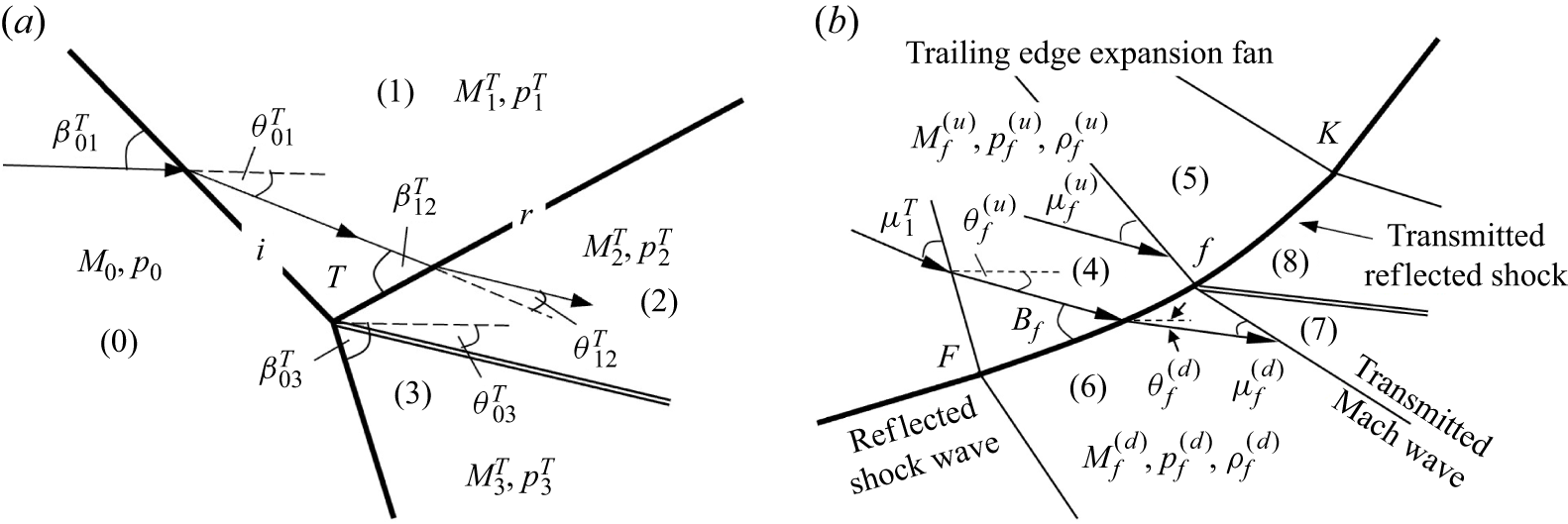
Definition of flow parameters (a) near the triple point and (b) near the interactive part of the reflected shock.

2. An updated model for Mach stem height
Bai (Reference Bai2023) provided a Mach stem height model accounting for the interaction between the incident shock and the trailing edge expansion fan, an occasion for wedge trailing edge height
 $H_{\!R}$
greater than the maximum
 $H_{R,\textit{max}}$
as established by Li & Ben-Dor (Reference Li and Ben-Dor1997). The updated Mach stem height model here is a model updated from the model of Bai (Reference Bai2023) by not considering the incident shock/trailing edge expansion fan, i.e. for
 $H_{\!R}\lt H_{R,\textit{max}}$
. Compared to the model of Bai & Wu (Reference Bai and Wu2017), this model uses a compatibility relation along the characteristic line approaching the slipline from above this slipline.
2.1. Updated Mach stem height model
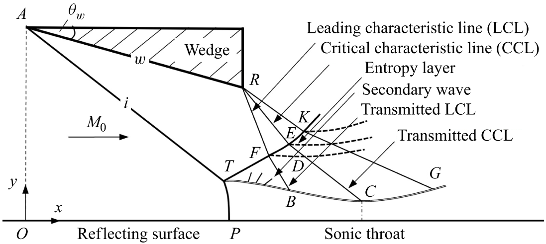
Figure 2 is a schematic of Mach reflection, which shows that the flow field mainly includes four structures: the reflected shock (
 $\textit{TK}$
), the transmitted Mach waves (
 $\textit{BGKF}$
), the free part of the slipline (
 $\textit{TB}$
), and the interactive part of the slipline (
 $\textit{BG}$
).
The flow parameters in the vicinity of the triple point (
 $T$
) are associated with the triple-shock theory (von Neumann Reference von Neumann1943). Specifically, as shown in figure 3(a), these parameters include the shock angles (
 $\beta _{01}^{T}$
,
 $\beta _{12}^{T}$
and
 $\beta _{03}^{T}$
), the flow deflection angles (
 $\theta _{01}^{T}$
,
 $\theta _{12}^{T}$
and
 $\theta _{03}^{T}$
), pressure (
 $p_{1}^{T}$
,
 $p_{2}^{T}$
and
 $p_{3}^{T}$
) and Mach numbers (
 $M_{1}^{T}$
,
 $M_{2}^{T}$
and
 $M_{3}^{T}$
). The Mach angle
 $\mu$
is given by
 $\mu =\arcsin ({1}/{M})$
.
2.1.1. The reflected shock sub-model
As shown in figure 2, the reflected shock is divided into two parts (
 $\textit{TF}$
and
 $\textit{FK}$
) depending on whether it interacts with the trailing edge expansion fan. The intersection of the reflected shock with the first characteristic line is point
 $F$
. The intersection of the reflected shock with the last characteristic line is point
 $K$
. The flow parameters near the reflected shock are illustrated in figure 3(b). Superscripts
 $(u)$
and
 $(d)$
denote the upstream and downstream flow parameters of the reflected shock, respectively.
For
 $\textit{TF}$
, the reflected shock is straight and the shock intensity is constant. Based on geometrical relations, the coordinates of point
 $F$
are given by
 \begin{equation} \left \{ \begin{array}{l} x_{F}=\dfrac {H_{\!R}-y_{T}+x_{T}\tan \left ( \beta _{12}^{T}-\theta _{w}\right ) +x_{R}\tan \left ( \mu _{1}^{T}+\theta _{w}\right ) }{\tan \left ( \beta _{12}^{T}-\theta _{w}\right ) +\tan \left ( \mu _{1}^{T}+\theta _{w}\right ) }, \\[15pt] y_{F}=y_{T}+\left ( x_{F}-x_{T}\right ) \tan \left ( \beta _{12}^{T}-\theta _{w}\right )\!. \end{array} \right . \end{equation}
For
 $\textit{FK}$
, due to its interaction with the expansion wave, the reflected shock is curved. Consider a typical point
 $f$
on
 $\textit{FK}$
as shown in figure 3(b).
-
(i) The flow parameters in region (5) are related to those in region (4) by the Prandtl–Meyer relation (B4) and isentropic relations (B5).
-
(ii) The flow parameters in region (6) are related to those in region (4) by shock relations (B1)–(B3).
-
(iii) The flow parameters in region (7) are related to those in region (4) by the Prandtl–Meyer relation (B4) and the isentropic relation (B5), and the flow parameters in region (8) are related to those in region (5) by shock relations (B1)–(B3).
-
(iv) The pressures and flow angles in region (7) and region (5) are equal.
Based on these relations, the shock angle
 $\beta _{\!f}$
and the downstream flow parameters (the flow deflection angle
 $\theta _{\!f}^{(d)}$
, the Mach number
 $M_{\!f}^{(d)}$
and the pressure
 $p_{\!f}^{(d)}$
) at point
 $f$
can be obtained.
To determine the shape of the reflected shock, for an arbitrary point
 $f$
on the reflected shock, it is also located on the straight characteristic line
 $Rf$
, thus there are two geometric relations:
 \begin{equation} y_{\!f}-y_{R}=(x_{\!f}-x_{R})\tan (-\theta _{\!f}^{(u)}-\mu _{\!f}^{(u)}), \end{equation}
 \begin{equation} {\rm d}y_{\!f}={\rm d}x_{\!f}\tan (\beta _{\!f}-\theta _{\!f}^{(u)}). \end{equation}
These relations give the coordinates of any point
 $f$
on the curved shock.
2.1.2. The free part of the slipline sub-model
Flow schematics: (a) slipline and transmitted Mach wave; (b) three families of characteristics
 $C_{+}$
,
 $C_{-}$
and
 $ C_{0}$
.

As shown in figure 4(a), the free part of the slipline (
 $\textit{TB}$
) does not interacts with the transmitted Mach waves. According to Gao & Wu (Reference Gao and Wu2010) and Bai & Wu (Reference Bai and Wu2017), the shape of the free part of the slipline can be determined as follows.
(i) The slipline is curved, with varying slipline angle defined by
 \begin{equation} \tan \theta _{s}=-\frac {{\rm d}H_{s}}{{\rm d}x}\text{.} \end{equation}
(ii) The average flow parameters in the flow duct below the slipline satisfy the isentropic quasi-one-dimensional flow model
 \begin{equation} \frac {H_{s}}{H_{T}}=\frac {M_{m}}{M_{s}}\left ( \frac {\vartheta (M_{s})}{ \vartheta (M_{m})}\right ) ^{({\gamma +1})/{\left ( 2(\gamma -1)\right ) }},\quad p_{s}=p_{m}\left ( \frac {\vartheta (M_{m})}{\vartheta (M_{s})} \right ) ^{{\gamma }/({\gamma -1})}, \end{equation}
where
 $\vartheta (M)=1+(( {\gamma -1})/{2})M^{2}$
, and
 $M_{m}$
and
 $p_{m}$
denote the initial average Mach number and pressure of the duct, respectively.
(iii) Secondary Mach waves are generated above the slipline; the flow parameters satisfy the Prandtl–Meyer relation (B4) and isentropic relation (B5) with varying
 $\theta _{s}$
defined by (2.4).
(iv) The pressure obtained in step (ii) is balanced with
 $p_{s}$
determined by (2.5). This provides a relation for
 $\theta _{s}$
, then the shape can be solved by (2.4).
2.1.3. The sub-models of the transmitted Mach wave and the interactive part of the slipline
In two-dimensional steady rotational supersonic flow (region
 $\textit{FBGK}$
shown in figure 2), there are three families of characteristics (as shown in figure 4
b) along which hold the following compatibility relations (Holt Reference Holt1956; Liepmann & Roshko Reference Liepmann and Roshko1957):
 \begin{equation} \begin{array}{llll} -{\rm d}\theta -\varPhi (p,M)\,{\rm d}p=0 & \text{along} & {\rm d}y/{\rm d}x=\tan \left ( -\theta -\mu \right )\!, & \text{(}C_{-}\text{)} \end{array} \end{equation}
 \begin{equation} \begin{array}{llll} {\rm d}p-a^{2}\,{\rm d}\rho =0,\quad \rho V\,{\rm d}V+{\rm d}p=0 & \text{along} & {\rm d}y/{\rm d}x=\tan \left ( -\theta \right )\!, & \text{(}C_{0}\text{)} \end{array} \end{equation}
 \begin{equation} \begin{array}{llll} -{\rm d}\theta +\varPhi (p,M)\,{\rm d}p=0 & \text{along} & {\rm d}y/{\rm d}x=\tan \left ( -\theta +\mu \right )\!, & \text{(}C_{+}\text{)} \end{array} \end{equation}
where
 \begin{equation} \varPhi (p,M)=\frac {\sqrt {M^{2}-1}}{\gamma M^{2}p}. \end{equation}
Consider now the interactive part of slipline
 $\textit{BG}$
(figure 2), for an arbitrary point
 $c$
on
 $\textit{BG}$
, as shown in figure 4(a).
-
(i) The flow parameters along the slipline
 $\textit{TBc}$
(which belongs to
$C_{0}$
) satisfy the compatibility relations (2.6b
).
-
(ii) The flow parameters along characteristic line
$\textit{fc}$
(which belongs to
$C_{-}$
) satisfy the compatibility relations (2.6a
). -
(iii) The flow in the duct below the slipline is a quasi-one-dimensional flow, satisfying (2.5).
-
(iv) The pressure above and below the slipline is balanced.
-
(v) The slipline angle
$\theta _{c}$
is related to
$y_{c}$
by
${{\rm d}y_{c}}/{{\rm d}x_{c}}=-\tan \theta _{c}$
.


The characteristic line
 $\textit{fc}$
is approximated by the second-order approximate model of Li & Ben-Dor (Reference Li and Ben-Dor1997):
 \begin{equation} y_{c}-y_{\!f}=(x_{c}-x_{\!f})\arctan \frac {2\tan \delta _{\!f}^{(\textit{fc})}+\tan (\delta _{c}^{(\textit{fc})}-\delta _{\!f}^{(\textit{fc})})}{2-\tan \delta _{\!f}^{(\textit{fc})}\tan (\delta _{c}^{(\textit{fc})}-\delta _{\!f}^{(\textit{fc})})}, \end{equation}
where
 $\delta _{\!f}^{(\textit{fc})}=-\theta _{\!f}^{(d)}-\mu _{\!f}^{(d)}$
and
 $\delta _{c}^{(\textit{fc})}=-\theta _{c}-\mu _{c}$
. The compatibility relations are approximated by first-order differential forms. Then the above models can be solved to give the unknowns
 $M_{c}$
,
 $p_{c}$
,
 $\theta _{c}$
,
 $M_{s}$
,
 $p_{s}$
,
 $ x_{c}$
,
 $y_{c}$
. See Bai (Reference Bai2023) for details.
2.1.4. Solution procedure for the Mach stem height
The parameters
 $M_{0}$
,
 $\theta _{w}$
and
 $H_{\!R}$
are given as input, and the solution procedure for Mach reflection is as follows.
Step 1. Assume a Mach stem height
 $H_{T}$
.
Step 2. Obtain the flow parameters and shape of the reflected shock, the free part of the slipline, the transmitted Mach wave and the interactive part of the slipline according to §§ 2.1.1–2.1.3.
Step 3. If
 $M_{s}=1$
and
 $\theta _{c}=0^{\circ }$
appear at the same
 $x_c$
, then the sonic throat compatibility condition is met (Bai & Wu Reference Bai and Wu2017), and the choice of
 $H _{T}$
is correct. If not, then the value of
 $H _{T}$
should be updated until there is a position at which we have simultaneously
 $M_{s}=1$
and
 $\theta _{c}=0^{\circ }$
.
2.2. Comparison of the updated model and numerical results
Analytical solution superimposed on the Mach number contour obtained by for
 $M_{0}=4$
,
 $ \theta _{w}=30^{\circ }$
and
 $g=0.6$
.

We present a comparative analysis between the predictions of the updated model and the results obtained from computational fluid dynamics (CFD). The CFD settings are shown in Appendix A.
Figure 5 illustrates a comparison of the flow field structure predicted by the updated model (solid lines) and the Mach number contour from numerical simulations (dashed lines) under specific conditions
 $M_0=4,\ \theta _{w}=30^{\circ }$
and
 $g=0.6$
(normalised wedge trailing edge height defined as
 $H_R/H_A$
). Although some discrepancies remain in the shape of the Mach stem due to the absence of this sub-model in the updated framework, the updated model demonstrates good agreement with the numerical results, accurately capturing both the shape of the reflected shock wave and the height of the Mach stem.
Table 1 presents a comparison of Mach stem heights under different inflow and geometric conditions, including results from numerical simulations, predictions from the updated model, and predictions from several classical analytical models (Li & Ben-Dor Reference Li and Ben-Dor1997; Mouton & Hornung Reference Mouton and Hornung2007; Bai & Wu Reference Bai and Wu2017). It shows that in most cases, the updated model provides predictions that more closely match the numerical simulation results.
The Mach stem height obtained from theoretical models and CFD under different inflow and geometrical conditions.

Figure 6 illustrates the variation of normalised Mach stem height (=
 $H_T/H_A$
) with respect to
 $g$
under
 $M_{0}=4$
,
 $\theta _{w}=25^{\circ }$
(figure 6
a) and
 $M_{0}=4$
,
 $ \theta _{w}=30^{\circ }$
(figure 6
b). The scattered points represent the results from CFD, while the solid line indicates the predictions of the updated model. The dash-dot-dotted, dashed and dash-dotted lines correspond to the models of Li & Ben-Dor (Reference Li and Ben-Dor1997), Bai & Wu (Reference Bai and Wu2017) and Bai & Wu (Reference Bai and Wu2021), respectively. Based on figure 6, the following two key observations can be summarised.
-
(i) In most cases, the updated model yields more accurate predictions of Mach stem height, exhibiting closer agreement with numerical results, although slightly larger errors are observed in a few specific cases.
-
(ii) The curve predicted by the updated model (solid line) is essentially parallel to scattered points obtained from numerical simulations. This indicates that the updated model is particularly effective in capturing the correct slope of the linear variation between
$H_T/H_A$
and
$g$
. The minor discrepancies observed in specific cases are mainly due to systematic deviations.


Comparison of different models and the CFD result: (a)
 $M_{0}=4$
,
 $ \theta _{w}^{\circ }=25^{\circ }$
; (b)
 $M_{0}=4$
,
 $ \theta _{w}=30^{\circ }$
.

In addition, a comparison among various analytical models (Azevedo & Liu Reference Azevedo and Liu1993; Li & Ben-Dor Reference Li and Ben-Dor1997; Mouton & Hornung Reference Mouton and Hornung2007; Bai & Wu Reference Bai and Wu2017; and the updated model), CFD simulations (Vuillon et al. Reference Vuillon, Zeitoun and Ben-Dor1995; Mouton & Hornung Reference Mouton and Hornung2007; and current CFD results) and experimental results (Hornung & Robinson Reference Hornung and Robinson1982; Mouton & Hornung Reference Mouton and Hornung2008) is presented in figure 7, where the four cases were given by Hornung & Robinson (Reference Hornung and Robinson1982).
The experimental study of Hornung & Robinson (Reference Hornung and Robinson1982) alters the shock angle by rotation of the wedge, so when the shock angle of the wedge changes, the ratio
 $ H_{\!R}/w$
also varies. The updated model and the present CFD results are based on a fixed
 $H_{\!R}/w$
. Some previous models also assumed
 $H_{\!R}/w$
to be fixed. It is seen that the updated model compares with the present CFD results well in all four cases.
Comparison of the updated Mach stem height (
 $H_T/w$
) calculations against previous works for
 $H_R/w=0.4$
and
 $M_0=2.84, 3.49, 3.98, 4.96$
.

3. Sensitivity analysis of sub-models in Mach reflection
In this section, the updated model introduced in § 2 is used as a benchmark to investigate the influence of constituent sub-models (the free part of the slipline sub-model, the reflected shock–expansion wave interaction sub-model, the transmitted Mach wave sub-model, and the interactive part of the slipline sub-model).
3.1. The influence of the free part of the slipline sub-model
There are two primary approaches for modelling the free part of the slipline
 $ TB$
. The first approach assumes
 $\textit{TB}$
to be a straight line, a simplification commonly adopted in early Mach reflection theories. The second approach treats
 $\textit{TB}$
as a curved line; it was modelled by Gao & Wu (Reference Gao and Wu2010) first, and later applied in several following studies, such as Bai & Wu (Reference Bai and Wu2017). The special formulations for each approach are presented below.
(i) Straight (e.g. Li & Ben-Dor Reference Li and Ben-Dor1997; Mouton & Hornung Reference Mouton and Hornung2007). In this approach, the coordinates
 $(x,y)$
along the slipline satisfy
 \begin{equation} y-y_{T}=-(x-x_{T})\tan (\theta _{03}^T). \end{equation}
(ii) Curved (e.g. Gao & Wu Reference Gao and Wu2010; Bai & Wu Reference Bai and Wu2017; the updated model). The details of this model, including the assumed conditions and the expressions of the relevant flow parameters, are presented in § 2.1.2.
Figure 8 compares the predicted Mach stem heights obtained via different methods of the free part of the slipline, with CFD results under
 $M_{0}=4$
,
 $\theta _{w}=25^{\circ }$
and
 $M_{0}=4$
,
 $ \theta _{w}=30^{\circ }$
. The results indicate that assuming
 $\textit{TB}$
to be a straight line will reduce the predictive accuracy of the model and lead to irregular errors. It can be observed that the underestimation becomes more pronounced when
 $g$
is smaller, whereas the predicted Mach stem height exceeds the CFD result when
 $g$
is larger. The curved-line model shows more consistent agreement with the numerical data.
The results demonstrate that the use of the curved sub-model for the free part of the slipline yields better agreement with numerical results, suggesting that the curved assumption more accurately reflects the physical behaviour of the flow.
The influence of the free part of the slipline on the accuracy of model: (a)
 $M_{0}=4$
,
 $ \theta _{w}=25^{\circ }$
; (b)
 $M_{0}=4$
,
 $ \theta _{w}=30^{\circ }$
.

3.2. The influence of the reflected shock sub-model
There are two primary approaches for modelling the reflected shock. The special formulations for each approach are presented as follows.
-
(i) Identical parameter sub-model (Bai & Wu Reference Bai and Wu2017). In this approach, the reflected shock is represented as a curved line with analytical expressions. Most of the applied flow relations are consistent with those in the updated model described in § 2.1.1, including the Prandtl–Meyer relations, characteristic theory and oblique shock relations. However, in this sub-model, the flow parameters in regions (7) and (8) (shown in figure 3 b) are assumed to be equal.
-
(ii) Distinct parameter sub-model (the updated model). The detailed conditions and the corresponding expressions of the relevant flow parameters are provided in § 2.1.1. Compared with the identical parameter sub-model, the flow parameters in regions (7) and (8) (shown in figure 3 b) are inconsistent. The parameters in region (7) are used to solve the transmitted Mach wave and interactive part of the slipline, while the parameters in region (8) are used to advance the calculation of the reflected shock wave.
Figure 9 compares the predicted Mach stem heights from the two methods against numerical simulations under
 $M_{0}=4$
,
 $ \theta _{w}=25^{\circ }$
and
 $M_{0}=4$
,
 $\theta _{w}=30^{\circ }$
. The results show that the identical parameter sub-model reduces predictive accuracy and consistently leads to an overestimation of Mach stem height compared to the distinct parameter sub-model, particularly at higher wedge angles. In contrast, the distinct parameter sub-model shows closer agreement with the numerical data.
Comparison of Mach stem height predictions from different sub-models for reflected shock against CFD for
 $M_{0}=4$
: (a)
 $ \theta _{w}=25^{\circ }$
, (b)
 $ \theta _{w}=30^{\circ }$
.

Comparison of the results obtained from the distinct parameter sub-model and the numerical method for
 $M_{0}=4$
,
 $ \theta _{w}=26^{\circ }$
,
 $g=0.6$
. The parameters are defined along the interactive part of the reflected shock (
 $\textit{FE}$
), located just downstream of the interactive part of the reflected shock.

Furthermore, figure 10 displays a comparison of flow parameters just downstream of the reflected shock
 $\textit{FE}$
(see figure 2) between the distinct parameter sub-model and CFD. Figure 10(a) displays the comparison for the local slope
 $ \delta _{\!f}^{(\textit{fc})}$
, and figure 10(b) displays the comparison for the pressure ratio
 $p_f^{(d)}/p_0$
. Their abscissae are the same, i.e. the dimensionless distance
 $\bar X_{EF}$
(
 $ =(x-x_{F})/(x_{E}-x_{F})$
). Overall, the distinct parameter sub-model yields good agreement with numerical simulations.
In general, the distinct parameter sub-model provides a more physically accurate representation of the flow field.
3.3. The influence of the transmitted Mach wave sub-model
Though there are three primary approaches for the sub-model of the transmitted Mach wave, the sub-models of Li & Ben-Dor (Reference Li and Ben-Dor1997) and Bai & Wu (Reference Bai and Wu2017) have a constant solution on pressure
 $p$
and flow angle
 $\theta$
, therefore they are categorised here as straight models. Further details about each approach are summarised as follows.
-
(i) Straight (e.g. Li & Ben-Dor Reference Li and Ben-Dor1997 and Bai & Wu Reference Bai and Wu2017). This approach treats the characteristic line
$\textit{fc}$
as straight, and the flow parameters (
$p$
and
$\theta$
) along
$\textit{fc}$
are constant. -
(ii) Curved (the updated model). In this approach, the characteristic line
$ fc$
is treated as a curved line with small curvature (see (2.8)). The flow parameters (
$p$
and
$\theta$
) satisfy the
$C\_$
compatibility relation (2.6a
).


Figure 11 shows a comparison of the results from the curved model, the straight model and CFD under
 $M_{0}=4$
,
 $\theta _{w}=25^{\circ }$
and
 $M_{0}=4$
,
 $\theta _{w}=30^{\circ }$
. It can be seen that the results obtained from the straight model and the curved model differ only slightly, and are nearly identical under specific conditions. However, the trend of Mach stem height variation given by the curved model agrees more accurately with the CFD results than those of the straight model.
Comparison of different methods on the transmitted Mach waves: (a)
 $M_{0}=4$
,
 $ \theta _{w}=25^{\circ }$
; (b)
 $M_{0}=4$
,
 $ \theta _{w}=30^{\circ }$
.

Comparison of the results along the characteristic line
 $\textit{CE}$
from the curved model and CFD under different conditions. Here,
 $\bar X_{\textit{CE}}$
is the dimensionless distance and
 $p/p_0$
is the pressure ratio.

Schematics of the transmitted Mach wave sub-model: (a) wave reflection; (b) compatibility based.

Furthermore, a specific transmitted characteristic line
 $\textit{CE}$
(shown in figure 2) is selected for analysis. Figure 12 presents a comparison of the results from the curved model and CFD under different conditions. The variation of the pressure ratio
 $p/p_0$
with the dimensionless distance
 $\bar X_{\textit{CE}}$
(
 $=(x-x_{E})/(x_{C}-x_{E})$
) along the specified characteristic line is illustrated. It is obvious that the pressure along the transmitted characteristic line is different and has significant changes.
In general, either the straight model or the curved model for the transmitted Mach wave has little effect on the predicted accuracy.
3.4. The influence of the interactive part of the slipline sub-model
The approaches for modelling the interactive part of the slipline are various and have different assumptions.
Three approaches are selected to analyse the influence of the interactive part of the slipline sub-model, as follows.
-
(i) Geometric based (Li & Ben-Dor Reference Li and Ben-Dor1997). This approach decribes the interactive part of the slipline with a first-order approximation, where the slipline angle
$\theta _{c}$
at the sonic throat equals zero. The physical relations are not involved. -
(ii) Wave reflection (Bai & Wu Reference Bai and Wu2017). As shown in figure 13(a), the transmitted Mach waves are reflected at the slipline and form the reflected Mach waves. The pressure decrease due to the transmitted Mach wave plus the pressure increase due to the reflected Mach wave is consistent with the pressure in the duct below the slipline.
-
(iii) Compatibility based (the updated model). As shown in figure 13(b), the flow parameters just above the slipline satisfy two compatibility relations: (2.6a ) (
$C_-$
) along
$\textit{fc}$
, and (2.6b
) (
$C_0$
) along
$Tc$
.


Figure 14 compares the predicted Mach stem heights from different sub-models for the interactive part of the slipline against numerical simulations under
 $M_{0}=4$
,
 $\theta _{w}=25^{\circ }$
and
 $M_{0}=4$
,
 $\theta _{w}=30^{\circ }$
. The results show that assuming the interactive part of the slipline as a quadratic line (geometric based model) overestimates the Mach stem height and reduces the model’s predictive accuracy for given conditions. The wave reflection model also reduces the accuracy but leads to irregular errors. In contrast, the compatibility based model agrees more consistently with the numerical results and captures the variation of the Mach stem height slope with
 $g$
greatly. This also indicates that the use of a compatibility relation, rather than a wave reflection over the slipline, allows the updated model to capture the slope accurately.
Figure 15 shows the flow field structure under the conditions
 $M_0=4$
,
 $\theta _w=30^{\circ }$
and
 $g=0.62$
. The results obtained from CFD are plotted with dotted lines, while the predictions from the compatibility based model and the wave reflection model are shown with solid lines and dashed lines, respectively. It can be observed that the compatibility based model provides a more accurate representation, matching the CFD results closely, whereas the slipline shape predicted by wave reflection model exhibits deviations.
Comparison of different methods on the interactive part of the slipline: (a)
 $M_{0}=4$
,
 $ \theta _{w}=25^{\circ }$
; (b)
 $M_{0}=4$
,
 $ \theta _{w}=30$
.

The flow field structure obtained by CFD and different models under the conditions
 $M_0=4$
,
 $\theta _w=30^{\circ }$
and
 $g=0.62$
.

The variation between the dimensionless distance
 $\bar X_{\textit{CT}}$
and the slipline angle (
 $ \theta _{\textit{slipline}}$
) along slipline
 $\textit{TC}$
for different conditions.

Figure 16 shows the variation of the slipline angle
 $ \theta _{\textit{slipline}}$
obtained from CFD against the dimensionless horizontal distance
 $\bar X_{\textit{CT}}$
(
 $=(x-x_{T})/(x_{C}-x_{T})$
) along
 $\textit{TC}$
. It can be seen that the trend of the curve’s change indicates that the slipline angle changes gradually rather than suddenly, while in the wave reflection model there is a sudden change in slipline angle, which decreases the accuracy.
Figure 17 displays a comparison of the results from the compatibility based model and CFD under
 $M_{0}=4$
,
 $\theta _{w}=26^{\circ }$
,
 $g=0.6$
. Figure 17(a) shows the variation of the local slope
 $\delta _c^{(\textit{fc})}$
against the dimensionless horizontal distance
 $\bar X_{CB}$
(
 $=(x-x_{B})/(x_{C}-x_{B})$
), and figure 17(b) shows the variation of the pressure ratio
 $p_{c}/p_{0}$
against
 $\bar X_{CB}$
. It can be seen that the pressure prediction along the slipline given by the compatibility based model is accurate, while the slipline angle prediction along the slipline has a certain degree of error, and this may be the reason for the slight systematic deviation between the Mach stem height predicted by the compatibility based model and that from CFD.
3.5. Summary
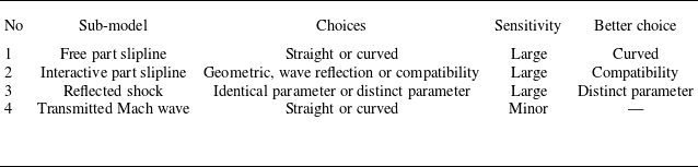
A summary of the sensitivity analysis for the sub-models is presented in table 2. Sub-models of the free part of the slipline, the interactive part of the slipline and the reflected shock have a great influence on the overall accuracy of the Mach reflection model. Specifically, the curved model, compatibility based model and distinct parameter model are the preferred choices for the free part of the slipline, interactive part of the slipline, and reflected shock sub-models, respectively. For the transmitted Mach waves, choice of the straight model or the curved model has little effect on the predicted accuracy.
Sensitivity analysis summary.

The variation of (a) the angle of the characteristic line and (b) the pressure ratio above the slipline for
 $M_{0}=4$
,
 $ \theta _{w}=26^{\circ }$
,
 $g=0.6$
.

4. The variation of the Mach stem height and a calibrated formula
4.1. The linear variation law of Mach stem height and wedge trailing edge height
The linear variation of Mach stem height with wedge trailing edge height has been noted in earlier studies, such as Schotz et al. (Reference Schotz, Levy, Ben-Dor and Igra1997). Bai & Wu (Reference Bai and Wu2021) and Qin et al. (Reference Qin, Shi, Dowell, Pei and Huang2022) validated this relationship numerically under limited conditions, leaving it unclear whether the observed trend represents a specific case or a universal characteristic of Mach reflection.
To address this uncertainty, we conducted a series of systematic numerical simulations of Mach reflection across a broader range of flow and geometric conditions. The variation of Mach stem height with wedge trailing edge height was analysed.
Representative CFD results are presented in figure 18, alongside comparative predictions from the updated theoretical model. The data reveal that across all tested conditions, Mach stem height exhibits a clear linear dependence on wedge trailing edge height. This confirms that the trend is not condition-specific but rather a general feature of shock wave reflection behaviour. Furthermore, the updated model demonstrates excellent agreement with CFD results in capturing this linear trend, including the slope of variation. This confirms that the proposed model offers a reliable predictive capability for the linear dependence of Mach stem height on wedge trailing edge height in Mach reflection configurations.
Although the updated model predicts the slope of the linear variation, it tends to slightly overestimate the absolute value of the Mach stem height. Therefore, we next introduce a calibrated formula based on extensive numerical simulations and the underlying physical trends governing Mach stem height variation.
Comparison of the updated model and CFD results under different conditions: (a)
 $M_{0}=3$
, (b)
 $M_{0}=4$
, (c)
 $M_{0}=5$
.

4.2. Approximate functional forms of the slope
$k$
and intercept
$m$


Extensive CFD results have demonstrated a clear linear relationship between Mach stem height and wedge trailing edge height. To characterise this behaviour, a linear expression is postulated as
 \begin{equation} \frac {H_{T}}{H_{A}}=k(M_{0},\theta _{w})\,g +m(M_{0},\theta _{w}), \end{equation}
where the slope
 $k$
and intercept
 $m$
depend solely on the inflow Mach number
 $ M_{0}$
and the wedge angle
 $\theta _{w}$
.
To accurately derive a fitting formula for Mach stem height, it is essential to first analyse the variation patterns of the slope
 $k$
and intercept
 $m$
. Figures 19 and 20 illustrate the behaviours of
 $k$
and
 $m$
under various conditions, plotted on different planes. The observed trends can be summarised as follows.
-
(i) The slope
$k$
is consistently negative, while the intercept
$m$
remains positive. -
(ii) For a fixed
$M_{0}$
, the slope
$k$
decreases and the intercept
$m$
increases as the wedge angle
$\theta _{w}$
increases. Furthermore, the rates of change for both parameters accelerate with increasing
$\theta _{w}$
. -
(iii) For a fixed wedge angle
$\theta _{w}$
, the slope
$k$
increases and the intercept
$m$
decreases as the Mach number
$M_0$
increases. Furthermore, the rates of change for both parameters gradually diminish with further increases in
$M_0$
.


The variation of (a) slope
 $k$
and (b) intercept
 $m$
with
 $M_0$
for different wedge angles obtained by CFD.

The variation of (a) slope
 $k$
and (b) intercept
 $m$
with
 $\theta _{w}$
for different Mach numbers obtained by CFD.

The slope
 $k$
and the intercept
 $m$
play an important role in the rapid prediction of Mach stem height. To facilitate efficient estimation, approximate functional forms for
 $k$
and
 $m$
are proposed. It is well established, for a fixed specific heat ratio
 $\gamma =1.4$
, that both the slope
 $k$
and the intercept
 $m$
are determined by the inflow Mach number
 $M_{0}$
and the wedge angle
 $\theta _{w}$
. Accordingly, the calibrated formulas are assumed to take the form of a product of two single-variable functions, expressed as
 \begin{equation} \left \{ \begin{array}{l} k(M_{0},\theta _{w})=f_{k1}(M_{0})\times f_{k2}(\theta _{w}), \\[3pt] m(M_{0},\theta _{w})=f_{m1}(M_{0})\times f_{m2}(\theta _{w}). \end{array} \right . \end{equation}
According to figures 19 and 20, the functions
 $f_{k1}(M_{0})$
and
 $f_{m1}(M_{0})$
tend towards zero as the inflow Mach number
 $M_{0}$
approaches infinity for a fixed wedge angle
 $ \theta _{w}$
. Conversely, for a fixed Mach number
 $M_{0}$
,
 $f_{k2}(\theta _{w})$
and
 $f_{m2}(\theta _{w})$
tend towards infinity as
 $\theta _{w}$
approaches the detached angle of the incident shock
 $\theta _{\textit{max}}$
. These functions also vanish when
 $\theta _{w}=\theta ^{(N)}$
, corresponding to the von Neumann condition.
Based on the observed behaviours,
 $f_{k1}$
and
 $f_{m1}$
exhibit characteristics similar to power functions, while
 $f_{k2}$
and
 $f_{m2}$
resemble logarithmic functions. The following assumptions are adopted.
-
(i) When
$M_{0}$
and
$\theta _{w}$
satisfy the von Neumann criterion, both
$k$
and
$m$
vanish, i.e.(4.3)
\begin{equation} \left \{ \begin{array}{l} k=0,\ \theta _{w}=\theta ^{(N)}, \\[3pt] m=0,\ \theta _{w}=\theta ^{(N)}. \end{array} \right . \end{equation}
-
(ii) When
$\theta _{w}$
approaches
$\theta _{\textit{max}}$
, where
$\theta _{\textit{max}}$
denotes the detachment angle of the incident shock and is a function dependent on inflow Mach number, the values of
$k$
and
$m$
diverge:(4.4)
\begin{equation} \left \{ \begin{array}{l} k\rightarrow -\infty ,\ \theta _{w}\rightarrow \theta _{\textit{max}}, \\[3pt] m\rightarrow +\infty ,\ \theta _{w}\rightarrow \theta _{\textit{max}}. \end{array} \right . \end{equation}


Here, infinity
 $\infty$
means very large.
Based on assumptions (4.3)–(4.4), the calibrated functional forms for
 $k$
and
 $m$
are proposed as
 \begin{equation} \left \{ \begin{array}{l} f_{k1}(M_{0})=c_{k1}M_{0}^{c_{k2}}\,{\rm e}^{c_{k3}M_{0}+c_{k4}}, \\[5pt] f_{m1}(M_{0})=c_{k1}M_{0}^{c_{k2}}\,{\rm e}^{c_{k3}M_{0}+c_{k4}}, \end{array} \right . \end{equation}
and
 \begin{equation} f_{k2}(\theta _{w})=f_{m2}(\theta _{w})=\ln\! \left(\frac {\theta _{\textit{max}}-\theta _{w} } {\theta _{\textit{max}}-\theta ^{(N)}}\right)\!. \end{equation}
Using the least squares method and CFD data for
 $M_{0}=2,3,5$
, the coefficients in (4.5) are determined as
 \begin{equation} \left \{ \begin{array}{l} c_{k}=0.59,0.14,-0.15,2.25, \\ c_{m}=-1.31,-0.31,-0.10,1.53. \end{array} \right . \end{equation}
Therefore, the calibrated formulas of the slope
 $k$
and intercept
 $m$
are
 \begin{equation} \left \{ \begin{array}{l} {f_{k1}}({M_0}) = 0.59M_{0}^{0.14}{\,{\rm e}^{ - 0.15{M_0} + 2.25}}, \\[5pt] {f_{m1}}({M_0}) = - 1.31M_{0}^{ - 0.31}{\,{\rm e}^{ - 0.10{M_0} + 1.53}}. \end{array} \right . \end{equation}
The normalised Mach stem height can be predicted from
 \begin{equation} H_{T}/H_{A}=\{ f_{k1}({M_0})\,g+f_{m1}({M_0})\} \ln\! \left(\frac {\theta _{\textit{max}}-\theta _{w} }{\theta _{\textit{max}}-\theta ^{(N)}}\right)\!. \end{equation}
The first factor,
 $f_{k1}({M_0})\,g+f_{m1}({M_0})$
, describes the influence of the geometric parameter
 $g$
and is negative. The second factor,
 $\ln (({\theta _{\textit{max}}-\theta _{w} })/({\theta _{\textit{max}}-\theta ^{(N)}}))$
, isolates the influence of the wedge angle
 $\theta _w$
. This form is derived from the boundary conditions, and is also negative for all valid Mach reflection configurations. This negativity arises because the wedge angle
 $\theta _w$
satisfies
 $\theta _N \lt \theta _w \lt \theta _{\textit{max}}$
for such configurations, which yields a ratio inside the logarithm that is positive but less than 1. This factorised form facilitates the independent quantification of the contributions of
 $M_0$
and
 $\theta _w$
, improving the parametric analysis capability. The valid range is
 $M_0=2{-}5$
.
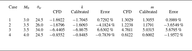
Comparion of the slope
 $k$
and intercept
 $m$
obtained from the calibrated formula and CFD.

4.3. Analyses and results
The slope
 $k$
and intercept
 $m$
can be quantitatively predicted using the calibrated expressions from (4.2) and (4.6)–(4.8). Figure 21 presents a comparative analysis among three approaches: the calibrated formula, the updated model and the CFD results under
 $M_{0}=5$
. It can be seen that the
 $k$
and
 $m$
values given by the updated model are already quite accurate, but the results given by the calibrated model are basically consistent with the numerical results. Additional comparisons under varying conditions are provided in table 3 and figure 22, which further demonstrate that the calibrated formula closely agrees with the CFD data.
Furthermore, figure 23 shows a comparison of the CFD results and predictions from the calibrated formula under
 $M_{0}=2.2$
,
 $M_{0}=3.5$
and
 $M_{0}=4$
. It can be seen that the accuracy of the calibrated formula shows good agreement with the results obtained by CFD.
In general, these results confirm that the calibrated formula (4.8) provides sufficient accuracy for predicting both
 $k$
and
 $m$
, and (4.9) provides sufficient accuracy for predicting for Mach stem height.
Comparison of the slope
 $k$
and intercept
 $m$
obtained from the calibrated formula, updated model and CFD for
 $M_{0}=5$
.

Comparison of the slope
 $k$
and intercept
 $m$
obtained from the calibrated formula and CFD.

The results obtained by the calibrated formula under different conditions: (a)
 $M_{0}=2.2$
, (b)
 $M_{0}=3.5$
, (c)
 $M_{0}=4$
.

5. Concluding remarks
This paper systematically investigates the prediction accuracy of the Mach stem height in supersonic shock wave reflection.
An updated model has been developed. Compared with the model of Bai & Wu (Reference Bai and Wu2017), the updated model has some significant differences. For example, Bai & Wu (Reference Bai and Wu2017) assume a uniform pressure gradient along the transmitted Mach wave and approximate its shape as a straight line, while the updated model considers the transmitted Mach wave as a small curvature curve and assumes that its flow parameters satisfy the compatibility relation corresponding to the
 $C_{-}$
family; Bai & Wu (Reference Bai and Wu2017) hypothesised that transmitted Mach waves will reflect and generate compression waves above the slipline, while the updated model suggests that the flow parameters above the slipline and the parameters at the triple point satisfy the compatibility relation corresponding to the
 $C_{0}$
family.
We adopted the updated model as the benchmark to perform sensitivity analysis on several sub-models corresponding to typical flow structures in Mach reflection. It is found that the assumption that the flow above the slipline conforms to the
 $C_0$
compatibility relation is more consistent with flow physics, enabling the updated model to better capture the linear variation slope of Mach stem height with wedge trailing edge height. Additionally, the curve assumption for the free part of the slipline and the distinct parameter sub-model for the interactive part of the reflected shock can improve the model accuracy to a certain degree, while the transmitted Mach wave is basically close to a straight line.
Moreover, by combining asymptotic reasoning with high-fidelity numerical data, a linear scaling law for the Mach stem height was established. This law takes the form of a factorised function that decouples the independent contributions of the inflow Mach number
 $M_{0}$
and the wedge angle
 $\theta _{w}$
, with the normalised Mach stem height
 $H_{T}/H_{A}$
expressed as the product of an
 $M_{0}$
-dependent term and a
 $\theta _{w}$
term. Valid for
 $ M_{0}$
in the range
 $M_{0}=2{-}5$
, this scaling law achieves a maximum relative error of less than 5 % compared to the CFD results, providing more accurate predictions over a wide parameter space compared to existing theoretical models. However, the calibrated model has been obtained using CFD data with
 $\theta _{w}$
slightly above the von Neumann condition. When
 $ \theta _{w}\rightarrow \theta ^{(N)}$
, the Mach stem height is vanishing, requiring perhaps a large number of grid points along the Mach stem. The behaviour of the Mach stem height with
 $\theta _{w}\rightarrow \theta ^{(N)}$
deserves further study.
Acknowledgements
The authors are grateful to the referees for their useful and valuable comments that helped to improve the paper.
Funding
This work was supported by the Natural National Science Foundation of China (nos 12472232 and 52192632) and Beihang University Young Elite Talent Support Program (501XYGG2025105003).
Declaration of interests
The authors report no conflict of interest.
Appendix A. Numerical simulation for Mach reflection
The numerical results are obtained, on a structured grid, by solving the compressible Euler equations for a perfect gas using the well-known second-order Roe scheme. As usual, an unsteady approach is used to converge to the steady-state solution, so we need an initial condition. A uniform initial condition with the flow parameters set to the inlet values is used, which is found to give regular reflection (RR) in the RR domain and double solution domain, and Mach reflection (MR) in the MR domain. In the double solution domain, we first use a low inflow Mach number (where the reflection is in the MR domain) to obtain steady-state results, then adjust the inflow Mach number to the desired one to obtain an MR.
To ensure the accuracy of the CFD results, simulations were conducted using various grid densities for
 $g=0.55$
, with
 $M_{0}=4$
,
 $ \theta _{w}=24^{\circ }$
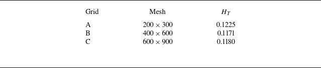
. The Mach stem heights corresponding to each grid density are presented in table 4. It can be observed that the results obtained with grids B and C are very similar, suggesting that the solution with grid C may be used as a reference. When compared to this reference, grid A shows a relative error of approximately 3.4 %, while grid B exhibits a smaller error of approximately 0.8 %. Therefore, grid B is selected for further analyses. Additionally, 80 grid points are placed along the Mach stem, between the reflecting surface and the triple point, to ensure computational accuracy.
The Mach stem height under different grid densities.

Grid independence. The Mach number contours are obtained by CFD with different grids for
 $M_0=4, \theta_w=24^{\circ}$
and
 $g=0.55$
: (a) flow structure; (b) enlarged view.

Definitions of the parameters across (a) an oblique shock and (b) an expansion fan.

Appendix B. Classical shock relations and Prandtl–Meyer relations
Across an oblique shock wave, as depicted in figure 25(a), the downstream flow parameters (with subscript
 $d$
) are related to the upstream flow parameters (with subscript
 $u$
) by classical shock relations
 \begin{equation} M_{d}=f_{M}\left ( M_{u},\beta _{ud}\right ) ,\quad p_{d}=p_{u}\,f_{p}\left ( M_{u},\beta _{ud}\right ) ,\quad \rho _{d}=\rho _{u}\,f_{\rho }\left ( M_{u},\beta _{ud}\right )\!, \end{equation}
where the abbreviations are
 \begin{equation} \left \{ \begin{array}{l} f_{M}(M,{\beta )}=\sqrt {\dfrac {\left ( \gamma -1\right ) {M}^{2}+2}{2\gamma {M} ^{2}\sin^{2}{\beta }-\left ( \gamma -1\right ) }+\frac {2{M}^{2}{\cos }^{2}{ \beta }}{\left ( \gamma -1\right ) {M}^{2}{\sin }^{2}{\beta }+2}} ,\\[12pt] f_{p}(M,{\beta )}=1+\frac {2\gamma }{\gamma +1}\left ( {M}^{2}\sin^{2}{ \beta }-1\right )\!, \\[9pt] f_{\rho }\left ( M,\beta \right ) =\dfrac {\left ( \gamma +1\right ) {M}^{2}{\sin } ^{2}{\beta }}{2+\left ( \gamma -1\right ) {M}^{2}\sin^{2}{\beta }}.\end{array} \right . \end{equation}
Here, the shock angle
 $\beta _{ud}$
is related to the flow deflection angle across the shock
 $\vert \theta _{ud}\vert =\vert \theta _{d}-\theta _{u}\vert$
by the shock angle relation
 \begin{equation} \left \{ \begin{array}{l} \left \vert \theta _{ud}\right \vert =f_{\theta }\left ( M_{u},\beta _{ud}\right )\!, \\ f_{\theta }({M,\beta })=\arctan \dfrac {2\left ( {M}^{2}\sin^{2}{\beta } -1\right ) }{\left ( {M}^{2}\left ( \gamma +\cos \left ( {2\beta }\right ) \right ) +2\right ) \tan {\beta }}. \end{array} \right . \end{equation}
Inside the unperturbed expansion fan, as depicted in figure 25(b), the classical Prandtl–Meyer relation is satisfied:
 \begin{equation} \nu (M)-\nu (M_{1})=\theta -\theta _{1}, \end{equation}
where
 $\nu (M)=\sqrt {( {\gamma +1})/({\gamma -1}})\arctan \sqrt {( ({\gamma -1})/({\gamma +1}))(M^{2}-1)}-\arctan{} \sqrt {M^{2}-1}$
is the Prandtl–Meyer function. The pressure and density inside the unperturbed expansion fan satisfy the isentropic flow relations
 \begin{equation} \frac {p}{p_{1}}=\left ( \frac {\vartheta (M_{1})}{\vartheta (M)}\right ) ^{ {\gamma }/({\gamma -1})},\quad\frac {\rho }{\rho _{1}}=\left ( \frac {\vartheta (M_{1})}{\vartheta (M)}\right ) ^{{1}/({\gamma -1})}, \end{equation}
where
 $\vartheta (M)=1+(( {\gamma -1})/{2})M^{2}$
.