Introduction
Radiotherapy (external beam radiation therapy) represents a cornerstone of cancer treatment in a wide range of clinical cases. Its fundamental objective is to deliver a sufficiently high radiation dose to the targeted tumor while minimizing exposure to the surrounding healthy tissue. As technological advances have enabled photons, protons, and heavy ions to be delivered with ever-increasing precision and dose accuracy, the motion of the target volume has emerged as a critical factor in treatment quality. This is particularly relevant for tumors located in the abdomen and lungs, where respiratory motion can cause substantial displacement of the target. A common strategy to account for such motion is to incorporate target volume displacement into treatment planning by enlarging the irradiation field accordingly. However, this approach inevitably increases the radiation dose to healthy tissue, thereby elevating the risk of adverse side effects. A more targeted alternative involves tracking the motion of the tumor itself, adjacent anatomical structures, or the body surface, allowing irradiation to be gated to a specific phase of the respiratory cycle. To support accurate treatment planning, a 4D CT (X-ray computed tomography) is acquired, capturing the tumor position across multiple phases of the respiratory cycle. Crucially, respiratory motion of the body surface must be monitored simultaneously during CT acquisition to ensure spatial correspondence between the imaging data and the patient’s breathing state.
One approach to compensate for tissue motion and enhance existing systems is to extract the patient’s body surface and compare it to a previously generated 4D treatment plan. This principle is generally known as surface-guided radiation therapy (SGRT); see [Reference Darréon, Massabeau, Geffroy, Maroun and Simon1, Reference Freislederer, Kugele, Ollers, Swinnen, Sauer, Bert, Giantsoudi, Corradini and Batista2] for overviews. State-of-the-art SGRT is dominated by camera-based systems (e.g., Align RT [Vision RT], C-RAT [Catalyst RT], or Identify [Varian]) that rely on stereo vision techniques. These systems typically achieve high positioning accuracies below 1 mm and rotational accuracies of about 1 $^\circ$ [Reference Waghorn3, Reference Freislederer, Batista, Öllers, Buschmann, Steiner, Kügele, Fracchiolla, Corradini, de Smet, Moura, Perryck, Dionisi, Nguyen, Bert and Lehmann4]. SGRT could be combined with deep inspiration breath hold, and major clinical applications include breast cancer treatments [Reference Rudat, Zhao, Wang, Zhang and Shi5–Reference Kadhim, Haraldsson, Kügele, Enocson, Bäck and Ceberg7], cranial treatments [Reference Flores-Martinez, Cerviño, Pawlicki and Kim8], and thoracic irradiation [Reference Nguyen, Reinoso, Farah, Yossi, Lorchel, Passerat, Louet, Pouchard, Khodri and Barbet9]. These systems are well established in routine clinical workflows and demonstrate high robustness and reliability. Their main limitations, however, include high equipment costs and reduced performance with darker skin tones, clothing, or thermoplastic masks.
In parallel, radar-based approaches have been investigated as alternative sensing modalities for respiratory gating in radiotherapy; cf. [Reference Pepa, Sellaro, Marchesi, Caracciolo, Serra, Orlandi, Baroni and Pella10] for an overview. Existing contributions primarily focus on tracking motion at isolated anatomical points or small regions of interest using either single-channel radars or small MIMO (multiple input multiple output) devices; see [Reference Gu, Li, Zhang, Fung, Torres, Jiang and Li11–Reference Kosaka, Kubo, Matsumoto, Nakamura and Monzen15] for examples. Beyond radiotherapy, radar-based estimation of respiratory movement and heartbeat is a very active field in radar signal processing; cf. [Reference Paterniani, Sgreccia, Davoli, Guerzoni, Di Viesti, Valenti, Vitolo, Vitetta and Boriani16, Reference Frazao, Pinho and Albuquerque17] and references therein. Although many studies report millimeter-level accuracy, they do not provide surface reconstructions. For further applications of microwave/radar sensors in the medical context, see [Reference Zhang, Liu, Cheng, Li, Xu, Huang, Zhan, Bo, Xia and Xu18–Reference Origlia, Rodriguez-Duarte, Vasquez, Bolomey and Vipiana20].
Outside the medical context, high-precision phase-based techniques have been explored extensively, e.g., in automotive and non-destructive testing, demonstrating high ranging accuracy [Reference Piotrowsky, Jaeschke, Kueppers, Siska and Pohl21–Reference Antes, Kollár, Zwick and Nuss23], ego-motion estimation of moving platforms [Reference Yuan, Zhu, Fioranelli and Yarovoy24–Reference Stockel26], or the characterization of diffraction effects [Reference Schlosser, Froehly, Herschel and Pohl27]. Furthermore, surface reconstruction methods were introduced in [Reference Pohle, Barowski, Jebramcik and Rolfes28–Reference Pawliczek, Herschel and Pohl30], typically combining amplitude and phase information from reconstructed radar images. To compensate for phase ambiguities, path-following unwrapping approaches ([Reference Pawliczek, Herschel and Pohl29, Reference Pawliczek, Herschel and Pohl30], see also [Reference Herráez, Burton, Lalor and Gdeisat31]) are commonly used. In contrast, we adopt a Fourier-based phase unwrapping algorithm [Reference Ghiglia and Romero32], which is computationally efficient and path-independent. We also refer to [Reference Ghiglia and Pritt33] for an overview. We note that prior results consider static surfaces, limiting tracking of dynamic surface changes. To address this, we introduce an additional temporal unwrapping stage.
In summary, existing radar-based solutions either lack full 3D surface coverage or do not incorporate the temporal phase evolution required for dynamic tracking. The approach presented in this work bridges these gaps by combining: (i) a real-aperture ultra-wideband (UWB) imaging system operating from 6.5 to 10.5 GHz and (ii) an algorithmic scheme featuring a weighted Fourier-based spatial unwrapping and a temporal unwrapping. The general design is validated by simulations and measurements.
The remainder of the paper is organized as follows. The second section introduces the imaging system, followed by the reconstruction and tracking algorithms in the third section. The fourth section presents the measurement phantom designed for validation. Finally, the fifth section validates the system design and algorithmic approach through simulations and measurement results.
An earlier version of this paper was presented at EuMW 2025 and was published in its Proceedings [Reference Froehly, Nowok, Shoykhetbrod, Brauns and Wallrath34].
Radar imaging system
Radar module
The measurement system used in this study is based on a commercially available radar front-end manufactured by Vayyar Imaging Ltd, cf. also [Reference Cetinkaya, Nowok and Herschel35, Reference Baqué, Vignaud, Wasik, Castet, Herschel, Cetinkaya and Brandes36] for their use in non-destructive testing and security applications. The module incorporates a total of 40 antenna elements. These elements are mounted on a rectangular printed circuit board (PCB) with physical dimensions of 20 cm by 20 cm. The antennas are positioned in an equidistant, grid-like arrangement, ensuring uniform spatial sampling across the aperture (see Figure 1). In the configuration of the module, pairs of opposing antenna elements are designated as either transmit (Tx) or receive (Rx) units. In addition, the antennas located at the four corners of the board are configured to perform both transmit and receive operations. As a consequence, the system provides a total of 22 Tx channels and 22 Rx channels, enabling flexible and diverse measurement configurations.
Used module with Tx and Rx antenna array.

The radar module operates at a nominal center frequency of 8.5 GHz and supports a signal bandwidth of 4 GHz. This results in a free-space wavelength of approximately 3.53 cm at the center frequency. The transmitted waveform is a classical step-frequency continuous wave (SFCW) modulation scheme. The antenna characteristics yield a 3 dB beamwidth of approximately 100 $^\circ$, providing a wide angular coverage suitable for applications requiring a large field of view. To manage the multiple transmit channels, the system employs a time-division multiplexing strategy. The switching interval between two consecutive Tx activations is 490 µs while maintaining sufficient temporal separation to avoid inter-channel interference.
Complete system
The complete radar system architecture consists of three individual radar modules of the type described in the previous subsection (see Figure 4). To ensure coherent waveform generation and synchronized operation across all modules, a dedicated control and signal-generation unit is employed. This additional unit generates the global reference clock signal, provides the GPIO (general-purpose input/output) based control signals for coordinated time-division multiplexed operation, and synthesizes the high-frequency (HF) excitation signal used by the radar front-ends.
The distribution of these signals is accomplished through a combination of specialized splitter boards. The clock and GPIO lines are routed together via dedicated distribution boards to each of the three radar modules. In contrast, the HF signal is distributed using a Wilkinson-based power divider network. The HF chain begins with an active Wilkinson divider that initializes the power distribution stage, after which subsequent splitting steps are performed using passive Wilkinson dividers to route the signal to all modules while maintaining phase coherence and impedance matching.
The mechanical configuration of the system is designed to enable flexible aperture control,. The central radar module is mounted parallel to the torso surface. The two outer modules are positioned symmetrically around the central unit and can be tilted by an inclination angle adjustable between 0 $^\circ$ and 45
 $^\circ$. This adjustable geometry allows the aperture to be adapted to the object’s spatial extent, thereby optimizing angular coverage and improving reconstruction performance in applications where a variable viewpoint is advantageous.
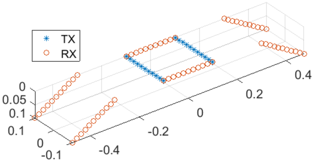
For this proof of concept, the central module employs all of its transmit (Tx) and receive (Rx) antenna channels, whereas the two outer modules are operated in receive-only mode with their Tx antennas disabled; see Figure 2. In this configuration, the system is capable of generating measurement frames at a rate of up to 62.5 Hz. We note that this design choice is primarily motivated by showing that even a comparatively small virtual aperture of approximately 60 cm  $\times$ 20 cm enables one to obtain high accuracies for the surface reconstruction. In fact, the full transmit–receive configuration has been proven to be of almost no influence on the surface reconstruction (cf. also the remarks in Section “Simulation results”).
Distribution of transmitter (blue) and receiver (red).

Surface reconstruction and tracking
The surface reconstruction follows the principles of phase-based radar signal processing, and thus, can achieve high accuracy but must cope with phase ambiguity. We briefly recall the key ideas using the SFCW signal model. Let  $f[m] = f_0 + (m-1) \Delta f$,
 $m=1,\dots,M$, denote the discrete frequency steps of the sweep. The measured radar signal for a single point scatterer at range
 $R_0$ is
 \begin{equation}
s[m] = \exp \bigg\{- 2\pi j f[m] \frac{2 R_0}{c_0} \bigg\} ,
\end{equation}
where  $c_0$ is the speed of light in vacuum. Here, we assume a quasi-monostatic configuration. Then a suitable discretization of the range variable is given by
 \begin{equation}
R[k] = \frac{(k-1)}k \frac{c_0}{2\Delta f} .
\end{equation}
In this case, the matched filter corresponds up to a phase correction factor (and a constant) to the inverse discrete Fourier transform (IDFT):
 \begin{equation}
\mathrm{MF}[k]
= \sum_m s[m] \exp \bigg\{2\pi j f[m] \frac{2 R[k]}{c_0}\bigg\}
\end{equation}
 \begin{equation}
\sim \exp \bigg\{2\pi j f_0 \frac{2 R_0}{c_0}\bigg\} \cdot \mathrm{IDFT}\{s\} [k].
\end{equation}
A short calculation yields
 \begin{equation}
\mathrm{MF}[k] \sim q(R - R[k]) \exp \bigg\{- 2 \pi j f_c \frac{2 (R_0 - R[k]) }{c_0}\bigg\} ,
\end{equation}
where  $q$ is a sinc-like peak function and
 $f_c$ denotes the center frequency. In particular, the phase
 $\phi[k]$ for a certain range bin
 $R[k]$ is proportional to the mismatch between the range bin and the true range
 $R_0$:
 \begin{equation}
R_0 - R[k] = - \frac{\phi[k]}{2\pi} \cdot \frac{\lambda_c }{2} .
\end{equation}
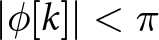
Here  $\lambda_c$ denotes the wavelength corresponding to the center frequency. Due to the phase ambiguity, this linear relation is only valid if
 $R[k]$ is located near the true range, i.e., if
 $|\phi[k]| \lt \pi$ or equivalently
 $|R_0 - R[k]| \lt \lambda_c/4$.
This idea generalizes to aperture-based imaging [Reference Pawliczek, Herschel and Pohl29, Reference Pawliczek, Herschel and Pohl30], where a physical or synthetic aperture is formed and conventional backprojection serves as the matched filter. One first specifies an initial approximate surface  $(x,y,z_0(x,y))$ and reconstructs the image values along this surface. The corresponding phase values
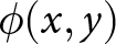 $\phi(x,y)$ then obey
 \begin{equation}
\mathrm{d}z(x,y) \;=\; -\,\frac{\phi(x,y)}{2\pi}\cdot\frac{\lambda_c}{2},
\end{equation}
where 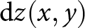 $\mathrm{d}z(x,y)$ denotes the mismatch in range direction between the approximate and the actual surface. Then Eq. (7) serves as a correction to refine the surface.
This approach requires a highly accurate initial estimate of the actual surface, with deviations not exceeding  $\frac{\lambda}{4}$. To compensate for a few number of points outside the unambiguous range, a spatial phase unwrapping algorithm is applied. However, during respiratory motion, the initial estimate may deviate beyond this bound, and while spatial unwrapping still yields a consistent surface, its absolute position may be incorrect. To address this, an additional temporal unwrapping algorithm is applied, requiring only that the displacement between two subsequent frames remains below
 $\frac{\lambda}{4}$. If the initial estimate is inaccurate, the result is a spatially and temporally consistent surface with a fixed offset relative to the true surface.
The main algorithm is presented in detail in the following. A flow chart is shown in Figure 3. Each step in the flow chart is accompanied by an image illustrating the intermediate result.
Flow chart for the surface extraction.

Figure 3 Long description
.The flow chart consists of six blocks connected by labeled arrows. The first block, “Measurement Data”, contains no image. An arrow labeled “Matched Filter” leads from it to the second block, “2D Image”, which displays a grayscale image in the X-Y plane. Along this arrow, a second arrow merges in from a separate block labeled “2D Approximated Surface”, which shows a grayscale mesh of a torso with an approximated surface outline. From the “2D Image” block, an arrow labeled “Phase Extraction” leads to the “Phase Values” block, showing a corresponding X-Y image of the extracted phase values. An arrow then leads to the “Unwrapped Phase Values” block, showing the same region after phase unwrapping. A final arrow leads to the last block, which shows a mesh of the torso with the extracted phase overlaid on its surface. The three intermediate X-Y images (“2D Image”, “Phase Values”, and “Unwrapped Phase Values”) all show the same field of view, spanning X from negative 0.22 m to 0.22 m and Y from negative 0.15 m to 0.15 m.
Before data acquisition, one selects a first 2D approximate surface. The location of this surface may be known a priori (e.g., from measuring the distance between radar and torso) or estimated using the imaging system itself. To this end, a 3D image is reconstructed from an initial data acquisition. Subsequently, we identify the amplitude peak along the range dimension using either a finely sampled voxel grid or interpolation. Then the surface is regularized via Gaussian smoothing and (if needed) fitted with a polynomial in  $x,y$. We note that this surface remains fixed throughout the measurement, reflecting the torso’s small respiratory motion.
Once the approximated surface is fixed, we reconstruct the image values and then calculate the phase values. For phase unwrapping, we employ the Fourier-based method of Chap. 5 in [Reference Ghiglia and Pritt33]. Let us go into detail: let 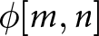 $\phi[m,n]$ denote the wrapped phase values on the approximated surface. The unwrapped phase
 $\psi$ is defined as the minimizer of the functional
 \begin{align}\notag
J[\psi] &=\sum_{m,n} \bigl|\psi[m,n] - \psi[m-1,n] - \Delta^{(1)}_{m,n} \bigr|^2
\\
&\; + \sum_{m,n}
\bigl|\psi[m,n] - \psi[m, n-1] - \Delta^{(2)}_{m,n} \bigr|^2\to \mathrm{min} ,\end{align}
where
 \begin{equation}
\Delta^{(1)}_{m,n} = ( \phi[m,n] - \phi[m-1,n] ) \mod(-\pi, \pi)
\end{equation}
 \begin{equation}
\Delta^{(2)}_{m,n} = ( \phi[m,n] - \phi[m,n-1] ) \mod(-\pi, \pi) .
\end{equation}
Here 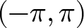 $(-\pi, \pi) $ denotes the unambiguous range of the phase values. Then one may show that the minimizer
 $\psi$ satisfies the discrete Laplace equation
 \begin{equation}
\psi[m+1,n] - 2 \psi[m,n] + \psi[m - 1, n] = \Delta^{(1)}_{m,n}
\end{equation}
 \begin{equation}
\psi[m,n+1] - 2 \psi[m,n] + \psi[m , n-1] = \Delta^{(2)}_{m,n}
\end{equation}
as well as
 \begin{equation}
\psi[2,n] - \psi[1,n] = \Delta^{(1)}_{1,n},
\end{equation}
 \begin{equation}
\psi[m,2] - \psi[m,1] = \Delta^{(2)}_{m,1},
\end{equation}
 \begin{equation}
\psi[M,n] - \psi[M-1,n] = \Delta^{(1)}_{M,n},
\end{equation}
 \begin{equation}
\psi[m,N] - \psi[m,N-1] = \Delta^{(2)}_{m,N}.
\end{equation}
This system is diagonalized by the discrete cosine transform, enabling an efficient solver. For surface reconstruction, however, it is necessary to introduce amplitude-dependent weights, and thus, a conjugate-gradient algorithm has to be applied. For efficient computation, the solution operator of (11)–(16) is used as a preconditioner, cf. also [Reference Ghiglia and Pritt33]. This also concludes the steps depicted in Figure 3.
Now we assume that for each time  $t_k$ we have phase values
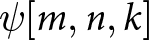 $\psi[m,n,k]$ after spatial unwrapping. In a next step, we calculate the torso motion by unwrapping across the temporal index
 $k$. Specifically, we seek
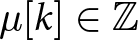 $\mu[k] \in \mathbb{Z}$ such that
 \begin{equation}
\widetilde{\psi}[m,n,k] = \psi[m,n,k] + 2\pi \cdot \mu[k]
\end{equation}
gives the “true” phase values after temporal unwrapping. Taking into account the already calculated values 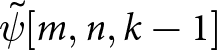 $\widetilde{\psi}[m,n,k-1]$ at time
 $t_{k-1}$, we set
 \begin{equation}
\mu[k] = \Big\lfloor \frac{1}{2\pi} \sum_{m,n} \gamma_{m,n} (\psi[m,n,k] - \widetilde{\psi}[m,n,k-1]) \Big\rceil,
\end{equation}
where  $\lfloor \cdot \rceil$ denotes the rounding operator. Here
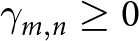 $\gamma_{m,n} \ge 0$ are weights chosen according to the magnitude of the image cells satisfying
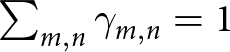 $\sum_{m,n} \gamma_{m,n} = 1$. In this way, we are able to estimate the torso location at each temporal index
 $k$.
Torso phantom
To evaluate the system’s performance under controlled and repeatable conditions, a torso phantom was constructed. This allows systematic testing without involving a human participant and avoids the practical and ethical considerations normally associated with human-subject experiments. In addition, the use of a phantom enables identical measurement conditions to be reproduced across multiple experimental runs.
The phantom is based on a medical ventilation training manikin (Ambu), depicted in Figures 4 and 10(a). The manikin incorporates an internal flexible airbag that serves as a lung analog and generates chest motion representative of a respiration cycle. Due to the plastic materials used in the manikin’s construction, its electromagnetic properties differ substantially from those of human tissue. To reduce this mismatch and obtain a more representative electromagnetic response, copper foil was applied to the inner surface of the manikin; cf. also the modeling of the torso surface for simulation purposes in Section “Simulation results.”
UWB system setup (with measurement phantom).

Periodic actuation of the internal airbag was achieved through a microcontroller-based setup. The microcontroller activated and deactivated the air pump according to predefined upper and lower pressure thresholds measured by an integrated pressure sensor. These thresholds allowed the inhalation and exhalation amplitudes to be precisely defined. An adjustable mechanical inlet valve was incorporated into the pump assembly to regulate airflow. By setting the valve opening, the airflow rate – and consequently the time required to reach the upper pressure limit during inflation – could be controlled. When the pump was switched off, the same valve position determined the deflation airflow and thus the duration of exhalation. This configuration made it possible to independently adjust both the timing and amplitude of the breathing cycle and to reproduce specific respiration profiles with sufficient accuracy and repeatability. An overview of the pump, valve assembly, and sensor integration used for airflow regulation is shown in Figure 5.
Experimental setup for generating periodic inflation of the torso phantom, including the air pump, pressure sensor, microcontroller unit, and adjustable inlet valve.

Figure 5 Long description
The photograph shows the electronic control unit for the phantom inflation setup. Five components are labeled directly on the image: the PSU is positioned above the pump; to the right of the PSU are the voltage regulators; below the voltage regulators is the microcontroller ($\mu$Controller); below that is the pressure sensor; and in the lower left of the image is the valve.
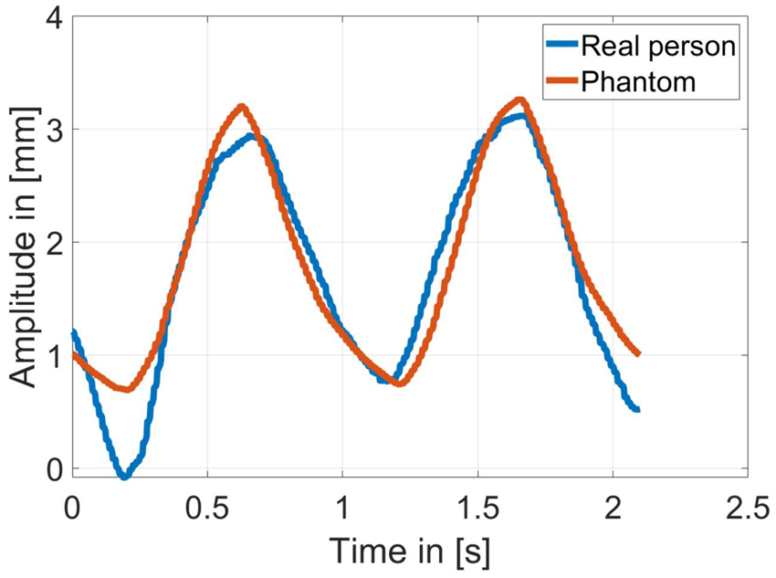
To assess the fidelity of the generated chest motion, measurements from a real person were acquired and compared with those obtained from the phantom under identical breathing-cycle settings. Chest displacement was captured using the harmonic tag system, which is also employed in Section “Measurement results” for validation purposes. The comparison shown in Figure 6 demonstrates that both the timing and amplitude of the phantom’s breathing cycle closely follow the respiration pattern of the human subject. The close alignment of the waveforms confirms that the phantom reproduces human-like chest movement with high accuracy and is therefore suitable for controlled and repeatable validation experiments.
Chest-displacement waveforms of a human subject and the torso phantom, illustrating the correspondence in breathing motion.

Figure 6 Long description
The plot shows two chest-displacement waveforms over time. The horizontal axis is labeled “Time” in seconds, ranging from 0 to 2.5 s. The vertical axis is labeled “Amplitude” in millimeters, ranging from 0 to 4 mm. Two curves are plotted: the human subject’s chest displacement in blue and the torso phantom’s chest displacement in red. Both curves show a periodic, wave-like pattern with closely matching amplitude, frequency, and phase, indicating a close correspondence between the human breathing motion and the phantom’s motion.
Results
Simulation results
We first investigate the accuracy of the proposed approach via simulations with two torso models (male and female), shown in Figure 7.
Models of female and male torso used for simulations in Ansys HFSS.

The female torso is an adapted version (cut and aligned) of “Female Torso” by Kevin Ruiz [Reference Ruiz37] which is licensed under CC BY 4. The male torso corresponds to the phantom in Section “Torso phantom,” which was scanned using the optical 3D scanner Artec Spider in order to create an STL file. The STL file of each torso and the antenna setup were loaded in Ansys HFSS and simulations using SBR+ have been carried out. We modeled the skin as a perfect electric conductor (PEC), which is justified by the strong reflection caused by the high permittivity and conductivity of the human skin in the considered frequency band. More precisely, using the publicly available data in [Reference Foundation38], we observe a relative electric permittivity of 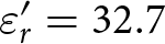 $\varepsilon_r' = 32.7$ (real part), and a conductivity of
 $\sigma = 6.35~\textrm{S}~\textrm{m}^{-1}$ at a frequency of
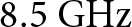 $8.5~\textrm{G}\textrm{Hz}$. This yields a relative complex permittivity of
 \begin{equation}
\varepsilon_r = \varepsilon_r' + \varepsilon_0^{-1} \frac{\sigma}{2\pi f} = 32.7 + j 10.57
\end{equation}
and a refractive index of  $n = 5.79 + j 0.91$. Here
 $\varepsilon_0$ denotes the electric permittivity in vacuum. For the Fresnel reflection coefficients at the air-medium interface, we have for TE and TM polarization
 \begin{equation}
r_{\mathrm{TE}} = \frac{\cos \theta_i - n \cos \theta_t}{\cos \theta_i + n \cos \theta_t}
\end{equation}
 \begin{equation}
r_{\mathrm{TM}} = \frac{n \cos \theta_i - \cos \theta_t}{n \cos \theta_i + \cos \theta_t},
\end{equation}
where  $\theta_i$ denotes the angle of incidence and
 $\theta_t$ denotes the angle of transmission. For normal incidence angle, this reduces to
 \begin{equation}
r_{\mathrm{TE}} = r_{\mathrm{TM}} = - \frac{n - 1}{n + 1}
= - 0.7118 \cdot e^{0.055j} .
\end{equation}
This yields a phase offset of 0.055 rad compared to a PEC boundary and via Eq. (6) this implies a range error of 154.47 µm relative to the true surface, which is negligible in view of the subsequent results. Hence, modeling the surface as PEC constitutes a good approximation of the actual torso.
The imaging and surface reconstruction results for both models are shown in Figure 8.
Plots (a), (c), (e) correspond to the female torso, while (b), (d), (f) show the male torso. The maximum projections of the 3D images are shown in Figure 8(a) and (b). In both cases, the chest region is visible; however, the resolution is rather low due to the chosen frequency range. The reconstructed surfaces obtained with the proposed algorithm are shown in Figure 8(c) and (d). We note that the initial surface for the phase extraction was obtained by a previous amplitude-based surface calculation. At first glance, the male torso surface closely matches the true surface, whereas the female torso already exhibits a somewhat poorer fit. This is confirmed by the error distributions in Figure 8(e) and (f): the male torso shows a qualitatively low error, while the female torso exhibits larger errors, particularly in the breast region. The corresponding root mean square (RMS) errors are shown in Table 1.
Results for female (a), (c), (e) and male (b), (d), (f) torso model; (a) and (b) show the maximum projection of the 3D image; (c) and (d) show the torso together with the reconstructed surfaces; (e) and (f) show the absolute error of the surface reconstruction.

Figure 8 Long description
Six panels compare male (A, C, E) and female (B, D, F) torso models. Panels A and B show maximum-projection heatmaps of the 3D amplitude images in grayscale, with axes labeled “X” and “Y” in meters and a color scale from minus 25 dB (black) to 0 dB (white); the central regions appear brighter, indicating higher intensity. Panels C and D show 3D surface plots with axes labeled “X”, “Y”, and “Z” in meters, displaying the torso as a gray mesh overlaid with a colored reconstructed surface, indicating a good fit between the reconstructed and true surface. Panels E and F show phase error maps with axes labeled “X” and “Y” in meters and a color scale labeled “Error” in millimeters, ranging from 0 mm (blue) to 6 mm (yellow); the outer regions, which are not part of the relevant area, appear yellow, while the central, relevant region shows near-uniform blue and green values for the male torso, indicating a good fit, whereas the female torso shows mostly green with occasional patches of blue, yellow, and orange, indicating a somewhat less accurate fit.
RMS error distribution

Table 1 Long description
Table 1 lists RMS error values in millimeters for four torso models - male, female, female (breast only), and female (stomach only) - across three error measures: absolute phase error, relative phase error, and amplitude error. For the male model, the values are 1.81 mm, 0.94 mm, and 6.00 mm, respectively. For the female model, they are 3.47 mm, 1.47 mm, and 6.32 mm. For the female (breast only) model, they are 2.51 mm, 1.32 mm, and 5.48 mm. For the female (stomach only) model, they are 1.16 mm, 0.67 mm, and 9.29 mm. Across all models, the absolute phase error ranges from 1.16 mm to 3.47 mm and the relative phase error ranges from 0.67 mm to 1.47 mm, both lowest for the female (stomach only) model. The amplitude error ranges from 5.48 mm to 9.29 mm, with the female (stomach only) model showing the highest value and the female (breast only) model the lowest.
The first column reports the RMS error for the phase-based surface reconstruction: 1.81 mm for the male torso and 3.47 mm for the female torso. Since we are primarily interested in motion, we also report the relative error (after subtracting the mean), yielding 0.94 mm for the male and 1.47 mm for the female torso. Here we slightly reduced the evaluation region for the RMS error, as we do not want to account for too large errors. For the male torso, only points with phase errors of less than 4 mm were used, whereas for the female torso the limit was set to 6 mm. We note that these thresholds have been chosen to exclude points yielding poor image values while providing a sufficiently large and representative evaluation region. In view of Figure 8(a) and (b), a purely amplitude-based criterion would partially exclude isolated points in the center of the reconstruction domain, which is undesirable (and not necessary) for the surface reconstruction. Finding a robust criterion for point selection would be a further step into clinical implementation. We note that, as visible in Figure 8(e) and (f), the applied thresholds include all points for the female torso and colors ranging from blue to green for the male torso. For completeness, the third column lists the RMS error of the amplitude-based reconstruction (Section “Surface reconstruction and tracking”), which is, as expected, significantly higher.
We attribute the higher errors for the female torso mainly to curvature-induced effects in the breast region. To further investigate, we performed separate reconstructions for the breast and stomach areas, over a domain of  $13~\textrm{c}\textrm{m} \times 4~\textrm{c}\textrm{m}$ for the breast region and
 $5~\textrm{c}\textrm{m}\times 13~\textrm{c}\textrm{m}$ for the stomach region. The last two rows of Table 1 show that the error decreases significantly for the separate reconstructions. This is primarily due to the unwrapping algorithm, which, when applied over large domains, tends to harmonize phases across disjoint subregions. Moreover, we presume that the larger aperture in the
 $x$-direction has an impact on the surface reconstruction quality, as although the breast region has a large extension in the
 $x$-direction, it exhibits after reconstruction a relatively small error. Thus, increasing the aperture in the
 $y$-direction may also represent a direction of further investigation.
Finally, we note that here only the “small” array configuration (introduced in Section “Radar imaging system”) has been used. Using Tx antennas of all three boards instead will give a larger virtual array, thus improving cross-range resolution and possibly also surface-reconstruction quality. For investigation, we performed an additional simulation using the full-array configuration. We note that a better resolution for the images is indeed obtained. However, a subsequent comparison of the reconstructed surfaces showed almost no improvement for either model (less than 100 µm). Consequently, further optimization would merely aim at increasing the number of virtual elements in the  $y$-direction while keeping a relatively high frame rate to compensate for possible movements between the frames.
Measurement results
To validate the surface tracking, we used the male torso phantom described in Section “Torso phantom.” Figure 9(a) shows the reconstructed surface at a fixed time, which visually agrees well with the surface in Figure 8(d). We did not compare against the scanned model, as errors from the scanning process, the phantom’s expansion during the breathing or a possible registration scheme (to match scan and measurement) are expected to be of the same order as the method’s accuracy. Instead, to track the dynamic behavior, we employed a 60 GHz/120 GHz harmonic radar with tag [Reference Hansen, Nowok, Shoykhetbrod, Wickmann, Wessel and Pohl39]. The advantage of this system is that it is highly phase-stable and that it suppresses clutter efficiently. The tag is positioned on the phantom’s chest and the signal extracted from the tag is compared to a previously recorded data set of the UWB systems. For the UWB system, a frame rate of 20 GHz was used, which seemed to be a reasonable choice in view of most radar-based respiration monitoring systems, e.g., to recognize breathing patterns [Reference Purnomo, Lin, Adiprabowo and Hendria40]. The results are depicted in Figure 9. As an estimate of the absolute position requires a very precise calibration, the respective means are subtracted and only the relative movement is considered. Moreover, since the measurements were performed sequentially, we aligned the starting times.
(a) Reconstructed surface at a fixed time; colors encode the  $z$-coordinate. (b) Movement of a fixed point of the surface compared with the reference after alignment of the starting times and mean removal.

Figure 9 Long description
The figure has two panels. Panel (a) shows a three-dimensional plot with axis labels “X” in meters and “Y” in meters. The Z axis is unlabeled due to its limited extent but represents height in meters. The X axis ranges from about negative 0.12 to 0.12, the Y axis from about negative 0.1 to 0.06, and the Z axis spans a narrow range centered around 0.73. A colored surface, encoding the Z-coordinate, is drawn across the plot area, with a single point highlighted in red. Panel (b) shows a line graph with a legend listing “Proposed System” and “Harmonic Tag”. The horizontal axis is labeled “Time” in seconds, ranging from 0 to about 40. The vertical axis is labeled “Surface Height” in millimeters, ranging from about negative 2 to 2. Both lines oscillate repeatedly across the full time range and show very close agreement with each other.
Then the deviation of the proposed algorithm’s curve from the reference is less than 400 µm, proving its very high accuracy.
Finally, we want to assess the capabilities of the UWB system in the presence of clothing. We note that in most radar applications, clothing is treated as effectively transparent; this is justified since common textiles exhibit a low relative permittivity [Reference Harmer, Rezgui, Bowring, Luklinska and Ren41] and are typically thin. However, as we are interested in sub-millimeter accuracy, the phase shift induced by refraction within the fabric layer must be taken into account. For a first verification, two additional measurements have been performed, one without clothing (see Figure 10(a)) and one with a common T-shirt put on top of the phantom (see Figure 10(b)). The phantom remained stationary, and we evaluated the phase difference, which will induce a shift of the reconstructed surfaces. In this case, we observed a shift of approximately 500 µm, which was observed to be highly homogeneous over the surface (with a standard deviation of 10 µm). Thus, in the presence of clothing, the surface can be reconstructed equally well, aside from a nearly uniform offset of about 500 µm. Since common textiles fall within a similar range of relative permittivity, this offset is expected to depend primarily on fabric thickness rather than material composition, suggesting that it is largely constant across typical clinical garments. The effect of wrinkling and non-uniform fabric layering may introduce additional local variations; a thorough characterization of these effects is left for future work.
Phantom (a) without cloths, (b) with cloths.

Discussion
Implementing the system into clinical use
Translating the proposed system into clinical use raises several questions and technical challenges that emerge directly from the system design, algorithmic scheme, and the specific requirements of radiotherapy environments.
From an algorithmic perspective, the initial surface is determined by a first measurement, which serves as a spatial reference for all subsequent phase-based tracking. An incorrect initial estimate may corrupt further measurements, potentially leading to unwrapping errors and a fixed offset in the reconstructed surface. Nevertheless, the results in Section “Measurement results” demonstrate that the combined amplitude- and phase-based approach can provide highly accurate reconstruction at any given moment. Although the amplitude-based surface reconstruction requires the generation of a 3D voxel grid and is therefore computationally demanding, it can serve as a calibration procedure for the initial surface when applied at the beginning of treatment and repeated at regular intervals. In this way, errors caused by patient movements exceeding  $\frac{\lambda}{4}$ between successive frames can subsequently be compensated, and maintaining a sufficiently high frame rate further reduces the impact of such events.
Beyond regular breathing, the proposed tracking algorithm does not impose constraints on the shape of the respiratory waveform and is therefore also applicable to irregular breathing patterns, as may occur in fragile oncological patients. A particular challenge arises from abrupt motion events such as coughing, which can cause rapid displacements exceeding  $\frac{\lambda}{4}$ between successive frames. Such events have been shown to be detectable with single-channel radar modules [Reference Han, Nibret and Hong42], suggesting that these effects could be identified and removed from the radar data or, alternatively, used to trigger a treatment interruption, as is standard practice in current SGRT systems [Reference Darréon, Massabeau, Geffroy, Maroun and Simon1].
From a hardware perspective, the integration into clinical environments introduces additional constraints depending on the treatment device. In a conventional gantry-based linear accelerator (LINAC), radar sensors would need to be mounted at a fixed position, e.g., on the ceiling, while partial occlusions caused by the rotating gantry arm would need to be addressed. In ring-based or bore-type systems, which resemble a CT scanner, small radar sensors could instead be integrated directly into the ceiling of the bore, similar to the experimental setup described above. Crucially, both CT scanners and LINACs involve moving mechanical parts that displace large metal masses during treatment. While such metallic structures are generally highly reflective and may introduce clutter into the radar image, their motion is typically well-defined and predictable. The knowledge of the device kinematics can therefore be exploited to compensate for the corresponding contributions in the radar data.
In addition to device-related challenges, obstacles commonly present during RT sessions must also be considered. Immobilization devices such as thermoplastic masks or positioning cushions may partially occupy the radar field of view. Since common non-metallic materials exhibit a low relative permittivity [Reference Harmer, Rezgui, Bowring, Luklinska and Ren41], they are expected to be largely penetrable by the radar signal, introducing a surface offset comparable to the effect observed with clothing (cf. Section “Measurement results”). Metallic objects, however, behave differently. While cardiac implantable electronic devices are generally shielded against radio-frequency interference and are therefore not expected to be adversely affected in their functionality, metallic implants exhibit high conductivity and may produce strong surface reflections. Since such implants are located beneath the skin, the dominant radar return nonetheless originates from the skin surface itself [Reference Foundation38], limiting their influence on the surface reconstruction. A systematic characterization of all these effects under realistic clinical conditions remains an important step toward deployment.
From a clinical accuracy standpoint, the measurement results in Section “Measurement results” indicate that the proposed system can achieve errors below 1 mm under the controlled conditions considered here. This is encouraging in view of the accuracies reported for established camera-based SGRT systems, which typically reach positioning accuracies below 1 mm and rotational accuracies of approximately 1 $^\circ$ [Reference Waghorn3, Reference Freislederer, Batista, Öllers, Buschmann, Steiner, Kügele, Fracchiolla, Corradini, de Smet, Moura, Perryck, Dionisi, Nguyen, Bert and Lehmann4]. While these initial results are promising, a comprehensive clinical validation involving a representative patient cohort under realistic treatment conditions will be necessary to fully assess whether the proposed system meets the accuracy requirements of routine RT practice.
Limits of the scattering model
In view of achieving higher reconstruction accuracies, the results suggest that the point scatterer model is approaching its limits. In particular, the phase values at the surface boundary do not vanish, implying that even a correctly identified boundary will be systematically shifted by the current algorithm. A more accurate forward model requires incorporating physical optics (PO) or full-wave techniques. To this end, one may, e.g., consider the Stratton–Chu representation of the scattered electric field for an object boundary  $\Gamma$:
 \begin{equation}
\mathbf E_s(x) = j k Z \int_\Gamma (\mathbf n \times \mathbf H_s(y)) G(x,y) \; \mathrm{d} S(y)
\end{equation}
 \begin{equation}
\quad\quad\quad+ \nabla_x \times \int_\Gamma (\mathbf n \times \mathbf E_s(y)) G(x,y) \; \mathrm{d} S(y)
\end{equation}
 \begin{equation}
\quad\quad - \nabla_x \int_\Gamma (\mathbf n \cdot \mathbf E_s(y)) G(x,y) \; \mathrm{d} S(y),
\end{equation}
cf., e.g., [Reference Colton and Kress43] or [Reference Buffa and Hiptmair44] for its above form. Here
 \begin{equation}
G(x,y)= \frac{e^{jk|x-y|}}{4\pi |x-y|}
\end{equation}
denotes the scalar free-space Green’s function for wave number  $k$,
 $\mathbf n$ is the outward normal, and
 $Z$ is the free-space impedance. The scattered field is then uniquely determined by the incident field
 $\mathbf E_i$ and the PEC boundary condition
 $(\mathbf E_i+ \mathbf E_s) \times \mathbf n = 0$.
We note that the PO approximation substitutes the geometric optics (GO) solution for the electric and magnetic fields on the boundary and we recover a version of the point scatterer model, where the amplitude retains a direction-dependent scattering factor. The scattering model employed in this work follows by omitting this dependency and the vector-valued character of the scattered field  $\mathbf{E}_s$. We suppose that for curved surfaces these deviations become more prominent, which likely contributes to the higher reconstruction errors observed for the female torso.
Solving for the unknown boundary is a non-linear and ill-posed problem even within the PO formulation and requires optimization techniques. A PO-based scheme (or a boundary element method [Reference Divo, Kassab and Ingber45]) exploiting the domain derivative of the scattered field [Reference Potthast46] may represent here a promising direction, offering a computationally efficient alternative to volumetric approaches based on finite element methods or finite difference time domain methods for evaluating the forward model. In such a way, these approaches may offer a viable path toward highly accurate surface reconstruction in real time.
Conclusion
We presented a UWB system design together with a phase-based algorithm to extract and track the surface of a human torso during radiation therapy. On realistic male and female torso models, we proved that we are able to reconstruct the respective surfaces. We obtained relative RMS errors in the sub-millimeter regime for the male model and slightly above 1 mm for the female model. For dynamic validation, a male-torso phantom was designed and measurements conducted. A comparison with a reference system showed an error below 1 mm again. This is comparable to the positioning accuracies reported for state-of-the-art camera-based SGRT systems, suggesting that the proposed radar-based approach may represent a viable alternative.
In summary, the results strongly support radar as an alternative to existing camera-based solutions in SGRT. Furthermore, we are convinced that this proposed method may also represent a considerable advance in non-destructive testing in view of high-precision surface characterization.
Acknowledgements
The authors would like to thank Jürgen Jenne from Fraunhofer MEVIS for valuable comments and feedback, which significantly contributed to improving the quality of this work.
Competing interests
The author(s) declare none.

André Froehly received the Dipl-Math. degree from Dresden University of Technology, Dresden, Germany, in 2011, and the Ph.D. degree from the University of Stuttgart, Stuttgart, Germany, in 2014. He has been with the Fraunhofer Institute for High Frequency Physics and Radar Techniques (FHR), Wachtberg, Germany, since 2019. His main fields of interests are radar signal processing and radar imaging.

Sandra Nowok received her Dipl.-Ing. (FH) degree from the University of Applied Sciences Koblenz, Germany, in 2009, followed by her M.Eng. degree from the same institution in 2011. Since 2010, she has been with the Fraunhofer Institute for High Frequency Physics and Radar Techniques FHR in Wachtberg, where she initially joined as a Dipl.-Ing. (FH) and has worked as a Research Scientist since 2012. Her research interests include system design, sensor fusion, interface programming, and real-time measurement systems.

Alex Shoykhetbrod received his Dipl.-Ing. degree in Communication Engineering from the University of Applied Sciences Koblenz in 2009, followed by a Master’s degree in System Engineering in 2012. He joined the Fraunhofer Institute for High Frequency Physics and Radar Techniques in Wachtberg in 2009, with research interests focused on FMCW radar systems, PCB design, and the application of additive manufacturing technologies in the millimeter-wave domain.

Ralf Brauns completed his Dipl.-Ing. degree in Electrical Engineering at Cologne University of Applied Sciences in 1999. He has been working at the Fraunhofer Institute for High Frequency Physics and Radar Techniques in Wachtberg since 2000, where he is involved in the development of passive HF components and the design of mechanical assemblies.

Patrick Wallrath received the M.Sc. degree in electrical engineering from the University of Applied Sciences Trier, Trier, Germany, in 2020. Since 2020, he has been a Researcher at the Fraunhofer Institute for High Frequency Physics and Radar Techniques (FHR), Wachtberg, Germany. Since 2022, he has been leading a team on 3D Sensor Systems at Fraunhofer FHR. His main research interests are development and optimization of MIMO radar signal processing algorithms for detection, tracking, motion analysis, and human vital parameter estimations.