1. Introduction

The topic of this article is a dialectic between Hausdorff differential manifolds and non-Hausdorff differential manifolds as objects of general relativity (GR): the former assume the so-called Hausdorff topological separation condition (which frequently is taken as a part of the definition of differential manifolds), whereas the latter assume that this condition is violated. Both varieties thus form a subspecies of generalized differential manifolds. Our interest is restricted to these two varieties as they are used in GR or the philosophy thereof and is motivated by three observations: (i) As a matter of fact, in GR one finds constructions of non-Hausdorff differential manifolds, despite the almost universally accepted assumption that GR space-times are Hausdorff manifolds.Footnote ¹ (ii) In the 1970s, these constructions prompted a wave of research into whether GR space-times can be identified with a generalized differential manifold rather than a Hausdorff one. After a few years, the standard option has prevailed, as testified, for example, by Penrose’s (Reference Penrose, Hawking and Israel1979, 595) claim: “I must … return firmly to sanity by repeating to myself three times: spacetime is a Hausdorff differentiable manifold; spacetime is a Hausdorff.” (iii) Finally, the issue of Hausdorffness versus non-Hausdorffness also pops up in attempts by branching space-time theories to model local possibilities occurring in a spatiotemporal world, initiated by Belnap (Reference Belnap1992). The non-Hausdorffness of the proposed modalo-spatiotemporal structures is viewed as a flaw in them (e.g., Earman Reference Earman and Dieks2008).

These observations prompt two queries that our article will address: (1) How are Hausdorff manifolds and non-Hausdorff manifolds related? (2) How are non-Hausdorff manifolds that occur in GR to be interpreted? We opt for a view according to which a non-Hausdorff manifold is a modal representation that captures a bundle of alternative possible space-times; the advantage of this understanding is that it disarms most objections to the use of non-Hausdorff manifolds in GR (see Luc Reference Luc2019, secs. 7 and 8). There is, however, a certain oddity in interpreting non-Hausdorff manifolds as a family of alternative spatiotemporal scenarios evolving from a given region. A failure of the Hausdorff condition does not entail the existence of bifurcating trajectories, although it permits it. Bifurcating trajectories is what one expects if one thinks of indeterminism as happening locally, that is, as produced by small objects that are possibly developing in one way or another in some restricted spatiotemporal regions. It turns out, however, that the modal interpretation of non-Hausdorff manifolds suggests an additional constraint on the gluing technique by which they are constructed; this additional constraint prohibits bifurcating trajectories and, hence, eliminates precisely those constructions that would otherwise represent locally indeterministic scenarios.

The phrase “modal representation” likely invokes a mixture of difficult semantic and metaphysical questions, most of which we ignore in this article, as they would require a separate study of considerable length.Footnote ² We hope that many of these questions can be circumvented, as our focus is on a specific kind of modality introduced by indeterminism, where the latter is understood as the existence of multiple alternative evolutions available to a given physical system. At the end of section 4, having introduced our constructions in earlier sections, we add a few remarks that are intended to indicate a standpoint in modal metaphysics that seems to be the best aligned with the modal interpretation of non-Hausdorff manifolds, as we understand it.

The article is organized as follows. In section 2, after recalling the necessary definitions, we introduce the gluing technique and show that it produces a non-Hausdorff topological manifold from Hausdorff differential manifolds. Section 3 relates to the non-Hausdorff manifolds considered in physics: it describes in detail how a non-Hausdorff extension of nonisometric Taub-NUT space-times is produced by a gluing procedure. Section 4 contains two theorems that relate these species of differential manifolds to each other: all non-Hausdorff differential manifolds can be decomposed (in some precise sense) into maximal Hausdorff submanifolds, and all non-Hausdorff manifolds can be produced by gluing together a family of Hausdorff differential manifolds. These results form the backbone of a modal reading of non-Hausdorff manifolds. In section 5 we discuss Hájíček’s necessary and sufficient conditions for the existence of bifurcating curves in non-Hausdorff manifolds. We conclude the article in section 6.

2. Gluing Introduced

Let us begin by introducing three villains of the peace: generalized, Hausdorff, and non-Hausdorff differential manifolds:

Elements of an atlas are called charts. Whenever confusion is unlikely, we omit the qualifications “C^r, n-dimensional, differential,” and just write “generalized” (or Hausdorff or non-Hausdorff) d-manifold, with “d” for “differential.” If $r=0$ (i.e., composite maps are merely continuous), a C^r d-manifold collapses into a topological manifold. Note that by definition, both topological manifolds and d-manifolds are locally Euclidean; that is, for every $x\in M$ there is $u\subseteq M$ with $x\in u$ and a homeomorphism φ between u and an open subset of ℜⁿ.

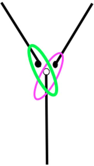
To understand the above definitions better, let us consider a simple example of a non-Hausdorff manifold. Figure 1 depicts a one-dimensional manifold that arises from gluing two ℝ¹ manifolds. Note that there is no maximal element in the bottom “trunk” of this forking structure—if it existed, it could not be mapped on an open subset of ℝ¹, so the structure would violate local Euclidicity and would not be a manifold after all. To be a manifold, each upper arm of the structure should have a minimal element. Then the pair of these elements is a witness to non-Hausdorffness: regardless of how small the neighborhoods of these pairs are, they have a nonempty intersection as they contain some part of the bottom trunk. This example (to warn the reader) is somewhat misleading, as it involves a particular bifurcating curve (defined later as a bifurcating curve of the second kind) that is hard to find in non-Hausdorff manifolds inspired by GR (see sec. 5). However, although the example clearly has no physical significance as a potential model for our world, there are other examples of non-Hausdorff manifolds that are closer to physical practice (although none of them is currently used as the proposed model of our world). We will turn to a consideration of these later.

Figure 1.

One-dimensional non-Hausdorff manifold.

In the above example, we have used an informal gluing technique as a way to construct non-Hausdorff d-manifolds from Hausdorff ones. Now, let us describe this technique formally. Then we will illustrate it by applying it to a real physics example: a non-Hausdorff extension of the so-called Taub space. We will later (in theorem 3) see that this technique provides a universal method of constructing non-Hausdorff d-manifolds out of Hausdorff d-manifolds by gluing the latter appropriately. We begin with these definitions:

Clearly, the definition implies that U ₂₁ is open as well.

Each U_ij has two indices: the first one is the index of a manifold of which it is a subset; the second one is the index of a manifold to which the first manifold is glued by the gluing function ϕ _ij. If we consider only two manifolds, the latter information is redundant; however, later (see definition 3) we will consider larger (even infinite) families of manifolds, and some of them can be glued to more than one manifold in different ways (on different subsets), so that in general $U_{\mathrm{ij}}\ne U_{\mathrm{ik}}$ for $j\ne k$ . Therefore, the notation with two indices in general does not involve redundancy.

A gluing function can be illustrated by figure 1. The two manifolds are copies of ℝ¹, ${ℝ}_i^1=\left\{〈x,i〉\mid x\in {ℝ}^1\right\}$ , where $i\in \{1,2\}$ , each with a natural global atlas. Each U_i is an open lower segment of the corresponding manifold; for example, $U_i=\{〈x,i〉\mid x\in {ℝ}^1\wedge x<0\}$ . The gluing function is given by $\varphi (〈x,1〉)=〈x,2〉$ for $〈x,1〉\in U_1$ .

A notion that we need in the definition below is that of corresponding elements from the union of manifolds, $W_1\cup W_2$ , glued by a gluing function. Clearly, $x\in W_1\cup W_2$ corresponds to itself; less trivially, x, $y\in W_1\cup W_2$ correspond to each other if they are linked by the gluing function. In the definition below, where we glue together arbitrarily many manifolds (using many gluing functions), we appeal to this notion of correspondence, requiring it to be an equivalence relation.

Clause 1 says that for any pair of d-manifolds, 〈W _μ, A _μ, g_u〉 and 〈W_v, A_v, g_v〉, there are subsets $U_{\mu \nu }\subseteq W_{\mu }$ and $U_{\nu \mu }\subseteq W_{\nu }$ that are identified by a gluing function. Clause 2 defines relation R(x, y) and postulates it to be an equivalence relation on ${\cup }_{\mu \in \Gamma }{W}_{\mu }$ . We may require instead that (i) for each map ϕ _μv there is a map ${\varphi }_{\nu \mu }={\varphi }_{\mu \nu }^{\mathrm{-1}}$ and (ii) for any two maps ${\varphi }_{\mu \nu }:U_{\mu \nu }\to U_{\nu \mu },{\varphi }_{\nu \eta }:U_{\nu \eta }\to U_{\eta \nu }$ , if $U_{\nu \mu }\cap U_{\nu \eta }\ne \varnothing$ , then there is a third map ${\varphi }_{\mu \eta }:U_{\mu \eta }\to U_{\eta \mu }$ , with $U_{\mu \eta }={\varphi }_{\nu \mu }[U_{\nu \mu }\cap U_{\nu \eta }]\subseteq U_{\mu \nu }$ and $U_{\eta \mu }={\varphi }_{\nu \eta }[U_{\nu \mu }\cap U_{\nu \eta }]\subseteq U_{\eta \nu }$ , such that for any $x\in U_{\mu \eta }$ : ${\varphi }_{\nu \eta }\left({\varphi }_{\mu \nu }\right(x\left)\right)={\varphi }_{\mu \eta }\left(x\right)$ .

Thus, clause 2 can be understood as stating a consistency condition on a family of maps, their domains, and counterdomains. Clause 3 requires one to produce a set of representatives of the quotient structure. This move might look superfluous, but it is needed later in theorem 3, in which we prove that by gluing the maximal Hausdorff submanifolds of a given manifold one obtains exactly the initial manifold, not a structurally identical manifold with points replaced by sets of points. Observe here that if a point x belongs to ${\cup }_{\mu \in \Gamma }\left(W_{\mu }\setminus {\cup }_{\eta \in \Gamma }{U}_{\mu \eta }\right)$ , it gives rise to the singleton of x, {x}, in the quotient structure, so taking a representative is trivial. Yet, a class in the quotient structure can be infinite, so one may need the axiom of choice to secure a representative of that class in clause 3. In clause 4, ${\tilde{W}}_{\mu }$ consists of counterparts of elements of W _μ in W, and f _μ is then a bijection between ${\tilde{W}}_{\mu }$ and W _μ. As for clause 5, even if p is associated with many q’s from different W _μ’s, since such q’s are connected by the isometry, the metric at all these points is the same, and hence the definition of g is consistent.

Observe that definition 3 does not require any specific relation between atlas A and atlases A _μ (in particular, we do not define A in terms of A _μ), apart from the relation between the topologies that these atlases induce (which is the topic of clause 4). This reflects the role the atlases play: they induce topologies and produce a differential structure, but for the physical content of the model it is irrelevant what specific functions these charts contain.

Before we proceed, we prove two facts that are pertinent to the definition above:

Fact 1. Let d-manifold 〈W, A_W, g〉 be a result of gluing together a family of d-manifolds ${\{〈W_{\mu },A_{W_{\mu }},g_{\mu }〉\}}_{\mu \in \Gamma }$ , with 𝒯 and 𝒯_μ ($\mu \in \Gamma$ ) being the topologies on W and W _μ, respectively. Then

(2)$\begin{array}{}& O\in 𝒯\Rightarrow {\forall }_{\mu \in \Gamma }{f}_{\mu }^{\mathrm{-1}}[O\cap {\tilde{W}}_{\mu }]\in {𝒯}_{\mu }\text{.}\end{array}$

As an immediate consequence of this fact and equation (1), we have the following fact:

At this junction we know what it means that a generalized d-manifold results from gluing together a family of Hausdorff differential d-manifolds. We do not know yet, however, whether there are instances of this definition, that is, whether there is a generalized d-manifold and a family of Hausdorff d-manifolds that are related in the way the definition above prescribes. We argue now that definition 3 has instances by proving first that the product of the gluing construction is a generalized C ⁰ manifold, that is, a generalized topological manifold.

Observe that with the above theorem we arrived at a C ⁰ n-dim non-Hausdorff d-manifold, that is, an n-dim non-Hausdorff topological manifold. To obtain a C^r ($r>0$ ) d-manifold, with its atlas resulting from atlases of component manifolds, compositions $\psi \circ f_{\eta }^{\mathrm{-1}}{({\varphi }^{\prime }\circ f_{\mu }^{\mathrm{-1}})}^{\mathrm{-1}}$ should be C^r continuous, but they do not need to be so if $\mu \ne \eta$ .Footnote ⁵ This means that to produce a C^r ($r>0$ ) d-manifold, an additional job is needed that consists in appropriately smoothing the maps ϕ and ϕ′ that belong to charts from different atlases. There are limitations to this procedure, as there are topological manifolds that do not admit a C^r ($r>0$ ) structure, as was proved by Kervaire (Reference Kervaire1960). However, it is not clear whether such troublesome topological manifolds can be constructed by our gluing procedure, which operates on a C^r d-manifold. In any case, barring Kervaire’s cases, the introduction of the required differentiability structure is possible, which suffices to ensure that our definition 3 is not empty. Besides, the problem with C^r continuity will not arise in our main theorem about the construction of non-Hausdorff d-manifolds from families of Hausdorff d-manifolds, as it selects particular families of Hausdorff d-manifolds.

3. Gluing in Action

One may wonder in what contexts non-Hausdorff d-manifolds appear in GR literature and whether such manifolds are constructible by the gluing technique. A typical context for the occurrence of a non-Hausdorff d-manifold is a failure of the well posedness of the initial value problem: if Einstein’s field equations (EFE) admit multiple solutions, these solutions can be glued together, the results being a non-Hausdorff d-manifold with a metric that still satisfies EFE. In this spirit Hawking and Ellis (Reference Hawking and Ellis1973) sketched the construction of non-Hausdorff d-manifolds that are extensions of Misner space-time and the Taub space-time. As it is far from clear that these constructions are equivalent to our gluing technique, we now describe a non-Hausdorff d-manifold obtained by gluing together extensions of the Taub space-time. An analogous technique can be used to produce more realistic general-relativistic examples, like pasting together extensions of Gowdy polarized space-time (see, e.g., Chruściel and Isenberg Reference Chruściel and Isenberg1993).

The Taub space-time is given by set $M=(t_{-},t_{+})\times S^3$ , with t ₋, $t_{+}\in \Re$ and $t_{-}<t_{+}$ . The metric is as follows:

$g=-U^{\mathrm{-1}}{\mathrm{dt}}^2+{\left(2l\right)}^{2}U{(d\psi +\cos \Theta d\varphi )}^2+(t^2+l^2)(d{\Theta }^2+{\sin }^2\Theta d{\varphi }^2)\text{,}$

where

$U\left(t\right)=\frac{(t_{+}-t)(t_{-}-t)}{t^2+l^2}\text{ and }{t}_{\pm }=m\pm {(l^2+m^2)}^{1/2}\text{,}$

m and l are positive constants, and Θ, ψ, and ϕ are Euler angles on S ³. We denote the Taub space-time by 〈M, A, g〉, where A is a maximal atlas on M. The space-time is singular at t _±, but, as first shown by Newman, Tamburino, and Unti (Reference Newman, Tamburino and Unti1963), it can be extended forward into two space-times 〈M ^↑+, A ^↑+, g ^↑+〉 and 〈M ^↑−, A ^↑−, g ^↑− 〉, each with topology $(t_{-},\infty )\times S^3$ , embeddings ${\Lambda }^{\uparrow \pm }:M\to M^{\uparrow \pm }$ , and metrics

$g^{\uparrow \pm }=\pm \left(4l\right)(d\psi +\cos \Theta d\varphi )\mathrm{dt}+{\left(2l\right)}^{2}U{(d\psi +\cos \Theta d\varphi )}^2+(t^2+l^2)(d{\Theta }^2+{\sin }^2\Theta d{\varphi }^2)\text{.}$

(To recall, to say that $\Lambda :M\to M^{\prime }$ is an embedding means that $\Lambda :M\to \Lambda \left[M\right]$ is a diffeomorphism and Λ[M] is open in the topology on M′. For details of the construction, consult Chruściel and Isenberg [Reference Chruściel and Isenberg1993].) Analogously, 〈M, A, g〉 can be extended downward into two space-times 〈M ^↓+, A ^↓+, g ^↓+〉 and 〈M ^↓−, A ^↓−, g ^↓−〉, each with topology $(-\infty ,t_{+},)\times S^3$ , embeddings ${\Lambda }^{\downarrow \pm }:M\to M^{\downarrow \pm }$ , and metrics $g^{\downarrow \pm }=g^{\uparrow \pm }$ . Importantly, the upward and downward extensions can be pair-wise pasted together, producing four space-times, known as Taub-NUT space-times: 〈M ^↑+↓+, A ⁺⁺, g ⁺⁺〉, 〈M ^↑+↓−, A ⁺⁻, g ⁺⁻〉, 〈M ^↑−↓+, A ⁻⁺, g ⁻⁺〉, and 〈M ^↑−↓−, A ⁻⁻, g ⁻⁻〉, each with topology $(-\infty ,\infty )\times S^3$ . The corresponding embeddings are denoted by $i^{\uparrow \mathrm{ab}}:M^{\uparrow a}\to M^{\uparrow a\downarrow b}$ and $i^{\downarrow \mathrm{ab}}:M^{\downarrow b}\to M^{\uparrow a\downarrow b}$ . Each Taub-NUT space-time is Hausdorff. As for isometry, Chruściel and Isenberg (Reference Chruściel and Isenberg1993) proved that while the pairs 〈M ^↑+↓+, A ⁺⁺, g ⁺⁺〉, 〈M ^↑−↓−, A ⁻⁻, g ⁻⁻〉 and 〈M ^↑+↓−, A ⁺⁻, g ⁺⁻〉, 〈M ^↑−↓+, A ⁻⁺, g ⁻⁺〉 are isometric, the pair 〈M ^↑+↓−, A ⁺⁻, g ⁺⁻〉, 〈M ^↑+↓+, A ⁺⁺, g ⁺⁺〉 is nonisometric. Note that the nonisometric pair is produced by embeddings:

$i^{\uparrow ++}:M^{\uparrow +}\to M^{\uparrow +\downarrow +}{i}^{\uparrow +-}:M^{\uparrow +}\to M^{\uparrow +\downarrow -}\text{.}$

These embeddings establish an isometry between $i^{\downarrow ++}\left[M^{\uparrow +}\right]\subseteq M^{\uparrow +\downarrow +}$ and $i^{\downarrow +-}\left[M^{\uparrow +}\right]\subseteq M^{\uparrow +\downarrow -}$ . Thus, i ^↓++[M ^↑+] and i ^↓+−[M ^↑+] establish isometric segments of otherwise nonisometric Taub-NUT space-times. Moreover, these are maximal isometric segments (Chruściel and Isenberg Reference Chruściel and Isenberg1993). We will use this fact to produce a non-Hausdorff d-manifold by means of the gluing procedure described in definition 3.

Consider nonisometric Taub-NUT space-times 〈M ^↑+↓−, A ⁺⁺, g ⁺⁻〉 and 〈M ^↑+↓+, A ⁺⁺, g ⁺⁺〉. By the definition of embedding, $U^{++}≔i^{\downarrow ++}\left[M^{\uparrow +}\right]\subseteq M^{\uparrow +\downarrow +}$ and $U^{+-}≔i^{\downarrow +-}\left[M^{\uparrow +}\right]\subseteq M^{\uparrow +\downarrow -}$ are open. Clearly, the function $i^{\downarrow +-}\circ {\left(i^{\downarrow ++}\right)}^{\mathrm{-1}}:i^{\downarrow ++}\left[M^{\uparrow +}\right]\to i^{\downarrow +-}\left[M^{\uparrow +}\right]$ and its inverse are isometries. Thus, we have two gluing functions that link the two nonisometric space-times: ${\varphi }_{12}≔i^{\downarrow +-}\circ {\left(i^{\downarrow ++}\right)}^{\mathrm{-1}}$ and ${\varphi }_{21}={\varphi }_{12}^{\mathrm{-1}}$ .

We describe now the d-manifold 〈W, A, g〉 that is a result of gluing two d-manifolds 〈M ^↑+↓−, A ⁺⁻, g ⁺⁻〉 and 〈M ^↑+↓+, A ⁺⁺, g ⁺⁺〉 in accord with definition 3. The glued subsets are $U^{++}\subseteq M^{\uparrow +\uparrow +}$ and $U^{+-}\subseteq M^{\uparrow +\downarrow -}$ , the gluing functions being ϕ ₁₂ and ϕ ₂₁. As we have only these two gluing functions, it is easy to see that R(x, y) is indeed an equivalence relation on the union $M^{\uparrow +\downarrow +}\cup M^{\uparrow +\downarrow -}$ . We thus take for W a set of representatives of $(M^{\uparrow +\downarrow +}\cup M^{\uparrow +\downarrow -})/R$ . Next we define the topology on W as the coarsest-grained topology that satisfies $O\in {𝒯}^{++}\to f_{++}\left[O\right]\in 𝒯$ and $O\in {𝒯}^{+-}\to f_{+-}\left[O\right]\in 𝒯$ , where 𝒯^+± is the topology induced by atlas A ^+± on M ^↑+↓±. We chose a maximal atlas on W that yields exactly this topology. Finally, to unpack clause 5, the metric g(p), $p\in W$ and metrics g ⁺⁺(q), $q\in M^{++}$ (or g ⁺⁻(q), $q\in M^{+-}$ ) agree whenever p and q belong to same equivalence class. However, this occurs if p and q are identical or linked by a gluing function (which is an isometry), so the clause is indeed satisfied.

We now claim that the d-manifold 〈W, A, g〉, constructed as above, is non-Hausdorff.

We arrived thus at a non-Hausdorff manifold that resulted from gluing together nonisometric Taub-NUT space-times. The introduction of such objects to GR was motivated by a desire to have solutions to EFE that are as large as possible, but there are trade-offs in this chase for even larger solutions. The topologically nice (globally hyperbolic and Hausdorff) but small Taub space-time yields to larger Taub-NUT extensions (not globally hyperbolic but still Hausdorff), which in turn yield to non-Hausdorff manifolds resulting from gluing together the former extensions. The first two kinds of object are typically classified as GR space-times. Is the third object a GR space-time as well? If not, how should one understand it? Before we address these questions, in the next section we put forward two theorems that, we believe, suggest and support a modal interpretation of non-Hausdorff manifolds in GR.

4. Hausdorff versus Non-Hausdorff Manifolds

In this section we prove that any non-Hausdorff d-manifold occurring in GR can be seen as a result of pasting together a family of Hausdorff d-manifolds.Footnote ⁶ We give first an auxiliary theorem that any non-Hausdorff manifold can be decomposed into maximal Hausdorff submanifolds.Footnote ⁷

We have finally come to the main theorem of this article:

The theorem provides an underpinning for the modal interpretation of a non-Hausdorff manifold occurring in GR, which sees it as encapsulating a bundle of alternative GR space-times, all of which are compatible with the initial data set. Their support for the modal interpretation comes from the universality the theorems bring. Just think of a non-Hausdorff manifold produced in the context of a failure of the initial value problem. The theorems then say that this manifold can be decomposed into maximal Hausdorff submanifolds and the decomposition is faithful in the sense that the initial non-Hausdorff manifold is recovered by gluing these submanifolds together. Moreover, whenever gluing identifies some regions of submanifolds, these regions are physically alike (they are identical). A non-Hausdorff manifold, whose maximal Hausdorff submanifolds have some additional features so they qualify as GR space-times, naturally reads as a bundle of GR space-times that is glued together in physically identical regions. Further, if the metrics on the submanifolds satisfy EFE, the submanifolds are arguably physically possible and are compatible with the physical situation in regions of overlap.

There is one caveat concerning the universality of modal interpretation. The gluing procedure can glue together regions that are in any possible relation to a specified region: they can be to the past or to the future of it or related to it in a space-like way. Here emerges an interesting question of whether one can glue two manifolds in a fully atemporal way, that is, such that for any point in the glued-together region, the region has alternative developments only in the space-like directions. It would be difficult to treat such cases as instances of indeterminism, because the latter amounts to the existence of alternative future temporal developments. However, we do not know whether constructions of this type are possible.

One might wonder how our talk of the modal interpretation of non-Hausdorff manifolds relates to the large landscape of positions in modal metaphysics. Although our construction is conceptually modest, and hence does not provide the means to give any definite answers to this question, its features make the concept better aligned with some of the positions in modal metaphysics than others. The vision underlying a generalized manifold is that of the totality of physically possible events (idealized to be point-like) that can evolve to occur from some initial state of our universe. This totality forms a base set of a generalized manifold. Some events from this set can occur together—in the jargon of the metaphysician, they are compatible. Some other events cannot occur together; they are incompatible. Compatibilities and incompatibles are induced by events belonging to space-times: if there is a space-time to which two events belong, they are compatible; otherwise, they are incompatible. This idea naturally extends to the compatibility (incompatibility) of arbitrarily large sets of events.

The notion of space-time is in turn defined by a topological criterion: a space-time is a maximal Hausdorff submanifold of a given generalized manifold. Clearly, if a considered generalized manifold is Hausdorff, it has a single space-time, which is identical to the manifold in question. One division in modal metaphysics is between possible worlds (David Lewis) and possible ways of one (actual) world (Saul Kripke, Robert Stalnaker). Are we thus to represent alternative possibilities in terms of a multiplicity of worlds, or rather a multiplicity of maximal alternative states available for our (one) world? We opt for the latter: we think of a given generalized manifold as encapsulating modal and nonmodal features of our world; alternative space-times are like alternative maximal states available to the world. The daunting question then is which of these maximal states (space-times) is actual or is being made actual? A generalized manifold does not tell us which of these possibilities is actual, or will become actual, however. It merely encapsulates alternative possibilities (if it is non-Hausdorff). The information as to which alternative possibility is actual must come from the outside.Footnote ⁹ Yet, given the multiplicity of states, it is precisely one of these possible states that is actual or is gradually becoming actual. Emphatically, there is no answer to the question of why this possibility rather than some other is actualized. After all, we assume nonepistemic indeterminism. We thus advise the reader to reconcile with the idea that there might be no answer as why a particular space-time, out of many alternative space-times, is actualized.

Fearing that these remarks merely open up more questions than they answer, we leave the task of relating modally interpreted generalized manifolds to positions in modal metaphysics as a project for the future.

5. Bifurcating Curves—Friends or Foes?

There is a staple objection against non-Hausdorff manifolds that (1) they admit bifurcating curves or bifurcating geodesics and that (2) such bifurcating objects are bad. Against 2 we argue that on the modal interpretation of non-Hausdorff manifolds, such bifurcating objects are not bad; to the contrary, they are very much welcome. However (we continue to argue), there is typically no room for bifurcating geodesics in non-Hausdorff manifolds, in contrast to objection 1. As we would like to have bifurcating geodesics, we are not happy about the second argument.

To give some examples of the objection to bifurcating geodesics, since a geodesic is standardly assumed to be a (potential) world line of a free test particle, Earman (Reference Earman and Dieks2008, 200) asked “how would such a particle know which branch of a bifurcating geodesic to follow?” In a similar vein, Hawking and Ellis (Reference Hawking and Ellis1973, 174) opined that “a [bifurcating] behavior of an observer’s world-line would be very uncomfortable,” with “one branch going into one region and another branch going into another region.” Hájíček (Reference Hájíček1971b, 79) observed that a system cannot have two solutions unless these solutions form a bifurcating curve and concludes: “Therefore, in view of the classical causality conception coinciding with determinism it is sensible to rule out the bifurcate curves.”

These objections seem to simply beg the question in favor of determinism. It is perfectly conceivable that there is no answer as to why one possible evolution actually occurs rather than another. Whether there is always such an answer is to be settled by the physical reality and not by our methodological assumptions. Similarly, an indeterministically evolving observer might go into one spatiotemporal region or another. A comparison with the mainstream thinking (i.e., barring some hidden-variable theories) on quantum phenomena might help. We do not expect that there must be an answer to the question of “why did an electron go one way rather than the other in the Stern-Gerlach apparatus?”

To relate these observations to objection 2, an intuitive way of picturing indeterminism conceives of it as being produced locally in space and time. That is, if we contemplate alternative evolutions, musing, for instance, why one rather than the other has actualized, we wonder when and where one of these evolutions stopped being possible and what brought this about. Arguably, in such contexts we are after a well-localized object. A paradigmatic example is a pointer to a well-localized electron in a Stern-Gerlach device: before it enters the device, scenarios with traces at the bottom or top of the photographic plate are possible, but after the electron has left the device only one of them is possible. The behavior of the electron in the Stern-Gerlach device is seen as underlying the dynamics of the global scenarios: once two alternative scenarios were possible, but later only one was possible. Clearly, a similar appeal to the behavior of well-localized objects to explain the dynamics of global scenarios is even more dominant in human affairs, when the fact that we live in one scenario rather than another is attributed to agents’ choices. We call this variety of indeterminism “local indeterminism.”

On local indeterminism, alternative evolutions of a big system (our world included) require alternative evolutions of at least one of its small components. As one idealizes the component to be point-like, the alternative evolutions can be seen as alternative trajectories with two coinciding segments and two separate segments. With further assumptions, such trajectories can be represented as functions from a real interval to a manifold’s base set. Needless to say, trajectories representing alternative evolutions bifurcate. As the standard view on geodesics identifies them with trajectories of (test) particles, it follows that geodesics representing alternative evolutions of a (test) particle bifurcate as well. Accordingly, if cases of nonunique solutions to EFE mean indeterminism, and the indeterminism in question is local, there must be bifurcating curves.

Turning to objection 1, a pertinent question is whether non-Hausdorff manifolds indeed imply the existence of bifurcating curves. There is a compelling intuition linking non-Hausdorffness to bifurcating curves, to be seen in figure 1. This intuition works like this: suppose we have a pair of points, e ₁ and e ₂, witnessing a failure of the Hausdorff condition. Then it ‘must’ be possible to draw two continuous lines, one passing through e ₁ and the other passing through e ₂ in such a way that they coincide below the two points but do not overlap above them, where ‘below’ and ‘above’ are purely conventional. Thus, the picture suggests that we can always use a failure of Hausdorffness to produce bifurcating curves. This issue is more subtle, however, as the answer is different for two different types of curves: those having a maximal element in their shared part and those that instead have minimal elements in their separate arms. It turns out that the latter are not admitted by some non-Hausdorff manifolds. For an analysis of how it is possible in a physically relevant case of a non-Hausdorff extension of Misner space-time, see Margalef-Bentabol and Villaseñor (Reference Margalef-Bentabol and Villaseñor2014). (This case is relevant, as the extension is produced by the pasting technique of definition 3.) Under what conditions non-Hausdorff d-manifolds admit bifurcating curves is thus a nontrivial question that is answered by Hájíček’s (Reference Hájíček1971a) theorem, stated below.

After this preview, let us do some work. First (to recall), by a curve one means a continuous function from a real interval to a manifold’s base set, and a geodesic is a curve that satisfies the geodesic equation. Does uniqueness obtain for geodesics, and if so, is Hausdorffness needed for uniqueness to obtain? Beginning with local uniqueness, in a Hausdorff or non-Hausdorff d-manifold alike, if a metric g is appropriately continuous, given a point p and a vector at this point, in some neighborhood of p there is a unique geodesic that passes through the point and whose tangent at this point coincides with the vector.Footnote ¹⁰ Hausdorffness permits strengthening this local result to global uniqueness: for a Hausdorff d-manifold M, given the continuity condition on g, a point $p\in M$ and a vector ξ at p, there is a unique maximal geodesic $\gamma :I\to M$ such that (1) $\gamma \left(0\right)=p$ and (2) $\dot{\gamma }\left(0\right)=\xi$ , where $\dot{\gamma }\left(0\right)$ stands for a tangent to γ at point $p=\gamma \left(0\right)$ . The maximality of γ means that if there is some other geodesic ${\gamma }^{\prime }:I^{\prime }\to M$ satisfying conditions analogous to 1 and 2 above, then $I^{\prime }\subseteq I$ . In sum (given the continuity assumption on g), no geodesics can bifurcate in Hausdorff manifolds, but non-Hausdorff manifolds might be conductive to bifurcating geodesics.

Having the distinction between global and local uniqueness of geodesics, we link it to two kinds of bifurcation (e.g., Hájíček Reference Hájíček1971a).

Thus, in a bifurcating curve of the first kind, there is a maximal element of interval I at which C ₁ and C ₂ agree, whereas in a bifurcating curve of the second kind there is no maximal element in I at which C ₁ and C ₂ agree.

Now, as in a generalized d-manifold a geodesic is uniquely determined, locally speaking, by a point and a vector, no geodesics can make a bifurcating curve of the first kind. Thus, there is no room for bifurcating geodesics of the first kind in generalized d-manifolds. But local uniqueness alone does not preclude bifurcating curves of the second kind. Such curves are precluded by global uniqueness, and global uniqueness is true in Hausdorff d-manifolds. Thus, if there are bifurcating geodesics, they are of the second kind and in a non-Hausdorff manifold. But are they there?

As we have shown, any non-Hausdorff d-manifold is constructible from a family of Hausdorff manifolds, so perhaps this information can shed light on the existence of bifurcating curves (of the second kind) in these manifolds? As we will see, this is indeed the case.

We need an auxiliary notion to begin with.

As every non-Hausdorff d-manifold is constructible by gluing Hausdorff d-manifolds, Hájíček’s theorem yields a universal method to decide whether it admits bifurcating geodesics.

We use theorem 4 to argue that ‘sound’ non-Hausdorff d-manifolds (to be explained soon) occurring in GR are not continuously extendible and, hence, do not admit bifurcating curves of the second kind. Let us return to our GR example: the construction of the non-Hausdorff extension of the two Taub-NUT space-times exhibited in section 3. The open sets U ⁺⁺ and U⁺⁻, glued together by isometry ϕ ₁₂, are maximal isometric subsets of M ^↑+↑+ and M ^↑+↓−, respectively. Thus, any function $f:M^{\uparrow +\uparrow +}\to M^{\uparrow +\downarrow -}$ that properly extends ϕ ₁₂ is not an isometry, so it is not a gluing function. Accordingly, the gluing that produces a non-Hausdorff extension of the Taub space-time is not continuously extendible. Ergo, the non-Hausdorff extension of the Taub space-time admits no bifurcating curves of the second kind.

From a mathematical perspective, there are non-Hausdorff d-manifolds produced by a continuously extendible gluing procedures as well as non-Hausdorff d-manifolds produced by a noncontinuously extendible gluing procedures. The former admit bifurcating curves of the second kind, whereas the latter do not. As we have just seen, the non-Hausdorff extension of the Taub space-time belongs to the latter kind—it admits no bifurcating curves of the second kind. What about the others? We will argue that all non-Hausdorff manifolds of the former type are in a certain sense unnatural, especially when viewed from the perspective of the modal interpretation developed in this article.

Observe that the crucial move of the above argument is that the regions identified by the gluing function are maximal isometric regions of the component manifolds. A corresponding requirement is not part of definition 3 of the gluing function and is not part of definition 3 of the gluing procedure. These definitions describe an abstract mathematical object, a generalized d-manifold, and its relation to Hausdorff manifolds, understood as its components. They do not pay attention to how and at which end the defined procedure can be applied.

The application we investigate and advertise aims to produce a modal representation of a spatiotemporal world: if there are nonunique solutions of EFE for some data (which, by the Choquet-Bruhat and Geroch [Reference Choquet-Bruhat and Geroch1969] theorem, cannot be globally hyperbolic), we consider these solutions as alternative possible evolutions that start from an initial data set, and we paste them together into a non-Hausdorff manifold. In this application a natural directive is to identify (by gluing) whatever can be identified, following the idea that indeterminism requires a qualitative difference between alternative possible scenarios. This amounts to the requirement to glue together maximal isometric regions of component manifolds if there are such regions. Gluing larger regions is excluded by definitions 2 and 3, but gluing smaller than maximal isometric regions is allowed by these definitions.

To accommodate the desideratum to glue together maximal isometric regions of component manifolds, one may add this postulate to definition 3:

The left-hand side means that two points, each from a different component manifold, give rise to one and the same point in the non-Hausdorff d-manifold, whereas the right-hand side says that the points belong to appropriate isometric open subsets and are linked by a corresponding isometry.

Clearly, postulate 1 raises mathematical or interpretational issues: Do any two Hausdorff d-manifolds admit maximal isometric regions? Even if in a collection of Hausdorff d-manifolds any two of them have maximal isometric regions, does the gluing procedure always satisfy postulate 1 (i.e., does the multiplicity of components get in the way?)? Can there be nonconnected maximal isometric regions, and if so, how are we to interpret the resulting non-Hausdorff manifold?

We leave these issues aside, as they are somewhat tangential to the main observation of this section. This observation is, in a nutshell, that the more successful one is in delivering a modal representation of multiple solutions to EFE, the less likely are the bifurcating curves of the second kind. We take it that a successful representation of indeterminism calls for the satisfaction of postulate 1. This postulate requires gluing functions to identify maximal isometric regions, which means that the functions are not continuously extendible, so, by theorem 4 the resulting non-Hausdorff manifold does not admit bifurcating curves of the second kind and, hence, does not admit bifurcating geodesics of the second kind. Since, to recall, by the geodesic equation there are no bifurcating geodesics of the first kind either, there are no bifurcating geodesics. But, it might happen that a particular set of multiple solutions to EFE does not satisfy the postulate, in which case the modal interpretation of these solutions is doubtful. Yet a failure of the postulate may open the door for bifurcating curves (geodesics) of the second kind.

We find this situation deeply paradoxical. In a nutshell, given a set of multiple solutions to EFE, the better the case it makes for the indeterminism of GR, the worse it is for local indeterminism. Perhaps a way out is to countenance a nonlocal variety of indeterminism. This comes with a price, however, as the divergence of the two notions of local and global indeterminism is deemed counterintuitive (see, e.g., Belot Reference Belot1995; Melia Reference Melia1999; Sattig Reference Sattig2015).

6. Conclusion

Our article revolves around two questions, both related to non-Hausdorff manifolds in GR: (1) What can these manifolds represent? And, in particular, (2) can they be used to represent indeterminism, modally understood? The main formal result in the light of which we studied these questions says that every non-Hausdorff d-manifold can be constructed by gluing together a family of Hausdorff d-manifolds. This of course means that the gluing procedure delivers every non-Hausdorff d-manifold of GR as well. Typically, the construction of these manifolds in GR is motivated by the desire to produce a possibly large solution of EFE, and gluing together nonisomorphic solutions to EFE is a way to achieve this goal. The side effect of this procedure, however, is that the resulting objects are non-Hausdorff. Since Hausdorffness is standardly required for a manifold to represent a GR space-time, the question emerges of what such non-Hausdorff manifolds constructed in GR can represent.

Our response to this question is twofold: we conservatively keep the requirement of Hausdorffness for GR space-times, while viewing a non-Hausdorff manifold produced by gluing together a set of nonunique solutions to EFE as a modal representation of this set. That is, we read such a manifold as encapsulating multiple possible spatiotemporal evolutions (space-times), every one of which is compatible with a given initial data set; this looks like a clear case of indeterminism. We concede that non-Hausdorff manifolds produced outside of the context of the initial value problem might have no interpretation.

To adopt this interpretation, we argued that a non-Hausdorff manifold should be constructible by a more stringent gluing procedure, one that satisfies postulate 1 as well. Although a non-Hausdorff manifold whose components are nonisometric Taub-NUT space-times is constructible by the more stringent procedure, we do not know whether this more stringent gluing procedure can be performed for all cases. More worryingly (from a philosophical perspective), postulate 1 has a consequence (via theorem 4) that spells trouble for the modal interpretation: there are no bifurcating curves and, hence, no bifurcating geodesics in a non-Hausdorff manifold obtained by the gluing procedure that satisfies the postulate.

As we argued, the usual notion of indeterminism is local: if there are alternative evolutions of a big system, some small component of this system has to have alternative trajectories. Since geodesics are standardly identified with trajectories of free (test) particles, the fact that there are no bifurcating geodesics excludes local indeterminism. Thus, a non-Hausdorff manifold produced in accord with postulate 1 cannot represent locally indeterministic evolutions. It looks like we are thus back to square one: What can non-Hausdorff manifolds represent?

The answer depends on what stance one takes to a nonlocal variety of indeterminism, which might, and in GR cases does, conflict with the local variety. If we accept the nonlocal notion, there is no obstacle to reading a non-Hausdorff manifold produced from nonunique solutions of EFE in accord with postulate 1 as the representation of nonlocal indeterminism. After all, relativistic physics has questioned a few intuitive notions, so its verdict that there might be indeterminism without local indeterminism should not come as a big shock. But, arguing in the opposite direction, one might recall that GR is concerned with big rather than small objects, so its failure to accommodate local indeterminism might just reflect its neglect of micro objects. Another option is to consider non-Hausdorff manifolds as they occur in GR contexts as purely mathematical objects without any physical meaning. Finally, the old option of some physicists—allowing for non-Hausdorff space-times—might be back on the table: their main objection to non-Hausdorffness was that it introduces bifurcating geodesics, but as we saw, there are no such geodesics if postulate 1 is accommodated.Footnote ¹¹

We leave to the reader the choice as to which option is preferred.