
1. Introduction
Large-eddy simulation (LES) has achieved great success in the numerical investigation of turbulent flows, and it has already been widely used in studying the mechanism of turbulence and in simulating practical engineering flows (Larchevêque et al. Reference Larchevêque, Sagaut, Lê and Comte2004; Fureby Reference Fureby2008). The most widely used subgrid-scale (SGS) model is the eddy-viscosity model (Lesieur & Métais Reference Lesieur and Métais1996), and the first SGS eddy-viscosity model was the Smagorinsky model (Smagorinsky Reference Smagorinsky1963; Deardorff Reference Deardorff1970). Using the eddy-damped quasi-normal Markovian theory, Chollet & Lesieur (Reference Chollet and Lesieur1981) suggested the spectral eddy-viscosity model, which is suitable for homogeneous and isotropic turbulence. Based on the square of the velocity gradient tensor, Nicoud & Ducros (Reference Nicoud and Ducros1999) proposed a wall-adapting local eddy-viscosity model (WALE), which can well simulate wall-bounded flows without a dynamic procedure. The Vreman (Reference Vreman2004) model is another SGS eddy-viscosity model suitable for the LES of turbulent shear flows. Yu et al. (Reference Yu, Hong, Xiao and Chen2013) presented a new form of SGS viscosity according to SGS helicity dissipation balance and a spectral relative helicity relation in the inertial subrange of helical turbulence, and this model can simulate shear and separated turbulent flows with satisfactory results. Recently, Pickering et al. (Reference Pickering, Rigas, Schmidt, Sipp and Colonius2021) proposed a data-informed method to test which eddy-viscosity model could improve the alignment between observed large-scale structures and those computed from resolvent analysis. Leoni et al. (Reference Leoni, Zaki, Karniadakis and Meneveau2021) developed a new eddy-viscosity model based on fractional gradients, and it could accurately predict the non-local behaviour of subfilter stress–strain-rate correlation functions. In addition to the eddy-viscosity model, the structural model is an important type of SGS model, which provides a high correlation with the real SGS stress (Meneveau & Katz Reference Meneveau and Katz2000). One of the structural models is the gradient model, which was originally proposed by Clark, Ferziger & Reynolds (Reference Clark, Ferziger and Reynolds1979) and then was developed by Vreman, Geurts & Kuerten (Reference Vreman, Geurts and Kuerten1996). The gradient model can be derived from the Taylor expansion of the filtered velocity for the SGS stress. The scale-similarity model (SSM) is another structural model, which is based on the scale-similarity hypothesis (Bardina, Ferziger & Reynolds Reference Bardina, Ferziger and Reynolds1980; Liu, Meneveau & Katz Reference Liu, Meneveau and Katz1994). According to the assumption of scale invariance, the SSM is developed in a similar form as an SGS stress tensor of a larger-scale flow field using the resolved velocity, and the SSM also has a high correlation with the real SGS stress.
The famous dynamic procedure was proposed by Germano et al. (Reference Germano, Piomelli, Moin and Cabot1991), using the Germano identity to dynamically determine the coefficient of the SGS model in the LES of turbulent flows. Subsequently, Lilly (Reference Lilly1992), Piomelli (Reference Piomelli1993), Ghosal et al. (Reference Ghosal, Lund, Moin and Akselvoll1995) and Meneveau, Lund & Cabot (Reference Meneveau, Lund and Cabot1996) improved and generalized the dynamic procedure. With the Germano identity, Yu, Xiao & Li (Reference Yu, Xiao and Li2016) derived an expression for the energy flux at the test-filter scale, which can be adopted to optimize the coefficients of SGS models. Incorporating physical constraints into the SGS model can also improve the reliability and accuracy of the model. Chen et al. (Reference Chen, Xia, Pei, Wang, Yang, Xiao and Shi2012) introduced Reynolds stress to constrain the SGS model in the inner layer of wall-bounded turbulent flows to make the prediction of mean velocity, turbulent stress and skin-friction coefficient more accurate, which is called the Reynolds-stress-constrained LES.
Nevertheless, the traditional LES requires further improvements in transitional flows (Sayadi & Moin Reference Sayadi and Moin2012), compressible flows (Piomelli Reference Piomelli1999) and low-Reynolds-number regions (Voke Reference Voke1996; Meneveau & Katz Reference Meneveau and Katz2000). Horiuti (Reference Horiuti1986) employed the standard Smagorinsky model (SM) to simulate the transitional channel flow and found that this model cannot properly predict the transition process due to excessive dissipation. Huai, Joslin & Piomelli (Reference Huai, Joslin and Piomelli1997) applied the dynamic Smagorinsky model (DSM) to the simulation of a transitional flat-plate boundary layer for the first time and obtained acceptable results. Sayadi & Moin (Reference Sayadi and Moin2012) evaluated several commonly used SGS models in LES of transitional flows. They found that the dynamic procedure could accurately predict the transition. Recently, Bodart & Larsson (Reference Bodart and Larsson2012) proposed a laminar/turbulent sensor to the traditional wall model and successfully predicted the transition. Moin et al. (Reference Moin, Squires, Cabot and Lee1991) suggested a compressible DSM model for the first time and applied the model to the simulation of compressible isotropic turbulence. Chai & Mahesh (Reference Chai and Mahesh2012) proposed a dynamic one-equation eddy-viscosity model for the LES of compressible flow and applied it to decaying isotropic turbulence and normal shock–isotropic turbulence interactions.
For the traditional LES, most SGS models are developed based on the scale-invariance hypothesis. Voke (Reference Voke1996) provided a fitted relation between the SGS viscosity of the SM and the mesh Reynolds number based on some theoretical models of the energy spectrum. This scale-dependent SM was an attempt to overcome the limitation of the scale-invariance hypothesis, and the simulation results were improved slightly when the cutoff was in the dissipation range. Meneveau & Lund (Reference Meneveau and Lund1997) proposed a fitting ratio of the test-scale to the grid-scale coefficient of the SM and applied the scale-dependent DSM to simulate forced isotropic turbulence. Porté-Agel, Meneveau & Parlange (Reference Porté-Agel, Meneveau and Parlange2000) generalized the scale-dependent DSM to simulate a neutral atmospheric boundary layer.
More recently, artificial neural networks (ANNs) have become an increasingly popular method for developing turbulence models (Duraisamy, Iaccarino & Xiao Reference Duraisamy, Iaccarino and Xiao2019). Ling, Kurzawski & Templeton (Reference Ling, Kurzawski and Templeton2016) adopted a new multiplicative-layer neural network with an invariant tensor to predict the Reynolds stress anisotropic tensor for the first time. Taking advantage of machine learning and optimal evaluation theory, Vollant, Balarac & Corre (Reference Vollant, Balarac and Corre2017) developed a new SGS scalar flux model. The deconvolution of turbulence variables can also be obtained through an ANN (Maulik & San Reference Maulik and San2017), and it showed excellent behaviour in an a priori test. Zhou et al. (Reference Zhou, He, Wang and Jin2019b) developed a new SGS model through the ANN method for isotropic turbulence, and it considered the dependence of the SGS model on the filter width. Xie et al. (Reference Xie, Wang, Li, Wan and Chen2019) proposed an ANN-based mixed model combining the SM and the gradient model, and the new model showed better behaviour in a priori and a posteriori tests than traditional LES models. Using neural networks trained by full turbulent channel flow data, Yang et al. (Reference Yang, Zafar, Wang and Xiao2019) discussed several problems encountered in wall modelling of LES. Using the direct numerical simulation (DNS) data of incompressible isotropic turbulence, ANN-based nonlinear algebraic models and deconvolutional models have been developed (Xie, Wang & Weinan Reference Xie, Wang and Weinan2020a; Xie, Yuan & Wang Reference Xie, Yuan and Wang2020b; Yuan, Xie & Wang Reference Yuan, Xie and Wang2020), which could clearly improve the accuracy of the model compared with the traditional SGS models and implicit large-eddy simulation (ILES).
In addition, machine learning methods have been employed for super-resolution reconstruction of turbulent flows (Maulik & San Reference Maulik and San2017; Fukami, Fukagata & Taira Reference Fukami, Fukagata and Taira2019; Kim & Lee Reference Kim and Lee2020; Liu et al. Reference Liu, Tang, Huang and Lu2020; Yuan et al. Reference Yuan, Xie and Wang2020; Kim et al. Reference Kim, Kim, Won and Lee2021). Such reconstruction can be used to improve predictions based on coarse wall measurements in wall-bounded turbulence (Güemes et al. Reference Güemes, Discetti, Ianiro, Sirmacek, Azizpour and Vinuesa2021; Vinuesa & Brunton Reference Vinuesa and Brunton2021). In past studies, some completely black-box models based on ANN methods have been developed in LES modelling of wall-bounded turbulence. Through a priori test and a posteriori test, Park & Choi (Reference Park and Choi2021) found that the SGS model is unstable with the input variables at multiple points, but stable with the input variables at a single point, and the single-point input variables will also be adopted in this study.
In this paper, we propose a kinetic-energy-, ux-constrained model (KCM) using the ANN method for the LES of compressible wall-bounded turbulence. The structure of the paper is as follows. The LES governing equations and modelling background are introduced in § 2. The theoretical deduction of the new constrained model is given in § 3, followed by the DNS of the compressible channel flow and the ANN method in § 4. In § 5, the LES results of compressible turbulent channel flow and the compressible flat-plate boundary layer are presented and analysed. Finally, the discussion and conclusions are given in § 6.
2. Theoretical background
2.1. LES governing equations
For the general applicability of the research, we derive the LES governing equations of compressible flows as follows:
 $$\begin{gather} \frac{\partial\bar{\rho}}{\partial t}+\frac{\partial \bar{\rho}\tilde{u}_j}{\partial x_j}=0, \end{gather}$$
 $$\begin{gather}\frac{\partial \bar{\rho}\tilde{u}_i}{\partial t}+\frac{\partial \bar{\rho}\tilde{u}_i\tilde{u}_j}{\partial x_j}+\frac{\partial \bar{p}}{\partial x_i}=\frac{\partial\tilde{\sigma}_{ij}}{\partial x_j}-\frac{\partial \tau_{ij}}{\partial x_j}, \end{gather}$$
 $$\begin{gather}\frac{\partial \bar{\rho}\tilde{E}}{\partial t}+\frac{\partial (\bar{\rho}\tilde{E}+\bar{p})\tilde{u}_j}{\partial x_j}={-}\frac{\partial \tilde{q}_j}{\partial x_j}+\frac{\partial\tilde{\sigma}_{ij}\tilde{u}_i}{\partial x_j}-\frac{\partial C_pQ_j}{\partial x_j}-\frac{\partial \mathcal{J}_j}{\partial x_j}, \end{gather}$$
 $$\begin{gather}\bar{p}=\bar{\rho}R\tilde{T}, \end{gather}$$
where an overbar ( $\bar {\cdot }$) denotes spatial filtering at scale
 $\varDelta$ using a smooth low-pass filter function
 $G(\boldsymbol r)$ (e.g.
 $\bar {\rho }(x)=\int G(\boldsymbol r)\rho (x+r)\, \textrm {d} \boldsymbol r$ represents the resolved density field) and a tilde (
 $\tilde {\cdot }$) denotes spatial Favre filtering as
 $\tilde {\phi }={\overline {\rho \phi }}/{\bar {\rho }}$.
In (2.1)–(2.4),  $\rho, u_i, T, E$ and
 $R$ denote the density, velocity, temperature, total energy and specific gas constant, respectively. The resolved viscous stress tensor
 $\tilde {\sigma }_{ij}$ and the heat flux vector
 $\tilde {q}_j$ are given by
 $$\begin{gather} \tilde{\sigma}_{ij}=2\mu(\tilde{T})(\tilde{S}_{ij}- \tfrac{1}{3}\delta_{ij}\tilde{S}_{kk}), \end{gather}$$
 $$\begin{gather}\tilde{q}_j=\frac{C_p \mu(\tilde{T})}{Pr}\frac{\partial\tilde{T}}{\partial x_j}, \end{gather}$$
where  $C_p$ and
 $Pr$ are the specific heat at constant pressure and the molecular Prandtl number,
 $\mu = ({1}/{{Re}}){( {{{\tilde T}}/{{{{\tilde T}_\infty }}}} )^{3/2}}[({{{{\tilde T}_\infty } + {T_s}}})/({{\tilde T + {T_s}}})]$ is the molecular viscosity calculated using Sutherland's law for a given
 $T_s=110.3~\mathrm {K}$,
 $Re=\rho _{\infty }U_{\infty }L/\mu _{\infty }$ is the Reynolds number and
 $\tilde {S}_{ij}=\frac {1}{2}({\partial \tilde {u}_i}/{\partial x_j}+{\partial \tilde {u}_j}/{\partial x_i})$ is the resolved strain-rate tensor.
In (2.1)–(2.3), there are some unclosed terms, including the SGS stress tensor
 \begin{equation} {\tau}_{ij}=\bar{\rho}(\widetilde{u_iu_j}-\tilde{u}_i\tilde{u}_j), \end{equation}
the SGS heat flux
 \begin{equation} Q_j=\bar{\rho}(\widetilde{u_jT}-\tilde{u}_j\tilde{T}) \end{equation}
and the SGS turbulent diffusion
 \begin{equation} \mathcal{J}_j=\tfrac{1}{2}(\bar{\rho}\widetilde{u_ju_iu_i}- \bar{\rho}\tilde{u}_j\widetilde{u_iu_i}). \end{equation}
It is suggested that SGS turbulent diffusion can be approximated as  $\mathcal {J}_j=\tau _{ij}\tilde {u}_i$ (Martin, Piomelli & Candler Reference Martin, Piomelli and Candler2000). The SGS stress tensor
 ${\tau }_{ij}$ and the SGS heat flux
 $Q_j$ need to be modelled based on the resolved quantities. The models for these terms are discussed below.
2.2. Subgrid-scale model
In LES, the eddy-viscosity model is the most commonly used SGS stress model for  $\tau _{ij}$, and it is a phenomenological model. The SGS stress tensor is modelled by a term with a structure similar to that of viscous stress. Using a subgrid viscosity
 $\mu _{sgs}$ to mimic the molecular viscosity, the formulation of the SGS stress
 $\tau _{ij}$ is written as
 \begin{equation} \tau^{mod}_{ij}-\tfrac{1}{3}\delta_{ij}\tau^{mod}_{kk}={-}2\mu_{sgs}(\tilde{S}_{ij}- \tfrac{1}{3}\delta_{ij}\tilde{S}_{kk}). \end{equation}
The typical expression of  $\mu _{sgs}$ in (2.10) is the SM (Smagorinsky Reference Smagorinsky1963), which is obtained from the resolved strain-rate tensor. Then,
 \begin{equation} \mu_{sgs}=\bar{\rho}C_{sm}\varDelta^2|\tilde{S}|, \end{equation}
with
 \begin{equation} |\tilde{S}|=\sqrt{2\tilde{S}_{ij}\tilde{S}_{ij}}, \end{equation}
and  $C_{sm}$ is the coefficient of the anisotropic part of the SM. The isotropic part of the SGS tensor is
 \begin{equation} \tau^{mod}_{kk}=2C_I\bar{\rho}\varDelta^2|\tilde{S}|^2, \end{equation}
and  $C_I$ is the coefficient of the isotropic part of the SM (Yoshizawa Reference Yoshizawa1986). The SGS heat flux can be modelled as
 \begin{equation} {Q}^{mod}_j={-}\frac{\mu_{sgs}}{Pr_t}\frac{\partial\tilde{T}}{\partial x_j}, \end{equation}
where  $Pr_t$ is the SGS Prandtl number.
3. Kinetic-energy-flux-constrained model (KCM)
Since the proposal of the first concept of the energy cascade by Richardson, research on the energy cascade has always been the core content of turbulence studies (Pope Reference Pope2000), and it is also the most well-known statistical characteristic in LES (Moser, Haering & Yalla Reference Moser, Haering and Yalla2021). Kolmogorov (Reference Kolmogorov1941) quantitatively formulated the energy cascade for the first time
and suggested that the kinetic energy flux (KEF) is constant in the inertial subrange of locally isotropic turbulence, where the energy flux refers to the energy transfer rate from the large scale to the small scale. Subsequently, a variety of studies have focused on the KEF of incompressible and compressible turbulent flows (Meneveau & Sreenivasan Reference Meneveau and Sreenivasan1987; Borue & Orszag Reference Borue and Orszag1998; Eyink Reference Eyink2006; Wang et al. Reference Wang, Yang, Shi, Xiao, He and Chen2013). The KEF between different-scale eddies is the essence of the energy cascade and reflects the dynamic process of the generation and evolution of turbulence. The accurate prediction of KEF at different scales guarantees accurate simulation of turbulent flows. At the given scale  $\varDelta$, the filtered kinetic energy equation can be written as
 $$\begin{gather} \frac{\partial(\frac{1}{2}\bar{\rho}\tilde{u}_i^2)}{\partial t} +\frac{\partial}{\partial x_j}\boldsymbol{J}_{\varDelta}=\varPi_{\varDelta} +D_{\varDelta}+\bar{p}\frac{\partial \tilde{u}_i}{\partial x_i}, \end{gather}$$
 $$\begin{gather}\boldsymbol{J}_{\varDelta}=\tfrac{1}{2}\bar{\rho}\tilde{u}_i^2\tilde{u}_j- \tilde{u}_i\tilde{\sigma}_{ij}+\tilde{u}_i\tau_{ij}+\bar{p}\tilde{u}_j, \end{gather}$$
 $$\begin{gather}D_{\varDelta}=\tilde{\sigma}_{ij}\frac{\partial\tilde{u}_i}{\partial x_j}, \end{gather}$$
 $$\begin{gather}\varPi_{\varDelta}=\tau_{ij}\frac{\partial\tilde{u}_i}{\partial x_j}, \end{gather}$$
where  $\boldsymbol {J}_{\varDelta }$ is the spatial transport of large-scale kinetic energy,
 $\bar {p}({\partial \tilde {u}_i}/{\partial x_i})$ is large-scale pressure dilatation and
 $D_{\varDelta }$ is the viscous dissipation acting on the large scale. Here,
 $\varPi _{\varDelta }$ is the KEF term from scale
 $\varDelta$ to the smaller scale.
In transitional and turbulent flows, on the given mesh scale  $\varDelta$, the total dissipation
 $\varepsilon _\varDelta$ should be expressed as
 \begin{equation} \varepsilon_\varDelta=D_{\varDelta}+\varPi_{\varDelta}. \end{equation}
For transitional flow, laminar and turbulent flow regions coexist with irregular spatial and temporal distributions, which is also known as the phenomenon of spatiotemporal intermittency (Chaté & Manneville Reference Chaté and Manneville1987; Tritton Reference Tritton2012). The KEF  $\varPi _{\varDelta }$ through the mesh scale
 $\varDelta$ is approximately equal to zero in the laminar region, but it cannot be ignored in the turbulent region. In full turbulence, we consider the local KEF to exist in the whole region of the turbulent flow. In the filtered kinetic energy equation (3.1), the KEF
 $\varPi _{\varDelta }$ is an unclosed term and needs to be modelled. Based on the tensor eddy viscosity, Borue & Orszag (Reference Borue and Orszag1998) suggested a simple parametrization for the local KEF in the inertial subrange of homogeneous and isotropic turbulence for the first time. Subsequently, Eyink (Reference Eyink2006) developed a multiscale gradient expansion of KEF in incompressible homogeneous turbulence.
Equation (3.4) shows that the KEF is proportional to the product of the SGS stress tensor and the resolved velocity gradient tensor. To obtain a proper KEF similar to the real KEF in complex turbulent flows, a suitable SGS stress model  $\tau _{ij}$ should be selected. For the SM, the KEF of scale
 $\varDelta$ can be expressed as
 \begin{equation} \varPi_{\varDelta}^{SM}={-}2C_{sm}\bar{\rho}\varDelta^2|\tilde{S}| \left(\tilde{S}_{ij}-\tfrac{1}{3}\delta_{ij}\tilde{S}_{kk}\right) \frac{\partial\tilde{u}_i}{\partial x_j}+\tfrac{2}{3}C_I\bar{\rho}\varDelta^2|\tilde{S}|^2\delta_{ij} \frac{\partial\tilde{u}_i}{\partial x_j}, \end{equation}
and the KEF obtained from the anisotropic part  $\varPi _{\varDelta }^{SMA}$ and the isotropic part
 $\varPi _{\varDelta }^{SMI}$ can be denoted, respectively, as
 \begin{equation} \varPi_{\varDelta}^{SMA}={-}2C_{sm}\bar{\rho}\varDelta^2|\tilde{S}|(\tilde{S}_{ij}- \tfrac{1}{3}\delta_{ij}\tilde{S}_{kk})\tilde{S}_{ij} \end{equation}
and
 \begin{equation} \varPi_{\varDelta}^{SMI} =\tfrac{2}{3}C_I\bar{\rho}\varDelta^2|\tilde{S}|^2\delta_{ij}\tilde{S}_{ij}. \end{equation}
The KEF from the SM has a low correlation with the real KEF, which will cause the turbulence structure calculated from the SM to be very different from the real turbulence.
To obtain a more accurate resolved KEF, Eyink (Reference Eyink2006) proposed the multiscale gradient expansion method for KEF, and the SGS stress can also be expressed as an expanded form totally. Through simplification, we have the approximation of the SGS stress as
 \begin{equation} \tau_{ij}\approx\frac{C_2}{3}\bar{\rho}{\varDelta}^2 \frac{\partial\tilde{u}_i}{\partial x_k} \frac{\partial\tilde{u}_j}{\partial x_k}. \end{equation}
For the isotropic filter,  $C_2=1/4$, and (3.9) can be expressed as
 \begin{equation} \tau_{ij}\approx\frac{1}{12}\bar{\rho}{\varDelta}^2 \frac{\partial\tilde{u}_i}{\partial x_k} \frac{\partial\tilde{u}_j}{\partial x_k}, \end{equation}
which is the same form as the tensor-diffusivity (TD) model (Vreman, Geurts & Kuerten Reference Vreman, Geurts and Kuerten1995). Then, the approximation of the KEF can be obtained as
 \begin{equation} \varPi_{\varDelta}\approx\varPi_{\varDelta}^{TD}=\tau_{ij}^{TD} \frac{\partial\tilde{u}_i}{\partial x_j}, \end{equation}
which has already been investigated in previous literature (Verstappen Reference Verstappen2004; Vreman, Geurts & Deen Reference Vreman, Geurts and Deen2004; Vreman et al. Reference Vreman, Geurts, Deen, Kuipers and Kuerten2009). From (3.9)–(3.11), we know that  $\varPi _{\varDelta }^{TD}$ has a high correlation with the real KEF.
To obtain a more accurate KEF model, we assume that there exists a ratio  $\eta _{\varDelta }$ between the real KEF and the model KEF, and
 $\eta _{\varDelta }$ is a dimensionless variable. Then, we can obtain the more precise KEF as
 \begin{equation} \varPi_{\varDelta}=\varPi_{\varDelta}^M=\eta_{\varDelta}\tau_{ij}^{TD} \frac{\partial\tilde{u}_i}{\partial x_j}. \end{equation}
Based on the linear stability analysis of the one-dimensional Burgers equation with the TD model, Vreman et al. (Reference Vreman, Geurts and Kuerten1996) have shown that the TD model is unstable. Thus, we take the modified KEF (3.12) to constrain the SM in the LES of compressible wall-bounded turbulence, which can ensure that the LES results are highly similar to the real flow field and maintain the robustness of the computation. Hence, on the basis of the KEF constraint criterion, the following is required:
 \begin{equation} \varPi_{\varDelta}^M=\varPi_{\varDelta}^{SM}. \end{equation}
From (3.6)–(3.8), we know that
 \begin{equation} \varPi_{\varDelta}^{SM}=\varPi_{\varDelta}^{SMA}+\varPi_{\varDelta}^{SMI}. \end{equation}
Additionally, the model KEF  $\varPi _{\varDelta }^M$ can be divided into two parts, one from the anisotropic part
 $\varPi _{\varDelta }^{MA}$ and the other from the isotropic part
 $\varPi _{\varDelta }^{MI}$:
 $$\begin{gather} \varPi_{\varDelta}^{M}=\varPi_{\varDelta}^{MA}+\varPi_{\varDelta}^{MI}, \end{gather}$$
 $$\begin{gather}\varPi_{\varDelta}^{MA}=\eta_{\varDelta}(\tau_{ij}^{TD} -\tfrac{1}{3}\tau_{kk}^{TD}\delta_{ij})\tilde{S}_{ij}, \end{gather}$$
and
 \begin{equation} \varPi_{\varDelta}^{MI} =\tfrac{1}{3}\eta_{\varDelta}\tau_{kk}^{td}\delta_{ij}\tilde{S}_{ij}. \end{equation}
Then, according to the constraint, we let  $\varPi _{\varDelta }^{MA}=\varPi _{\varDelta }^{SMA}$ and
 $\varPi _{\varDelta }^{MI}=\varPi _{\varDelta }^{SMI}$, and the coefficients of the SM can be presented as
 $$\begin{gather} C_{sm}={-}\eta_{\varDelta}\frac{(\tau_{ij}^{TD}-\tfrac{1}{3}\tau_{kk}^{TD} \delta_{ij})\tilde{S}_{ij}}{2\bar{\rho}\varDelta^2|\tilde{S}|(\tilde{S}_{ij}- \tfrac{1}{3}\delta_{ij}\tilde{S}_{kk})\tilde{S}_{ij}}, \end{gather}$$
 $$\begin{gather}C_I=\eta_{\varDelta}\frac{\tau_{kk}^{TD}\delta_{ij} \tilde{S}_{ij}}{2\bar{\rho}\varDelta^2|\tilde{S}|^2\delta_{ij}\tilde{S}_{ij}}. \end{gather}$$
Thus, the new KCM has been proposed in this way, and the ratio  $\eta _{\varDelta }$ between the real KEF and the KEF from the TD model is the key variable in the KCM, which can be obtained by the ANN method.
4. Artificial neural network
In this work, we use an ANN to construct the relation between the input features and the ratio  $\eta _\varDelta$ in compressible wall turbulence. For compressible wall turbulence, compressible turbulent channel flow is the simplest case; it reflects the main characteristics of compressible wall-bounded turbulence and has also been deeply studied theoretically (Coleman, Kim & Moser Reference Coleman, Kim and Moser1995; Foysi, Sarkar & Friedrich Reference Foysi, Sarkar and Friedrich2004; Morinishi, Tamano & Nakabayashi Reference Morinishi, Tamano and Nakabayashi2004; Ghosh, Foysi & Friedrich Reference Ghosh, Foysi and Friedrich2010; Li et al. Reference Li, Fan, Modesti and Cheng2019). The data selected for training and testing in this study are obtained from the DNS data of a temporally compressible isothermal-wall turbulent channel flow (Coleman et al. Reference Coleman, Kim and Moser1995). For this flow, the Mach number
 $Ma=1.5$, the Reynolds number
 $Re=3000$ and the friction Reynolds number
 $Re_{\tau }=u_{\tau }{\delta }/{\nu }=220$ (where
 $u_{\tau }$ and
 ${\delta }$ are the friction velocity and the half-width of the channel). The computational domain for the DNS of channel flow is a box with a size of
 $4{\rm \pi} \times 2 \times \tfrac {4}{3}{\rm \pi}$, and the grids for DNS are
 $900 \times 201 \times 300$ and
 ${\rm \Delta} x^+ \times {\rm \Delta} y^+_{wall} \times {\rm \Delta} z^+ =3 \times 0.32 \times 3$, where
 ${\rm \Delta} x^+, {\rm \Delta} y^+_{wall}$ and
 ${\rm \Delta} z^+$ (
 ${\rm \Delta} x_i^+={\rm \Delta} x_iu_{\tau }/{\nu }$) are the mesh spacings (wall units) in the streamwise, wall-normal and spanwise directions. During the course of training and testing, the DNS data are filtered in the streamwise and spanwise directions with a top-hat filter.
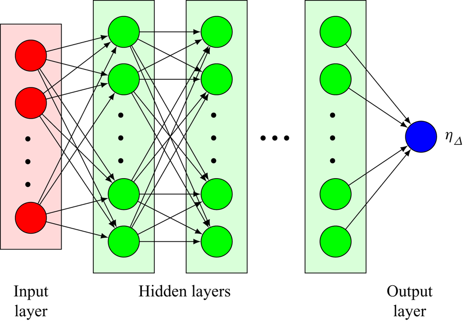
The schematic diagram of the ANN is shown in figure 1. The ANN is composed of multiple layers with many neurons. The neurons receive the input signals from the previous layer and send them to the next layer by the successive mathematical operation of the linear weighted sum and nonlinear activation. Each neuron in the  $l$th layer receives the inputs
 $X_j^{(l-1)}$ from the
 $(l-1)$th layer and then transmits them to the outputs
 $X_i^{(l)}$ activated by the nonlinear function. The transfer function from the
 $(l-1)$th layer to the
 $l$th layer is calculated as
 \begin{equation} X_i^{( l )} = \sigma \left[b_i^{( l )} + \sum_j {W_{ij}^{( l )}X_j^{( {l - 1} )}} \right], \end{equation}
where  $\sigma [ \cdot ]$ is the nonlinear activation function and
 ${W_{ij}^{( l )}}$ and
 $b_i^{( l )}$ are the weights and biases in the
 $l$th layer, respectively.
Schematic diagram of the ANN for predicting the KEF ratio  $\eta _{\varDelta }$.

The input features of the ANN are critical to the performance of predicting the KEF ratio  $\eta _\varDelta$. A set of input variables is listed in table 1 for different ANN models. The input variables for ANN models are dimensionless quantities, where several variables may be selected in compressible wall-bounded turbulence, such as
 ${\varDelta ^+ }, {y^+ }, {Re}_\varDelta$ and
 $\varDelta _\ell ^+$. In this paper,
 ${\varDelta ^+ } = {\bar \rho _w}{\tilde u_\tau }\varDelta /{\mu _w}$ is the normalized filter width,
 ${y^+ } = {{\bar \rho }_w}{\tilde u_\tau }y/{\mu _w}$ is the dimensionless normal distance,
 $Re_\varDelta = {{\bar \rho }_w}| {\tilde S} |{\varDelta ^2}/{\mu _w}$ is the mesh Reynolds number and
 $\varDelta _\ell ^+ = \varDelta /\ell$, with
 $\ell = {[ {\mu _w^3/( {\bar \rho _w^3\varepsilon } )} ]^{1/4}} = {[ {\mu _w^2/( {2\bar \rho _w^2\langle {{{\tilde S}_{ij}}{{\tilde S}_{ij}}} \rangle } )} ]^{1/4}}$. Here,
 ${\tilde u_\tau } = \sqrt {{\tau _w}/{{\tilde \rho }_w}}$ is the filtered wall friction velocity, where
 ${\tau _w} = {\mu _w}({{\partial \tilde u}}/{{\partial y}})$ is the wall shear stress, and
 $\langle \cdot \rangle$ denotes the spatial average along the homogeneous directions. In table 1, ANN1, ANN2 and ANN3 are the ANN models with input parameters normalized by the wall quantities (i.e.
 $\rho _w$ and
 $\mu _w$).
A set of inputs and outputs for different ANN models.

Apart from the dimensionless physical variables normalized by the wall quantities, we also select the dimensionless quantities using the semi-local normalization (Pecnik & Patel Reference Pecnik and Patel2017; Yang & Lv Reference Yang and Lv2018) as the input features of the ANN. The corresponding semi-local (SL) scaled variables include  $\varDelta _{SL}^+, y_{SL}^+, {Re}_{\varDelta, SL}$ and
 $\varDelta _{\ell, SL}^+$. Here, the semi-local scaled filter width is defined by
 $\varDelta _{SL}^+ = \bar \rho {\tilde u_\tau }\varDelta /\mu$,
 $y_{SL}^+ = \bar \rho {\tilde u_\tau }y/\mu$ is the semi-local scaled normal distance,
 ${Re}_{\varDelta,SL} = \bar \rho | {\tilde S} |{\varDelta ^2}/\mu$ is the local mesh Reynolds number and
 $\varDelta _{\ell,SL}^+ = \varDelta /{\ell _{SL}}$, where
 ${\ell _{SL}} = {[ {{\mu ^3}/( {{{\bar \rho }^3}\varepsilon } )} ]^{1/4}} = {[ {{\mu ^2}/( {2{{\bar \rho }^2}\langle {{{\tilde S}_{ij}}{{\tilde S}_{ij}}} \rangle } )} ]^{1/4}}$. Then, ANN1-SL, ANN2-SL and ANN3-SL represent the ANN models with input variables normalized by the semi-local physical quantities in table 1.
A total of four layers (an input layer, two hidden layers and an output layer) with neurons in the ratio  $M:100:100:1$ are chosen in this paper, where
 $M$ is the number of input variables listed in table 1. The activation functions of the hidden layers and output layer are the hyperbolic tangent function (tanh) and linear function, respectively, which are defined by
 \begin{equation} {\sigma _h}( x ) = \frac{\mathrm{e}^x - \mathrm{e}^{{-}x}} {\mathrm{e}^x + \mathrm{e}^{{-}x}}, \quad {\sigma _o}( x ) = x. \end{equation}
The mean-squared error (MSE) function is selected as the loss function of the ANN, which is defined as  $L = \langle ( {\eta _\varDelta ^{true} - \eta _\varDelta ^{pred}} )^2 \rangle$, where
 $\eta _\varDelta ^{true}$ and
 $\eta _\varDelta ^{pred}$ denote the true and predicted values of the ANN, respectively. A total of
 $2 \times {10^4}$ samples are selected from 20 snapshots of the filtered DNS data with a ratio of the filter width
 $\varDelta /{\varDelta _{DNS}}$ ranging from 2 to 20 (i.e.
 $\varDelta /{\varDelta _{DNS}} \in \{ {2,4,\ldots,20} \}$). We use the cross-validation strategy and divide the dataset into a training set and a testing set to suppress parameter overfitting of the ANN; 70 % of the samples are randomly extracted from the total dataset and are used as the training set, while the others are used for testing. The weights of the ANN are initialized by the Glorot-uniform algorithm and optimized by the Adam algorithm (Kingerma & Ba Reference Kingerma and Ba2019) for
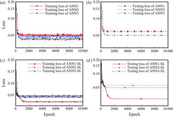
 $1 \times {10^4}$ iterations, with a batch size and learning rate of 1000 and 0.01, respectively. The grid search method is chosen as the hyperparameter pruning method of the ANN to determine the optimal hyperparameters, such as the numbers of layers and neurons and the types of activation functions. The learning curves of the ANN models for different input variables using different normalization methods are shown in figure 2. After a long training with
 $1 \times 10^4$ epochs, the MSE losses in both the training sets and testing sets converge quickly and gradually reach stationarity. The training loss and testing loss for both wall quantity normalization and semi-local scaling methods are very close, which means that the selected hyperparameters are reasonable and all the ANN models are well trained.
Learning curves of the proposed ANN models for predicting the KEF ratio  $\eta _\varDelta$: (
 $a$) training loss for ANN models, (
 $b$) testing loss for ANN models, (
 $c$) training loss for ANN-SL models and (
 $d$) testing loss for ANN-SL models.

We evaluate the performance of different ANN models by calculating three metrics to measure the difference between the true value ( $\eta _\varDelta ^{real}$) obtained from the filtered DNS data and the predicted value (
 $\eta _\varDelta ^{model}$) calculated by the ANN models. They are the correlation coefficient
 $C(\eta _\varDelta )$, the relative error
 $E_r(\eta _\varDelta )$ and the ratio of the root-mean-square value
 $R(\eta _\varDelta )$, which are expressed, respectively, as
 $$\begin{gather} C({\eta _\varDelta }) = \frac{{\langle {( {\eta _\varDelta^{{{real}}} - \langle {\eta _\varDelta^{{{real}}}} \rangle } )( {\eta _\varDelta^{{{model}}} - \langle {\eta _\varDelta^{{{model}}}} \rangle } )} \rangle }}{{{{\langle {{{( {\eta _\varDelta^{{{real}}} - \langle {\eta _\varDelta^{{{real}}}} \rangle } )}^2}} \rangle }^{1/2}}{{\langle {{{( {\eta _\varDelta^{{{model}}} - \langle {\eta _\varDelta^{{{model}}}} \rangle } )}^2}} \rangle }^{1/2}}}}, \end{gather}$$
 $$\begin{gather}{E_r}( {{\eta _\varDelta }} ) = \frac{{{{\langle {{{( {\eta _\varDelta^{{{real}}} - \eta _\varDelta^{{{model}}}} )}^2}} \rangle }^{1/2}}}}{{{{\langle {{{( {\eta _\varDelta^{{{real}}}} )}^2}} \rangle }^{1/2}}}}, \end{gather}$$
 $$\begin{gather}R( {{\eta _\varDelta }} ) = \frac{{{{\langle {{{( {\eta _\varDelta^{{{model}}} - \langle {\eta _\varDelta^{{{model}}}} \rangle } )}^2}} \rangle }^{1/2}}}}{{{{\langle {{{( {\eta _\varDelta^{{{real}}} - \langle {\eta _\varDelta^{{{real}}}} \rangle } )}^2}} \rangle}^{1/2}}}}. \end{gather}$$
The results with high correlation coefficients, low relative errors and high ratios of root-mean-square values indicate successful modelling.
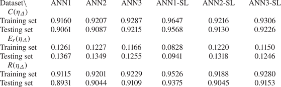
Table 2 shows comparisons of the correlation coefficients, relative errors and ratios of root-mean-square values for the KEF ratio  $\eta _\varDelta$ in both training and testing sets after the 10 000-iteration training process. The results of the training and testing sets show slight differences, which indicates that none of the trained ANN models with different inputs are overfitted. Furthermore, the metrics predicted by the semi-local normalization obviously outperform those normalized by the wall quantities, especially for the case of ANN1-SL. The ANN1-SL model performs better than the other five ANN models. The correlation coefficient and relative error of the ANN1-SL model in the testing dataset are 96 % and 9.4 %, respectively. The ratio of the root-mean-square value of the ANN1-SL model is equal to 0.94 and very close to 1, which indicates that the ANN1-SL model can accurately reconstruct the KEF ratio. In contrast to other ANN models, we take the local mesh Reynolds number instead of the normalized filter width in the input of the ANN1-SL model. The prediction performance improves to some degree. More importantly, ANN1-SL can be more easily generalized to other types of compressible wall-bounded turbulence.
Correlation coefficient ( $C$), relative error (
 $E_r$) and ratio of root-mean-square value (
 $R$) of the KEF ratio
 $\eta _\varDelta$ in different datasets for different ANN models.

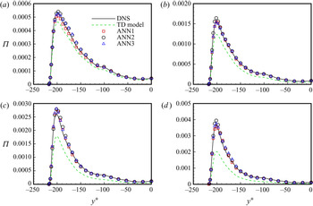
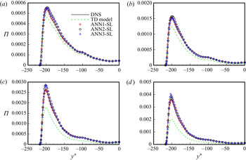
Comparisons of the KEF reconstructed by different ANN models and that from the TD model along the normal direction with different filter widths ( $\varDelta /\varDelta _{DNS}=4$, 8, 12, 16) are shown in figures 3 and 4. The magnitudes of the KEF obtained from the TD model with these filter widths are obviously different from the real value, even though their shapes are very similar due to the high correlation coefficients. The KEF modelled by the ANN models is very close to the DNS data, and the six ANN models show similar results. Since the ANN1-SL model demonstrates the better a priori accuracy among these ANN models, we can also use the ANN1-SL model to reconstruct the KEF ratio
 $\eta _\varDelta$ in the KCM as the representation of these ANN models. The newly constructed KEF model here is a semi-explicit model.
Comparisons of the KEF reconstructed by different ANN models using wall-quantity normalization along the normal direction with different filter widths: ( $a$)
 $\varDelta /\varDelta _{DNS}=4$; (
 $b$)
 $\varDelta /\varDelta _{DNS}=8$; (
 $c$)
 $\varDelta /\varDelta _{DNS}=12$; and (
 $d$)
 $\varDelta /\varDelta _{DNS}=16$.

Comparisons of the KEF reconstructed by different ANN models using semi-local normalization with different filter widths: ( $a$)
 $\varDelta /\varDelta _{DNS}=4$; (
 $b$)
 $\varDelta /\varDelta _{DNS}=8$; (
 $c$)
 $\varDelta /\varDelta _{DNS}=12$; and (
 $d$)
 $\varDelta /\varDelta _{DNS}=16$.

5. Results of applications
5.1. Application in compressible turbulent channel flows
In this section, the KCM will be verified in compressible turbulent channel flows, and the case setting of the LES is the same as that of the DNS in § 4. The filtered Navier–Stokes equations (2.1)–(2.3) are solved using a high-precision non-dimensional finite-difference solver in Cartesian coordinates: the equations are temporally integrated using the third-order Runge–Kutta scheme, and a sixth-order central-difference scheme is used for the discretization of both the convective and viscous terms.
In this study, we will select three commonly used SGS models for comparison, namely the Vreman model, WALE model and DSM. In the DSM,  $C_{sm}, C_I$ and
 $Pr_T$ are solved dynamically based on the Germano identity. Following the form of the Vreman model in compressible turbulence (Sayadi & Moin Reference Sayadi and Moin2012; Zhang, Wan & Sun Reference Zhang, Wan and Sun2019), the model coefficient
 $C_v=2.5C_{sm}^2$, where
 $C_{sm}=0.1$. The WALE model here is taken in the same form as in Garnier, Adams & Sagaut (Reference Garnier, Adams and Sagaut2000). The model coefficient of WALE is
 $C_w=10.6C_{sm}^2$, and
 $C_{sm}$ is also taken as 0.1. In Garnier et al. (Reference Garnier, Adams and Sagaut2000), Sayadi & Moin (Reference Sayadi and Moin2012) and Zhang et al. (Reference Zhang, Wan and Sun2019), the isotropic parts of the Vreman and WALE models are ignored, and we also adopt
 $C_I=0$ for the Vreman and WALE models here. The SGS Prandtl number
 $Pr_T$ of the Vreman model, WALE model and KCM can be evaluated as 0.9 empirically (Georgiadis, Alexander & Reshotko Reference Georgiadis, Alexander and Reshotko2001; Sayadi & Moin Reference Sayadi and Moin2012; Zhang et al. Reference Zhang, Wan and Sun2019). The filtering procedure is also performed using a top-hat filter. The grid filter width is
 $\varDelta =(\varDelta _x\varDelta _y\varDelta _z)^{1/3}$, with
 $\varDelta _x, \varDelta _y$ and
 $\varDelta _z$ representing the local grid width along the three axes, and the test-filter width is set as
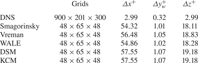
 $2\varDelta$. But the Vreman model is implemented using the filter width in each direction according to its model form. The details of the grid settings are listed in table 3.
Parameters of the simulations in compressible channel flow ( $Ma=1.5, Re=3000, Re_{\tau }=220$).

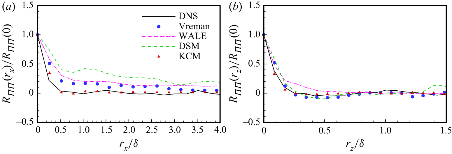
Spatial correlation coefficients of KEF can reveal the prediction ability of SGS models on the spatial structures of KEF. Figure 5( $a{,}b$) shows the streamwise and spanwise two-point correlation coefficients of KEF at various locations of
 $y^+=50$, respectively. The two-point correlation coefficient of KEF can be defined as
 \begin{equation} R_{\varPi\varPi}(\boldsymbol r)=\frac{\varPi (\boldsymbol x)\varPi (\boldsymbol x+\boldsymbol r)}{\varPi (\boldsymbol x)\varPi (\boldsymbol x)}. \end{equation}
Two-point correlation coefficients of KEF at various locations of  $y^+=50$: (
 $a$) streamwise correlation; and (
 $b$) spanwise correlation. DNS (black solid line), Vreman (blue circles), WALE (pink dash-double dotted line), DSM (green dashed line) and KCM (red triangles).

From figure 5, we can see that both the streamwise and spanwise two-point correlation coefficients of KEF from KCM are much closer to the real values than other models, indicating that KCM gives a good modelling of the main spatial distribution characteristics of KEF.
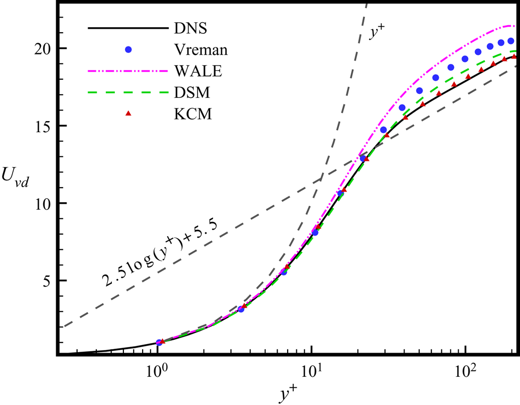
The distribution of the van Driest transformed mean streamwise velocity ( $U_{vd}=\int _{0}^{U}\!\sqrt {\langle \rho \rangle /\rho _w}\, \textrm {d} \langle U\rangle$) as a function of
 $y^+$ is displayed in figure 6, and the results obtained from DNS, KCM and some representative eddy-viscosity models, including DSM, Vreman and WALE (Germano et al. Reference Germano, Piomelli, Moin and Cabot1991; Nicoud & Ducros Reference Nicoud and Ducros1999; Vreman Reference Vreman2004) are compared together. As expected for
 $y^+<5$, the mean streamwise velocity generally increases linearly with
 $y^+$. Additionally, almost all the results from the SGS models collapse to the DNS result in the viscous sublayer and up to part of the buffer region (
 $y^+<20$). In the log-law region, the KCM still provides a perfect estimation of
 $U_{vd}$, but the results of other SGS models show an obvious deviation from the DNS result. Furthermore, from figure 6, we know that the KCM provides proper SGS dissipation, but the other typical eddy-viscosity SGS models exhibit excessive SGS dissipation.
Van Driest transformed mean velocity files from different SGS and result from DNS for comparison.

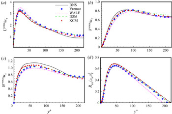
Figure 7(a)–(c) shows the profiles of the normalized resolved turbulence intensities  $\tilde {u}_i^{rms}/{u_{\tau }}=\langle (\tilde {u}_i-\langle \tilde {u}_i\rangle )^2 \rangle ^{1/2}/{u_{\tau }}$ calculated from the LES data of several SGS models, including Vreman, WALE, DSM and KCM, and the result from DNS is also provided for comparison. Figure 7(
 $a$) shows the streamwise turbulence intensity
 $U^{rms}$, and we can see that the result of the KCM is obviously in better agreement with the DNS result than the results of the other models, especially in the buffer region. Additionally, the wall-normal turbulence intensity
 $V^{rms}$ and spanwise turbulence intensity
 $W^{rms}$ are shown in figure 7(b,c), respectively. As seen from the two panels, all the SGS models have low performance, but the results of KCM have a slight advantage over those of the other SGS models. Figure 7(
 $d$) shows the distribution of the normalized Reynolds stress
 $R_{uv}$ along the normal height
 $y^+$, and the results of DNS, Vreman, WALE, DSM and KCM are compared together. The Reynolds stress can be expressed as
 \begin{equation} R_{ij} =\langle \rho \rangle(\{ u_i u_j \}-\{ u_i \}\{ u_j \} ), \end{equation}
where  $\{\cdot \}$ denotes the Favre averaging and
 $\{\phi \}={\langle \rho \phi \rangle }/{\langle \rho \rangle }$.
Turbulence intensities and the Reynolds stress normalized by the friction velocity  $u_{\tau }$ from DNS and different models: (
 $a$) streamwise turbulence intensity; (
 $b$) wall-normal turbulence intensity; (
 $c$) spanwise turbulence intensity; and (
 $d$) Reynolds stress.

For turbulent flows, the property of ergodicity is assumed, and thus  $\langle \phi \rangle = \langle \bar \phi \rangle$. Then, the Reynolds stress can also be expressed as
 \begin{equation} R_{ij}=\langle \bar{\rho} \rangle(\{ \widetilde{u_i u_j}\}- \{ \tilde{u}_i \}\{ \tilde{u}_j \} )=R_{ij}^{LES}+\langle \tau_{ij} \rangle, \end{equation}
where
 \begin{equation} R_{ij}^{LES}=\langle \bar{\rho} \rangle(\{\tilde{u}_i\tilde {u}_j\}-\{\tilde{u}_i\}\{\tilde {u}_j\}) \end{equation}
is the resolved Reynolds stress and  $\tau _{ij}$ is the SGS stress.
In contrast to the results of other SGS models, the KCM gives a perfect total Reynolds stress  $R_{uv}$ in almost all of the regions. The results in figure 7 demonstrate that the KCM can also better predict the high-order statistics of turbulence.
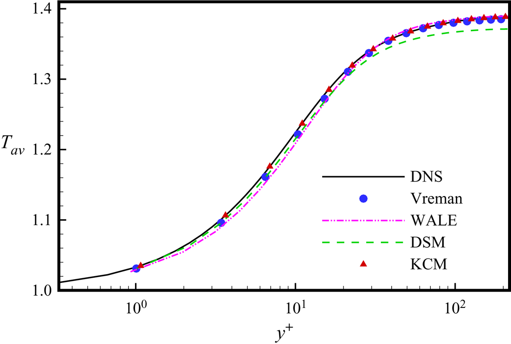
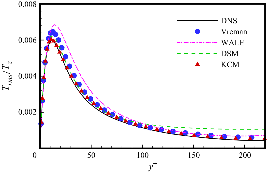
The mean temperature obtained from DNS and the four SGS models are also compared together in figure 8. KCM shows the best behaviour, and the result from Vreman is better than those of the other two models. Figure 9 displays the profiles of the normalized resolved temperature fluctuation  $\tilde {T}^{rms}/{T_{\tau }}=\langle (\tilde {T}-\langle \tilde {T_i}\rangle )^2 \rangle ^{1/2}/{T_{\tau }}$ along the wall-normal direction from DNS and these SGS models, where
 $T_{\tau }=q_w/\rho _wc_pu_{\tau }$, with
 $q_w=-k({{\partial \tilde T}}/{{\partial y}})$ the friction temperature. The result of KCM is very close to the real value, and is better than those of other models. The temperature–velocity correlation can be written as
 \begin{equation} R_{u_iT}=\langle \bar{\rho} \rangle(\{ \widetilde{u_i T}\}-\{ \tilde{u}_i \}\{ \tilde{T} \} )=R_{u_iT}^{LES}+\langle Q_i \rangle, \end{equation}
where
 \begin{equation} R_{u_iT}^{LES}=\langle \bar{\rho} \rangle(\{\tilde{u}_i\tilde T\}-\{\tilde{u}_i\}\{\tilde T\}) \end{equation}
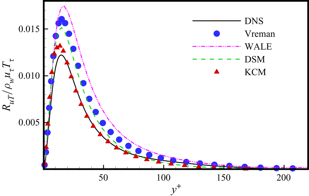
is the resolved temperature–velocity correlation and  $Q_i$ is the SGS heat flux. We show the normalized temperature–velocity correlation in figure 10, and we find that the result from KCM is much closer to the real value compared with other traditional eddy-viscosity SGS models. Thus, the reasonable eddy viscosity of KCM will improve the prediction of the SGS heat-flux model.
Mean temperature profiles obtained from DNS and different SGS models.

Temperature fluctuation normalized by friction temperature  $T_{\tau }$ from DNS and different SGS models.

Normalized temperature velocity correlation from DNS and different SGS models.

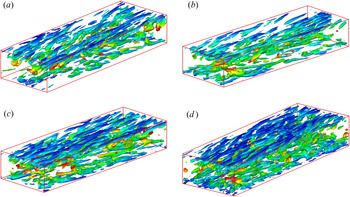
Accurate prediction of turbulent structure is also an important ability for the new SGS model. We show in figure 11(a–d) the instantaneous isosurface of  $Q$ (second invariant of the strain-rate tensor,
 $Q=0.2$) obtained from Vreman, WALE, DSM and KCM, respectively. Comparing the four pictures, we find that the result of the KCM shows more small-scale and abundant structures, especially in the near-wall region. Nevertheless, the results of the other models show larger tube-like structures and lack small-scale structures. These observations also indicate that the KCM has the advantage of accurately predicting the turbulent structure.
Instantaneous isosurface of  $Q$ (second invariant of the strain-rate tensor,
 $Q=0.2$) obtained from (
 $a$) Vreman, (
 $b$) WALE, (
 $c$) DSM and (
 $d$) KCM in compressible turbulent channel flow.

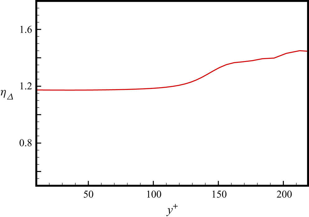
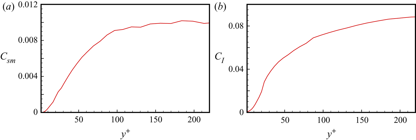
Then, we need to check the performance of the KEF ratio and the model coefficients in an a posteriori test of compressible turbulent channel flow. Figure 12 shows the KEF ratio  $\eta _{\varDelta }$ of KCM in the compressible turbulent channel flow;
 $\eta _{\varDelta }$ is almost constant for
 $y^+<120$, and the value is approximately 1.16. For
 $y^+>120$, it will grow slowly. Figure 13(a,b) displays the model coefficients
 $C_{sm}$ and
 $C_I$, respectively. It is shown that the curves of
 $C_{sm}$ and
 $C_I$ are similar to each other. They grow rapidly from zero near the wall, and remain nearly constant in the centre region of the channel.
An a posteriori test of KEF ratio  $\eta _{\varDelta }$ of KCM in compressible channel flow.

An a posteriori test of the model coefficients of KCM in compressible turbulent channel flow: ( $a$)
 $C_{sm}$ and (
 $b$)
 $C_I$.

5.2. Application in compressible flat-plate boundary layer
To verify the KCM in simulating more complex compressible wall flow, we select the compressible flat-plate boundary layer as a typical example. Compared with the channel flow, the flat-plate boundary layer is a more complicated type of wall-bounded flow. Flat-plate boundary layer flow is a typical flow consisting of laminar, transitional and fully turbulent regions, which is a common phenomenon in wall flow. Thus, it can be regarded as a classical case for evaluating the performance of the new SGS model in transitional and turbulent flows. The LES of the transition to turbulence of the flat-plate boundary layer has been frequently investigated over an extended period (Ducros, Comte & Lesieur Reference Ducros, Comte and Lesieur1996; Huai et al. Reference Huai, Joslin and Piomelli1997; Sayadi & Moin Reference Sayadi and Moin2012).
In this paper, we choose a spatially developing supersonic adiabatic flat-plate boundary layer flow (Pirozzoli, Grasso & Gatski Reference Pirozzoli, Grasso and Gatski2004) (at  $Ma=2.25$ and
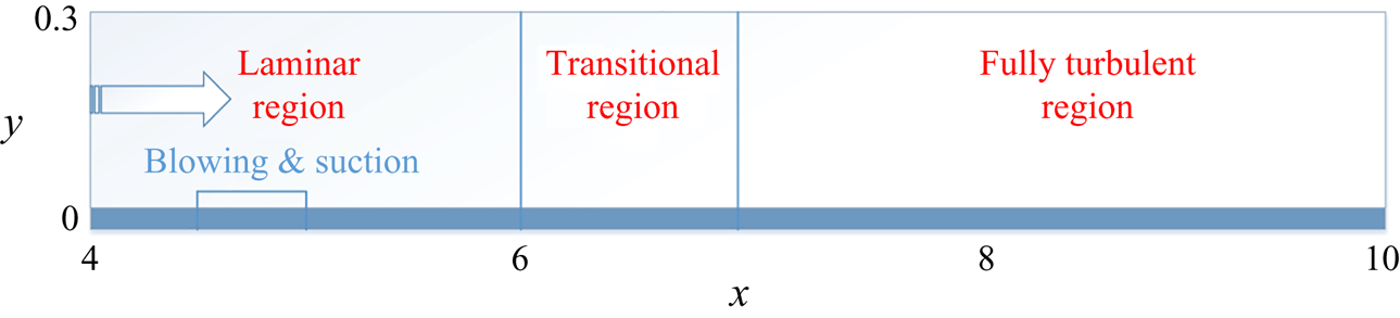
 $Re_{\theta }\approx 4000$) to test the new model; a sketch of the computational domain for the numerical simulation is shown in figure 14. The computational domain (see figure 14) is bounded by in-flow and out-flow boundaries, a wall boundary, a far-field boundary and the two boundaries (periodic) in the spanwise direction; the computational domain has a size of
 $L_x\times L_y\times L_z=6\times 0.3\times 0.175$. Blowing and suction disturbances are imposed at the wall with an interval of x (
 $4.5\leq x\leq 5.0$). The form of blowing and suction is the same as that in (Pirozzoli et al. Reference Pirozzoli, Grasso and Gatski2004) except for the magnitude of the amplitude. To simulate a natural transition, an amplitude of 0.02 is selected in this case. The grid resolution for the DNS of this example case is
 $10\,090 \times 90 \times 320$, and
 ${\rm \Delta} x^+\times {\rm \Delta} y^+\times {\rm \Delta} z^+=6.02 \times 0.58 \times 5.47$ in the streamwise, wall-normal and spanwise directions.
Sketch of the computational domain of the flat-plate boundary layer for the numerical simulation.

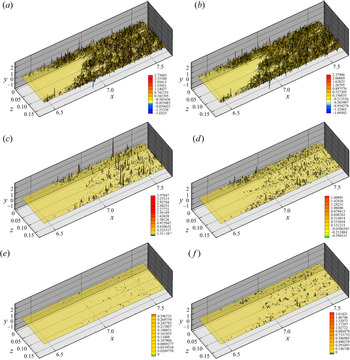
The newly proposed LES model KCM is tested a priori using the DNS data of the compressible flat-plate flow first. To directly explain the difference between the KEF constrained eddy-viscosity model KCM and the traditional eddy-viscosity models (i.e. the SM, WALE model, etc.) on the prediction of the spatial distribution of KEF, a priori tests of the energy fluxes obtained from KCM, SM, DSM, Vreman and WALE and the real value are compared in figure 15. In the a priori tests, the DNS data of the transition to the turbulence region at  $y^+=15$, which is in the buffer region, are filtered in the spanwise direction with a top-hat filter, and the filter width is
 $\bar {\varDelta }=8\varDelta _z$. From figure 15, we find that the spatial distribution of KEF obtained from the KCM is very similar to that of the real value in terms of both phase and amplitude. In contrast, the KEF distributions obtained from the other three traditional eddy-viscosity models and DSM have a significant difference from the real KEF distribution. Except for the weak negative KEF in the result from DSM, there are not any backscatters in the results from other traditional eddy-viscosity models. This result indicates that the strong ability of the KCM on the accurate prediction of KEF is valid for the transition and turbulence of the flat-plate boundary layer.
An a priori test of the local KEF of the compressible flat-plate boundary layer at  $y^+=15$ from different SGS models, and the real value for comparison:
 $(a)$ the real value;
 $(b)$ KCM;
 $(c)$ SM;
 $(d)$ DSM;
 $(e)$ Vreman; and
 $(\,f)$ WALE.

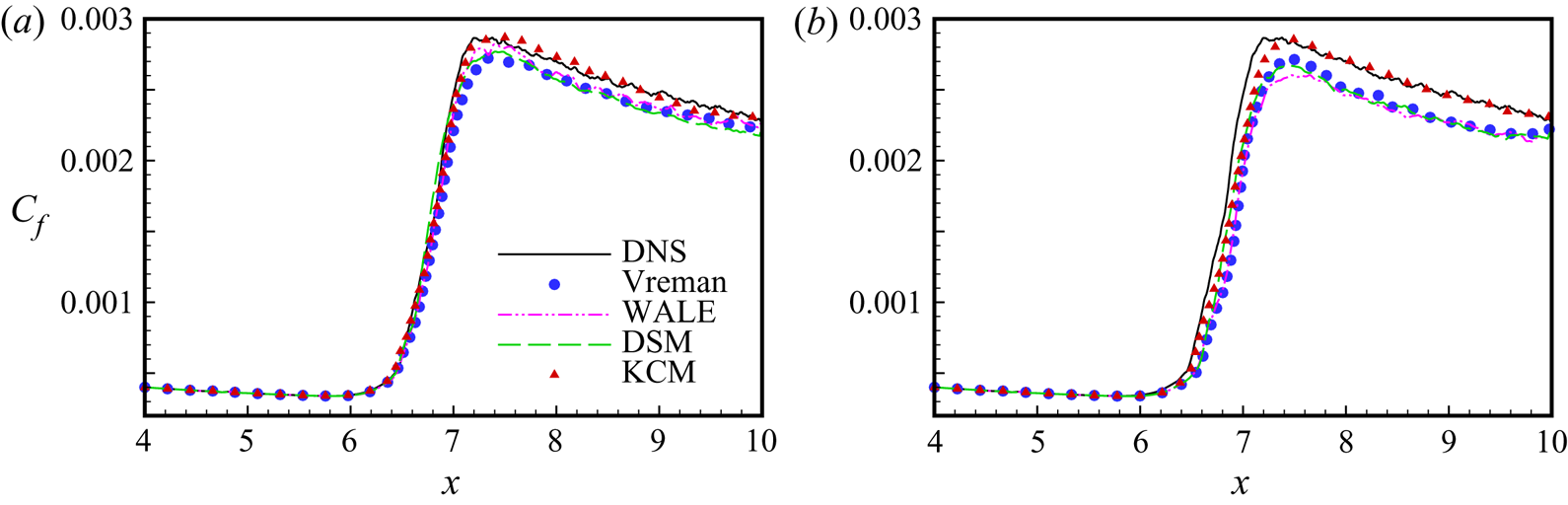
Then, for the a posteriori test, the numerical scheme is the same as that for the LES of the turbulent channel flow in § 5.1. In this case, we choose two sets of grids for the LES of the compressible flat-plate boundary layer; the parameter settings are shown in table 4. In figure 16, we show the distributions of the skin-friction coefficients obtained from Vreman, WALE, DSM and KCM compared with the results obtained from DNS on the two sets of grids. In figure 16, from the curve of the real skin-friction coefficient, we can see that the occurrence of the transition is at  $x\approx 6.3$, the transition peak is reached at
 $x\approx 7.2$, and then the steady turbulence region is gradually approached as the boundary layer flow develops into fully developed turbulence. It is easy to see that all the models can predict the point of transition properly in figure 16(
 $a$); however, the result of the KCM still has a small advantage compared with the other results. Under the coarser grid, we find that the KCM still predicts the transition point and transition peak well, as shown in figure 16(
 $b$), and it has an obvious advantage compared with the other models. The traditional wall-bounded turbulence model cannot predict the transition (Sayadi & Moin Reference Sayadi and Moin2012; Zhou et al. Reference Zhou, Li, Qi and Yu2019a), but the SM constrained by KEF (KCM) can predict laminar, transitional and turbulent flow regions accurately and can provide appropriate SGS dissipation in different flow regions. The primary reason for this observation is that the KCM can supply the proper KEF in different regions.
Skin-friction coefficient distribution along the flat plate: ( $a$) grid-1 and (
 $b$) grid-2.

Parameters of the simulations in the supersonic transition and turbulent flat-plate boundary layer ( $Ma=2.25, Re=635\,000$).

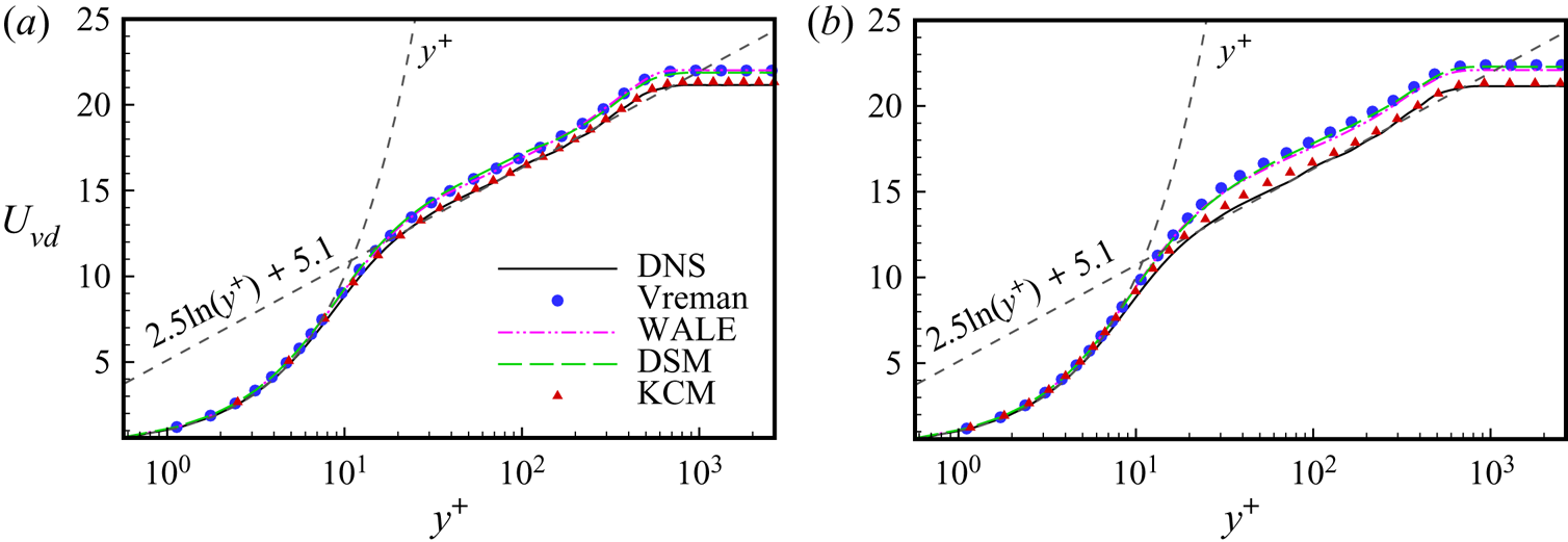
Moreover, the distribution of the van Driest transformed mean streamwise velocity at  $x=8.8$ under the different scales of the grids are shown in
figure 17( $a$,
 $b$), where the flow can be regarded as steady turbulence. As seen from the two panels, both of the profiles predicted by KCM are always very close to the real values in all the regions. Conversely, the other models clearly overestimate the velocity in the buffer region, log-law region and defect-law region.
Van Driest transformed mean streamwise velocity at  $x=8.8$: (
 $a$) grid-1 and (
 $b$) grid-2.

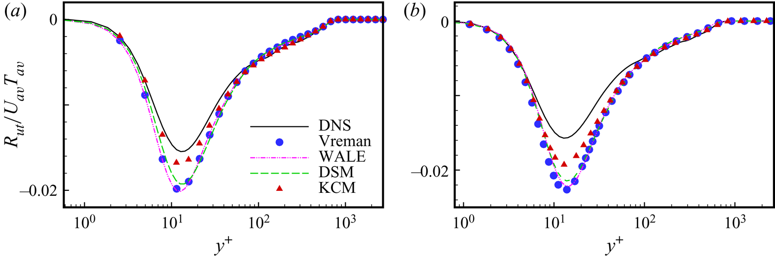
In figure 18(a,b), we display the normalized temperature–velocity correlation along the wall-normal direction at  $x=8.8$ for the two grid resolutions. In contrast to other models, the result from KCM in the case of the fine grid has the obvious advantage, but this is not so distinct in the coarse-grid case.
Temperature–velocity correlation normalized by the product of averaged temperature and velocity ( $u_{av}T_{av}$) along the wall-normal direction at
 $x=8.8$ of the compressible flat-plate boundary layer: (
 $a$) grid-1 and (
 $b$) grid-2.

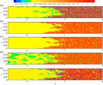
Figure 19 shows the a posteriori test of the local KEF obtained from the LES data of Vreman, WALE, DSM and KCM in the case of grid-1; the real KEF is also displayed here for comparison. From the figure, we find that the results are similar to those in the a priori test. The KEF from KCM and the real KEF have similar spatial distributions, and the backscatters are full of their flow fields. Even if the KEF obtained from DSM exist some weak local energy backscatters, the distribution of the local KEF is still greatly different from the real value. On the other hand, the KEF obtained from the traditional eddy-viscosity models still has no backscatter in the whole field, and the amplitudes of the forward cascades are higher than the real value, which indicates that the SGS models are more dissipative. Additionally, we can infer that KCM can predict KEF, energy backscatters and flow structures more accurately in this case.
An a posteriori test of the local KEF of the compressible flat-plate boundary layer at  $y^+=15$ from the LES models in the case of grid-1, and the real value for comparison:
 $(a)$ the real value;
 $(b)$ Vreman;
 $(c)$ WALE;
 $(d)$ DSM; and
 $(e)$ KCM.

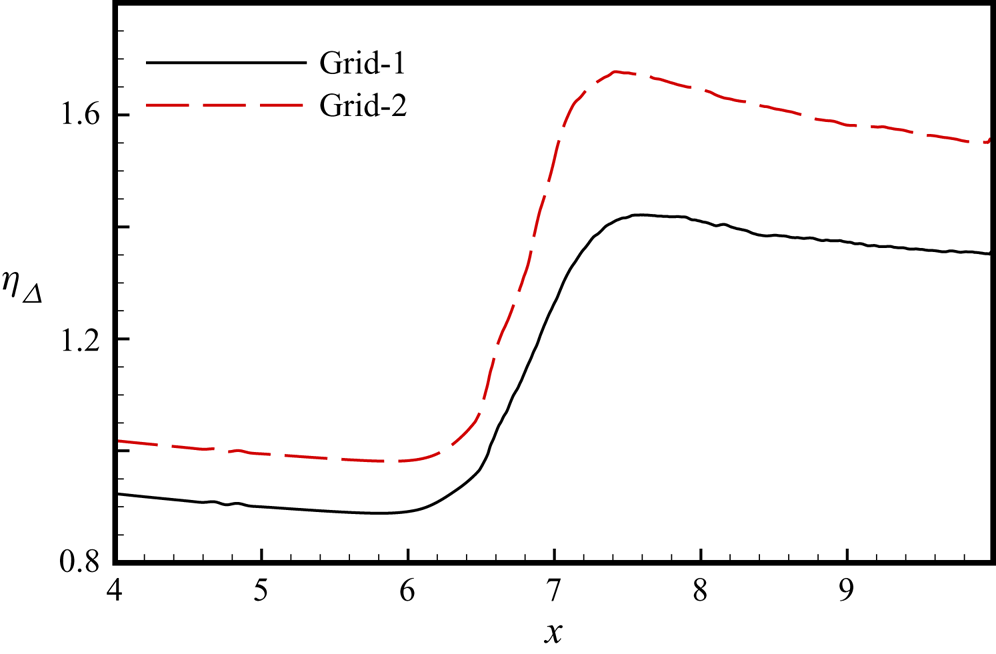
Figure 20(a,b) shows the KEF ratio  $\eta _{\varDelta }$ of KCM along the streamwise direction at
 $y^+=15$ of the compressible flat-plate boundary layer in the two cases of different grid resolutions. The distribution trend of the KEF ratio is similar to that of the skin-friction coefficient in figure 16. Moreover, the value of
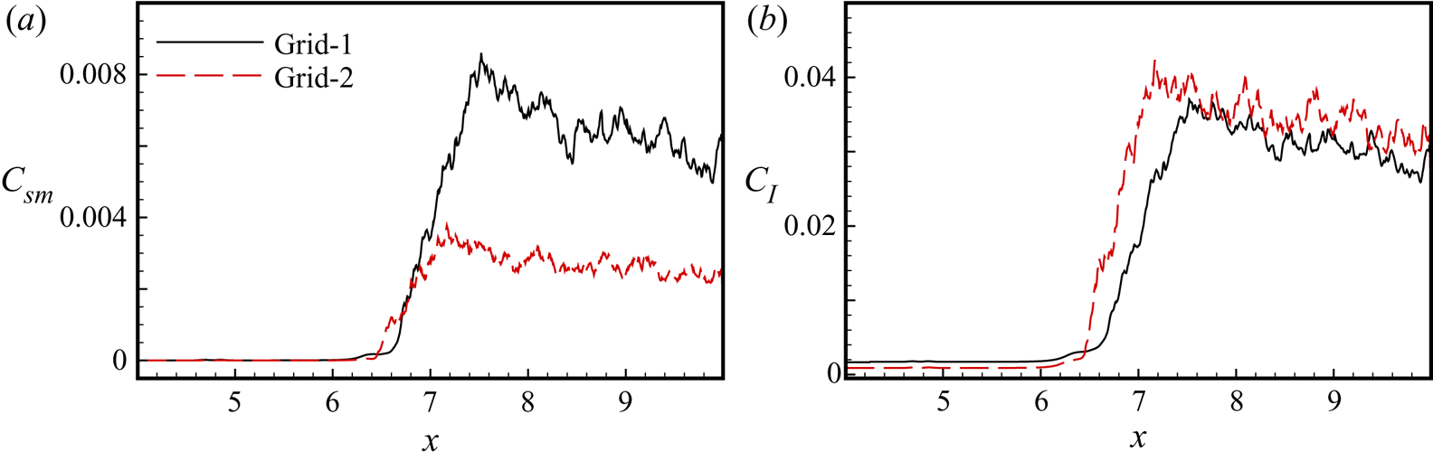
 $\eta _{\varDelta }$ in the coarse-grid case is higher that in the fine-grid case, which also indicates that the proposed model will be much better than the model with the constraint from the original TD model on the coarse mesh. Figure 21 shows the model coefficients of the two cases with different grid resolutions. In the region
 $4\lt x\lt 6.5$, all the model coefficients of the two cases are zero. It could also indicate that KCM is off in the laminar flow, and starts to work at the transition point. Also, the distributions of these model coefficients are similar to the distributions of the skin-friction coefficient.
An a posteriori test of KEF ratio  $\eta _{\varDelta }$ of KCM along the streamwise direction at
 $y^+=15$ of the compressible flat-plate boundary layer at different grid resolutions: (
 $a$) grid-1 and (
 $b$) grid-2.

An a posteriori test of the model coefficients of KCM along the streamwise direction at  $y^+=15$ of the compressible flat-plate boundary layer at different grid resolutions: (a)
 $C_{sm}$ and (b)
 $C_I$.

6. Conclusions
In this paper, we propose a kinetic-energy-flux-constrained model (KCM) for the large-eddy simulation (LES) of compressible wall turbulent flows. The new proposed subgrid-scale (SGS) stress model aims to guarantee the proper prediction of the kinetic energy flux (KEF) and the robustness of the computation in LES of compressible wall-bounded turbulence. The KEF obtained from the tensor-diffusivity (TD) model has a high correlation with the real value, but the TD model has low numerical stability. In contrast, the KEF from the Smagorinsky model (SM) has a low correlation with the real value but has a high robustness in computation. At the same time, from theoretical analyses, we can confirm that the SM still has higher numerical stability than the TD model, even in the condition with the same SGS dissipation. Using the DNS data of compressible channel flow, through an artificial neural network (ANN), we obtain the KEF ratio between the KEF from the TD model and the real value. Thus, the modelled KEF is obtained and then applied to constrain the SM. In addition, the ANN method is only applied to predict a dimensionless coefficient, which might be easy to generalize to the simulation of other turbulent flows.
The KCM is first applied to the simulation of compressible turbulent channel flow. Compared with other traditional eddy-viscosity SGS models, the KCM could more accurately predict typical statistical quantities, including the mean streamwise velocity, Reynolds stress, temperature–velocity correlation, etc. Furthermore, the new model can predict more abundant coherent turbulent structures in the channel flow. Then, the KCM is also tested in a supersonic spatially developing flat-plate flow. Through an a priori test, the feasibility of the KCM for LES of more complex wall-bounded turbulence is displayed. In an a posteriori test, the KCM could precisely predict the natural transition process, including the onset of transition and the transition peak. Moreover, the KCM could provide more accurate profiles of skin friction, the mean velocity profiles and temperature–velocity correlation in cases with two different grid resolutions. The new model could also predict the energy backscatters in transition and turbulent flows properly.
In summary, the new LES methodology suggested in this paper has been verified to be an effective method in LES. It can help to improve the prediction of both kinetic energy flux and SGS heat flux. Nevertheless, it should be mentioned that the new methodology still needs to be tested and modified in the wall-bounded turbulence with other types of complex-geometry boundaries.
Acknowledgements
The authors thank the National Supercomputer Center in Tianjin (NSCC-TJ) and the National Supercomputer Center in GuangZhou (NSCC-GZ) for providing computer time.
Funding
This work was supported by the National Key Research and Development Program of China (2020YFA0711800 and 2019YFA0405302) and NSFC Projects (Nos. 12072349, 91852203 and 91952104).
Declaration of interests
The authors report no conflict of interest.