1. Introduction
The Reynolds-averaged Navier–Stokes (RANS) method, coupled with turbulence models, remains the workhorse tool in industrial applications owing to its computational efficiency and tractability (Witherden & Jameson Reference Witherden and Jameson2017). However, the predictive accuracy of the RANS method depends critically on the turbulence model for the Reynolds stress (Xiao & Cinnella Reference Xiao and Cinnella2019), which accounts for the influences of velocity fluctuations on mean flows. Conventional turbulence models often fail to generalise across different flow regimes, e.g. separated flows, and typically require manual calibration of empirical model coefficients. Therefore, it is necessary to develop more generalisable turbulence models that remain reliable across a wide range of flow scenarios.
Turbulence models have been developed over the past century with the ultimate goal of establishing a unified model applicable to a broad range of flows (Prandtl Reference Prandtl1925; Lumley Reference Lumley1970; Liu et al. Reference Liu, Wang, Zhao and Xiao2026b ). The most widely used turbulence models are based on the Boussinesq assumption, which assumes that the Reynolds stress anisotropy is aligned with the mean strain rate and scaled by an eddy viscosity coefficient. Various eddy viscosity models have been proposed, from the algebraic mixing length model (Prandtl Reference Prandtl1925) to the transport-equation-based models (Wilcox Reference Wilcox2008), which are formulated primarily based on the equilibrium behaviour of canonical turbulent flows (Pope Reference Pope2000), e.g. the logarithmic law of the wall. These models can perform well in canonical flows and have been used in many engineering applications (Menter Reference Menter1994). An alternative modelling approach is based on the Reynolds stress transport equation (Chou Reference Chou1945; Launder et al. Reference Launder, Reece and Rodi1975), which describes the physical evolution of the Reynolds stress tensor. This approach relaxes the Boussinesq assumption but faces difficulties in the numerical stiffness and the modelling of higher-order terms, particularly the slow and rapid pressure-strain correlations (Rotta Reference Rotta1951; Launder et al. Reference Launder, Reece and Rodi1975). For improved numerical robustness, the explicit algebraic Reynolds stress model (EARSM) (Wallin & Johansson Reference Wallin and Johansson2000) is derived from the Reynolds stress transport equation under the weak-equilibrium assumption that neglects the temporal variation of the Reynolds stress anisotropy. Compared with the linear eddy viscosity model, such algebraic Reynolds stress models can provide more accurate predictions at a similar computational cost for flows with strong Reynolds stress anisotropy, e.g. secondary flows. However, they still have difficulties in generalising across diverse flow regimes, particularly with boundary layer separation where the underlying equilibrium assumptions break down. Hence, a broadly generalisable turbulence model remains elusive and requires further development.
Machine learning methods (Duraisamy et al. Reference Duraisamy, Iaccarino and Xiao2019) have emerged as a promising tool for constructing generalisable Reynolds stress closures based on high-fidelity data. These approaches typically seek an optimal functional mapping for the Reynolds stress by minimising discrepancies between model predictions and available flow data. The Reynolds stress closure can be represented with neural networks, given their great approximation capability and training efficiency. Machine learning-augmented turbulence closures have been shown to improve RANS predictions in one class of flows similar to the training case (Ling et al. Reference Ling, Kurzawski and Templeton2016; Singh & Duraisamy Reference Singh and Duraisamy2016; Schmelzer et al. Reference Schmelzer, Dwight and Cinnella2019), while they still struggle to generalise across diverse flow regimes (Rumsey & Coleman Reference Rumsey and Coleman2022; Spalart Reference Spalart2023). In particular, the model trained on separated flows can perform poorly in canonical wall-bounded flows, such as zero-pressure-gradient (ZPG) boundary layer flows (Cherroud et al. Reference Cherroud, Merle, Cinnella and Gloerfelt2025), due to its limited extrapolation capability beyond the training data. This issue can be alleviated by jointly learning a unified model from high-fidelity data of multiple flows (Fang et al. Reference Fang, Zhao, Waschkowski, Ooi and Sandberg2023; Liu et al. Reference Liu, Wang, Zhao and Xiao2026b ). Alternatively, the mixture-of-experts framework (Oulghelou et al. Reference Oulghelou, Cherroud, Merle and Cinnella2025; Ji et al. Reference Ji, Luo, Zhou and Zhao2026) can be used to blend several data-driven models learned for different flow scenarios, thereby improving the overall model predictions across diverse regimes. Both the jointly training and the mixture-of-experts methods require comprehensive datasets covering various flow regimes. In this work, we instead focus on incorporating physical knowledge into the learning process to enhance model generalisability while reducing data requirements.
Incorporating physical knowledge during model learning has been explored (Ling et al. Reference Ling, Kurzawski and Templeton2016; Wang et al. Reference Wang, Wu and Xiao2017; Srivastava & Duraisamy Reference Srivastava and Duraisamy2021) to enhance the predictive performance of data-driven turbulence models. The predominant strategy is to design neural-network architectures that embed physical requirements into the Reynolds stress closure. One notable example is the tensor-basis neural network (Ling et al. Reference Ling, Kurzawski and Templeton2016), which embeds the frame invariance of neural networks based on tensor representation theorems under the nonlinear eddy viscosity assumption (Pope Reference Pope1975). Similarly, the vector-cloud neural-network architecture (Zhou et al. Reference Zhou, Han and Xiao2021) has been developed to represent non-local Reynolds stress closures while preserving frame invariance (Zhou et al. Reference Zhou, Han and Xiao2022; Han et al. Reference Han, Zhou and Xiao2023). Besides, the physical realisability can be enforced by scaling the predicted Reynolds stress with the local fraction of the maximum anisotropy on a polar invariant map (Wnek et al. Reference Wnek, Schrock, Wolf and Wolff2025). However, such physics-embedded methods are often inflexible for incorporating soft constraints into the network architecture, such as the log law of the wall, which can be violated in non-equilibrium flows. Given this, a physics-constrained machine learning method is required to preserve specific physical knowledge of canonical flows by reformulating the objective function with additional penalties.
Physics-constrained machine learning has been widely investigated for solving partial differential equations (Raissi et al. Reference Raissi, Perdikaris and Karniadakis2019; Zhu et al. Reference Zhu, Zabaras, Koutsourelakis and Perdikaris2019; Li et al. Reference Li, Zheng, Kovachki, Jin, Chen, Liu, Azizzadenesheli and Anandkumar2024), where the partial differential equation residuals are incorporated as constraints in the objective function. However, in the context of turbulence modelling, the Reynolds stress transport equation is unclosed, which cannot be used to directly constrain the model learning. The commonly used strategy is to constrain the deviation of the learned model coefficient from baseline values (Holland et al. Reference Holland, Baeder and Duraisamy2019; Liu et al. Reference Liu, Wang, Zhao and Xiao2026b ), thereby avoiding the model performance being degraded in canonical flows compared with the baseline models. Also, the physics-based coefficient relationship in the transport equation (Taghizadeh et al. Reference Taghizadeh, Witherden and Girimaji2020; Bin et al. Reference Bin, Huang, Kunz and Yang2024) is used to constrain the model learning for preserving reasonable behaviours in a set of canonical flow cases. Besides, inequality constraints on the eigenvalue of the Reynolds stress anisotropy can be imposed to ensure the physical realisability of Reynolds stress tensors (McConkey et al. Reference McConkey, Kalia, Yee and Lien2025).
While the physics-constrained learning method has shown effectiveness in improving the model prediction, it still faces two main limitations. First, the physical constraints are often uniformly applied across the entire feature space, while they are derived from canonical flows and may not hold for complex flows, e.g. in the presence of boundary layer separation. This can lead to difficulties in model training due to the conflicts between the physical constraint for canonical flows and the training data, e.g. from separated flows. Hence, it is critical to impose adaptive constraints in the feature space associated with the corresponding canonical flows. Second, the imposed constraints are often confined within the linear eddy viscosity framework. The algebraic Reynolds stress equation (ARSE) provides a valuable constraint on the Reynolds stress anisotropy beyond the Boussinesq assumption, while still lacking investigation for data-driven turbulence modelling. The EARSM (Wallin & Johansson Reference Wallin and Johansson2000), derived from the modelled algebraic stress equation, has proven effective across a wide range of flow regimes, including secondary flows. Consequently, it is necessary to develop a physics-constrained machine learning method that can adaptively incorporate general constraints within a unified data-driven turbulence modelling framework.
In this work we propose a physics-constrained learning method to construct data-driven turbulence closures that generalise well across different flow regimes. The method is developed based on the regularised ensemble Kalman approach (Zhang et al. Reference Zhang, Michelén-Ströfer and Xiao2020), which enables learning turbulence models from limited velocity data and imposing physical constraints flexibly. We employ the tensor-basis neural network (Ling et al. Reference Ling, Kurzawski and Templeton2016) to represent the Reynolds stress closure. Both the baseline model constant and the algebraic stress equation are used to constrain the coefficients of tensor bases, where the former favours the baseline eddy viscosity model and the latter informs the Reynolds stress anisotropy. In addition, an adaptive penalty method is used to impose physical constraints on the feature space associated with the log layer and parallel shear flows, avoiding incompatibility between constraints derived from canonical flows and data obtained from separated flows. We show that the proposed method effectively learns a nonlinear eddy viscosity model that generalises well across various flow scenarios, including similar separated flows, canonical wall-bounded flows and complex flow configurations. Finally, we analyse the model behaviour in the feature spaces, providing insights into the improved flow prediction and the learned Reynolds stress closure.
The rest of the paper is organised as follows. The Reynolds stress model is formulated based on the tensor-basis neural network in § 2. The proposed physics-constrained machine learning method and the involved physical constraints are presented in § 3. The case set-up for model learning is illustrated in § 4. The results of the model learning and generalisation tests are presented and discussed in § 5. The learned turbulence closure is discussed in terms of the modelled turbulence variables and the functional mapping in § 6. Finally, the paper is concluded in § 7.
2. Model formulation
In the RANS equations the Reynolds stress tensor,
 $\tau _{\textit{ij}} = \langle u_i^\prime u_{\kern-1pt j}^\prime \rangle$
, represents the effect of velocity fluctuations on mean flows, which has to be accurately modelled to close the RANS momentum equation. It can be decomposed into isotropic and anisotropic parts as
 \begin{align} \boldsymbol{\tau } = \frac {2}{3} k \boldsymbol{I} + k \boldsymbol{a}, \end{align}
where
 $k$
is the turbulent kinetic energy (TKE),
 $\boldsymbol{I}$
is the second-order identity tensor and
 $\boldsymbol{a}$
is the dimensionless anisotropy tensor with
 $\mathrm{tr}(\boldsymbol{a}) = 0$
. The TKE
 $k$
can be obtained by solving the corresponding transport equation. As such, the closure problem becomes modelling the anisotropic part
 $\boldsymbol{a}$
as a function of the local mean velocity gradient
 $\boldsymbol{\nabla }\boldsymbol{U}$
.
The nonlinear eddy viscosity model (Pope Reference Pope1975, Reference Pope2000) can be used to represent the anisotropic Reynolds stress. Specifically, the anisotropy tensor
 $\boldsymbol{a}$
is written as a linear combination of ten tensor bases
 $\boldsymbol{T}^{(n)}$
as (Pope Reference Pope1975)
 \begin{align} \boldsymbol{a} = \sum _{n=1}^{10} g_{n} \boldsymbol{T}^{(n)} \text{,} \end{align}
based on the tensor representation theorem. The tensor basis
 $\boldsymbol{T}^{(n)}$
is expressed with the non-dimensional mean strain rate (
 $\tilde {\boldsymbol{S}}$
) and rotation rate (
 $\tilde {\boldsymbol{\varOmega }}$
). The first five tensor bases are written as
 \begin{align} \begin{aligned} \boldsymbol{T}^{(1)} &= \tilde {\boldsymbol{S}} \text{,} \qquad \boldsymbol{T}^{(2)} = \tilde {\boldsymbol{S}} \tilde {\boldsymbol{\varOmega }} - \tilde {\boldsymbol{\varOmega }} \tilde {\boldsymbol{S}} \text{,} \\\boldsymbol{T}^{(3)} &= \tilde {\boldsymbol{S}}^2 - \frac {1}{3} \text{tr} \big(\tilde {\boldsymbol{S}}^2 \big) \boldsymbol{I} \text{,} \qquad \boldsymbol{T}^{(4)} = \tilde {\boldsymbol{\varOmega }}^2 - \frac {1}{3} \text{tr} \big(\tilde {\boldsymbol{\varOmega }}^2 \big) \boldsymbol{I} \text{,} \qquad \boldsymbol{T}^{(5)} = \tilde {\boldsymbol{\varOmega }} \tilde {\boldsymbol{S}}^2 - \tilde {\boldsymbol{S}}^2 \tilde {\boldsymbol{\varOmega }} \text{.} \end{aligned} \end{align}
In the formula, the non-dimensional mean strain rate
 $\tilde {\boldsymbol{S}}$
and rotation rate
 $\tilde {\boldsymbol{\varOmega }}$
can be expressed as
 $\tilde {\boldsymbol{S}} = ( {\tau _s}/{2})(\boldsymbol{\nabla }\boldsymbol{U} + (\boldsymbol{\nabla }\boldsymbol{U})^\top )$
and
 $\tilde {\boldsymbol{\varOmega }} = ({\tau _s}/{2})(\boldsymbol{\nabla }\boldsymbol{U} - (\boldsymbol{\nabla }\boldsymbol{U})^\top )$
, where
 $\tau _s = k/\varepsilon$
denotes the turbulence time scale. The TKE
 $k$
and the dissipation rate
 $\varepsilon$
are provided by solving corresponding transport equations (e.g. in the
 $k$
–
 $\varepsilon$
or
 $k$
–
 $\omega$
model). The tensor coefficients
 $\boldsymbol{g}$
are considered as functions of five scalar invariants
 $\boldsymbol{\theta }$
of
 $\tilde {\boldsymbol{S}}$
and
 $\tilde {\boldsymbol{\varOmega }}$
(Pope Reference Pope1975), which are formulated as
 \begin{align} \begin{aligned} \theta _1 = \text{tr} \big(\tilde {\boldsymbol{S}}^2 \big) \qquad \theta _2 = \text{tr} \big(\tilde {\boldsymbol{\varOmega }}^2 \big) \qquad \theta _3 = \text{tr} \big(\tilde {\boldsymbol{S}}^3 \big) \qquad \theta _4 = \text{tr} \big(\tilde {\boldsymbol{\varOmega }}^2 \tilde {\boldsymbol{S}} \big) \qquad \theta _5 = \text{tr} \big(\tilde {\boldsymbol{S}}^2 \tilde {\boldsymbol{\varOmega }}^2 \big) . \end{aligned} \end{align}
As such, the nonlinear eddy viscosity model amounts to constructing the functional mapping from the scalar invariants
 $\boldsymbol{\theta }$
to the tensor coefficients
 $\boldsymbol{g}$
. In two-dimensional (2-D) incompressible flows,
 $\theta _3$
and
 $\theta _4$
are identically zero, and
 $\theta _5$
reduces to
 $( {1}/{2})\theta _1\theta _2$
. Thus, using 2-D flow data cannot inform the functional mapping for these extra invariants. Despite this, we retain the full set of invariants to ensure representational completeness, allowing further model development using three-dimensional (3-D) flow data. Limiting the inputs to
 $\theta _1$
and
 $\theta _2$
would render the learned model structurally unable to capture 3-D flow effects, such as vortex stretching, characterised by
 $\theta _4 = \text{tr}(\tilde {\boldsymbol{\varOmega }}^2 \tilde {\boldsymbol{S}})$
(Pope Reference Pope1978). These 3-D flow effects are essential for accurately capturing flow physics across a wide range of configurations (e.g. 3-D separated flows, secondary flows and axisymmetric flows). Therefore, it is necessary to preserve the model integrity for building a universally applicable turbulence model.
In this work the tensor-basis neural network (Ling et al. Reference Ling, Kurzawski and Templeton2016) is employed to approximate the functional mapping between the scalar invariants and the tensor coefficients based on high-fidelity data. The network with the weight parameters
 $\boldsymbol{w}$
takes the five independent scalar invariants
 $\theta _i$
as input, i.e.
 \begin{align} \boldsymbol{g} = \mathcal{N}\mathcal{N}(\theta _1, \theta _2, \theta _3, \theta _4, \theta _5; \boldsymbol{w}). \end{align}
Regarding the independent tensor bases, the number required for a complete set depends on the flow dimensionality. Specifically, only three independent tensor bases exist for 2-D incompressible flows and ten for general 3-D scenarios (Pope Reference Pope2000). Based on the tensor representation theorem, the full ten-term set for 3-D cases can be reduced to a minimal complete set of five tensor bases (
 $T^{(1)}$
–
 $T^{(5)}$
) (Fu et al. Reference Fu, Wang and Guo2011). Accordingly, we use the first five tensor bases to ensure the completeness of the model representation applicable to complex 3-D flows. This yields a compact tensor-basis neural-network architecture that preserves both model integrity and simplicity. Conclusively, our objective is to determine the optimal weights of the compact tensor-basis neural network from high-fidelity data, using a physics-constrained machine learning approach presented in § 3.
A schematic plot of the proposed physics-constrained learning method is provided in figure 1. The closure problem can be formulated to learn the functional mapping from the scalar invariants
 $\boldsymbol{\theta }$
to the tensor coefficients
 $\boldsymbol{g}$
, based on the nonlinear eddy viscosity framework, as shown in figure 1(a). Such models can be learned by incorporating both physical constraints and limited data, e.g. in velocity from flows over periodic hills, which is briefly illustrated in figure 1(b). Specifically, the tensor-basis neural network is used to represent the Reynolds stress closure model, which is propagated to mean velocity fields by solving the RANS equations. The velocity prediction discrepancy
 $L_{\textit{data}}$
can be evaluated based on high-fidelity data. Also, two physical constraints are assessed for the neural-network-based closure, including the baseline tensor coefficient
 $g_1$
and the ARSE under the weak-equilibrium assumption. These constraints are enforced in the feature space near
 $\theta _1=-\theta _2=5.55$
and
 $\theta _1 + \theta _2 = 0$
, corresponding to the log layer and parallel shear flow regimes, respectively. It is achieved by using two activation functions,
 $A_g(\theta _{1},\theta _{2})$
and
 $A_{\textit{ARSE}}(\theta _{1},\theta _{2})$
, which are detailed in § 3.1. Furthermore, the cost function including the predictive error
 $L_{\textit{data}}$
and two physical constraints, i.e.
 $L_{{{g}}_1}$
and
 $L_{\textit{ARSE}}$
, can be formulated to update the weights of neural networks, leading to a data-driven turbulence model in consistency with the prior physical knowledge. Near
 $\theta _1+\theta _2=0$
, the learned model function is constrained by physical knowledge for canonical wall-bounded flows, while the remaining feature space is informed by observation data from flows over periodic hills. In doing so, the obtained model can capture well-established model behaviour in canonical flows and also provide accurate velocity predictions in separated flows. In the following, the physical constraints and the proposed model learning method are introduced, respectively.
Schematic of the physics-constrained machine learning method. (a) The closure problem in the nonlinear eddy viscosity framework, i.e. learning the tensor coefficient function
 $\boldsymbol{g}(\boldsymbol \theta )$
. (b) The input scalar features are fed into the neural-network-based closure and further propagated to velocity fields via the RANS solver, forming a closed loop where the features are updated during the RANS solving process. Then the loss function is formulated to involve the data loss and two constraints associated with the baseline coefficient and the modelled ARSE. The constraints are imposed adaptively with two activation functions
 $A_{g}(\theta _1,\theta _2)$
and
 $A_{\textit{ARSE}}(\theta _1,\theta _2)$
. The optimal closure function is obtained by minimising the loss function iteratively, which preserves the consistency with the imposed constraints and reduces the prediction discrepancies simultaneously.

Figure 1. Long description
Panel A: The closure problem in the nonlinear eddy viscosity framework, illustrating the flow field and closure variable field with a nonlinear eddy viscosity model connecting them. Panel B: The physics-constrained machine learning process. Input features are fed into a neural-network-based closure, which is then propagated to velocity fields via the RANS solver, forming a closed loop. The features are updated during the RANS solving process. The loss function is formulated to involve data loss and constraints associated with the baseline coefficient and the modeled ARSE. The constraints are imposed adaptively with two activation functions. The optimal closure function is obtained by minimizing the loss function iteratively, preserving consistency with the imposed constraints and reducing prediction discrepancies simultaneously.
3. Physics-constrained machine learning
In this section we present a physics-constrained learning method to enhance the generalisability of the data-driven Reynolds stress closure across different flow regimes. It is achieved by learning the neural-network-represented turbulence closure from available data in complex flow regimes, e.g. separated flows, while simultaneously constraining the closure function in canonical flow regimes with prior physical knowledge. Various physical constraints, such as the logarithm law of the wall, are well established in classical turbulence modelling to preserve the equilibrium behaviour of canonical turbulent flows. Enforcing these constraints during model learning is critical to avoid the performance degradation of data-driven turbulence closures compared with conventional models.
3.1. Physical constraints on closure modelling of Reynolds stress
In the present work, two physical constraints are imposed to enhance the generalisability of the learned Reynolds stress closure. One is the baseline tensor coefficient to preserve the canonical flow behaviour, i.e. the log law of the wall, and the other is the ARSE to maintain the physical balance under weak-equilibrium conditions. In the following, we briefly introduce the two constraints used to enhance the generalisability of data-driven turbulence models, as summarised in table 1. Note that other constraints can also be enforced with the proposed framework, such as physical realisability. Here, we focus on these two critical constraints to avoid the performance degradation in canonical wall-bounded flows, e.g. channel and duct flows, which are often encountered by conventional data-driven methods.
Summary of physical constraints used in the present work, in terms of the formula, applicable flow regimes and feature range.

Table 1. Long description
A table with four rows and four columns. The columns are labeled Constraint, Formula, Flow regime, and Feature range. The first row under Constraint is Baseline coefficient with a formula of g 1 equals negative 0.18, a flow regime of Log layer, and a feature range of theta 1 equals negative theta 2 equals 5.55. The second row under Constraint is Algebraic stress equation with a formula of N a equals 6 over 5 S minus parenthesis a S tilde minus S tilde a parenthesis, a flow regime of Parallel shear flow, and a feature range of theta 1 plus theta 2 equals 0.
3.1.1. Constraint of the baseline tensor coefficient
Linear eddy viscosity models, such as the
 $k$
–
 $\omega$
model, have been demonstrated to accurately capture the log law of the wall, the baseline coefficient of which is here used to constrain the model learning. Specifically, the eddy viscosity
 $\nu _t$
can be formulated as
 \begin{align} \nu _t=k/\omega =C_\mu k^2/\varepsilon , \end{align}
where
 $\omega = \varepsilon / (C_\mu k)$
is the specific dissipation rate and
 $C_{\mu }$
is an empirical constant calibrated based on the equilibrium behaviour of canonical flows. Here we take the baseline value of the model coefficient
 $C_\mu$
to constrain the first tensor coefficient
 $g_1$
, thereby preserving the model behaviour in the log-layer region. The derivation of the baseline value
 $C_\mu$
and its relationship to the tensor coefficient
 $g_1$
are briefly presented as follows.
In the logarithmic layer of canonical wall-bounded flows (e.g. ZPG boundary layers) at high Reynolds numbers, the TKE production
 $\mathcal{P}$
and dissipation rate
 $\varepsilon$
are often assumed to be in local equilibrium (Pope Reference Pope2000), i.e.
 \begin{align} \mathcal{P} = \varepsilon = -\langle u^{\prime } v^{\prime }\rangle \frac {\partial U}{\partial y}. \end{align}
By substituting the equilibrium condition (3.2) and the Boussinesq assumption
 $\nu _t = -( {\langle u^{\prime } v^{\prime }\rangle }/{\partial U/\partial y})$
into the eddy viscosity formula (3.1), the closure coefficient
 $C_\mu$
within the logarithmic layer can be estimated as (Pope Reference Pope2000)
 \begin{align} C_{\mu } = \frac {\langle u^{\prime } v^{\prime }\rangle ^2}{k^2}\text{.} \end{align}
According to the Bradshaw assumption (Bradshaw et al. Reference Bradshaw, Ferriss and Atwell1967), the ratio of the Reynolds shear stress magnitude to the TKE is approximately
 $0.3$
in equilibrium regions, i.e.
 $|\langle u^{\prime } v^{\prime }\rangle |/k \approx 0.3$
, yielding the widely used value of
 $C_{\mu } = 0.09$
. This value is related to the coefficient of the first tensor basis
 $\boldsymbol{T}^{(1)}$
in nonlinear eddy viscosity models as (Wallin & Johansson Reference Wallin and Johansson2000)
 \begin{align} g_1 = -2C_{\mu } = -0.18. \end{align}
We utilise (3.4) as a physical constraint to ensure that the learned model can behave consistently with the well-established baseline eddy viscosity model in the log-layer region of canonical wall-bounded flows.
Note that the coefficients of higher-order tensor bases (i.e.
 $\boldsymbol{T}^{(2)},\ldots , \boldsymbol{T}^{(5)}$
) are not constrained in the present work, since in the log layer, they have no contribution to the predicted Reynolds shear stress component
 $\langle u^\prime v^\prime \rangle$
. This is evidenced by evaluating the tensor bases in the logarithmic layer of the channel flow where the normalised tensors
 $\tilde {\boldsymbol{S}}$
and
 $\tilde {\boldsymbol{\varOmega }}$
only contain non-zero off-diagonal components, with
 $\tilde {S}_{12}= \tilde {S}_{21} = -\tilde {\varOmega }_{12}= \tilde {\varOmega }_{21}$
. Based on algebraic substitution, the tensor component
 $\boldsymbol{T}^{(n)}_{12}$
(
 $n \in \{2, 3, 4, 5\}$
) vanishes identically. As such, the predicted Reynolds shear stress with either linear or nonlinear eddy viscosity models is determined exclusively by the linear term
 $\boldsymbol{T}^{(1)}$
as
 \begin{align} \langle u^\prime v^\prime \rangle \propto -g_1 \boldsymbol{T}^{(1)}_{12} \text{.} \end{align}
Although the nonlinear terms remain non-zero and are essential for capturing the anisotropy of normal stresses, they have no contribution to the Reynolds shear stress for canonical wall-bounded flows.
Given that the baseline coefficient constraint is valid under the local equilibrium assumption within the logarithmic layer, its range of applicability needs to be investigated. The coefficient constraint should be imposed in the log layer of canonical wall-bounded turbulent flows. In this region, the Reynolds shear stress
 $-\langle u^\prime v^\prime \rangle$
dominates the total shear stress, such that
 $-\langle u^\prime v^\prime \rangle \approx u_\tau ^2$
, where
 $u_{\tau }$
is the wall friction velocity. Given this, the dissipation rate can be written as
 $\varepsilon = u_{\tau }^3 / (\kappa y)$
according to (3.2). Besides, considering the mean velocity profile in the log layer, we have
 $\partial U / \partial y = u_{\tau } / (\kappa y)$
, where
 $\kappa$
is the Karman constant. Furthermore, by combining with (3.3), the scalar invariant
 $\theta _{1\ell }$
corresponding to the log-layer flows can be obtained as (Wallin & Johansson Reference Wallin and Johansson2000)
 \begin{align} \theta _{1\ell } = \frac {1}{2} \left [ \frac {k}{\varepsilon } \frac {\partial U}{\partial y} \right ]^2 = \frac {1}{2} \left [ \left ( \frac {u_{\tau }^2 / \sqrt {C_\mu }}{u_{\tau }^3 / \kappa y} \right ) \left ( \frac {u_{\tau }}{\kappa y} \right ) \right ]^2 = \frac {1}{2C_\mu } . \end{align}
Given the empirical constant
 $C_\mu = 0.09$
, the invariant yields
 $\theta _{1\ell } \approx 5.55$
. This value can effectively identify the specific intensity
 $\theta _{1l}$
of mean strain rate in the logarithmic-layer region, serving as a physics-informed activator for imposing the baseline coefficient constraint during model learning. In addition, the log-layer flow should satisfy the relation of the first two scalar invariants for parallel shear flows, i.e.
 $\theta _1+\theta _2=0$
(Wallin & Johansson Reference Wallin and Johansson2000). Consequently, the constant value
 $g_1=-0.18$
is adopted within flow regions conforming to the condition
 $\theta _1 = -\theta _2 = \theta _{1\ell }$
. In doing so, the learned model can retain the equilibrium behaviour in the log layer and avoid being over-constrained in complex, non-canonical flow regimes.
3.1.2. Constraint of the ARSE
The ARSE is widely used to construct algebraic stress models, which is used here to inform the Reynolds stress anisotropy under the weak-equilibrium assumption. The algebraic stress equation can be derived from the differential transport equation for the anisotropy tensor
 $\boldsymbol{a}$
(Sjögren & Johansson Reference Sjögren and Johansson2000), defined in (2.1), i.e.
 \begin{align} k\frac {D\boldsymbol{a}}{Dt} - \boldsymbol{\mathcal{D}} = \boldsymbol{\mathcal{P}} + \boldsymbol{\varPhi } - \boldsymbol{\mathcal{E}} - \frac {\boldsymbol{\tau }}{k}(\mathcal{P}-\varepsilon ) \text{.} \end{align}
In the formula,
 $\boldsymbol{\mathcal{D}}$
represents the total diffusion term,
 $\boldsymbol{\mathcal{P}}$
and
 $\boldsymbol{\mathcal{E}}$
are the Reynolds stress production and dissipation tensor, respectively, and
 $\boldsymbol{\varPhi }$
is the pressure-strain term. The scalar quantities
 $\mathcal{P}$
and
 $\varepsilon$
denote the production and dissipation rates of the TKE, respectively, defined as the half-trace of the associated tensors, i.e.
 $\mathcal{P} = \text{tr}(\boldsymbol{\mathcal{P}})/2, \varepsilon = \text{tr}(\boldsymbol{\mathcal{E}})/2$
. Furthermore, the algebraic stress equation is obtained by taking the weak-equilibrium form of (3.7), which assumes that the convection term and the diffusion term of the anisotropic part
 $\boldsymbol{a}$
are negligible. As such, the differential equation can be reduced to an algebraic balance of local source and sink terms. To obtain a closed formulation, the pressure-strain term
 $\boldsymbol{\varPhi }$
and the dissipation term
 $\boldsymbol{\varepsilon }$
need to be modelled. In this work, these unclosed terms are estimated by following the work of Wallin & Johansson (Reference Wallin and Johansson2000) as illustrated below.
-
(i) Modelling of the dissipation rate
 $\boldsymbol{\mathcal{E}}$
: the isotropic dissipation hypothesis is applied such that(3.8)
\begin{align} \boldsymbol{\mathcal{E}}=\frac {2}{3}\varepsilon \boldsymbol{I}. \end{align}
-
(ii) Modelling of the pressure-strain term
$\boldsymbol{\varPhi }$
: the pressure-strain term is decomposed into the slow term
$\boldsymbol{\varPhi }^{(s)}$
and the rapid term
$\boldsymbol{\varPhi }^{(r)}$
, i.e.
$\boldsymbol{\varPhi } = \boldsymbol{\varPhi }^{(s)} + \boldsymbol{\varPhi }^{(r)}$
. The slow term
$\boldsymbol{\varPhi }^{(s)}$
is estimated using the Rotta model (Rotta Reference Rotta1951) based on the return-to-isotropy hypothesis as(3.9)The empirical constant
\begin{align} \boldsymbol{\varPhi }^{(s)}=-c_{1}\varepsilon \boldsymbol{a} \text{.} \end{align}
$c_1$
is set to
$1.8$
. The rapid term
$\boldsymbol{\varPhi }^{(r)}$
is modelled using the linear form of the Launder, Reece & Rodi (LRR) model (Launder et al. Reference Launder, Reece and Rodi1975) as(3.10)where
\begin{align} \boldsymbol{\varPhi }^{(r)} = -\frac {c_2 + 8}{11} \left ( \boldsymbol{\mathcal{P}} - \frac {2}{3} \mathcal{P} \boldsymbol{I} \right ) - \frac {60c_2 - 4}{55} k \boldsymbol{S} - \frac {8c_2 - 2}{11} \left ( \boldsymbol{D} - \frac {2}{3} \mathcal{P} \boldsymbol{I} \right )\!, \end{align}
$\boldsymbol{D} = -\boldsymbol{\tau } \boldsymbol{\cdot }(\boldsymbol{\nabla }U )^\top - (\boldsymbol{\nabla }U ) \boldsymbol{\cdot }\boldsymbol{\tau }$
. The empirical constant
$c_2$
is set to
$5/9$
.


Based on these models, a modelled ARSE can be obtained as (Wallin & Johansson Reference Wallin and Johansson2000)
 \begin{align} N\boldsymbol{a} = -\frac {6}{5}\tilde {\boldsymbol{S}} + (\boldsymbol{a}\tilde {\boldsymbol{\varOmega }} - \tilde {\boldsymbol{\varOmega }}\boldsymbol{a}) \text{,} \end{align}
where the scalar coefficient
 $N$
is defined as
 \begin{align} N = c_{1}^{\prime } - \frac {9}{4} \text{tr}\big ( \boldsymbol{a} \tilde {\boldsymbol{S}} \big ). \end{align}
The constant
 $c_{1}^{\prime }$
is derived from the Rotta constant
 $c_1=1.8$
using the relation
 $c_{1}^{\prime } = ( {9}/{4})(c_{1}-1)$
, resulting in
 $c_{1}^{\prime }=1.8$
(Wallin & Johansson Reference Wallin and Johansson2000). The algebraic stress equation (3.11) can serve as the physical constraint to inform the balance of Reynolds stress anisotropy between production, pressure-strain correlation and dissipation rate under the weak-equilibrium condition. A brief derivation of the ARSE is provided in Appendix A.
Given that the modelled algebraic stress equation is obtained based on a set of canonical flow assumptions, its range of applicability needs to be discussed. The modelled algebraic stress equation relies on the closure model for the pressure-strain correlation, which is expressed as a function of the Reynolds stress anisotropy and the mean strain rate. The coefficients in the pressure-strain model are typically calibrated using canonical flows (Launder et al. Reference Launder, Reece and Rodi1975; Wallin & Johansson Reference Wallin and Johansson2000), where production, dissipation and pressure-strain terms are approximately balanced. As a result, the accuracy of the algebraic stress constraint depends on how well the pressure-strain model represents the true pressure-strain terms across different flow regimes. In channel flows, the pressure-strain model performs well because the flow closely resembles the equilibrium shear flows used in calibration. Moreover, the convection term vanishes identically, and the spatial diffusion is negligible over most of the domain, leading to a highly accurate constraint (Wallin & Johansson Reference Wallin and Johansson2000). For square duct flows, the ARSE-based model is able to capture the secondary flow of the second kind driven by normal stress imbalances, in good agreement with direct numerical simulation (DNS) results (Naji et al. Reference Naji, Mompean and Yahyaoui2004). In contrast, for separated flows, e.g. over periodic hills, the ARSE constraint can incur substantial errors in the separation and reattachment regions, because the pressure-strain model fails to account for the pronounced non-equilibrium effects. In view of this, the modelled algebraic stress equation is assumed valid in the quasi-parallel shear flow regime, such as channel and duct flows, which can be identified with the invariant relation as (Wallin & Johansson Reference Wallin and Johansson2000)
 \begin{align} \theta _1 + \theta _2 = 0 . \end{align}
Hence, in this work we enforce the constraint of the modelled algebraic stress equation within the feature space corresponding to parallel shear flows based on the invariant relation (3.13).
In canonical wall-bounded flows, the logarithmic-layer region can be regarded as a special case of parallel shear flows. It satisfies both
 $\theta _1 + \theta _2 = 0$
, together with the additional constraint
 $\theta _1 = -\theta _2 = \theta _{1\ell } \approx 5.55$
, as derived in § 3.1.1. This additional condition arises from the local equilibrium between turbulence production and dissipation in the logarithmic layer. Therefore, within the present framework, the logarithmic layer is distinguished from other parallel shear flows by the feature point
 $(\theta _{1\ell }, -\theta _{1\ell })$
.
Note that the modelled algebraic stress equation can also maintain the log law of the wall. However, enforcing only the equation constraint makes it difficult to preserve the log law of the wall based on our numerical tests, as the equation residual is unable to reduce to zero. This is due to the sample collapse issues of the ensemble-based method used in the present work, which will be discussed in § 5.1.2. Conversely, if only the baseline coefficient constraint is enforced, the model prediction cannot be improved for duct flows. Because such wall-bounded flows exhibit strong secondary motions of the second kind, driven by the Reynolds stress anisotropy. Neither the baseline coefficient constraint nor the separated flow data can capture such anisotropic effects. For this reason, we enforce both the baseline coefficient constraint and the algebraic stress equation constraints to preserve the log law and the Reynolds stress anisotropy.
3.2. Formulation of cost function for constrained model learning
The physical constraints discussed above are either derived under weak-equilibrium assumptions or calibrated from canonical flows, limiting their effectiveness in non-equilibrium flows, such as separated flows with a strong adverse pressure gradient. Given this, we propose a physics-constrained machine learning approach that improves model predictive performance by combining physical constraints from canonical flows with available data from separated flows.
The objective of physics-constrained machine learning is to optimise the weights of tensor-basis neural networks by minimising the prediction discrepancies in mean flow fields while maintaining physical constraints. The corresponding cost function
 $L$
involves three distinct terms, i.e. the discrepancy term between model prediction and observation data, and two physics-based constraint terms as discussed in § 3.1. The cost function can be formulated as
 \begin{align} L[\boldsymbol{w}] = \left \|\mathcal{H}[\boldsymbol{w}] - \mathsf{y}\right \|^2_{\boldsymbol{R}} + \left \| \mathcal{G}_g[\boldsymbol{w}]\right \|^2_{\boldsymbol{W}_g} + \left \| \mathcal{G}_{\textit{ARSE}}[\boldsymbol{w}]\right \|^2_{\boldsymbol{W}_{\textit{ARSE}}}. \end{align}
where
 $\boldsymbol{R}$
and
 $\boldsymbol{W}$
denote the symmetric positive-definite weighting matrices associated with the data misfit and the physical constraints, respectively. For the conciseness, the expression
 $ \| \boldsymbol{v} \|^2_{\boldsymbol{A}}$
is used to indicate a weighted squared norm, calculated as
 $\boldsymbol{v}^\top \boldsymbol{A}^{-1} \boldsymbol{v}$
for a vector
 $ \boldsymbol{v}$
with weight matrix
 $ \boldsymbol{A}$
. The first term,
 $ \|\mathcal{H}[\boldsymbol{w}] - \mathsf{y} \|^2_{\boldsymbol{R}}$
, constitutes the prediction error in the mean velocity field, which measures the weighted mean squared error between the RANS model prediction
 $\mathcal{H}[\boldsymbol{w}]$
and the high-fidelity data
 $\mathsf{y}$
. By minimising this term, the tensor coefficient
 $\boldsymbol{g}(\boldsymbol{w})$
can be learned to reproduce accurate mean flow fields for the training case. The second term,
 $ \| \mathcal{G}_g[\boldsymbol{w}] \|_{\boldsymbol{W}_g}^2$
, measures the physical constraint on the first tensor coefficient
 $g_1$
. This constraint is defined as
 \begin{align} \mathcal{G}_g[\boldsymbol{w}] = A_g\left (\theta _1,\theta _2\right ) \left ( g_1 - g_{\ell } \right ) , \end{align}
which quantifies the deviation of the first basis coefficient
 $g_1$
from the well-established baseline value of
 $g_{\ell }=-0.18$
. Here,
 $A_g(\theta _1, \theta _2)$
is an activation function that depends on the tensor invariants
 $\theta _1$
and
 $\theta _2$
. The weight function
 $A_g(\theta _1, \theta _2)$
is designed to be non-zero when the condition
 $\theta _1 = -\theta _2 \approx \theta _{1\ell }$
is satisfied. In doing so, the physical constraints are primarily activated in feature spaces corresponding to the log-layer flows. To achieve this goal, the activation function
 $A_g(\theta _1, \theta _2)$
is formulated with a Gaussian function as
 \begin{align} A_g(\theta _1, \theta _2) = \exp \left ( -\frac {(\theta _1 - \theta _{1\ell })^2 + (\theta _2 + \theta _{1\ell })^2}{2\sigma _1^2} \right ) \! \text{,} \end{align}
where the scale parameter
 $\sigma _1$
controls the influence range of the constraints. The smaller values of
 $\sigma _1$
result in a more localised penalty centred at the region of
 $\theta _1 = -\theta _2 \approx \theta _{1\ell }$
. If
 $\sigma _1$
is too small, the physical constraint applies to an extremely small region (with few or even no points), and hence, has little influence on model learning. Conversely, if
 $\sigma _1$
is too large, the physical constraints are enforced across the entire feature space, limiting its ability to learn accurate turbulence models for separated flows. Therefore, an appropriate choice of
 $\sigma _1$
is essential to balance prior physical knowledge with available data, enabling a smooth transition between physics-constrained and data-driven regions. The final term,
 $\left \| \mathcal{G}_{\textit{ARSE}}[\boldsymbol{w}]\right \|_{\boldsymbol{W}_{\textit{ARSE}}}^2$
, quantifies the constraints of the ARSE. It is formulated as
 \begin{align} \mathcal{G}_{\textit{ARSE}}[\boldsymbol{w}] = A_{\textit{ARSE}}\left (\theta _1,\theta _2\right ) \left \Vert N\boldsymbol{a} - \left ( -\frac {6}{5}\tilde {\boldsymbol{S}} + (\boldsymbol{a}\tilde {\boldsymbol{\varOmega }} - \tilde {\boldsymbol{\varOmega }}\boldsymbol{a}) \right ) \right \Vert _F \! , \\[-28pt] \nonumber \end{align}
 \begin{align} \text{with} \quad A_{\textit{ARSE}}\left (\theta _1,\theta _2\right ) = \exp \left ( -\frac {(\theta _1 + \theta _2)^2}{2\sigma _2^2} \right )\! \text{,} \\[0pt] \nonumber \end{align}
which measures the imbalance of production, dissipation and pressure-strain terms in the ARSE. The symbol
 $\| \boldsymbol{\cdot }\|_F$
denotes the Frobenius norm. The activation function
 $A_{\textit{ARSE}}$
is employed to impose the equation constraint primarily in regions satisfying the feature condition
 $\theta _1 + \theta _2 \approx 0$
. By minimising the cost function (3.14), the neural-network model is optimised against both observation data and physical constraints. The learned model can be empowered with both improved prediction in complex flows and physical consistency in canonical flows.
3.3. Regularised ensemble Kalman method for physics-constrained model learning
The physics-constrained learning approach is developed based on the regularised ensemble Kalman method, which is used to minimise the cost function involving prediction discrepancies and physical constraints. In the ensemble-based framework, the cost function can be reformulated as
 \begin{align} \begin{aligned} &L \big[\boldsymbol{w}^{j+1} \big] = \big \|\mathcal{H} \big[\boldsymbol{w}^{j+1} \big] - \mathsf{y}\big \|^2_{\boldsymbol{R}} + \big \| \mathcal{G}_{{c}} \big[\boldsymbol{w}^{j+1} \big]\big \|^2_{\boldsymbol{W}_{{c}}} + \|\boldsymbol{w}^{j+1}-\boldsymbol{w}^{j}\|^2_{\boldsymbol{P}} \text{, } \\[4pt]& \text{with} \quad \mathcal{G}_{{c}}[\boldsymbol{w}] = \begin{pmatrix} \mathcal{G}_g[\boldsymbol{w}] \\[4pt] \mathcal{G}_{\textit{ARSE}}[\boldsymbol{w}] \end{pmatrix} \quad \text{and} \quad \boldsymbol{W}_{{c}} = \begin{pmatrix} \boldsymbol{W}_g & \boldsymbol{0} \\[4pt] \boldsymbol{0} & \boldsymbol{W}_{\textit{ARSE}} \end{pmatrix} \text{.} \end{aligned} \end{align}
The last term is added to penalise the large difference between adjacent steps for numerical robustness, where
 $\boldsymbol{P}$
is the corresponding weighting matrix based on the sample covariance of neural-network weights. The neural-network weights
 $\boldsymbol{w}$
are updated to minimise (3.19) using the regularised ensemble Kalman scheme as (Zhang et al. Reference Zhang, Michelén-Ströfer and Xiao2020; Luo et al. Reference Luo, Zhang and He2026b
)
 \begin{align} \begin{aligned} \tilde {\boldsymbol{w}}^{j} &= \boldsymbol{w}^{j} + \boldsymbol{K}_c \mathcal{G}_{{c}}\big[\boldsymbol{w}^{j}\big] \text{,} \\[4pt]\boldsymbol{w}^{j+1} &= \tilde {\boldsymbol{w}}^{j} + \boldsymbol{K} \big (\mathsf{y} - \mathcal{H}\big[\tilde {\boldsymbol{w}}^{j} \big] \big ) \text{,} \end{aligned} \end{align}
where
 $j$
is the iteration index. The gain matrix
 $\boldsymbol{K}_c$
and
 $\boldsymbol{K}$
are computed with
 \begin{align} \begin{aligned} \boldsymbol{K}_c &= -\boldsymbol{S}_w \boldsymbol{S}_c^{{T}} \big (\boldsymbol{S}_c \boldsymbol{S}_c^{{T}} + \boldsymbol{W}_{{c}} \big )^{-1} ,\\[5pt]\boldsymbol{K} &= \boldsymbol{S}_w \boldsymbol{S}_y^{{T}} \big (\boldsymbol{S}_y \boldsymbol{S}_y^{{T}} + \boldsymbol{R} \big )^{-1} \!. \end{aligned} \end{align}
The square-root matrices
 $\boldsymbol{S}_w$
,
 $\boldsymbol{S}_y$
and
 $\boldsymbol{S}_c$
are estimated with the ensemble samples at each iteration, which are detailed in Appendix B.
Note that the constrained scheme in (3.20) is slightly different from the conventional formulation (Zhang et al. Reference Zhang, Michelén-Ströfer and Xiao2020), where
 $\boldsymbol{K}_c=-\boldsymbol{S}_w \boldsymbol{S}_c^{{T}} \boldsymbol{W}_{{c}}^{-1}$
. The added matrix
 $\boldsymbol{S}_c\boldsymbol{S}_c^{{T}}$
can guarantee covariance reduction
 $\text{cov}(\tilde {\boldsymbol{w}}^{j},\tilde {\boldsymbol{w}}^{j})$
of the constrained samples even with small weight parameters
 $\boldsymbol{W}_c$
that corresponds to large constraint strength. This modification can enhance the numerical stability of the constrained step, mitigating the risk of optimisation divergence. This modified scheme has been used for shape optimisation based on large eddy simulation (Luo et al. Reference Luo, Zhang and He2026b
), demonstrating its merits in numerical robustness.
The physics-constrained learning method based on the regularised ensemble Kalman scheme offers several advantages. First, it is flexible to impose general constraints, including the algebraic stress equation, without requiring intrusive code development. Second, the method accommodates non-differentiable objectives and constraints, guiding the training process through sample statistics of model inputs and outputs. Finally, the ensemble-based method is naturally parallelisable, enabling efficient training by assigning each model evaluation to a separate central processing unit (CPU) core without intercommunication. Other approaches, e.g. based on the adjoint method (Parish & Duraisamy Reference Parish and Duraisamy2016) and symbolic regression (Zhao et al. Reference Zhao, Akolekar, Weatheritt, Michelassi and Sandberg2020), can also be used for physics-constrained model learning, which is worthy of further investigation.
In the present work, the conventional ensemble Kalman method (Zhang et al. Reference Zhang, Xiao, Luo and He2022a
) without physical constraints is also employed to learn neural-network-represented turbulence models from velocity data, which has been extensively used for augmenting turbulence models (Zhang et al. Reference Zhang, Xiao, Wu and He2022b
; Liu et al. Reference Liu, Zhang and He2023, Reference Liu, Wang, Zhang and He2024; Villiers et al. Reference Villiers, Mons, Sipp, Lamballais and Meldi2025). This is used to highlight the effectiveness of the proposed physics-constrained approach, as presented in § 5. The update scheme is slightly different from the proposed method, which can be written as
 $\boldsymbol{w}^{j+1} = {\boldsymbol{w}}^{j} + \boldsymbol{K} (\mathsf{y} - \mathcal{H}[\boldsymbol{w}^{j}] )$
. The implementation is briefly introduced in Appendix C.
The neural-network-based turbulence closure is implemented using the PyTorch library (Paszke et al. Reference Paszke2019) in this work. Furthermore, the open-source computational fluid dynamics solver OpenFOAM (Jasak Reference Jasak2009) is employed to solve the RANS equations coupled with the neural-network-based closure. Moreover, the DAFI code (Michelén-Ströfer et al. Reference Michelén-Ströfer, Zhang and Xiao2021) is used to implement the physics-constrained learning algorithm based on the regularised ensemble-based method. The code developed for this work is publicly available on Github (Luo et al. Reference Luo, Liu, Zhang and He2026a ).
4. Case set-up
In this section we illustrate the case set-up used for the model learning with the proposed physics-constrained method. The neural-network-based model is trained using high-fidelity data (Xiao et al. Reference Xiao, Wu, Laizet and Duan2020) from the DNS of turbulent flows over periodic hills. This case poses a significant challenge for conventional RANS models due to the presence of flow separation and has been extensively used for data-driven turbulence modelling. In order to evaluate its generalisability, the learned model is tested in different flow configurations, ranging from separated flows (i.e. flows over the bump and NASA hump), canonical flows (i.e. flows in a channel, over a flat plate and in a duct) and complex configurations (i.e. flows over the FAITH (Fundamental Aero Investigates The Hill) hill and in a 3-D diffuser). The numerical set-up of training and testing cases is briefly summarised in table 2. The details of the generalisation test cases are provided in the corresponding subsections. In the following, we introduce the training data, the neural-network architecture and the hyperparameters of the training method, respectively.
Summary of case set-ups for both model training and generalisability tests. The periodic hill case is used for model training in this work.

Table 2. Long description
A table summarizing case setups for model training and testing in fluid dynamics. The table has five rows and five columns. Column headers are Category, Case, Reynolds number, Mesh cells, and y plus. Row 1: Category, Separated flows; Case, Periodic hill (training); Reynolds number, Re h equals 5600; Mesh cells, 150 times 100; y plus, less than 1.0. Row 2: Category, Separated flows; Case, Bump; Reynolds number, Re theta equals 2500; Mesh cells, 255 times 60; y plus, less than 0.5. Row 3: Category, Separated flows; Case, NASA hump; Reynolds number, Re c equals 9.3 times 10 to the power of 5; Mesh cells, 192 times 54; y plus, less than 0.8. Row 4: Category, Canonical flows; Case, Channel flow; Reynolds number, Re tau equals 550, 1000, 2000, 5200; Mesh cells, 512; y plus, 0.06, 0.11, 0.23, 0.60. Row 5: Category, Canonical flows; Case, Flat plate; Reynolds number, Re L equals 5.0 times 10 to the power of 6; Mesh cells, 545 times 385; y plus, less than 1.0. Row 6: Category, Canonical flows; Case, Square duct; Reynolds number, Re b equals 40000; Mesh cells, 80 times 80; y plus, less than 1.0. Row 7: Category, Canonical flows; Case, Rectangular duct; Reynolds number, Re h equals 5817; Mesh cells, 80 times 60; y plus, less than 0.4. Row 8: Category, Complex flows; Case, FAITH hill; Reynolds number, Re h equals 5 times 10 to the power of 6; Mesh cells, 247 times 84 times 79; y plus, less than 0.9. Row 9: Category, Complex flows; Case, 3-D diffuser; Reynolds number, Re h equals 1.0 times 10 to the power of 4; Mesh cells, 221 times 61 times 81; y plus, less than 0.5.
The DNS data are available from Xiao et al. (Reference Xiao, Wu, Laizet and Duan2020) for learning generalisable turbulence models. The Reynolds number of the training case is
 $ \textit{Re}_b=5600$
, based on the hill height
 $h$
and the bulk velocity
 $U_b$
. We extract the time-averaged flow fields from the DNS results for evaluating the prediction error term in the cost function. Specifically, the reference data vector
 $\mathsf{y}$
is constructed from the DNS velocity profiles extracted at four streamwise locations (
 $x/h = 1, 3, 5, 7$
). With
 $596$
sparse grid points across these profiles and two velocity components sampled at each point, the resulting data vector has
 $1192$
entries for the loss function evaluation. In our RANS simulations, the
 $k$
–
 $\omega$
shear stress transport (SST) model (Menter Reference Menter1994) is employed as the baseline. The simulations are performed on a structured hexahedral mesh consisting of
 $150 \times 100$
cells, with the grid refined toward the walls to ensure
 $y^+ \leq 1$
.
The tensor-basis neural network is used to represent the five tensor coefficients as a function of the five scalar invariants. The network architecture is based on a standard feed-forward, fully connected multi-layer perceptron with two hidden layers, each containing 10 neurones. The input layer consists of five neurones, corresponding to the five scalar invariants (
 $\theta _1, \ldots , \theta _5$
). The output layer comprises five neurones for the tensor coefficients (
 $g_1, \ldots , g_5$
), which produce the Reynolds stress anisotropy tensor
 $\boldsymbol{a}$
. The input features
 $\theta _1, \ldots , \theta _5$
of the tensor-basis neural network are obtained using the RANS solution in the mean velocity gradient
 $\boldsymbol{\nabla }U$
, the TKE
 $k$
and the turbulence time scale
 $\tau _s$
to keep consistency with the prediction environment (Srivastava & Duraisamy Reference Srivastava and Duraisamy2021). The rectified linear unit (ReLU) activation function is used for all hidden layers to introduce nonlinearity, which has been shown (Ling et al. Reference Ling, Kurzawski and Templeton2016) to be effective in machine learning-augmented turbulence models due to its computational efficiency and sparse activation. The sensitivity of the neural-network architecture has been examined in the previous study (Zhang et al. Reference Zhang, Xiao, Luo and He2022a
), showing that the chosen architecture can achieve training accuracy comparable to denser networks.
Regarding the model training, the ensemble-based method requires random samples of neural-network models to estimate the model gradients and update the neural-network weights. In the present work, the ensemble size is
 $N=60$
. The relative standard deviation of the initial samples is set as
 $0.01$
based on our sensitivity study. In the ensemble-based update scheme, the weight covariance matrices
 $\boldsymbol{R}$
and
 $\boldsymbol{W}_{{c}}$
are set as diagonal with constant values. Specifically, the diagonal elements of
 $\boldsymbol{R}$
are set with
 $R_{ii} = 5\times 10^{-4} \times U_b^2$
, and that of
 $\boldsymbol{W}_{{c}}$
are set with
 $ (\boldsymbol{W}_{g})_{ii} = 2 \times 10^{-4}\times C_\mu ^2$
and
 $(\boldsymbol{W}_{\textit{ARSE}})_{ii} = 2 \times 10^{-3} \times \max (\mathcal{G}_{\textit{ARSE,b}}^2)$
, where
 $\mathcal{G}_{\textit{ARSE,b}}$
measures the ARSE violation of the baseline model and
 $\max$
denotes the maximum value of the entire field. These values are determined to provide a balanced contribution between the two physical constraint terms based on our sensitivity studies. In the formulation of error covariance matrices, smaller values in
 $\textit{R}$
,
 $\textit{W}_g$
and
 $\textit{W}_{\textit{ARSE}}$
increase the corresponding inverse-covariance weights for the data mismatch and constraint terms in the cost function. However, if chosen too small, these weights can drive parameter updates with excessively large step sizes, leading to unphysical predictions and training divergence. Conversely, increasing the three matrices prevents the model training from effectively reducing data mismatch and constraint violation. Therefore, a trade-off among
 $\boldsymbol{R}$
,
 $\textit{W}_g$
and
 $\boldsymbol{W}_{\textit{ARSE}}$
is necessary to robustly reduce both data mismatch and constraint violations. We note that the two constraints are associated with different sets of tensor coefficients. The baseline coefficient constraint depends only on the linear tensor coefficient
 $g_1$
, while the ARSE constraint involves the full set, i.e.
 $g_1, {\ldots} , g_5$
. As such, the ARSE constraint violation can be reduced by tuning the nonlinear tensor coefficients (
 $g_2, g_3, g_4, g_5$
), which do not affect satisfaction of the baseline constraint over
 $g_1$
. Furthermore, the training data from separated flows can be incompatible with the constraints derived from canonical wall-bounded flows, which is mitigated by using the nonlinear activation functions as illustrated in § 3.1. In this work the scale parameter in the Gaussian activation function
 $A(\theta _1,\theta _2)$
is set to
 $\sigma _1 =\sigma _2 = 0.1$
. The results are not sensitive to the choice of
 $\sigma$
within the interval
 $[0.1, 0.2]$
based on our sensitivity tests. This small value ensures that the physical constraints are locally enforced in the feature region (
 $\theta _1 + \theta _2 \approx 0$
or
 $\theta _1=-\theta _2\approx \theta _{1\ell }$
) corresponding to the canonical flows.
5. Results
In this section we provide the results of the neural-network-based turbulence model learned with the proposed physics-constrained method in the training case and various testing cases. We compare the learned models with and without physical constraints to demonstrate the effectiveness of the proposed method to enhance the model generalisability. We first show the model prediction in the mean velocity for the training case, i.e. flows over the periodic hills. Also, the physical constraint terms are validated to be well imposed in the regions corresponding to the log layer and parallel shear flows. Furthermore, the learned model is shown to generalise well to similar flow configurations as the training case, including the bump flow and the NASA hump flow. Subsequently, we demonstrate the model generalisation on two types of unseen canonical flows. One is the wall-bounded shear flow, e.g. channel flows, to validate the effectiveness of the
 $g_1$
constraint in capturing model behaviour in the log layer, and the other is the duct flows to validate the modelled ARSE constraint to capture the Reynolds stress anisotropy for secondary motions. Finally, the model is applied to unseen complex flows, including separated flows over the FAITH hill and in the 3-D diffuser. In addition, the model is evaluated on a benchmark challenge for turbulence modelling (McConkey et al. Reference McConkey, Buchanan, Smidt, Bodner, Dwight and Cinnella2026) to further validate its cross-regime generalisability, and the results are briefly provided in Appendix D.
5.1. Training case of flows over periodic hills
5.1.1. Mean velocity field
We provide the results of the learned model with the proposed method in the training case of the periodic hill flow. Also, the learned model using the constrained method is compared with that using the conventional unconstrained method. The results show that both the learned models with and without the constraints can reduce the velocity prediction error significantly. It is supported in figure 2, where the contours of non-dimensional streamwise velocity
 $U_x/U_b$
are compared against the high-fidelity DNS data. Specifically, in figure 2(a) the DNS data shows the characteristic flow features, including a large recirculation region from
 $x/h \approx 0$
to
 $4$
. The baseline model overestimates the size of this recirculation bubble, as shown in figure 2(b). In contrast, both the learned models with the unconstrained method (figure 2
c) and the constrained method (figure 2
d) exhibit remarkably good agreement with the DNS results.
Contours of the non-dimensional streamwise velocity
 $U_x/U_b$
for flow over periodic hills. The results are compared among (a) DNS, (b) the baseline model, (c) the learned model without physical constraints, and (d) the learned model with physical constraints. Streamlines are indicated by black curves.

Figure 2. Long description
Panel A: The contour plot labeled DNS shows the non-dimensional streamwise velocity distribution for flow over periodic hills. The x-axis is labeled x/H and ranges from 0 to 9. The y-axis is labeled y/H and ranges from 0 to 3. Streamlines are indicated by black curves. The color gradient ranges from blue to red, representing velocity values from -0.2 to 1.1. Panel B: The contour plot labeled Baseline shows the non-dimensional streamwise velocity distribution using the baseline model. The axes and color gradient are the same as in Panel A. Panel C: The contour plot labeled Unconstrained shows the non-dimensional streamwise velocity distribution using the learned model without physical constraints. The axes and color gradient are the same as in Panel A. Panel D: The contour plot labeled Constrained shows the non-dimensional streamwise velocity distribution using the learned model with physical constraints. The axes and color gradient are the same as in Panel A.
Figure 3 presents normalised mean velocity profiles at various streamwise locations in the periodic hill flow, with comparison among the DNS data, the baseline model and the learned model with and without constraints. As shown in figure 3(a), the streamwise velocity component
 $U_x/U_b$
predicted by the baseline model agrees reasonably well with the DNS data at
 $x/H \approx 1$
, while the prediction discrepancy becomes increasingly pronounced downstream. Particularly in the reattachment region (
 $x/H \geq 4$
), the baseline model underestimates the streamwise velocity magnitude, leading to an overprediction of the separation length. In contrast, both the learned models with and without the constraints substantially improve the prediction of the streamwise and normal velocity profiles, especially for
 $x/H \geq 4$
.
Comparison of mean velocity profiles among the DNS data, the baseline model, the learned model without constraints and the learned model with constraints for flows over periodic hills, in terms of (a) streamwise velocity component
 $U_x$
, and (b) normal velocity component
 $U_y$
.

Figure 3. Long description
Two line graphs compare mean velocity profiles for flows over periodic hills. Panel A shows the streamwise velocity component, while Panel B shows the normal velocity component. Both graphs plot y/H on the vertical axis and x/H with adjusted values on the horizontal axis. The graphs include data from DNS, Baseline, Unconstrained, and Constrained models, each represented by different symbols and line styles. In Panel A, the streamwise velocity component shows periodic patterns with peaks and troughs, with the DNS data represented by circles, the Baseline model by a dashed blue line, the Unconstrained model by a dotted green line, and the Constrained model by a solid red line. Panel B displays similar periodic patterns for the normal velocity component, with the same representation for each model. The graphs illustrate how different models align with the DNS data, highlighting variations in velocity profiles across the models.
5.1.2. Imposition of physical constraints
In this subsection we examine the effectiveness of the proposed method in imposing the physical constraints, i.e. the
 $g_1$
coefficient constraint and the modelled ARSE constraint, in the training case of the periodic hill flow. The first constraint is associated with the first tensor coefficient
 $g_1$
, which is constrained to approach its baseline value of
 $g_1 = -0.18$
for locally equilibrium log-layer flows. This condition is physically relevant to the feature space where the scalar invariants satisfy (
 $\theta _1 =- \theta _2 \approx \theta _{1\ell }$
). Figures 4(a) and 4(b) illustrate the spatial distribution of the
 $g_1$
constraint violation for the learned models with and without the coefficient constraint. Figure 4(a) shows the
 $g_1$
constraint violation from the learned model without the physics-based constraints. The unconstrained
 $g_1$
values in the equilibrium regions, particularly near the top wall and around the channel centre at
 $(x/h \approx 4$
,
 $y/h \approx 1)$
, deviate significantly from the baseline value
 $-0.18$
. In contrast, the physics-constrained model can effectively retain the
 $g_1$
values around the baseline value of
 $-0.18$
as shown in figure 4(b). The
 $g_1$
constraint term shows a noticeable decrease in the region near the point
 $(\theta _{1\ell }, -\theta _{1\ell })$
, specifically within a
 $3\sigma _1$
neighbourhood of this point, as indicated by the black dashed lines.
The second constraint enforces the modelled ARSE during the model learning, which is critical for capturing the Reynolds stress anisotropy accurately. Figures 4(c) and 4(d) compare the residual of the algebraic stress equation (
 $\mathcal{G}_{\textit{ARSE}}$
) for the learned models with and without constraints. The learned model without constraint exhibits significant equation residuals in the regions where
 $\theta _1+\theta _2\approx 0$
, such as near the top wall and the areas around
 $x/H \approx 1$
and
 $3.5$
. In contrast, the learned model with the constraints reduces the equation residual substantially across the entire flow domain, confirming the effectiveness of imposing the ARSE constraint. Particularly, the pronounced reduction in equation residual can be observed in the constrained regions of
 $\theta _1 + \theta _2 = 0$
, which are indicated by the red dashed lines in figures 4(c) and 4(d). The results demonstrate that the proposed method can improve the physical consistency of the learned model with the modelled algebraic stress equation, which enhances the model generalisability as presented in the subsequent sections. Note that the constraint terms (
 $\mathcal{G}_g$
and
 $\mathcal{G}_{\textit{ARSE}}$
) are significantly reduced but do not vanish to exactly zero. This is limited by the sample collapse issue of the ensemble-based optimisation framework employed here. Specifically, the residual can be further decreased with a smaller covariance value
 $\boldsymbol{W}_{{c}}$
, while this would cause all samples to collapse together (Evensen Reference Evensen2003; Luo et al. Reference Luo, Zhang and He2024) and deteriorate the optimisation performance in reducing the predictive discrepancy for separated flows. Accordingly, the covariance parameter
 $\boldsymbol{W}_{{c}}$
is set to achieve a compromise between the data fit and the imposed constraints, instead of forcing constraints to vanish exactly.
Plots of physical constraint violations from the learned model with and without constraints for flows over periodic hills. (a) The
 $g_1$
constraint violation of the learned model without constraints. (b) The
 $g_1$
constraint violation of the learned model with constraints. (c) The ARSE constraint violation of the learned model without constraints. (d) The ARSE constraint violation of the learned model with constraints. The black dashed lines in panels (a) and (b) indicate
 $\sqrt {(\theta _1-\theta _{1\ell })^2 + (\theta _2+\theta _{1\ell })^2}=3\sigma _1$
. The red dashed lines in panels (c) and (d) indicate
 $\theta _1 + \theta _2 = 0$
.

5.2. Generalisation to similar separated flows
We first validate the generalisability of the learned model with the proposed method in separated flows similar to the training case. Two flow configurations are considered, i.e. flows over a bump (Matai & Durbin Reference Matai and Durbin2019a ) and the NASA hump (Seifert & Pack Reference Seifert and Pack2002; Naughton et al. Reference Naughton, Viken and Greenblatt2006). In both cases, the baseline RANS model struggles to accurately predict the separation bubbles. We show that the model learned with the proposed method yields accurate predictions for these unseen cases with flow separation. The case set-up and prediction results are described in the following.
5.2.1. Flow over a bump
The flow over a bump is a classical benchmark for investigating a turbulent boundary layer subjected to strong pressure gradients and surface curvature. The geometry is a 2-D, wall-mounted bump defined by a circular-arc profile with smooth convex fillets added upstream and downstream (Matai & Durbin Reference Matai and Durbin2019a
). The flow is characterised by a Reynolds number based on the inlet momentum thickness,
 $ \textit{Re}_{\theta } = U_{\textit{ref}}\theta /\nu = 2500$
, where
 $U_{\textit{ref}}$
is the free-stream velocity and
 $\theta$
is the momentum thickness of the incoming turbulent boundary layer. The reference bump height
 $h$
and the inlet momentum thickness
 $\theta$
satisfy
 $h/\theta \approx 5.58$
. The computational domain is discretised with a structured mesh of
 $255 \times 60$
cells, refined near the solid boundaries to ensure
 $y^+ \lt 0.5$
. The wall-resolved large eddy simulation results by Matai & Durbin (Reference Matai and Durbin2019a
) are used to evaluate the predictive performance of the learned models.
The bump-flow results are presented in figure 5(a), clearly showing that the learned neural-network-based model outperforms the baseline model. Specifically, the baseline model overpredicts the separation bubble size, as evident in the contour plot of normalised streamwise velocity, where the predicted recirculation zone is markedly larger than the reference data. This deficiency is confirmed by the velocity profiles in figure 5(c), where the baseline model poorly matches the reference large-eddy simulations (LES) data, particularly in the near-wall region where the model fails to capture the backflow and shear layer. In contrast, both the learned models with and without constraints substantially reduce the prediction discrepancies. The predicted velocity contours align closely with the LES results in the separation region, and the corresponding profiles have a good agreement with the reference across various streamwise stations.
Comparison of velocity contours and profiles for separated flows over the bump and NASA hump among the LES or experiment (Exp), the baseline, the learned model without constraints and the learned model with constraints. Panels (a) and (b) show the contour of normalised streamwise velocity (
 $U_x/U_{\textit{ref}}$
) over the bump and NASA hump, respectively. Panels (c) and (d) show the velocity profiles (
 $U_x/U_{\textit{ref}}$
and
 $U_y/U_{\textit{ref}}$
) across different
 $x/c$
locations for the bump and NASA hump, respectively.

Figure 5. Long description
Panel A: Four contour plots compare the normalised streamwise velocity over a bump. The plots are labeled LES, Baseline, Unconstrained, and Constrained. The x-axis is labeled x/c and ranges from 0.5 to 1.5. The y-axis is labeled y/c and ranges from 0 to 0.3. A color scale below the plots ranges from -0.03 to 1.30 for Ux/Uref. Panel B: Four contour plots compare the normalised streamwise velocity over the NASA hump. The plots are labeled Exp, Baseline, Unconstrained, and Constrained. The x-axis is labeled x/c and ranges from 0.7 to 1.3. The y-axis is labeled y/c and ranges from 0 to 0.15. A color scale below the plots ranges from -0.3 to 1.1 for Ux/Uref. Panel C: Two line graphs show velocity profiles across different locations for the bump. The x-axis is labeled x/c plus 0.15Ux/Uref and ranges from -0.2 to 1.6. The y-axis is labeled y/c and ranges from 0 to 0.3. The graphs include markers for LES/Exp, Baseline, Unconstrained, and Constrained. Panel D: Two line graphs show velocity profiles across different locations for the NASA hump. The x-axis is labeled x/c plus 0.1Ux/U and ranges from 0.6 to 1.4. The y-axis is labeled y/c and ranges from 0 to 0.2. The graphs include markers for LES/Exp, Baseline, Unconstrained, and Constrained.
Figure 6(a) compares the streamwise distribution of the skin friction coefficient (
 $C_{\kern-1pt f}$
) for the bump flow, predicted by the baseline and learned models, against the reference LES data. Both the constrained and unconstrained learned models improve the prediction of the reattachment point compared with the baseline SST model. However, within the region of
 $x/c \in [0.2, 0.6]$
, both learned models overpredict the
 $C_{\kern-1pt f}$
values, similarly to the baseline. This discrepancy is attributed to the presence of a strong favourable pressure gradient (FPG), which promotes flow relaminarisation. In such scenarios, the
 $k$
–
 $\omega$
SST model is known to overpredict skin friction (Matai & Durbin Reference Matai and Durbin2019b
). The training environment in the periodic hill case is insufficient to correct this behaviour, as the FPG region is too short in the streamwise direction to induce a significant response of the Reynolds stress for relaminarisation. Moreover, the training data involve only sparse velocity measurements at streamwise locations
 $x/h = 1, 3, 5, 7$
, not covering the FPG region. As a result, the learned models are not adequately exposed to these flow features during training, limiting their ability to capture the correct
 $C_{\kern-1pt f}$
behaviour within this FPG-driven relaminarisation zone.
Comparison of the skin friction coefficient (
 $C_{\kern-1pt f}$
) for separated flows over the bump and NASA hump among the LES or experiment (Exp), the baseline, the learned model without constraints and the learned model with constraints.

5.2.2. Flow over the NASA hump
The NASA wall-mounted hump is a challenging 2-D benchmark for turbulence modelling due to the strong adverse pressure gradient and the resulting large separation bubble. The geometry uses a Glauert–Goldschmied-type aerofoil section, smoothly mounted on a flat plate (Seifert & Pack Reference Seifert and Pack2002; Naughton et al. Reference Naughton, Viken and Greenblatt2006). The turbulent flow has a chord Reynolds number
 $ \textit{Re}_c = 936\,000$
and the inlet momentum thickness Reynolds number
 $ \textit{Re}_{\theta } \approx 7\,200$
. The inlet boundary condition is typically placed at
 $x/c \approx -2.14$
with a velocity profile from a fully developed turbulent boundary layer consistent with the specified
 $ \textit{Re}_{\theta }$
. The simulation employs a structured mesh with
 $192 \times 54$
cells, refining the wall-normal region to achieve
 $y^+ \lt 0.8$
.
Both the learned models with and without constraints substantially improve the predictive accuracy for the separated flow over the NASA hump compared with the baseline model. This is evident in figures 5(b) and 5(d), which compare the predicted velocity results with the experimental data. Figure 5(b) presents the contours of normalised streamwise velocity, which clearly show the significant predictive deficiency of the baseline RANS model. Specifically, the baseline model overpredicts the separation bubble size and produces the reattachment point too far downstream. In contrast, both learned models with and without constraints yield velocity contours in close agreement with the experimental data. This improvement is further examined by the mean streamwise velocity profiles in figure 5(d). The learned models provide velocity profiles that closely match the reference data across all stations, accurately capturing the near-wall backflow and the shear layer.
Figure 6(b) shows the distribution of the skin friction coefficient (
 $C_{\kern-1pt f}$
) for the NASA hump flow, predicted by different models compared with the experimental data. A notable discrepancy is observed in the baseline results, where the predicted reattachment point deviates significantly from the experimental measurements. In contrast, both constrained and unconstrained learned models predict the reattachment point that closely aligns with the experimental data.
5.3. Generalisation to canonical wall-bounded flows
In this subsection we assess the generalisability of the learned model with the physics-constrained method in unseen canonical flows, including channel flows, ZPG flat plates and duct flows. In these cases, the classic turbulence models, e.g. the EARSM (Wallin & Johansson Reference Wallin and Johansson2000), can perform well due to the physical constraints inherently involved in the model development. However, the data-driven model typically fails to generalise well, as these flow cases are absent from the training data. Here, we demonstrate that imposing physical constraints is effective to improve model generalisability by comparing the learned models with and without constraints in these canonical flows.
Comparison of mean velocity profiles in wall units (
 $U^+$
vs
 $y^+$
) for turbulent channel flow at four friction Reynolds numbers: (a)
 $ \textit{Re}_{\tau }=550$
, (b)
 $ \textit{Re}_{\tau }=1000$
, (c)
 $ \textit{Re}_{\tau }=2000$
, and (d)
 $ \textit{Re}_{\tau }=5200$
. The profiles compare the learned model with constraints (red solid line) with the DNS data (black circle), the baseline model (blue dashed line) and the learned model without constraints (green dotted line).

5.3.1. Flows in channel and over ZPG flat plate
We first assess the predictive accuracy of the learned model in turbulent channel flows, highlighting the effects of the
 $g_1$
constraint within the logarithmic layer of canonical wall-bounded flows. Figure 7 shows the mean velocity profiles in wall units, where the mean streamwise velocity
 $U$
and the wall-normal coordinate
 $y$
are normalised by the friction velocity
 $u_{\tau } = \sqrt {\tau _w / \rho }$
and the kinematic viscosity
 $\nu$
, giving
 $U^+ = U / u_{\tau }$
and
 $y^+ = y u_{\tau } / \nu$
. The learned model with constraints is compared with the DNS data (Lee & Moser Reference Lee and Moser2015), the baseline
 $k-\omega$
SST model and the learned model without constraints. The velocity profiles are presented for four different friction Reynolds numbers
 $ \textit{Re}_{\tau } = u_{\tau } h / \nu$
, with the channel half-height
 $h$
, ranging from
 $ \textit{Re}_{\tau }=550$
to
 $ \textit{Re}_{\tau }=5200$
. The baseline model prediction (blue dashed line) aligns well with the DNS data, accurately capturing the characteristic slope of the logarithmic layer. In contrast, the unconstrained model (green dotted line) substantially underpredicts the mean velocity throughout the logarithmic and outer regions. This large discrepancy indicates that the learned model without constraints can overfit the training data of the periodic hill case and fail to generalise even to channel flows. In contrast, the learned model with the
 $g_1$
constraint (red solid line) retains prediction accuracy comparable to the baseline model across all tested Reynolds numbers. This demonstrates the effectiveness of the
 $g_1$
constraint in preserving the logarithmic law of the wall (
 $U^+ = ( {1}/{\kappa }) \ln y^+ + B$
) over a wide range of
 $ \textit{Re}_{\tau }$
.
Comparison of the mean velocity profile and skin friction coefficient for the ZPG boundary layer over a flat plate among theoretical reference, the baseline model and the learned models with and without constraints. (a) Mean velocity profile in wall units (
 $U^+$
vs
 $y^+$
), where the theoretical reference is from Coles law (Coles Reference Coles1956). (b) Skin friction coefficient (
 $C_{\kern-1pt f}$
) as a function of the momentum thickness Reynolds number (
 $ \textit{Re}_{\theta }$
), where the theoretical reference is given by the K–S relation (Schoenherr Reference Schoenherr1932).

Figure 8. Long description
The image contains two line graphs. Panel A shows a line graph of the mean velocity profile in wall units (U+ vs y+). The x-axis represents y+ on a logarithmic scale, ranging from 10^0 to 10^4. The y-axis represents U+ on a linear scale, ranging from 0 to 25. The graph includes four lines: a black dashed line labeled ‘Theory’, a blue dashed line labeled ‘Baseline’, a green dotted line labeled ‘Unconstrained’, and a solid red line labeled ‘Constrained’. The lines show different trends in the mean velocity profile, with the ‘Theory’ line closely followed by the ‘Constrained’ line, while the ‘Unconstrained’ and ‘Baseline’ lines deviate more significantly. Panel B shows a line graph of the skin friction coefficient (Cf) as a function of the momentum thickness Reynolds number (Reθ). The x-axis represents Reθ on a linear scale, ranging from 8000 to 12000. The y-axis represents Cf on a linear scale, ranging from 0.0022 to 0.0032. The graph includes the same four lines as Panel A. The ‘Theory’ line shows a decreasing trend, and the ‘Constrained’ line follows this trend closely, while the ‘Unconstrained’ and ‘Baseline’ lines show higher values of Cf.
To further examine the effects of the physical constraint in capturing the canonical wall-bounded flows, we apply the learned model to a ZPG turbulent boundary layer over a flat plate. The ZPG boundary layer is widely recognised as the fundamental canonical wall-bounded flow, characterised by the absence of mean pressure gradients (
 $\partial P / \partial x = 0$
). The simulation set-up follows the NASA ‘2DZP’ validation case (Rumsey Reference Rumsey2021). The near-wall resolution is chosen so that the first grid point satisfies
 $y^+ \lt 1$
to resolve the viscous sublayer. The Reynolds number based on the plate length is
 $ \textit{Re}_L=5\times 10^6$
.
Figure 8(a) compares mean velocity profiles in wall units (
 $U^+$
vs
 $y^+$
) among the reference, the baseline results and the prediction with the unconstrained and constrained models. The theoretical reference is from Coles’s law (Coles Reference Coles1956), which decomposes the velocity profile into the logarithmic and wake components as
 \begin{align} U^+ = \frac {1}{\kappa } \ln (y^+) + B + \frac {2\varPi }{\kappa } \left [ \sin \left (\frac {\pi y}{2\delta }\right ) \right ]^2 \! \text{.} \end{align}
In the formula,
 $\kappa \approx 0.41$
is the von Kármán constant,
 $B \approx 5.0$
is constant for the log layer,
 $\varPi = 0.55$
is the wake-strength parameter,
 $ [ \sin ( {\pi y}/{2\delta } ) ]^2$
is the universal wake function and
 $\delta$
is the boundary layer thickness, defined as the distance from the wall where
 $U=0.99U_{\infty }$
. The ZPG flat-plate results clearly highlight the importance of imposing physical constraints, as shown in figure 8. Specifically, the baseline prediction closely follows Coles’s profiles and captures the characteristic slope of velocity profiles in the logarithmic layer. However, the learned model without constraints deviates noticeably from Coles’s profile, underestimating the velocity
 $U^+$
throughout the log and outer regions. In contrast, the learned model with constraints achieves remarkable agreement with Coles’s law over the entire profile. This indicates that a purely data-driven model can disrupt the well-established model behaviour for canonical wall-bounded turbulence, and this issue can be mitigated by imposing the physical constraints to preserve the log law of the wall.
Figure 8(b) compares the predicted skin friction coefficient (
 $C_{\kern-1pt f}$
) of the baseline model and the learned models with the Kármán–Schoenherr (K–S) friction law (Schoenherr Reference Schoenherr1932), which relates the skin friction
 $C_{\kern-1pt f}$
to the momentum thickness Reynolds number (
 $ \textit{Re}_\theta$
) as
 \begin{align} C_{\kern-1pt f} = [ 17.08 \, (\log _{10} Re_\theta )^2 + 25.11 \, (\log _{10} Re_\theta ) + 6.012 ]^{-1} \! \text{.} \end{align}
It can be seen that the baseline model (blue dashed line) predicts
 $C_{\kern-1pt f}$
reasonably well and remains close to the K–S relation. The learned model without constraints (green dotted line) consistently overpredicts
 $C_{\kern-1pt f}$
, implying an overestimation of the friction velocity
 $u_\tau$
and an underprediction of the mean velocity profile, as shown in figure 8(a). In contrast, the learned model with constraints (red solid line) shows good agreement with the K–S relation across the entire
 $ \textit{Re}_\theta$
range. Particularly, the constrained model predicts a marginally larger
 $C_{\kern-1pt f}$
than the baseline, thereby shifting the prediction closer to the theoretical reference than the baseline model.
5.3.2. Flows in square and rectangular ducts
In this subsection we evaluate the predictive accuracy of the learned model with the proposed physics-constrained method in duct flows, highlighting the effectiveness of the ARSE constraints in capturing secondary flows. Turbulent duct flow is the canonical case for studying secondary flows of the second kind, which are small, persistent cross-stream motions induced by the Reynolds stress anisotropy. This mechanism results in the formation of eight counter-rotating vortices, which redistribute momentum in the cross-stream plane. We first consider the fully developed turbulent flow in a square duct at a bulk Reynolds number of
 $ \textit{Re}_b = 40\,000$
based on the half-height
 $h$
. The high-fidelity data used as the reference is obtained from the DNS (Modesti et al. Reference Modesti, Pirozzoli, Orlandi and Grasso2018). The present simulations employ a structured
 $80 \times 80$
grid for the cross-section of the square duct, with a wall-normal resolution of
 $y^+ \lt 1.0$
.
The learned model with physical constraints is able to provide accurate predictions in the unseen square duct flow. It is supported in figure 9, which compares the predicted flow fields from the DNS, the baseline model and the learned models with and without constraints. The baseline and learned models can capture the overall structure of the streamwise velocity (
 $U_x/U_b$
), while exhibiting clear differences in the in-plane velocity (
 $U_y/U_b$
) as shown in the bottom row. Neither the baseline model nor the unconstrained model can capture the secondary motions in the cross-stream plane. Specifically, the baseline model produces
 $U_y/U_b=0$
due to the underlying linear eddy viscosity model, which cannot represent the anisotropy in the normal Reynolds stresses required for driving secondary motions in turbulent duct flows (Gessner Reference Gessner1973). The unconstrained model also yields a very weak in-plane velocity
 $U_y/U_b$
, due to the incorrect anisotropy of normal Reynolds stresses, which is discussed in § 6. In contrast, the constrained model can accurately recover the secondary flow, in close agreement with the DNS results, indicating its ability to capture the underlying Reynolds stress anisotropy.
Comparison of the normalised streamwise velocity component (
 $U_x/U_b$
) (a) and the normalised cross-stream velocity component (
 $U_y/U_b$
) (b) in the cross-stream plane (
 $y/h$
vs
 $z/h$
) for the fully developed turbulent square duct flow. The plot is organised into four columns representing results from the DNS, the baseline model, the learned model without constraints and the learned model with constraints.

Comparison of the normalised streamwise and wall-normal velocity profiles in the square duct flow. The results from the learned model with constraints (red solid line) are compared with the DNS reference (black circle), the baseline model (blue dashed line) and the learned model without constraints (green dotted line).

Figure 10. Long description
Two line graphs compare the normalized streamwise and wall-normal velocity profiles in square duct flow. Panel A shows the streamwise velocity profiles, while Panel B shows the wall-normal velocity profiles. Both graphs plot the vertical axis labeled z/h against the horizontal axis. In Panel A, the horizontal axis is labeled 0.2Ux/Ub + y/h, and in Panel B, it is labeled 12Uy/Ub + y/h. The graphs compare results from the learned model with constraints (red solid line), DNS reference (black circles), baseline model (blue dashed line), and learned model without constraints (green dotted line). The red solid line representing the constrained model closely follows the black circles of the DNS reference, indicating a better fit compared to the other models. The blue dashed line and green dotted line deviate more significantly from the DNS reference, especially in regions near the top wall and specific areas within the flow domain.
Figure 10 presents a quantitative comparison of velocity profiles among the DNS results, the baseline model and the learned model with and without constraints at three cross-stream locations (
 $y/h=-0.75,-0.5,-0.25$
) in the square duct flow. The streamwise velocity profiles (
 $U_x/U_b$
) and the cross-stream wall-normal velocity profiles (
 $U_y/U_b$
) are shown in figures 10(a) and 10(b), respectively. In figure 10(a), all the velocity profiles from the learned model with constraints, the learned model without constraints and the baseline model align closely with the DNS data. Slight differences can be observed in the near-corner regions (i.e.
 $z/h \approx -0.8$
and
 $y/h \approx -0.75$
). Specifically, the learned model with constraints accurately captures the near-wall velocity profile, while the baseline and unconstrained models underpredict the streamwise velocity compared with the DNS data. This underestimation is likely due to their inability to represent momentum redistribution induced by the secondary circulation (Modesti et al. Reference Modesti, Pirozzoli, Orlandi and Grasso2018). Figure 10(b) further evaluates the model prediction in the in-plane velocity
 $U_y/U_b$
. The DNS data exhibits a clear S-shaped
 $U_y/U_b$
profile. Both the baseline and unconstrained models yield
 $U_y/U_b$
values that are nearly zero. In contrast, the learned model (red solid line) achieves quantitative agreement with the DNS results in both the peak value and zero-crossing locations. This highlights the necessity of physical constraints, particularly the ARSE constraint, for learning the anisotropy of normal Reynolds stresses to produce the secondary circulation accurately.
Comparison of the mean velocity components in the cross-stream plane (
 $y/h$
vs
 $z/h$
) for the fully developed turbulent flow in a rectangular duct with an aspect ratio (AR) of 3 at
 $ \textit{Re}_{b} = 5817$
. The plot presents the streamwise velocity (
 $U_x/U_b$
) (a) the wall-normal component (
 $U_y/U_b$
) (b) and the spanwise component (
 $U_z/U_b$
) (c) The plot is organised into four rows, representing results from the DNS, the baseline model, the learned model without constraints and the learned model with constraints. Here
 $U_b$
is the bulk velocity and
 $h$
is the half-height.

Figure 11. Long description
The image contains twelve heatmap graphs organized into four rows and three columns. Each row represents different data sets: DNS, Baseline, Unconstrained, and Constrained. The columns represent different velocity components: streamwise velocity (Ux/Ub) on the left, wall-normal component (Uy/Ub) in the middle, and spanwise component (Uz/Ub) on the right. The x-axis for all graphs is labeled z/h, ranging from 0 to 3. The y-axis is labeled y/h, ranging from 0 to 1. The color scale at the bottom indicates the velocity magnitude, with blue representing lower values and red representing higher values. Panel A (top row) shows the DNS data with distinct gradients in all three velocity components. Panel B (second row) shows the Baseline model data, which has a uniform streamwise velocity and no visible wall-normal or spanwise components. Panel C (third row) shows the Unconstrained learned model data, which also has a uniform streamwise velocity and minimal wall-normal and spanwise components. Panel D (bottom row) shows the Constrained learned model data, which exhibits gradients similar to the DNS data in all three velocity components.
To further validate the effects of the ARSE constraint, the learned model is applied to turbulent flows in a rectangular duct with an aspect ratio of
 $\text{AR}=3$
. The Reynolds number based on the bulk velocity
 $U_b$
and the half-height
 $h$
is
 $5817$
. The rectangular geometry introduces strong variations in the Reynolds stress near the narrow and wide walls. The domain is discretised using an
 $80 \times 60$
mesh, with the near-wall refinement ensuring
 $y^+ \lt 0.4$
. The available DNS data (Vinuesa et al. Reference Vinuesa, Schlatter and Nagib2018) at the same Reynolds number are used as the reference.
The learned model with the proposed physics-constrained method can make predictions in remarkable agreement with the DNS data, as evident in figure 11, which displays the contours of all three velocity components in the cross-stream plane. Similar to the square duct, the baseline model and the unconstrained model fail to capture the secondary circulation, predicting near-zero transverse and wall-normal velocities (
 $U_y/U_b$
and
 $U_z/U_b$
). Moreover, their streamwise velocity contours (
 $U_x/U_b$
) are not able to reproduce the momentum redistribution caused by the secondary motion (figure 11(a)). In contrast, the constrained model accurately predicts the streamwise velocity and the secondary flow pattern (figure 11, (b,c)), in good agreement with the DNS data.
The velocity profiles from the baseline model and the learned models with and without constraints are further compared with the DNS data in figure 12. It can be seen that the baseline and unconstrained models can predict the streamwise velocity accurately while providing near-zero in-plane velocities. In contrast, the constrained model accurately reproduces the
 $U_x$
profiles and captures the magnitude and location of the peak velocities for both
 $U_y$
and
 $U_z$
, in remarkable agreement with the DNS data. Conclusively, both the square and rectangular duct flow cases demonstrate the effectiveness of the ARSE constraint in enabling the learned model to generalise to secondary flows in the presence of strong Reynolds stress anisotropy.
Comparison of normalised velocity profiles among the baseline model, the unconstrained model, the constrained model and the DNS for the rectangular duct flow (
 $\text{AR}=3$
). The profiles are extracted along the half-height and half-width lines in the cross-stream plane (
 $z/h$
vs
 $y/h$
).

5.4. Generalisation to complex flows
Finally, we evaluate the model generalisability in two unseen flow configurations involving different flow regimes. The first is the separated flow over the 3-D FAITH hills (Bell et al. Reference Bell, Heineck, Zilliac, Mehta and Long2012), featuring the downstream flow separation and the upstream ZPG boundary layer. The second is flow in a 3-D diffuser (Cherry et al. Reference Cherry, Elkins and Eaton2008), characterised by boundary layer separation and secondary flows. The flow configurations are shown in figure 13. Both cases are challenging for conventional turbulence models and are used to examine the proposed method in enhancing model generalisability in complex flow scenarios.
Flow configurations for 3-D test cases involving different flow regimes. (a) Profile and 3-D view of the FAITH hill. (b) Cross-sectional views (top and side) of the 3-D diffuser geometry. The indicated cross-sections are used for the following comparison.

Figure 13. Long description
Panel A: The profile and 3-D view of the FAITH hill. The profile shows a cross-sectional view with height (h) and radius (R) labeled. The 3-D view depicts the hill with flow direction indicated by arrows. Panel B: Cross-sectional views of the 3-D diffuser geometry. The top view shows a rectangular shape with a slight angle and flow direction indicated by arrows. The side view shows a similar rectangular shape with different dimensions and flow direction indicated by arrows. The indicated cross-sections are used for comparison.
5.4.1. Separated flow over FAITH hill
The FAITH hill case (Bell et al. Reference Bell, Heineck, Zilliac, Mehta and Long2012) is a widely used benchmark for assessing the predictive performance of turbulence models in 3-D separated flows. The experimental data from Bell et al. (Reference Bell, Heineck, Zilliac, Mehta and Long2012) provide comprehensive surface and flow field measurements, which are used as the reference. The flow consists of a subsonic turbulent boundary layer and a wall-mounted axisymmetric hill with a modified-cosine surface profile, as shown in figure 13(a). The geometric aspect ratio for the FAITH hill is fixed as
 $R/h = 1.5$
, where
 $h$
is the maximum hill height at the centre and
 $R$
is the base radius. The Reynolds number is
 $ \textit{Re}_h = 5 \times 10^5$
based on the hill height
 $h$
and the free-stream velocity
 $ U_{\infty }$
. The ratio of hill height to the upstream boundary layer thickness is
 $h/\delta \approx 3$
.
The RANS simulation is performed in half of the axisymmetric domain to reduce the computational cost. Symmetry boundary conditions are applied at the hill centreline and on the lateral spanwise planes. At the inlet, a flat-plate boundary layer profile with thickness
 $\delta = h/3$
is prescribed. The top boundary is a slip wall, while the bottom wall enforces a no-slip condition. A pressure-outlet boundary condition is imposed at the exit to allow natural outflow. The mesh consists of
 $247\times 84\times 79$
hexahedral cells, with the first-cell height chosen to achieve
 $y^+ \approx 0.9$
.
Both learned models with and without constraints can predict flow separation in good agreement with the experimental measurements, as shown in figure 14, which presents the contour plots of streamwise velocity from the experiments, the baseline and the learned models with and without constraints. The separated region is highlighted by the solid black line at
 $ U/U_{\infty } = 0$
. The experimental results show the boundary layer separates near the hill crest, with the maximum separation height at
 $y/h \approx 0.5$
and the reattachment point at
 $ x/h \approx 1.7$
. The baseline model overpredicts the separation extent, compared with the experimental data, with the reattachment point shifted too far downstream. In contrast, both learned models with and without constraints substantially improve the prediction of the separation bubble, closely matching the experimental data. This prediction improvement mainly arises from incorporating training data from separated flows over periodic hills.
Contours of the mean streamwise velocity component for flows over the FAITH hill with comparison among the experiments, the baseline and the learned model with and without physical constraints. The solid black line indicates the contour level at
 $U/U_{\infty } = 0$
.

Further assessment of the mean velocity profiles is provided in figure 15, where the velocity profiles at both the upstream and the downstream of the hills are compared among the truth, the baseline model and the learned models with and without constraints. Figure 15(a) presents the non-dimensional velocity profile
 $ U^+$
versus the wall-normal coordinate
 $ y^+$
at the upstream location
 $ x/h = -9$
. Here, the truth (black circles) follows Coles’ law (Coles Reference Coles1956) for the turbulent boundary layer. The baseline and constrained models agree well with the truth in the upstream region. However, the unconstrained model fails to accurately reproduce the logarithmic law of the wall, likely due to the absence of the physical constraint on the
 $g_1$
coefficient during model training. Figure 15(b) shows normalised streamwise velocity profiles
 $ U_x/U_{\infty }$
at various downstream locations (
 $ x/h$
), with experimental measurements as the truth. In the separated flow region, the baseline model (dashed blue line) consistently deviates from the experimental measurements (black circles), particularly within and downstream of the separation region, failing to capture the velocity defect and the extent of the recirculation zone. In contrast, both learned models with and without constraints have good agreement with the experimental data across all downstream stations. Overall, the unconstrained model can improve the prediction in the separated flow but fail to capture the upstream boundary layer, while the constrained model accurately reproduces velocity profiles in both the separated region and upstream boundary layer, confirming that the imposed constraint is effective in preserving the log law of the wall in the complex flow scenario.
Comparison of the mean velocity profiles for the FAITH hill case among truth, the baseline model, the learned model without constraints and the learned model with constraints. In panel (a) the velocity profile at the upstream location of
 $x/h = -9$
is presented, where the truth represents Coles’ law for the turbulent boundary layer. In panel (b), velocity profiles at various downstream locations within the separation bubble are presented, where the truth represents experimental measurements. The solid black line outlines the hill geometry.

Figure 15. Long description
Two line graphs compare mean velocity profiles for different models and truth data in a fluid dynamics study. Panel A: A line graph shows the velocity profile at an upstream location. The x-axis is labeled y+ and the y-axis is labeled U+. The graph includes four data series: Truth (black circles), Baseline (blue dashed line), Unconstrained (green dotted line), and Constrained (red solid line). The Truth data follows Coles law for the turbulent boundary layer. Panel B: Another line graph displays velocity profiles at various downstream locations within the separation bubble. The x-axis is labeled 0.5Ux/U∞ + x/h and the y-axis is labeled y/h. The graph includes the same four data series as Panel A. The solid black line outlines the hill geometry. The Truth data in this panel represents experimental measurements.
5.4.2. Flow in a 3-D diffuser
The second complex scenario is the turbulent flow in a rectangular diffuser, which is a challenging benchmark that involves both flow separation and secondary motions (Cherry et al. Reference Cherry, Elkins and Eaton2008). The inlet is a fully developed turbulent flow with
 $ \textit{Re}_{h} = 10\,000$
based on the bulk velocity
 $U_b$
and the inlet height
 $h$
. The DNS data are available from Ohlsson et al. (Reference Ohlsson, Schlatter, Fischer and Henningson2010), which is used as the reference to assess the predictive accuracy of the learned models. As shown in figure 13(b), the diffuser expands from a rectangular inlet with aspect ratio
 $\text{AR}_{{in}} = 3.33$
(width/height) to a square outlet. Both the width and height of the outlet section are four times the inlet height (
 $W_{{out}}/h = H_{{out}}/h = 4.0$
), resulting in an area expansion ratio
 $ \text{AR}_{{exp}} \approx 4.8$
. The length of the expansion section is
 $ L_D/h = 15$
. This transition is achieved by tilting the side wall by
 $ \theta _{{side}} = 2.56^\circ$
and the top wall by
 $ \theta _{\textit{top}} = 11.3^\circ$
. This asymmetric and rapid expansion leads to a highly complex, 3-D flow separation region at the top corner. The computational domain utilises a structured grid with
 $ 221 \times 61 \times 81$
cells in the streamwise (
 $x$
), wall-normal (
 $y$
) and spanwise (
 $z$
) directions, for about
 $1.1$
million cells in total, with
 $ y^+ \approx 0.5$
. The inlet boundary condition is a fully developed velocity profile from a precursor rectangular duct simulation based on the baseline
 $k$
–
 $\omega$
SST model. The diverging duct walls are no-slip and the outlet is applied with a pressure boundary condition.
Figure 16 shows the evolution of the normalised mean streamwise velocity contours (
 $U_x/U_b$
) across five spanwise cross-sections (
 $x/h = 2, 5, 8, 12, 15$
) in the
 $y/h$
(wall-normal) versus
 $z/h$
(spanwise) plane. A solid black line marks
 $U_x / U_b = 0$
, delineating the separated flow region at each location. The DNS results indicate that the flow separation first occurs in the upper-right corner and then grows and spreads along the top expanding wall (Cherry et al. Reference Cherry, Elkins and Eaton2008; Ohlsson et al. Reference Ohlsson, Schlatter, Fischer and Henningson2010). The baseline model, however, predicts the primary flow separation occurring near the side wall, leading to an incorrect flow structure. The unconstrained model also fails to capture the flow structure, with the separation zone concentrated near the side wall, though the separation zone is smaller than the baseline model. In contrast, the constrained model reproduces the dominant separation on the top wall and agrees closely with the DNS results across all streamwise stations. This highlights the proposed physics-constrained method to improve the model generalisability in correctly capturing complex flows involving both flow separation and secondary vortices.
Comparison of the mean streamwise velocity contours across five distinct streamwise locations within the expansion section
 $ x/h = 2, 5, 8, 12, \text{ and } 15$
. The panels present results from (a) DNS (Ohlsson et al. Reference Ohlsson, Schlatter, Fischer and Henningson2010), (b) baseline model, (c) learned model without constraints, and (d) learned model with constraints. The flow is visualised in the
 $ y/h \text{ (wall-normal)}$
versus
 $ z/h \text{ (spanwise)}$
plane. The colour bar indicates the range of
 $U_x/U_b$
, with the dark blue region representing the severe reverse flow. The solid black line marks
 $ U_x/U_b = 0$
, clearly showing the separated flow region at each location.

Figure 17 quantitatively compares the constrained model with the baseline model, the unconstrained model and the DNS data, focusing on the spanwise plane at
 $z/h \approx 2.918$
. Figure 17(a) shows the normalised mean streamwise velocity profiles (
 $U_x/U_b$
) in the wall-normal direction (
 $y/h$
) at various streamwise locations (
 $x/h$
). Near the inlet, all models agree well with the DNS data. As the flow evolves downstream, the profiles diverge due to the presence of the flow separation. In the expansion section, both the baseline and the unconstrained models significantly underpredict the velocity in the expansion section compared with the DNS data, while the constrained model matches the DNS data throughout. Figure 17(b) provides the zero-velocity contour level (
 $U_x/U_b = 0$
) in the
 $x/h$
(streamwise) versus
 $y/h$
(wall-normal) plane at the spanwise plane (
 $z/h \approx 2.918$
), delineating the edge of the separation bubble. The DNS data indicate that flow separation begins on the top wall at
 $x/h \approx 4$
and reattaches downstream at
 $x/h \approx 20$
. The baseline and the unconstrained models both predict the flow separation too early in the streamwise direction and exhibit non-physical growth of the separated flows, as indicated by
 $U_x/U_b = 0$
. This incorrect model behaviour is consistent with the discrepancies in the velocity profiles shown in figure 17(a) and the contour plots in figure 16. In contrast, the constrained model improves noticeably the overall prediction of the separation bubble, including its onset and reattachment points.
Comparison of the mean streamwise velocity profiles and the separation topology for flows in the rectangular diffuser, along the spanwise plane at
 $ z/h = 2.918$
. The results from the DNS, the baseline, the learned model without constraints and the learned model with constraints are compared. Panel (a) shows the evolution of the normalised streamwise velocity profiles in the wall-normal direction (
 $y/h$
) at various streamwise locations (
 $x/h$
) along the spanwise plane at
 $ z/h = 2.918$
. Panel (b) illustrates the overall flow topology with the contour level
 $ U_x/U_b = 0$
in the
 $ x/h$
(streamwise) versus
 $ y/h$
(wall-normal) plane along the spanwise plane at
 $ z/h = 2.918$
.

Figure 17. Long description
The image contains two line graphs labeled as Panel (a) and Panel (b). Panel (a) shows the evolution of the normalized streamwise velocity profiles in the wall-normal direction (y/h) at various streamwise locations (x/h + 3Ux/Ub) along the spanwise plane at a specific position. The graph includes data from DNS (black circles), Baseline (blue dashed line), Unconstrained (green dotted line), and Constrained (red solid line) models. Panel (b) illustrates the overall flow topology with contour levels in the streamwise (x/h) versus wall-normal (y/h) plane along the spanwise plane at the same position. The graph includes the same data series as Panel (a). Both panels compare the performance of different models in predicting flow characteristics in a rectangular diffuser.
Comparison of (a) the normalised eddy viscosity (
 $\nu _t / \nu$
) in the flow over periodic hills, (b) the Reynolds shear stress in channel flow, and (c) the imbalance between the Reynolds normal stresses in the square duct flow.

6. Discussion
6.1. The modelled turbulence variables
Here, we discuss the modelled turbulence variables to explain the physical mechanisms behind the model improvements in different representative cases, including the periodic hill flow, the channel flow and the square duct flow. Figure 18(a) compares the normalised eddy viscosity (
 $\nu _t / \nu$
) contours between the baseline model and the learned model with physical constraints for flow over periodic hills. The eddy viscosity of the unconstrained model is similar to the constrained model, and hence, the plot is omitted for brevity. The baseline model provides very small eddy viscosity downstream of the hill crest, which underestimates turbulent mixing, leading to delayed reattachment and poor velocity prediction in the separation bubble (Rumsey et al. Reference Rumsey, Gatski, Sellers, Vatsa and Viken2004). In contrast, the learned model with constraints exhibits markedly increased eddy viscosity in a pronounced region immediately downstream of the hill crest. This large eddy viscosity
 $\nu _t / \nu$
enhances the turbulent mixing compared with the baseline model, which enables the separation bubble to be captured accurately.
The improved model prediction in turbulent channel flows is discussed in terms of the Reynolds shear stress. The predicted Reynolds shear stress
 $-\tau _{xy}/U^2$
with the constrained model is compared with the DNS data, the baseline model and the unconstrained model in figure 18(b). The baseline model can predict the Reynolds shear stress in good agreement with the DNS results. However, the unconstrained model shows a noticeable deviation from the DNS data, overestimating the peak value of the shear stress, which is consistent with the underestimated velocity magnitude shown in § 5.3.1. In contrast, the constrained model closely matches both the baseline and DNS results, which lead to the accurate velocity profiles. This further confirms the ability of the constrained model to preserve the physical consistency with the logarithmic law of the wall.
The model improvement in the duct flow is examined through the imbalance of the Reynolds normal stresses
 $(\tau _{yy} - \tau _{zz})$
. The square duct flow is dominated by turbulence-induced secondary motions that redistribute momentum across the cross-section. These motions mainly arise from the anisotropy of the Reynolds normal stresses, particularly the stress difference
 $(\tau _{yy} - \tau _{zz})$
(Launder & Sandham Reference Launder and Sandham2002). Figure 18(c) shows the predicted stress imbalance
 $(\tau _{yy} - \tau _{zz}) / u_{\tau }^2$
with the DNS, the baseline model and the learned model with and without constraints for square duct flows. The baseline linear eddy viscosity models provide a near-zero stress imbalance, which is unable to drive secondary flows. This is because the Reynolds stresses
 $\tau _{\textit{ij}}$
are related to the mean strain rate
 $S_{\textit{ij}}$
as
 $\tau _{\textit{ij}} = 2\nu _t S_{\textit{ij}} - ({2}/{3}) k \delta _{\textit{ij}}$
. For a straight, fully developed duct, the cross-stream strain rates (
 $S_{yy}$
and
 $S_{zz}$
) are negligible. Hence, the baseline model predicts the nearly isotropic cross-stream normal stresses (
 $\tau _{yy} = \tau _{zz}$
) and, thus, fails to generate the turbulence-driven secondary motions. In contrast, the constrained model recovers both the magnitude and spatial distribution of the Reynolds normal stress imbalance. This improvement in the stress anisotropy enables the constrained model to correctly predict the 3-D secondary flows in the duct and rectangular diffuser.
6.2. The learned functional mapping
The learned closure function
 $\boldsymbol{g}(\boldsymbol \theta )$
is finally discussed to provide insights into the improvement of flow prediction observed in § 5. For brevity, we focus on the training case of the periodic hill flow to visualise the neural-network inputs and outputs. In this case, only
 $\theta _1$
and
 $\theta _2$
are plotted for visualisation, given that they can represent the intensity of strain and vorticity, respectively. Moreover, the other invariants
 $\theta _3$
,
 $\theta _4$
and
 $\theta _5$
are either negligible in 2-D flows (e.g.
 $\theta _3$
,
 $\theta _4$
) or highly correlated with
 $\theta _1$
and
 $\theta _2$
(e.g.
 $\theta _5 \approx (1/2)\theta _1 \theta _2$
), offering limited additional insight. Figure 19 compares the distribution of the two coefficient functions
 $g_1$
and
 $g_2$
in the
 $\theta _1$
–
 $\theta _2$
feature space. Figures 19(a) and 19(b) show the coefficient
 $-g_1$
for the constrained model and unconstrained model, respectively. It can be seen that the learned model with constraints yields markedly different
 $-g_1$
values from the unconstrained model. The black dashed line represents
 $\theta _1 + \theta _2 = 0$
, and the green solid line marks the contour level of
 $g_1 = -0.18$
. The constrained model in figure 19(a) preserves the first tensor coefficient
 $g_1 = -0.18$
near
 $\theta _1 = -\theta _2\approx \theta _{1\ell }$
that corresponds to log-layer flows, as highlighted by the intersection of the black dashed line and the green solid line. In contrast, the unconstrained model shown in figure 19(b) fails to recover this model behaviour. Near
 $\theta _1 = -\theta _2 \approx \theta _{1\ell }$
, the values of
 $-g_1$
exhibit a significant deviation from the reference value
 $0.18$
. Specifically, the unconstrained model tends to predict higher values of
 $-g_1$
near the region
 $\theta _1 + \theta _2 = 0$
with
 $\theta _1 \gt 2.5$
, overpredicting the eddy viscosity(
 $\nu _t$
) and friction velocity (
 $u_{\tau }$
). This leads to an underprediction of the mean velocity in the log-law region of canonical shear flows as shown in § 5.3.1.
The mapping of the coefficient
 $-g_2$
also exhibits significant differences between the constrained and unconstrained models (figure 19
d). As previously discussed, the coefficient
 $g_2$
controls the nonlinear terms that are responsible for capturing normal stress anisotropy and driving secondary flows. The unconstrained model predicts a negligible contribution from
 $g_2$
, with near-zero values across the feature space. This indicates the unconstrained learning method offers a modified linear eddy viscosity model, which inherits the deficiency of the Boussinesq approximation in capturing the Reynolds stress anisotropy. Hence, it cannot predict the correct secondary motions in complex 3-D flows, e.g. the rectangular diffuser. In contrast, the constrained model (figure 19
c) exhibits a large tensor coefficient
 $g_2$
. With this non-zero
 $g_2$
, the constrained model correctly predicts the normal stress anisotropy, thereby capturing the secondary flows in duct and diffuser flows, as presented in §§ 5.3.2 and 5.4.2. Note that the observed local discontinuities in isolated regions stem from the projection of a continuous five-dimensional mapping
 $\boldsymbol{g}(\theta _1,\theta _2,\theta _3,\theta _4,\theta _5)$
onto the
 $(\theta _1,\theta _2)$
plane. The projected features can manifest as abrupt variations in regions where the network output is sensitive to the features
 $(\theta _3,\theta _4,\theta _5)$
.
Comparison of the two tensor coefficients
 $g_1$
and
 $g_2$
as functions of the two invariants
 $\theta _1$
and
 $\theta _2$
. Panels (a) and (b) show the distribution of the coefficient
 $-g_1$
for the constrained and the unconstrained models, respectively. The green solid line marks
 $g_1=-0.18$
and the black dashed line denotes
 $\theta _1+\theta _2=0$
. Panels (c) and (d) show the distribution of the coefficient
 $-g_2$
for the constrained and the unconstrained models, respectively.

Figure 19. Long description
Panel A: A contour plot titled ‘Constrained’ shows the distribution of the coefficient for the constrained model. The x-axis is labeled θ1 and ranges from 0 to 10. The y-axis is labeled θ2 and ranges from -10 to 0. The color gradient ranges from blue to red, with blue indicating lower values and red indicating higher values. A green solid line marks a specific boundary, and a black dashed line denotes another boundary. A yellow dot is located at the coordinates (5.55, -5.55). Panel B: A contour plot titled ‘Unconstrained’ shows the distribution of the coefficient for the unconstrained model. The x-axis is labeled θ1 and ranges from 0 to 10. The y-axis is labeled θ2 and ranges from -10 to 0. The color gradient ranges from blue to red, with blue indicating lower values and red indicating higher values. A green solid line marks a specific boundary, and a black dashed line denotes another boundary. Panel C: A contour plot shows the distribution of the coefficient for the constrained model. The x-axis is labeled θ1 and ranges from 0 to 10. The y-axis is labeled θ2 and ranges from -10 to 0. The color gradient ranges from blue to red, with blue indicating lower values and red indicating higher values. A black dashed line denotes a specific boundary. Panel D: A contour plot shows the distribution of the coefficient for the unconstrained model. The x-axis is labeled θ1 and ranges from 0 to 10. The y-axis is labeled θ2 and ranges from -10 to 0. The color gradient ranges from blue to red, with blue indicating lower values and red indicating higher values. A black dashed line denotes a specific boundary.
7. Conclusion
In this work we propose using the physics-constrained machine learning method to enhance the generalisability of the data-driven turbulence models across different flow regimes. Generalisability has been a major concern in the machine learning-augmented turbulence modelling. We show that this concern can be alleviated by imposing physical constraints, i.e. the baseline tensor coefficient and the modelled ARSE. It is achieved based on the regularised ensemble Kalman method, which is non-intrusive and flexible to impose general physical constraints. Moreover, an adaptive penalty method is developed to impose constraints in feature space associated with the log layer and the parallel shear flows, thereby facilitating the balance between the training data and the physical constraints. The proposed method can learn a neural-network-represented turbulence model with similar prediction performance as the baseline model in canonical wall-bounded flows. Furthermore, the model prediction can be significantly improved in separated flows by incorporating limited velocity data from flows over periodic hills.
The capability of the proposed method is demonstrated on diverse flow scenarios, including separated flows, canonical wall-bounded flows and more complex flows. Both the learned model with and without the constraints can predict well the separated flows over a bump and the NASA hump due to the similar flow configuration to the training case. However, the conventional unconstrained method leads to a model function that generalises poorly to unseen scenarios, even in canonical channel flows. In contrast, the physics-constrained method can achieve significantly better generalisability in the canonical wall-bounded flows (i.e. channel flows, ZPG boundary layer and duct flows) and the complex flows (i.e. FAITH hill and 3-D diffuser). Moreover, the learned model function is discussed in terms of the modelled turbulence variables and the functional mapping, providing a physical explanation of the improvement in prediction performance.
The main limitations and perspectives of the present physics-constrained machine learning method are discussed below. First, the learned closure is a black-box neural-network-based model, which lacks interpretability and transparency. The symbolic learning method can be further introduced to transform the complicated model into a white-box symbolic model (Wu et al. Reference Wu, Zhang, Xu and He2025). Second, the neural-network-represented model is learned from separated flows in the present work, which still cannot be applied to other complex scenarios, e.g. transitional flows and jets in cross-flows. It is worthy of investigation to use the mixture of experts to blend different models learned from different flow scenarios with the physics-constrained learning method, which is promising towards a generalisable turbulence closure across a broad range of flows. Third, the physical constraints involved in this work are derived from canonical flows, and constructing constraints with broader applicability is essential for building a generalisable turbulence model. One promising direction is to utilise the full, differentiable Reynolds stress transport equation as a generalisable physical constraint. This may circumvent the numerical stiffness issues typically encountered in solving the differential transport equations while facilitating model generalisation across a wider range of flow regimes. Alternatively, a data-augmented ARSE constraint can be constructed to capture the omitted advection and spatial diffusion effects and improve the pressure-strain models by evaluating the algebraic stress equation against DNS data. Besides, the proposed physics-constrained machine learning method can be extended to other turbulence modelling frameworks (Zhou et al. Reference Zhou, Zhang, He and Yang2025; Jiang & Cao Reference Jiang and Cao2026; Liu et al. Reference Liu, Yin, Zhang and He2026a ), particularly wall modelling of large eddy simulations by incorporating physical knowledge of boundary layer flows.
Funding
This work is supported by NSFC Excellence Research Group Program for ‘Multiscale Problems in Nonlinear Mechanics’ (No. 12588201). Xin-Lei Zhang acknowledges support from the Young Elite Scientists Sponsorship Program by CAST (No. 2022QNRC001) and the CAS Project for Young Scientists in Basic Research (YSBR-087). Hao-Chen Liu acknowledges supports from the NSFC (Grant No. 12502337) and the China National Postdoctoral Program for Innovative Talents (Grant No. BX20250282).
Declaration of interests
The authors report no conflict of interest.
Appendix A. Derivation of the ARSE
This appendix provides a brief derivation of the modelled algebraic equation for the Reynolds stress anisotropy tensor. The instantaneous velocity and pressure are decomposed into mean and fluctuating parts,
 $u_i = U_i + u_i'$
and
 $p = P + p'$
. The Reynolds stress tensor is
 $\tau _{\textit{ij}} = \langle u_i' u_{\kern-1pt j}' \rangle$
, where
 $\langle \boldsymbol{\cdot }\rangle$
denotes ensemble averaging, and its tensorial form is written as
 $\boldsymbol{\tau }$
. The TKE is
 $k = \tau _{ii}/2 = ( 1/2)\langle u_i'u_i'\rangle$
. The traceless anisotropy tensor is defined by
 $\boldsymbol{a}_{\textit{ij}} = \tau _{\textit{ij}}/k - ( 2/3)\delta _{\textit{ij}}$
, or equivalently in tensor notation,
 $\boldsymbol{a} = \boldsymbol{\tau }/k - ( 2/3)\boldsymbol{I}$
. Starting from the Navier–Stokes equations, the transport equation for
 $\boldsymbol{\tau }$
can be written as
 \begin{align} \frac {D\boldsymbol{\tau }}{Dt} = \boldsymbol{\mathcal{P}} + \boldsymbol{\varPhi } - \boldsymbol{\mathcal{E}} + \boldsymbol{\mathcal{D}}^{\tau }, \end{align}
where
 $D/Dt = \partial /\partial t + U_k\partial /\partial x_k$
. The production tensor is
 $\boldsymbol{\mathcal{P}}_{\textit{ij}} = -\tau _{ik}\partial U_{\kern-1pt j}/\partial x_k - \tau _{jk}\partial U_i /\partial x_k$
and the pressure-strain correlation is
 $\boldsymbol{\varPhi }_{\textit{ij}} = (1/\rho) \bigl \langle p'(\partial u_i'/\partial x_{\kern-1pt j} + \partial u_{\kern-1pt j}'/\partial x_i)\bigr \rangle$
. Based on the Poisson equation, the pressure fluctuation is decomposed into slow and rapid components,
 $p' = p^{(s)} + p^{(r)}$
. Correspondingly, the pressure-strain term
 $\boldsymbol{\varPhi }$
is split into a slow part
 $\boldsymbol{\varPhi }^{(s)}$
and a rapid part
 $\boldsymbol{\varPhi }^{(r)}$
. In this work,
 $\boldsymbol{\varPhi }^{(s)}$
is modelled with the Rotta model (see (3.9)), and
 $\boldsymbol{\varPhi }^{(r)}$
with the LRR model (see (3.10)). The dissipation tensor is
 $\boldsymbol{\mathcal{E}}_{\textit{ij}} = 2\nu \bigl \langle (\partial u_i'/\partial x_k)(\partial u_{\kern-1pt j}'/\partial x_k)\bigr \rangle$
and
 $\boldsymbol{\mathcal{D}}^{\tau }$
represents the total diffusion term for the Reynolds stresses:
 \begin{align} \boldsymbol{\mathcal{D}}^{\tau }_{\textit{ij}} = -\frac {\partial }{\partial x_k}\left( \big\langle u_i'u_{\kern-1pt j}'u_k' \big\rangle + \frac 1\rho \big\langle p'u_i' \big\rangle \delta _{jk} + \frac 1\rho \big\langle p'u_{\kern-1pt j}' \big\rangle \delta _{ik} - \nu \frac {\partial \tau _{\textit{ij}}}{\partial x_k} \right)\!. \end{align}
Contracting the Reynolds stress tensor
 $\boldsymbol{\tau }$
yields the TKE transport equation
 \begin{align} \frac {Dk}{Dt} = \mathcal{P} - \varepsilon + \mathcal{D}^k, \end{align}
with the scalar production
 $\mathcal{P} =( 1/2)\operatorname {tr}(\boldsymbol{\mathcal{P}}) = -\tau _{ik}\partial U_i /\partial x_k$
, the scalar dissipation
 $\varepsilon = ( 1/2)\operatorname {tr}(\boldsymbol{\mathcal{E}}) = \nu \bigl \langle (\partial u_i'/\partial x_k)(\partial u_i'/\partial x_k)\bigr \rangle$
and the diffusion term for
 $k$
:
 \begin{align} \mathcal{D}^k = -\frac {\partial }{\partial x_k}\left( \frac 12 \big\langle u_i'u_i'u_k' \big\rangle + \frac 1\rho \big\langle p'u_k' \big\rangle - \nu \frac {\partial k}{\partial x_k} \right)\!. \end{align}
Using
 $\boldsymbol{a} = \boldsymbol{\tau }/k - ( 2/3)\boldsymbol{I}$
together with the equations for
 $\boldsymbol{\tau }$
and
 $k$
, one can obtain the transport equation for the anisotropy tensor, i.e.
 \begin{align} \frac {D\boldsymbol{a}}{Dt} = \frac 1k\Bigl (\boldsymbol{\mathcal{P}} - \frac {\boldsymbol{\tau }}{k}\mathcal{P}\Bigr ) + \frac 1k\boldsymbol{\varPhi } - \frac {\varepsilon }{k}(\boldsymbol{e} - \boldsymbol{a}) + \frac 1k\Bigl (\boldsymbol{\mathcal{D}}^{\tau } - \frac {\boldsymbol{\tau }}{k}\mathcal{D}^k\Bigr ), \end{align}
where
 $\boldsymbol{e}_{\textit{ij}} = \mathcal{E}_{\textit{ij}}/\varepsilon - (2/3)\delta _{\textit{ij}}$
is the dissipation-rate anisotropy tensor. Multiplying (A5) by
 $k$
and rearranging yields
 \begin{align} k\frac {D\boldsymbol{a}}{Dt} - \Bigl (\boldsymbol{\mathcal{D}}^{\tau } - \frac {\boldsymbol{\tau }}{k}\mathcal{D}^k\Bigr ) = \boldsymbol{\mathcal{P}} + \boldsymbol{\varPhi } - \boldsymbol{\mathcal{E}} - \frac {\boldsymbol{\tau }}{k}(\mathcal{P} - \varepsilon ). \end{align}
Comparing with (3.7), the total diffusion term is identified as
 $\boldsymbol{\mathcal{D}} \equiv \boldsymbol{\mathcal{D}}^{\tau } - (\boldsymbol{\tau }/k)\mathcal{D}^k$
. This serves as the starting point for the algebraic Reynolds stress models used in this work. Under the weak-equilibrium assumption, the left-hand side is neglected and the unclosed terms
 $\boldsymbol{\varPhi }$
and
 $\boldsymbol{\mathcal{E}}$
are modelled as described in § 3.1.2 (e.g. isotropic dissipation hypothesis and pressure-strain decomposition into slow and rapid parts). This yields the final ARSE
 $\displaystyle N\boldsymbol{a} = -( 6/5)\tilde {\boldsymbol{S}} + (\boldsymbol{a}\tilde {\boldsymbol{\varOmega }} - \tilde {\boldsymbol{\varOmega }}\boldsymbol{a})$
), as in (3.11).
Appendix B. Procedure of physics-constrained model learning based on regularised ensemble Kalman method
The detailed procedure of the physics-constrained learning method for the data-driven turbulence model is presented in figure 20. Given the standard deviation
 $\sigma _w$
of initial sampling and the covariance matrices
 $\boldsymbol{W}_{{c}}$
and
 $\boldsymbol{R}$
for the constraints and the data, the model training process can be performed as follows.
-
(i) Pre-training: a pre-training step is first performed to generate the initial neural-network weights
$\boldsymbol{w}_{b}$
that can achieve similar predictions with the baseline model. The optimisation is performed against a fixed set of random input features (
$\theta _{1}, \ldots , \theta _{5}$
), producing the standard eddy viscosity model outputs (
$g_1=-0.18$
and
$g_{n}=0$
with
$n\in \{2,3,4,5\}$
). -
(ii) Generation of initial samples: an ensemble of neural-network models is initialised to search for the optimal neural-network weight. The initial samples of network weights
$\{\boldsymbol{w}_n^0\}_{n=1}^N$
are randomly generated from a normal distribution with the mean value
$\boldsymbol{w}_b$
and the standard deviation
$\sigma _w$
. -
(iii) Physics-based constraining: in this step the sampled neural-network weights are updated by imposing the constraints of the baseline linear tensor coefficient and the ARSE. The constraint violation
$\mathcal{G}_{{c}}$
is first evaluated, where the scalar invariants and Reynolds stresses are provided by the converged flow field from the previous iteration. The weight parameter is further updated by reducing the evaluated constraint terms based on(B1)The gain matrix
\begin{align} \tilde {\boldsymbol{w}}^{j} = \boldsymbol{w}^{j} + \boldsymbol{K}_c \mathcal{G}_{{c}}[\boldsymbol{w}^{j}].\end{align}
$\boldsymbol{K}_c$
is calculated with
$\boldsymbol{K}_c=-\boldsymbol{S}_w\boldsymbol{S}_c^{{T}}(\boldsymbol{S}_c\boldsymbol{S}_c^{{T}}+\boldsymbol{W}_c)^{-1}$
, where the square-root matrix are computed as(B2)
\begin{align} \begin{aligned} \boldsymbol{S}_w &=\frac {1}{\sqrt{N-1}}\left [\boldsymbol{w}_1-\bar {\boldsymbol{w}}, \boldsymbol{w}_2-\bar {\boldsymbol{w}}, {\ldots} , \boldsymbol{w}_N-\bar {\boldsymbol{w}} \right ], \\ \boldsymbol{S}_c &=\frac {1}{\sqrt{N-1}}\left [ \mathcal{G}_c[\boldsymbol{w}_1]-\overline {\mathcal{G}_c[\boldsymbol{w}]}, \mathcal{G}_c[\boldsymbol{w}_2]-\overline {\mathcal{G}_c[\boldsymbol{w}]}, \ldots , \mathcal{G}_c[\boldsymbol{w}_N]-\overline {\mathcal{G}_c[\boldsymbol{w}]} \right ], \\ \bar {\boldsymbol{w}} &= \frac {1}{N} \sum _{n=1}^N \boldsymbol{w}_n, \quad \text{and} \quad \overline {\mathcal{G}_c[\boldsymbol{w}]} = \frac {1}{N} \sum _{n=1}^N \mathcal{G}_c[\boldsymbol{w}_n]. \end{aligned} \end{align}
-
(iv) RANS simulation: the RANS equations are solved based on the neural-network-based turbulence model with each constrained sample
$\tilde {\boldsymbol{w}}^j_n$
. The Reynolds stress closure for the RANS simulation is presented by the tensor-basis neural network
$\mathcal{N}\mathcal{N}(\boldsymbol{\theta }_n^j; \tilde {\boldsymbol{w}}_n^j)$
. The RANS solution yields the mean velocity field
$\boldsymbol{U}_n^j$
and the Reynolds stress
$\boldsymbol{\tau }_n^j$
to evaluate the prediction error and physics constraints. -
(v) Data-driven training: the RANS-predicted mean flow field is used to evaluate the model prediction term
$\mathcal{H}[\boldsymbol{w}]$
. The ensemble-based Kalman scheme is applied to update the weights by reducing the prediction discrepancies with observation data based on(B3)The gain matrix
\begin{align} \boldsymbol{w}^{j+1} = \tilde {\boldsymbol{w}}^{j} + \boldsymbol{K} \big (\mathsf{y} - \mathcal{H} \big[\tilde {\boldsymbol{w}}^{j} \big] \big ) \text{.} \end{align}
$\boldsymbol{K}$
is calculated with
$\boldsymbol{K}=\boldsymbol{S}_w\boldsymbol{S}_y^{{T}}(\boldsymbol{S}_y\boldsymbol{S}_y^{{T}}+\boldsymbol{R})^{-1}$
, where the square-root matrix
$\boldsymbol{S}_y$
are computed as(B4)
\begin{align} \begin{aligned} & \boldsymbol{S}_y =\frac {1}{\sqrt{N-1}}\left [ \mathcal{H}_c[\boldsymbol{w}_1]-\overline {\mathcal{H}_c[\boldsymbol{w}]}, \mathcal{H}_c[\boldsymbol{w}_2]-\overline {\mathcal{H}_c[\boldsymbol{w}]}, \ldots , \mathcal{H}_c[\boldsymbol{w}_N]-\overline {\mathcal{H}_c[\boldsymbol{w}]} \right ] \\ & \text{with} \quad \overline {\mathcal{H}_c[\boldsymbol{w}]} = \frac {1}{N} \sum _{n=1}^N \mathcal{H}_c[\boldsymbol{w}_n]. \end{aligned} \end{align}


The iteration is stopped when the prediction errors reduce below the noise level based on the discrepancy principle (Ernst et al. Reference Ernst, Sprungk and Starkloff2015) or when the maximum iteration number is reached. Otherwise, continue to step (c) until the stopping criteria are reached.
The procedure of the physics-constrained learning of the tensor-basis neural network (TBNN) based on the regularised ensemble Kalman method: (a) pre-training the neural-network weights using baseline model coefficients, (b) generate initial samples of neural-network weights, (c) update neural-network weights based on physical constraints, (d) RANS simulation with the TBNN-based closure embedded, (e) update neural-network weights based on observation data
 $\mathsf{y}$
.

Appendix C. Unconstrained learning of turbulence models with ensemble Kalman method
The conventional ensemble Kalman method has been demonstrated to learn neural-network-based turbulence models from velocity data (Zhang et al. Reference Zhang, Xiao, Luo and He2022a ). The procedure of model learning without constraints is similar to the present method, with two minor differences. On the one hand, the constrained step in figure 20(c) is removed in the unconstrained method, and the RANS-evaluated mean field is used to guide the weight update based on the ensemble Kalman update scheme directly. On the other hand, the update step (e) is formulated based on the conventional scheme, i.e.
 \begin{align} \boldsymbol{w}^{j+1} = \boldsymbol{w}^{j} + \boldsymbol{K} \left (\mathsf{y} - \mathcal{H}[\boldsymbol{w}^{j}] \right ) \text{.} \end{align}
Other case set-ups, including the computation of the Kalman gain matrix
 $\boldsymbol{K}$
, are consistent with the constrained learning method illustrated in Appendix B.
Appendix D. Model evaluation on a challenge benchmark for turbulence modelling
To further validate the generalisability of the proposed physics-constrained machine learning approach, we evaluate the learned model on a public turbulence closure challenge benchmark (McConkey et al. Reference McConkey, Buchanan, Smidt, Bodner, Dwight and Cinnella2026), including periodic hill flows, duct flows and NASA hump flows. These test cases and the score procedure are detailed in (McConkey et al. Reference McConkey, Buchanan, Smidt, Bodner, Dwight and Cinnella2026). The quantitative evaluation results are summarised in table 3. The learned model achieves an overall final benchmark score of
 $0.063085$
, delivering stable and accurate predictions across the test cases. Particularly, it yields a highly competitive score of
 $0.030517$
for the challenging NASA 2-D wall-mounted hump (NASA_2DWMH) case and low error scores around
 $0.049$
–
 $0.056$
for duct flow cases with varying aspect ratios (AR_14_Ret_180, AR_3_Ret_360 and AR_1_Ret_360). It is emphasised that our model is learned solely with sparse data from periodic hill flows. The standardised benchmark results further demonstrate that enforcing physical constraints during training enables cross-regime generalisability of machine learning-augmented turbulence closure even with limited high-fidelity data.
Evaluation scores of the proposed physics-constrained model on the turbulence closure challenge benchmark.

Table 3. Long description
A table comparing error scores for different cases in a turbulence closure challenge benchmark. The table has two columns: Case name and Error score. It contains eight rows of data plus a final benchmark score. Row 1: Case name, alpha_15_13929_4048; Error score, 0.061787. Row 2: Case name, alpha_15_13929_2024; Error score, 0.120837. Row 3: Case name, alpha_05_4071_4048; Error score, 0.053896. Row 4: Case name, alpha_05_4071_2024; Error score, 0.078261. Row 5: Case name, AR_1_Ret_360; Error score, 0.056266. Row 6: Case name, AR_3_Ret_360; Error score, 0.053693. Row 7: Case name, AR_14_Ret_180; Error score, 0.049424. Row 8: Case name, NASA_2DWMH; Error score, 0.030517. Final benchmark score, 0.063085.


 g(θ)
 Ag(θ1,θ2)
 AARSE(θ1,θ2)
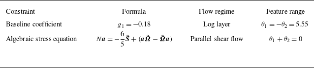
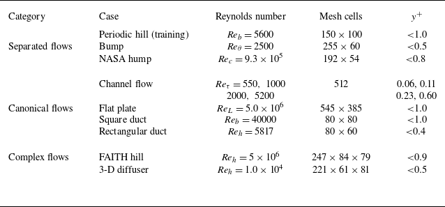

 Ux/Ub

 Ux
 Uy

 g1
 g1
 (θ1−θ1ℓ)2+(θ2+θ1ℓ)2=3σ1
 θ1+θ2=0

 Ux/Uref
 Ux/Uref
 Uy/Uref
 x/c

 Cf

 U+
 y+
 Reτ=550
 Reτ=1000
 Reτ=2000
 Reτ=5200
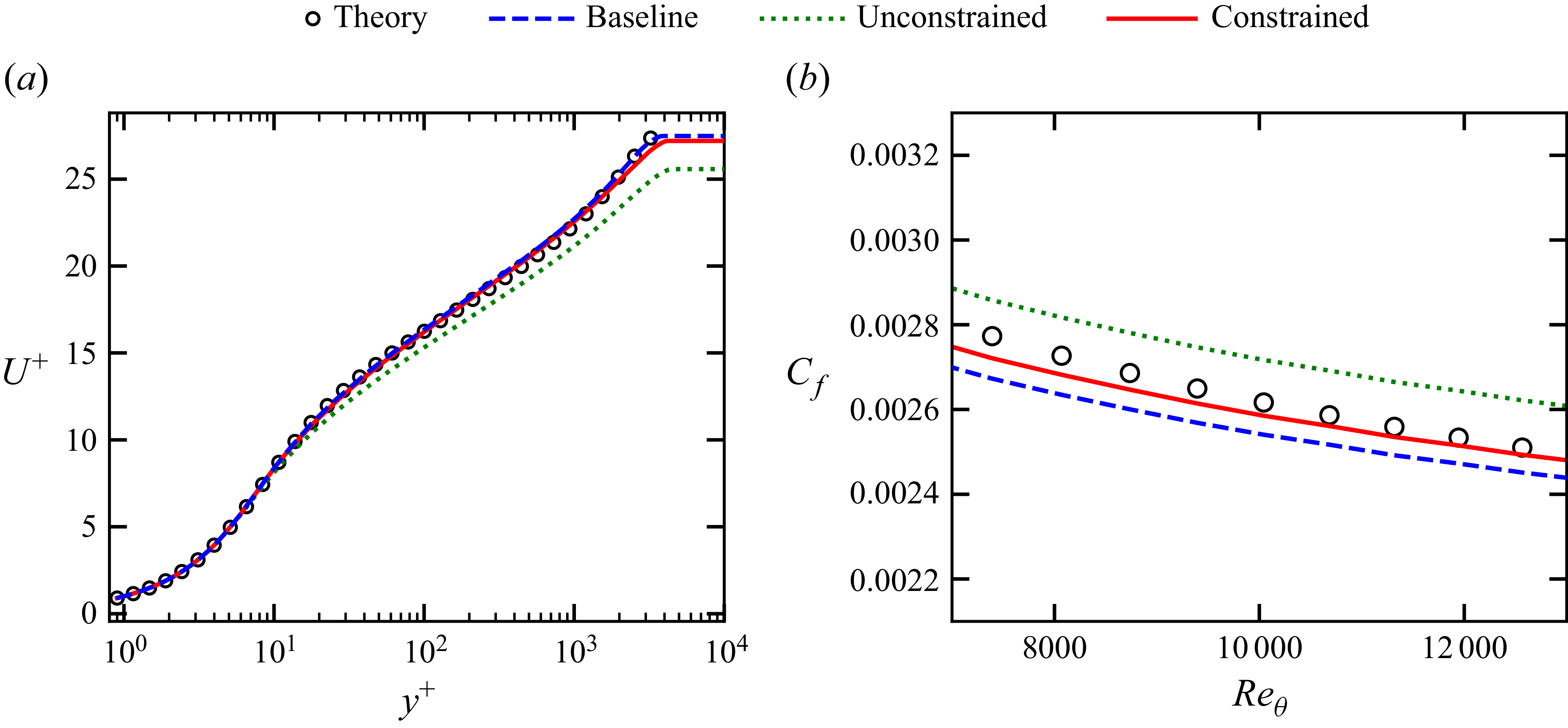
 U+
 y+
 Cf
 Reθ

 Ux/Ub
 Uy/Ub
 y/h
 z/h


 y/h
 z/h
 Reb=5817
 Ux/Ub
 Uy/Ub
 Uz/Ub
 Ub
 h

 AR=3
 z/h
 y/h


 U/U∞=0

 x/h=−9

 x/h=2,5,8,12, and 15
 y/h (wall-normal)
 z/h (spanwise)
 Ux/Ub
 Ux/Ub=0

 z/h=2.918
 y/h
 x/h
 z/h=2.918
 Ux/Ub=0
 x/h
 y/h
 z/h=2.918

 νt/ν

 g1
 g2
 θ1
 θ2
 −g1
 g1=−0.18
 θ1+θ2=0
 −g2

 y