



1. Introduction
Supersonic and hypersonic flight vehicles suffer significant wave drag during high-speed flight, which severely compromises aerodynamic performance. Energy deposition techniques generate a high-energy plasma region in the flow field via laser excitation, electrical discharge or microwaves (Padhi & Joarder Reference Padhi and Joarder2022). The resulting blast wave interacts with the vehicle’s bow shock, modifying the shock structure and flow field to achieve effective flow control. Specifically, nanosecond pulsed lasers offer high peak power density, facilitating air breakdown and plasma formation. Combined with advantages such as high directionality, controllability, airborne suitability and non-intrusiveness to the aerodynamic profile, they hold significant promise for active flow control, particularly in drag reduction applications.
Investigating the mechanisms of drag reduction via nanosecond pulsed laser energy deposition requires a numerical model capable of accurately representing the deposition evolution and associated flow characteristics. Ideally, such a model should reproduce the following phenomena (Han et al. Reference Han, Wang, Pu, Chen and Zheng2022): (i) the formation of the plasma region; (ii) the evolution of the thermal kernel and blast-wave propagation in quiescent air; and (iii) the interaction between the deposition-induced shock wave and the bow shock in supersonic flows. Consequently, current academic research has bifurcated into two primary modelling categories: cross-scale energy deposition models and instantaneous energy deposition models.
Cross-scale models aim to resolve the formation and deformation of high-temperature plasma with varying levels of physical detail. An early example is the work of Kandala & Candler (Reference Kandala and Candler2004), who developed a Nd:YAG laser energy deposition model for supersonic flow control. Their model included inverse-bremsstrahlung absorption, the evolution of the plasma shape and structure, air-breakdown chemistry and the subsequent fluid-dynamic response, and was applied to quiescent air, supersonic flow past a sphere, and Edney type-IV shock–shock interaction. More recently, Munafò et al. (Reference Munafò, Alberti, Pantano, Freund and Panesi2020) employed radiative-transfer equations, accounting for multiphoton ionization and inverse bremsstrahlung, to simulate nanosecond-scale laser–plasma interactions. Their model successfully reproduced the microscopic double-lobe structure observed during plasma formation within quiescent air. While such models can describe key aspects of the air-breakdown and laser–plasma-formation processes, they are computationally expensive and algorithmically complex. Their direct use for predicting the subsequent macroscopic blast-wave evolution and shock–shock interactions therefore remains demanding (Alberti et al. Reference Alberti, Munafò, Pantano and Panesi2021).
Given that the laser pulse width (typically
 ${\sim }10\,\text{ns}$
) is orders of magnitude shorter than the characteristic flow evolution time (
 $100{-}200$
μs), instantaneous energy deposition models are frequently adopted to reduce computational cost by neglecting the plasma generation phase. The first subcategory employs an energy source term in the energy equation, typically assuming a Gaussian spherical or ellipsoidal distribution (Zheltovodov et al. Reference Zheltovodov, Pimonov and Knight2007). Studies by Sakai et al. (Reference Sakai, Sekiya, Mori and Sasoh2008) and Yan & Gaitonde (Reference Yan and Gaitonde2008) have confirmed the reliability of this approach for predicting stagnation pressure variations and general flow features. However, these source-term models often fail to accurately capture the spatial distribution and morphological evolution of the plasma thermal kernel.
To capture the thermal-kernel evolution, initialization-based models were proposed, which patch a plasma seed with specific temperature, pressure and species distributions into the flow field. For example, Qing et al. (Reference Qing, Hong, Wang and Zhang2017), adapting the asymmetric teardrop model by Dors (Reference Dors2000), successfully predicted the three-lobe spike structure driven by the Richtmyer–Meshkov (RM) instability. However, these models typically rely on empirically prescribed temperature distributions that lack a rigorous thermodynamic link to the actual deposited energy, limiting their adaptability to varying energy conditions. Similarly, Wang et al. (Reference Wang, Buchta and Freund2020) utilized geometric parameterization with smooth transitions to simulate typical features such as the axial jet and vortex rings, yet the lack of direct energy coupling remains a critical unresolved issue.
Attempts to couple initialization parameters with the deposited energy have been made by Joarder et al. (Reference Joarder, Padhi, Singh and Tummalapalli2017), who determined the postdeposition composition and temperature using Helmholtz free-energy minimization under a local thermodynamic equilibrium (LTE) assumption. This work represents an important step towards thermodynamically informed initialization. However, the initialization problem was not formulated as a closed-loop procedure in which the spatially reconstructed kernel is subsequently checked against the prescribed absorbed energy. In addition, the use of a trapezoidal breakdown region may introduce sharp parameter transitions, and the required minimization procedure can be relatively involved for implementation.
To clarify the incremental advance of the present work, table 1 compares representative instantaneous energy-deposition (ED) modelling approaches in terms of asymmetric kernel morphology, energy coupling, field-level energy closure, field smoothness and thermochemical consistency. The comparison indicates that existing models usually emphasize only part of the overall modelling requirements, and a unified treatment that simultaneously ensures morphology-informed field construction, thermochemical consistency, smooth field distributions and quantitative consistency with the prescribed absorbed energy remains insufficiently developed.
Comparison of representative instantaneous ED modelling approaches.

Table 1. Long description
A table comparing different energy-deposition modeling approaches across five criteria. The table has six rows and five columns. The columns are labeled Asymmetric kernel morphology, Energy coupling, Field-level energy closure, Field smoothness, and Thermochemical consistency. The rows are labeled Source-term models, Dors (2000), Qing et al. (2017), Wang et al. (2020), Joarder et al. (2017), and Present method. Each cell contains a checkmark, triangle, or dash indicating the presence, partial presence, or absence of the respective criterion. Row 1: Source-term models, Asymmetric kernel morphology dash, Energy coupling checkmark, Field-level energy closure triangle, Field smoothness checkmark, Thermochemical consistency dash. Row 2: Dors (2000), Asymmetric kernel morphology checkmark, Energy coupling triangle, Field-level energy closure checkmark, Field smoothness triangle, Thermochemical consistency checkmark. Row 3: Qing et al. (2017), Asymmetric kernel morphology checkmark, Energy coupling triangle, Field-level energy closure checkmark, Field smoothness triangle, Thermochemical consistency triangle. Row 4: Wang et al. (2020), Asymmetric kernel morphology checkmark, Energy coupling triangle, Field-level energy closure triangle, Field smoothness checkmark, Thermochemical consistency dash. Row 5: Joarder et al. (2017), Asymmetric kernel morphology checkmark, Energy coupling checkmark, Field-level energy closure dash, Field smoothness dash, Thermochemical consistency checkmark. Row 6: Present method, Asymmetric kernel morphology checkmark, Energy coupling checkmark, Field-level energy closure checkmark, Field smoothness checkmark, Thermochemical consistency checkmark.
 $\checkmark$
, explicitly included;
 $\triangle$
, partially or implicitly included; –, not explicitly included. ‘Energy coupling’ denotes whether the model input is directly related to the prescribed absorbed energy. ‘Field-level energy closure’ denotes whether the spatial field used to represent the deposited-energy region is checked by integrating the internal-energy increment against the prescribed absorbed energy.
To address these challenges, especially the disconnect between plasma seeds and deposited energy, the lack of smooth reconstructed fields and the algorithmic complexity of determining postdeposition parameters, this paper proposes a self-consistent modelling methodology for instantaneous energy deposition. The method couples thermochemical equilibrium calculations, energy conservation and experimentally informed kernel geometry in a closed-loop framework, such that the reconstructed spatial field is explicitly constrained by the prescribed absorbed energy. The methodology is validated against experiments in both quiescent air and supersonic flow over a blunt body. In addition, parameter sensitivity analyses are performed for the absorbed energy and key geometric parameters of the initialized thermal kernel. Consequently, this work provides both a reproducible initialization methodology for instantaneous energy deposition and a framework for connecting deposition parameters with shock, jet and vortex dynamics.
2. Establishment of the self-consistent energy deposition model
This section presents the proposed self-consistent methodology for initializing instantaneous energy deposition in numerical simulations. The objective is to construct an initial postdeposition flow field that is thermodynamically consistent with the prescribed absorbed energy. In the present framework, the initialization procedure is decomposed into two coupled parts: determination of the average postdeposition equilibrium state in the focal volume, and reconstruction of the corresponding spatial fields subject to a field-level energy-closure constraint. Figure 1 summarizes the overall workflow of the proposed initialization methodology.
Workflow of the self-consistent initialization methodology for instantaneous energy deposition.

2.1. General mathematical formulation of the thermal kernel initialization
For clarity, the initialization problem for the thermal kernel is formulated in a general form as a two-level coupled system.
Let
 $V_0$
denote the prescribed focal volume for energy deposition, and let
 $E_{\textit{abs}}$
be the absorbed energy. The ambient initial state is specified by
 $(\rho _0,T_{\textit{env}},p_{\textit{env}})$
, together with the initial composition of the gas mixture. The general chemical model is described by a species set
 $\mathcal{S}$
and a set of independent equilibrium reactions
 $\mathcal{R}$
,
 \begin{equation} \mathcal{S} = \{\mathcal{S}_1, \mathcal{S}_2, \ldots, \mathcal{S}_{N_s}\}, \qquad \mathcal{R} = \{\mathcal{R}_1, \mathcal{R}_2, \ldots, \mathcal{R}_{N_r}\}, \end{equation}
where
 $N_s$
and
 $N_r$
denote the numbers of species and independent equilibrium reactions, respectively.
The average postdeposition state in the focal volume is then described by
 \begin{equation} \boldsymbol{{q}}_{{ave}} = \left [ \sigma _1, \sigma _2, \ldots, \sigma _{N_s}, T_{{ave}}, p_{{ave}} \right ]^{\textit{T}}, \end{equation}
where
 $\sigma _i$
denotes the specific mole number of species
 $S_i$
, while
 $T_{{ave}}$
and
 $p_{{ave}}$
are the average temperature and pressure in the deposition region.
At the first level, the average state is obtained by solving a nonlinear algebraic system consisting of
 $N_s+2$
equations for
 $N_s+2$
unknowns,
 \begin{equation} \boldsymbol{F} \left ( \boldsymbol{{q}}_{{ave}}; E_{\textit{abs}}, V_0, \rho _0, T_{\textit{env}}, p_{\textit{env}} \right ) = \boldsymbol{0}, \end{equation}
where the unknown vector is
 $\boldsymbol{{q}}_{{ave}} \in \mathbb{R}^{N_s+2}$
. In general, the system is composed of elemental conservation equations, charge-neutrality constraints if ionized species are included,
 $N_r$
independent equilibrium relations, one global energy-conservation equation and one constant-volume constraint. Accordingly, the first-level problem determines the unknown species composition, temperature and pressure under the combined constraints of chemistry, conservation laws and thermodynamics.
At the second level, the local thermodynamic fields are reconstructed from the average state. The temperature field is introduced in the general form
 \begin{equation} T = T(\boldsymbol{{x}}; \boldsymbol{{\lambda }}), \end{equation}
where
 $\boldsymbol{{x}}$
is the spatial coordinate and
 $\boldsymbol{{\lambda }}$
denotes a set of reconstruction parameters. Once the temperature field has been specified, the local species composition and pressure fields are determined as
 \begin{equation} \begin{aligned} Y_i &= Y_i(T; p_{{ave}}, \mathcal{S}, \mathcal{R}), \\ p &= p(\boldsymbol{{x}}; T, Y_i), \end{aligned} \end{equation}
through the equilibrium relations (Pimentel & Jr Reference Pimentel and Jr2011) and the equation of state. Here,
 $Y_i$
denotes the mass fraction of species
 $i$
. When required by the thermodynamic relations or the equation of state, it can be equivalently converted to the specific mole number as
 $\sigma _i=Y_i/M_i$
, where
 $M_i$
is the molar mass of species
 $i$
. The reconstruction parameters
 $\boldsymbol{{\lambda }}$
are then determined from a field-level energy-closure condition,
 \begin{equation} \mathcal{G}(\boldsymbol{{\lambda }}) = \int _{\varOmega } \left ( E_{\textit{after}} - E_{\textit{before}} \right ) \, \mathrm{d}\varOmega - E_{\textit{abs}} = 0, \end{equation}
so that the spatially integrated internal-energy increment exactly matches the prescribed absorbed energy.
The present initialization methodology is established under an instantaneous LTE assumption for the postdeposition kernel, such that a single temperature is used to characterize the thermodynamic state immediately after deposition. This assumption is commonly adopted in existing instantaneous ED models, and it provides a practical thermodynamic closure for the initialization problem considered here. At the same time, it remains an idealization. In particular, under lower-pressure or higher-enthalpy conditions, the relaxation of internal energy modes may not be sufficiently rapid for a single-temperature LTE description to remain strictly valid. The possible limitations associated with this assumption therefore deserve further assessment, and extending the present framework beyond the LTE approximation will be investigated in future work.
In the present work, this general formulation is instantiated using a seven-species air model for the equilibrium calculation and a representative teardrop-shaped distribution for the field reconstruction. These specific implementations are described in §§ 2.2 and 2.3, respectively.
2.2. Thermochemical equilibrium analysis for the present seven-species model
This subsection instantiates the first-level problem introduced in § 2.1 for the present seven-species air model. Specifically, the general species set
 $ \mathcal{S}$
, the reaction set
 $ \mathcal{R}$
and the average-state vector
 $ \boldsymbol{q}_{{ave}}$
are here specified for the equilibrium calculation adopted in the subsequent simulations. The initial air composition is assumed to be 79 %
 $\mathrm{N}_2$
and 21 %
 $\mathrm{O}_2$
by volume, with an initial density of
 $\rho _0$
. Upon cessation of the laser pulse, the thermal kernel is represented by a focal volume
 $V_0$
with uniform temperature, pressure and species distributions. To remain consistent with the subsequent chemically reacting flow simulation, the chemical model adopted here contains the same seven species as in Park’s air chemistry, namely
 $\mathrm{N}_2$
,
 $\mathrm{O}_2$
,
 $\mathrm{N}$
,
 $\mathrm{O}$
,
 $\mathrm{NO}$
,
 $\mathrm{NO}^+$
and
 $\mathrm{e}^-$
. The absorbed laser energy is denoted by
 $E_{\text{abs}}$
.
For this specific model, the general nonlinear system in (2.3) reduces to a closed system of nine equations for nine unknowns, namely the average temperature
 $ T_{{ave}}$
, the average pressure
 $ p_{{ave}}$
and the specific moles
 $ \sigma _i$
of the seven species. These equations comprise atomic mass conservation, charge neutrality, independent chemical-equilibrium relations, energy conservation and the constant-volume constraint.
The global chemical reaction equation governing the plasma region is expressed as
 \begin{equation} n_{{\rm N}_2}^{\textit{react}} {\rm N}_2 + n_{{\rm O}_2}^{\textit{react}} {\rm O}_2 \rightleftharpoons n_{{\rm N}_2}^{\textit{prod}} {\rm N}_2 + n_{{\rm O}_2}^{\textit{prod}} {\rm O}_2 + n_{{\rm NO}}^{\textit{prod}} {\rm NO} + n_{\rm N}^{\textit{prod}} N + n_{\rm O} ^{\textit{prod}} {\rm O} + n_{{\rm NO}^+}^{\textit{prod}} {\rm NO}^+ + n_{e^-}^{\textit{prod}} e^{-}, \end{equation}
where
 $ n_i^{\textit{react}}$
and
 $ n_i^{\textit{prod}}$
are the initial (reactant) and final (product) moles of species
 $ i$
, respectively.
Mass conservation for nitrogen and oxygen atoms gives
 \begin{equation} \begin{aligned} N &\Rightarrow 2n_{{\rm N}_2}^{\textit{react}} = 2n_{{\rm N}_2}^{\textit{prod}} + n_{\rm N}^{\textit{prod}} + n_{{\rm NO}}^{\textit{prod}} + n_{{\rm NO}^+}^{\textit{prod}}, \\ {\rm O} &\Rightarrow 2n_{{\rm O}_2}^{\textit{react}} = 2n_{{\rm O}_2}^{\textit{prod}} + n_{\rm O} ^{\textit{prod}} + n_{{\rm NO}}^{\textit{prod}} + n_{{\rm NO}^+}^{\textit{prod}}. \end{aligned} \end{equation}
Expressed in terms of mole numbers per unit mass, the mass balance equations become
 \begin{equation} \begin{aligned} 2\sigma _{{\rm N}_2}^0 &= 2\sigma _{{\rm N}_2} + \sigma _{\rm N} + \sigma _{{\rm NO}} + \sigma _{{\rm NO}^+}, \\ 2\sigma _{{\rm O}_2}^0 &= 2\sigma _{{\rm O}_2} + \sigma _{\rm O} + \sigma _{{\rm NO}} + \sigma _{{\rm NO}^+},\end{aligned} \end{equation}
where
 $ \sigma _{{\rm N}_2}^0$
and
 $ \sigma _{{\rm O}_2}^0$
are the initial specific moles of
 $\mathrm{N}_2$
and
 $\mathrm{O}_2$
, respectively.
Furthermore, the assumption of charge neutrality (charge conservation) imposes
 \begin{equation} \sigma _{{\rm NO}^+} = \sigma _{e^-}. \end{equation}
According to the thermodynamic equilibrium constant method (Pimentel & Jr Reference Pimentel and Jr2011), the equilibrium composition at a given temperature and pressure can be determined from the equilibrium constants of independent reactions. For the present seven-species model, the following four independent reactions are introduced:
 \begin{equation} \begin{aligned} &\text{N}_2 \rightleftharpoons 2\text{N}, \\ &\text{O}_2 \rightleftharpoons 2\text{O}, \\ &\text{N}_2 + \text{O}_2 \rightleftharpoons 2\text{NO}, \\ &\text{NO}^+ + \text{e}^- \rightleftharpoons \text{NO}. \end{aligned} \end{equation}
The corresponding equilibrium relations are
 \begin{equation} \begin{aligned} &K_1 \sigma _{{\rm N}_2} - \rho \sigma _{\rm N}^2 = 0, \\ &K_2 \sigma _{{\rm O}_2} - \rho \sigma _{\rm O} ^2 = 0, \\ &K_3 \sigma _{{\rm N}_2} \sigma _{{\rm O}_2} - \sigma _{{\rm NO}}^2 = 0, \\ &\rho K_4 \sigma _{{\rm NO}^+} \sigma _{e^-} - \sigma _{{\rm NO}} = 0, \end{aligned} \end{equation}
where the equilibrium constants are calculated from
 \begin{equation} \begin{aligned} &K_{\!j} = K_{p,j} (p_{\textit{ref}} / R_uT)^{\Delta N}, \\ &K_{p,j} = \exp \big [-\Delta G_{\!j}^{\theta } / (R_uT)\big ] .\end{aligned} \end{equation}
Here,
 $ p_{\textit{ref}}$
is the standard state pressure,
 $ R_u$
is the universal gas constant and
 \begin{equation} \begin{aligned} &\Delta N = \sum _i \nu _i^{\textit{prod}} - \sum _i \nu _i^{\textit{react}},\\ &\Delta G_{\!j}^{\theta } = \sum _i \nu _i^{\textit{prod}} G_i - \sum _i \nu _i^{\textit{react}} G_i,\end{aligned} \end{equation}
with
 $ \nu _i$
denoting the stoichiometric coefficient of species
 $ i$
. For the four reactions in (2.11), the values of
 $ \Delta N$
are 1, 1, 0 and −1, respectively.
Because the present problem is posed for a prescribed absorbed energy, both temperature and pressure are unknown and must be solved simultaneously together with the species composition. Two additional closure equations are therefore introduced through energy conservation and the constant-volume constraint. Global energy conservation yields
 \begin{equation} U_0 + \frac {E_{\textit{abs}}}{\rho _0 V_0} = \sum _{i=1}^{7} U_i(T_{{ave}}), \end{equation}
where
 $ U_0$
is the initial specific internal energy (per unit mass) composed of species
 $\mathrm{N}_2$
and
 $\mathrm{O}_2$
, and
 $ U_i$
is the specific internal energy of species
 $ i$
in the focal region after energy deposition. These quantities are expressed as
 \begin{equation} \begin{aligned} U_0 &= \sigma _{{\rm N}_2}^{0}(H_{{\rm N}_2} - R_uT_{\textit{env}}) + \sigma _{{\rm O}_2}^{0}(H_{{\rm O}_2} - R_uT_{\textit{env}}), \\ U_i &= \sigma _i (H_i - R_uT_{{ave}}) .\end{aligned} \end{equation}
Assuming that the focal volume remains constant before and after deposition, the equation of state gives
 \begin{equation} \frac {\rho _0 V_0}{\rho } = \frac {\sum _{i=1}^{7}\sigma _i \rho _0 V_0 R_u T_{{ave}}}{p_{{ave}}} = V_0. \end{equation}
Accordingly, the average postdeposition state is determined by solving the following nonlinear algebraic system:
 \begin{equation} \begin{aligned} &f_1(\sigma _i, T_{{ave}}, p_{{ave}}) = 2\sigma _{{\rm N}_2} + \sigma _{\rm N} + \sigma _{{\rm NO}} + \sigma _{{\rm NO}^+} - 2\sigma _{{\rm N}_2}^0 = 0, \\[7pt] &f_2(\sigma _i, T_{{ave}}, p_{{ave}}) = 2\sigma _{{\rm O}_2} + \sigma _{\rm O} + \sigma _{{\rm NO}} + \sigma _{{\rm NO}^+} - 2\sigma _{{\rm O}_2}^0 = 0, \\[7pt] &f_3(\sigma _i, T_{{ave}}, p_{{ave}}) = \sigma _{{\rm NO}^+} - \sigma _{e^-} = 0, \\[7pt] &f_4(\sigma _i, T_{{ave}}, p_{{ave}}) = K_1 \sigma _{{\rm N}_2} - \rho \sigma _{\rm N}^2 = 0, \\[7pt] &f_5(\sigma _i, T_{{ave}}, p_{{ave}}) = K_2 \sigma _{{\rm O}_2} - \rho \sigma, \\[7pt]&f_6(\sigma _i, T_{{ave}}, p_{{ave}}) = K_3 \sigma _{{\rm N}_2} \sigma _{{\rm O}_2} - \sigma^{2}_{\rm NO} = 0, \\[7pt]&f_7(\sigma _i, T_{{ave}}, p_{{ave}}) = \rho K_4 \sigma _{{\rm NO}^{+}} \sigma _{e^{-}} - \sigma_{\rm NO} = 0, \\[7pt]&f_8(\sigma _i, T_{{ave}}, p_{{ave}}) = U_0 + E_{\textit{abs}} / (\rho_0 V_0) - \sum_{i=1}^7 U_{i} = 0 \\&f_9(\sigma _i, T_{{ave}}, p_{{ave}}) = \sum_{i=1}^7 \sigma _{i} \rho_0 R_u T_{{ave}} - p_{{ave}} =0 \end{aligned}\end{equation}
where the mixture density
 $ \rho$
can be expressed in terms of the unknowns via
 \begin{equation} \rho = \frac {p_{{ave}}}{\sum _{i=1}^{7}\sigma _i R_u T_{{ave}}}. \end{equation}
The thermodynamic properties required in the above formulation, including the evaluations of
 $H_i$
,
 $S_i$
and
 $G_i$
, are summarized in Appendix A. This arrangement keeps the main derivation focused on the structure of the equilibrium problem while retaining the information necessary for reproducibility.
The proposed model is validated by comparing its predictions for the average postdeposition state with NASA CEA (chemical equilibrium with applications) software. The initial conditions are
 $ T_{\textit{env}} = 300\,\mathrm{K}$
,
 $ p_{\textit{env}} = 101\,325\,\mathrm{Pa}$
,
 $ \rho _0 = 1.172\,\mathrm{kg\,m}^{-3}$
and the focal volume
 $ V_0 = 3 \times 10^{-9}\,\mathrm{m}^3$
. The NASA-CEA software is run in constant-internal-energy and constant-volume mode using the same initial internal energy plus absorbed energy
 $ E_{\textit{abs}}$
. The comparison is presented in table 2. The close agreement between the two sets of data validates the proposed thermochemical equilibrium calculation. Furthermore, the predicted electron density for the
 $ 100\,\mathrm{mJ}$
case is of the order of
 $ 10^{22}\,\mathrm{m}^{-3}$
, which matches well with experimental observations reported by Fukui et al. (Reference Fukui, Kawamura, Komurasaki, Koizumi and Arakawa2007) and Gautam & Parigger (Reference Gautam and Parigger2017) under comparable conditions. Therefore, the present method provides an alternative convenient and efficient approach for resolving thermochemical equilibrium states of the thermal kernel, which then serves as the input to the spatial reconstruction procedure in § 2.3.
Comparison of postdeposition equilibrium parameters calculated by the proposed method versus NASA-CEA.

Table 2. Long description
A table comparing postdeposition equilibrium parameters calculated by the proposed method versus NASA-CEA. The table has 10 rows and 6 columns. The columns are labeled as Method, This paper, NASA-CEA, This paper, NASA-CEA, This paper, and NASA-CEA. The rows are labeled with different parameters: E_abs (mJ), T_ave (K), p_ave (bar), X_N2, X_O2, X_N, X_O, X_NO, X_NO+, and X_e-. Each row provides values for these parameters calculated by the proposed method and NASA-CEA. The table shows the comparison for three different values of E_abs: 10 mJ, 50 mJ, and 100 mJ.
2.3. Spatial reconstruction and energy closure for the present kernel configuration
This subsection instantiates the second-level problem introduced in § 2.1. Using the average equilibrium state
 $(\sigma _i, T_{{ave}}, p_{{ave}})$
obtained in § 2.2, the general temperature field
 $ T(\boldsymbol{x}; \boldsymbol{\lambda })$
is specified using a representative analytical kernel distribution, and the reconstruction coefficient is determined from the energy-closure condition
 $ \mathcal{G}(\boldsymbol{\lambda }) = 0$
. To illustrate the procedure in a concrete manner, the
 $100\,\mathrm{mJ}$
case is used here as an example.
First, the spatial temperature distribution is defined based on a typical teardrop shape summarized from experimental observations (Dors Reference Dors2000), while acknowledging that the exact morphology may vary with laser and focusing conditions. Taking the centre of energy deposition as the origin, with the laser incident direction from right to left, the temperature distribution within the
 $ xy$
plane of the axisymmetric model after the pulse energy deposition ceases satisfies
 \begin{align} T_c(x,y) = k T_{{ave}} \exp (-\beta _x x) \exp \left [ -\left ( \frac {y}{W_0 \exp (\beta _r x)} \right )^2 \right ]\!, \quad -L_0 \le x \le L_0, \end{align}
where
 $\beta _x$
,
 $\beta _r$
,
 $W_0$
and
 $L_0$
are geometric parameters describing the kernel shape, and
 $k$
is a reconstruction coefficient determined from the energy-closure condition. The numerical values of these geometric parameters are given in Appendix B. The quantity
 $T_{{ave}}$
is the average equilibrium temperature obtained from § 2.2; for the present
 $100\,\mathrm{mJ}$
case,
 $T_{{ave}}=9392.42\,\mathrm{K}$
according to table 2.
The core profile in (2.20) follows an exponential variation along the laser axis and a Gaussian variation in the transverse direction. To ensure a smooth transition at both ends of the thermal kernel, Gaussian ellipsoidal extensions are appended to the left- and right-hand sides
 \begin{equation} \begin{aligned} T_L(x,y) &= T_L^C \exp \left [ -\left ( \left ( \frac {x - x_L}{R_a^L} \right )^2 + \left ( \frac {y - y_L}{R_b^L} \right )^2 \right ) \right ]\!, \quad x \lt -L_0,\\ T_R(x,y) &= T_R^C \exp \left [ -\left ( \left ( \frac {x - x_R}{R_a^R} \right )^2 + \left ( \frac {y - y_R}{R_b^R} \right )^2 \right ) \right ]\!, \quad x \gt L_0, \end{aligned} \end{equation}
where
 $(x_L,y_L)=(-L_0,0)$
and
 $(x_R,y_R)=(L_0,0)$
, while
 $R_a^L$
,
 $R_b^L$
,
 $R_a^R$
and
 $R_b^R$
denote the semiaxes of the two appended ellipsoidal lobes. The amplitudes
 $T_L^C=T_c(x_L,y_L)$
and
 $T_R^C=T_c(x_R,y_R)$
are chosen to ensure continuity between the central and side distributions. The numerical values of all geometric parameters are listed in Appendix B.
An alternative smoothing uses exponential decay
 \begin{equation} T_{L,R}(x,y) = T_{L,R}^C \exp (-\alpha \times |x - x_{L,R}|), \end{equation}
where the coefficient
 $ \alpha$
is the decay constant, taken as
 $ 1.6\times 10^{4}\,\mathrm{m}^{-1}$
here. In the present work, both treatments produce nearly identical temperature fields, whereas the Gaussian-ellipsoidal smoothing is retained because of its better smoothness. Temperatures below the ambient value are clipped to
 $T_{\textit{env}}$
. Figure 2 shows the reconstructed two-dimensional temperature field for the
 $100\,\mathrm{mJ}$
case. In three-dimensional calculations, this two-dimensional profile is revolved around the laser axis.
Initial temperature distributions of the thermal kernel: (
 $a$
) Gaussian-ellipsoidal smoothing; (
 $b$
) exponential-decay smoothing.

Next, the local species distributions are reconstructed from the equilibrium composition as a function of temperature under the constant average pressure
 $p_{{ave}}$
. Specifically, (2.7)–(2.12) are solved over a temperature range at fixed
 $p_{{ave}}$
, yielding the equilibrium mass-fraction functions
 $Y_i(T)$
. For the
 $100\,\mathrm{mJ}$
example, the resulting temperature-dependent mass fraction and mole fraction are shown in figure 3. The local species mass fractions are then assigned by mapping the reconstructed local temperature field
 $T(x,y)$
to these equilibrium functions, as expressed by
 \begin{equation} Y_i(x,y)=Y_i\!\left (T(x,y)\right )\!. \end{equation}
Mass fraction and mole fraction of seven species as a function of temperature at constant pressure.

The resulting field distributions of the seven species are presented in figure 4(
 $a$
–
 $g$
). Together with the pressure field obtained below, they constitute the thermochemical initial condition supplied to the flow solver. The pressure distribution is then obtained from the reconstructed temperature and composition fields through the equation of state
 \begin{equation} p(x,y) = \rho _0 R_u T(x,y) \sum _{i=1}^{7}\sigma _i(x,y) = \rho _0 R_u T(x,y) \sum _{i=1}^{7}\frac {Y_i(x,y)}{M_i}. \end{equation}
Here, the density is taken as
 $\rho _0$
at this initialization stage, consistent with the constant-volume assumption. The resulting pressure field is shown in figure 4(
 $h$
).
Reconstructed thermochemical fields for the representative
 $100\,\mathrm{mJ}$
case: (
 $a$
–
 $g$
) mass-fraction distributions of the seven species; (
 $h$
) pressure distribution.

Finally, the scaling coefficient
 $ k$
in (2.20) is determined from the field-level energy-closure condition. In practice,
 $k$
is adjusted iteratively until the spatial integral of the internal-energy increment equals the prescribed absorbed energy,
 \begin{align} E_{\textit{ed}} &= 2\pi \int _{x=-1\,\mathrm{mm}}^{1\,\mathrm{mm}} \int _{y=0\,\mathrm{mm}}^{1\,\mathrm{mm}} \left (E_{\textit{after}}-E_{\textit{before}}\right ) y\,\mathrm{d}y\,\mathrm{d}x \end{align}
where
 \begin{equation} \begin{aligned} &E_{\textit{after}} = \rho \sum (U_i)_{T = T(x,y)} = \sum (\rho _0 H_i \sigma _i)_{T = T(x,y)} - p(x,y), \\ &E_{\textit{before}} = \rho _0 (U_0)_{T = T_{\textit{env}}} = \sum (\rho _0 H_i \sigma _i)_{T = T_{\textit{env}}} - p_{\textit{env}}. \end{aligned} \end{equation}
Therefore, the final initialized field is obtained after the reconstruction coefficient
 $ k$
has been determined from the energy-closure condition. For the
 $100\,\mathrm{mJ}$
example, the converged value is
 $k=2.56$
, yielding an integrated absorbed energy of
 $100.12\,\mathrm{mJ}$
, which demonstrates good agreement with the prescribed input. In this way, the reconstructed kernel is not merely geometrically plausible, but also strictly consistent with the specified absorbed energy. This closes the second-level problem defined in § 2.1.
3. Improved solver for energy deposition
The hydrodynamic evolution following energy deposition is characterized by localized, asymmetric region of high temperature and pressure. Resolving the subsequent multiscale evolution of the thermal kernel, particularly the RM-type instability arising from misaligned pressure and density gradients, demands a numerical scheme of high fidelity and robustness. In the present work, the open-source solver hy2Foam (Casseau et al. Reference Casseau, Espinoza, Scanlon and Brown2016a , Reference Casseau, Palharini, Scanlon and Brownb ) is adopted as the baseline framework. This solver was originally developed from rhoCentralFoam and extended for thermochemical non-equilibrium applications. Although the standard density-based solver effectively captures shock positions and interactions, preliminary simulations reveal its inadequacy in resolving the finescale morphological evolution of the thermal kernel. This deficiency primarily stems from excessive numerical diffusion near contact discontinuities. To address this issue, advanced reconstruction strategies from HiSA (high-speed aerodynamic solver) (Heyns et al. Reference Heyns, Oxtoby and Steenkamp2014; Abuhanieh et al. Reference Abuhanieh, Bicer and Sahin2021) were incorporated into the hy2Foam together with a series of targeted algorithmic modifications, resulting in the improved solver hisa2Foam.
3.1. Algorithmic modifications
In a finite-volume framework, numerical fluxes across cell faces are used to update cell-averaged quantities. To achieve second-order or higher spatial accuracy, face values must be reconstructed from cell-centre data. The monotone upstream-centred schemes for conservation laws (MUSCL) method approximates the variable distribution within a cell using a linear or higher-order polynomial. For a cell
 $C$
with centre value
 $\phi _{C}$
and gradient
 $(\boldsymbol{\nabla }\phi )_{C}$
, an unlimited linear reconstruction at its face
 $F$
shared with neighbour cell
 $N$
is
 \begin{equation} \phi _{F,\textit{unlimited}} = \phi _{C} + (\boldsymbol{r}_{F} - \boldsymbol{r}_{C})\boldsymbol{\cdot }(\boldsymbol{\nabla }\phi )_{C}, \end{equation}
where
 $\boldsymbol{r}$
denotes the position vector. To prevent non-physical numerical oscillations near discontinuities, a slope limiter
 $\psi \in [0,1]$
is introduced, giving
 \begin{equation} \phi _{F} = \phi _{C} + \psi \left [(\boldsymbol{r}_{F} - \boldsymbol{r}_{C})\boldsymbol{\cdot }(\boldsymbol{\nabla }\phi )_{C}\right ]\!. \end{equation}
The limiter
 $\psi = f(r)$
depends on a smoothness indicator
 $r$
, often defined using upstream, central, and downstream cells. A typical gradient-based formulation is
 \begin{equation} r = \frac {2(\boldsymbol{\nabla }\phi )_{C}\boldsymbol{\cdot }(\boldsymbol{r}_{N} - \boldsymbol{r}_{C})}{(\phi _{N} - \phi _{C})} - 1. \end{equation}
Based on this general reconstruction framework, four targeted modifications were introduced for localized high-enthalpy flow simulations: an AUSM
 $^+$
-up flux scheme, componentwise slope limiting, primitive-variable reconstruction and a geometry-aware weighted limiter.
3.1.1. Low-dissipation flux scheme
The Kurganov scheme used in the original hy2Foam solver is robust, but it introduces appreciable numerical diffusion when applied to the sharp gradients generated by localized energy deposition. To improve interface resolution, the AUSM
 $^+$
-up flux scheme (Liou Reference Liou2006) was implemented as an alternative convective-flux scheme. This scheme provides a more favourable balance between shock-capturing robustness and low numerical dissipation, which is essential for preserving the blast-wave structure and the steep density gradients around the thermal kernel.
3.1.2. Componentwise slope limiting
For vector or tensor fields
 $\varPhi$
(e.g. velocity
 $\boldsymbol{U}$
), traditional uniform limiting strategies compute a single scalar limiter
 $\psi _{\textit{scalar}}$
from a proxy field (e.g.
 $\phi _{\textit{scalar}} = f(\varPhi ) = \boldsymbol{U}\boldsymbol{\cdot }\boldsymbol{U}$
) and apply it indiscriminately to all components of
 $\varPhi$
. While this method preserves the reconstruction direction, it introduces unnecessary numerical dissipation to certain components when different components exhibit disparate smoothness. The implemented componentwise limiting method calculates and applies independent limiters
 $\psi _{k}$
for each component
 $\phi _{k}$
based on its own smoothness indicator
 $r_{k}$
:
 \begin{equation} \left (\phi _{F}\right )_{k} = \left (\phi _{C}\right )_{k} + \psi _{k}\left [(\boldsymbol{r}_{F} - \boldsymbol{r}_{C})\boldsymbol{\cdot }(\boldsymbol{\nabla }\phi _{C})_{k}\right ]\!. \end{equation}
This componentwise treatment avoids over-limiting relatively smooth components while retaining monotonicity near discontinuities. And the modification is particularly important for maintaining the initial kernel morphology that later drives the development of the RM-type instability.
3.1.3. Primitive-variable reconstruction
To further improve the fidelity of the solver and reduce reconstruction-induced distortion, the interpolation procedure was reformulated in terms of primitive variables rather than conservative variables. Since pressure, temperature and velocity are more directly related to the local physical state, reconstructing primitive variables improves numerical behaviour in regions of strong thermodynamic gradients.
3.1.4. Geometry-aware weighted slope limiter
A geometry-aware weighted limiting treatment was introduced to improve reconstruction quality on stretched or non-orthogonal meshes. In this approach, the limiter is modified according to the local face-flux direction, so that the limiter remains appropriately biased towards the upwind or downwind side depending on the local flow direction. To illustrate this modification, the classical van Leer limiter is taken as the reference form and then rewritten by incorporating a direction-dependent weighting coefficient. The resulting weighted van Leer (wvanLeer) limiter is expressed as
 \begin{equation} \psi _{\textit{new}}= \left \{ \begin{array}{ll} \dfrac {r+r^2}{2r+\mathrm{cd}(1-r)^2}, & \mathrm{if}\quad r\gt 0,\\[12pt] 0, & \mathrm{otherwise}, \end{array} \right . \end{equation}
followed by the final bounded form
 \begin{equation} \psi _{\textit{final}}= \max \left ( \min \left ( \min \left (\dfrac {r}{\mathrm{cd}},\psi _{\textit{new}}\right )\!,\dfrac {1}{\mathrm{cd}} \right )\!,0 \right )\!. \end{equation}
This treatment preserves the designed second-order accuracy while maintaining monotonicity and improving robustness on highly stretched or distorted grids.
With these modifications, the improved hisa2Foam solver provides a substantially better numerical basis for simulating localized ED flows than the original hy2Foam solver. A supplementary simplified benchmark was used to isolate the numerical behaviour of the solver from thermochemical effects and to compare different flux and limiter combinations. For conciseness, the detailed set-up and comparative results are presented in Appendix C. The benchmark results show that the improved solver preserves the thermal-kernel interface and the associated pressure and density gradients much more effectively than the baseline solver, thereby providing the numerical foundation for the physically complete validation cases discussed in § 4.
4. Results and discussion
4.1. Validation of energy deposition methodology
To comprehensively validate the self-consistent energy deposition methodology, this study conducts comparative benchmarks with experiments in both quiescent air and supersonic flow over a blunt body. The same geometric kernel shape is used in all validation cases considered in this paper. The corresponding geometric parameters are listed in Appendix B. Therefore, table 3 focuses on the case-dependent thermodynamic quantities, including the absorbed energy, ambient state, average postdeposition equilibrium state, species composition and reconstruction coefficient
 $k$
. Together with the geometric parameters in Appendix B, these quantities fully define the initialized ED field. The tabulated data indicate that low-pressure and low-temperature environments produce a more pronounced temperature rise and stronger ionization within the deposition region under the same deposited energy, owing to their lower gas density and smaller energy storage capacity. A small discrete energy-closure correction is applied to the deposition coefficient
 $k$
after the reconstructed fields are projected onto the finite-volume mesh. This correction compensates for the slight energy discrepancy introduced by finite grid resolution, cell-centred initialization and truncation of the localized kernel profile, ensuring that the initialized numerical field contains the prescribed absorbed energy.
Thermodynamic and energy-closure parameters for validation cases of single-pulse laser energy deposition. The same geometric kernel parameters are used for all cases and are listed in Appendix B.

Table 3. Long description
A table comparing thermodynamic and energy-closure parameters for different cases of single-pulse laser energy deposition. The table has three columns: Case, ED in quiescent air, and ED in supersonic flow. It contains data for various parameters including absorbed energy, ambient state, average postdeposition equilibrium state, species composition, and reconstruction coefficient. The table has 12 rows and 3 columns. Row 1: E_abs (mJ), 10, 72, 8.0. Row 2: T_env (K), 283, 283, 163. Row 3: p_env (Pa), 101301, 101301, 13800. Row 4: T_ave (K), 2951.9, 8196.6, 5541.76. Row 5: p_ave (bar), 10.63, 42.37, 5.68. Row 6: X_N2, 0.763042, 0.371233, 0.621478. Row 7: X_O2, 0.180358, 0.000373, 0.003279. Row 8: X_N, 0.000003, 0.337644, 0.034624. Row 9: X_O, 0.012790, 0.276109, 0.312342. Row 10: X_NO, 0.043807, 0.013315, 0.028139. Row 11: X_NO+, 0, 0.000663, 0.000069. Row 12: X_e-, 0, 0.000663, 0.000069. Row 13: n_e- (m^-3), -, 2.48 x 10^22, 5.09 x 10^20. Row 14: k, 1.82, 2.03, 1.78.
The model assumes the thermal kernel reaches LTE instantaneously upon the cessation of the laser pulse (Joarder et al. Reference Joarder, Padhi, Singh and Tummalapalli2017). This LTE assumption allows the state of the thermal kernel to be characterized by a single temperature, significantly simplifying the energy equations by avoiding separate conservation equations for different internal energy modes. The postdeposition kernel evolution is simulated as an axisymmetric, unsteady, compressible laminar reacting flow. Thermodynamic non-equilibrium effects are neglected, as the validation cases fall outside the hypersonic regime where such effects are significant. The air is treated as a chemically reacting mixture of perfect gases, initially comprising 79 %
 $\mathrm{N}_2$
and 21 %
 $\mathrm{O}_2$
. High-temperature air chemistry is modelled using Park’s seven-species (
 $\mathrm{N}_2, \mathrm{O}_2, \mathrm{N}, \mathrm{O}, \mathrm{NO}, \mathrm{NO}^+, e^-$
) mechanism involving 24 elementary reactions (Park Reference Park1993). Forward reaction rates follow a modified Arrhenius law with tabulated coefficients, while backward rates are determined from equilibrium constants. Species viscosity and thermal conductivity are obtained from the curve fits of Blottner et al. (Reference Blottner, Johnson and Ellis1971) and the Eucken correction (Vincenti & Kruger Reference Vincenti and Kruger1965), respectively. Mixture properties are calculated using Wilke’s mixing rule (Wilke Reference Wilke1950), with species diffusion modelled by Fick’s law.
4.1.1. The ED validation in quiescent air
The blast-wave dynamics and thermal kernel evolution are the two critical features of laser energy deposition. Consequently, numerical results are validated against experimental data for both phenomena to ensure fidelity. Blast-wave propagation is validated against the shock radius measurements of Yang et al. (Reference Yang, Erdem, Zare-Behtash and Kontis2012), while the thermal kernel evolution is compared with the schlieren images from Qing et al. (Reference Qing, Hong, Wang and Zhang2017). The reference experiments were conducted under conditions close to the standard environment (
 $T_{\textit{env}} = 283\,\mathrm{K}$
,
 $p_{\textit{env}} = 101301\,\mathrm{Pa}$
) utilizing a Q-switched Nd:YAG laser with the wavelength of 532 nm as the energy source. Simulations are performed in a two-dimensional axisymmetric domain (
 $80 \times 40\,\mathrm{mm}$
) with a uniform mesh resolution of 0.05 mm (
 $1.28 \times 10^6$
cells), confirmed to be grid-independent.
Before comparing the subsequent flow evolution with the experiments, the initial fields generated by the proposed self-consistent model for the
 $72\,\mathrm{mJ}$
quiescent-air validation case are shown in figure 5. The self-consistent procedure generates a teardrop-shaped high-temperature kernel together with the corresponding pressure and species distributions. Here,
 $Y_{\textit{O}}$
and
 $Y_{\textit{NO}^+}$
are selected as representative species-related quantities to indicate the dissociated and weakly ionized regions of the thermal kernel. These fields define the thermochemical initial condition for the subsequent blast-wave propagation and kernel deformation.
Thermochemical fields used to initialize the
 $72\,\mathrm{mJ}$
quiescent-air validation case: (
 $a$
) temperature, (
 $b$
) pressure, (
 $c$
) atomic-oxygen mass fraction and (
 $d$
) ionized nitric-oxide mass fraction.

Time evolution of the blast-wave radius: comparison between numerical simulation and experimental fit data from Yang et al. (Reference Yang, Erdem, Zare-Behtash and Kontis2012).

Figure 6 compares the simulated equivalent shock-front radius with the experimentally derived correlation
 $r_s(t)=a+bt^c$
of Yang et al. (Reference Yang, Erdem, Zare-Behtash and Kontis2012) for incident laser energies of 33 and 172 mJ. Based on the energy-absorption studies of Qing et al. (Reference Qing, Hong, Wang and Zhang2017), the corresponding deposited energies
 $E_{\textit{abs}}$
are estimated to be approximately 10 and 72 mJ, respectively. In the simulation, the shock front is identified from the local maxima of the density-gradient magnitude along the laser incidence direction. The equivalent shock-front radius is then defined as half of the axial distance between the upstream and downstream shock-front locations.
Contours of pressure (top-half) and density (bottom-half) at
 $t = 0.5$
μs.

Contours of pressure (top-half) and density (bottom-half) at
 $t = 2.5$
μs.

The comparison starts from
 $t=4$
μs, by which time the initially asymmetric blast wave has already evolved into a nearly circular front. This is further confirmed by the subsequent analysis of the pressure and density distributions at
 $t=5$
μs. Therefore, the equivalent shock-front radius provides a suitable global measure for validating the propagation speed of the blast wave over the time range considered here. Generally, the numerical results match well with the experimental correlations. Within the first
 $40$
μs, the maximum differences between the numerical and experimental equivalent shock radii are 2.6 % and 1.5 % for the 10 and 72 mJ cases, respectively, demonstrating the model’s accuracy in capturing blast-wave dynamics.
The evolution of the thermal kernel following a 72 mJ energy deposition is analysed using numerical results presented in figures 7, 8, 9, 10 and 11. Figures 7, 8, 9 and 10 depict the early-stage development (within 10 μs) through pressure and density contours, where white arrows indicating velocity direction and approximate magnitude illustrate the flow field. Figure 11(
 $a$
–
 $l$
) provide a more detailed view via temperature and Q-criterion distributions at key instants over 120 μs. To account for strong density variations, the momentum (
 $\rho U$
) is represented by grey arrows in the Q-criterion contours instead of velocity.
Contours of pressure (top-half) and density (bottom-half) at
 $t = 5$
μs.

Contours of pressure (top-half) and density (bottom-half) at
 $t = 7.5$
μs.

Temporal evolution of Q-criterion (top-half of each panel) and temperature (bottom-half of each panel) contours.

At 500 ns postdeposition (figures 7 and 11
 $a$
), the kernel’s rapid expansion creates a high-pressure region that propagates outward from the optical axis, forming a blast-wave front. The temperature profile broadens slightly as it decays, and a low-density region forms in the expanding kernel. Pressure gradients dominate the flow, generating expansion momentum that drives the shock outward. Notably, a misalignment between density and pressure gradients is evident at the upper kernel boundary (marked by arrows in figure 7). According to the vorticity transport equation, this baroclinicity generates baroclinic torque, which is the primary mechanism driving the subsequent formation of the vortex ring structure.
By 2.5 μs (figures 8 and 11
 $b$
), the kernel pressure has relaxed to the ambient level. The blast-wave front evolves from an initial asymmetry to a quasispherical morphology centred at the origin. Crucially, a distinct adverse pressure gradient develops within the blast wave, directed radially inward, which begins to counteract the initial expansion momentum. Due to deposition asymmetry, the over-expansion is more pronounced along the negative x-axis, causing momentum reversal in this region while the positive x-axis flow remains momentarily stagnant. The Q-criterion in figure 11(
 $b$
) confirms the initiation of a primary vortex ring at the kernel’s right edge, causing the uniform expansion to distort and the kernel surface to begin collapsing.
Residual momentum leads to further expansion. By 5 μs (figure 9), kernel pressure drops to 80 kPa which is below ambient pressure. The over-expansion induces a flow reversal towards the low-pressure core, with the flow from the left dominating due to the initial asymmetry. As the core pressure reaches its minimum, the implosion arrests the expansion. Figure 11(
 $c$
) illustrates complex momentum partitioning (streams A–D, I–III). Streams with outward components continue to push the kernel boundary, while others, influenced by the primary vortex and adverse pressure gradient, turn inward (streams I, II, III), initiating kernel compression.
At 7.5 μs (figure 10), the blast wave continues its high-speed outward propagation, whereas the kernel expansion is fully arrested. A zero-velocity contact surface emerges, separating the flow into two distinct regions: the outer region containing shocked ambient air dominated by inertia and outward momentum, and the inner region containing laser-induced plasma dominated by central suction and rarefaction. This configuration characterized by high-temperature, low-density plasma inside and relatively low-temperature, high-density compressed air outside satisfies the condition for the onset of RM-type instability. The flow continues to flow inward along the three directions of momentum streams I, II and III shown in figure 11(
 $c$
). By
 $t = 10$
μs (figure 11
 $d$
), these inward momentum streams intensify, with stream I being the strongest, followed by stream II, and stream III being the weakest. The contact surface remains clearly distinguishable. Under the collective action of these momentum streams, the kernel undergoes significant collapse accompanied by temperature decay (figure 11
 $d$
–
 $f$
), while the primary vortex ring shifts towards the kernel interior.
Amplified by the RM-type instability and the primary vortex, momentum stream I strengthens significantly. As depicted at
 $t = 30$
μs in figure 11(
 $g$
), a portion of stream I (I-1) collides with stream II, forcing the primary vortex ring to evolve towards a circular shape and driving it away from the kernel centre. The other portion manifests as a high-speed axial jet (I-2) directed along the optical axis opposite to the laser incidence. The jet I-2 collides with and continuously suppresses stream III due to its higher momentum. During this process, the axial jet compresses and shears the surrounding fluid, deflecting away from the optical axis and giving birth to a counter-rotating secondary vortex ring. By 40 μs (figure 11
 $h$
), the original stream III has been effectively neutralized by stream I, and a distinct anticlockwise vortex ring appears. The kernel shape deforms under the interaction of the primary and secondary vortex rings. By
 $t = 50$
μs (figure 11
 $i$
), both vortex rings are clearly visible, and the axial jet has completely breached the kernel along the optical axis.
In the subsequent 60–120 μs interval (figure 11
 $j$
–
 $l$
), the primary vortex ring tends to move away from the kernel centre, while the secondary vortex ring continues to move towards the positive x-axis. Under the sustained action of the dual-vortex system, the kernel gradually exhibits the characteristic of the three-lobed structure with a spike, accompanied by continuous energy dissipation and temperature reduction. Notably, this spike feature evolves in the direction opposing the laser incidence, which is a direct consequence of the energy deposition asymmetry analysed earlier. In summary, the dynamics of the laser-induced plasma in a free field can be encapsulated as follows: the expansion of the high-enthalpy kernel drives a blast wave, while baroclinic torque prompts the formation of a primary vortex ring at the kernel surface; inertial over-expansion creates a reverse pressure gradient, establishing a contact surface subject to RM-type instability; driven by this instability and the primary vortex, a high-speed axial jet forms, countering the laser direction and inducing a counter-rotating secondary vortex ring through the compressive shear effect. This jet ultimately breaches the kernel core, fragmenting the initially coherent structure into complex vortices that dominate late-stage mixing and dissipation.
Figure 12 presents a side-by-side comparison of experimental schlieren images and numerical schlieren contours near three instants: 60.58, 90.87 and 121.16 μs. All subplots are displayed at identical scales, corresponding to a laser absorbed energy of approximately 72 mJ. It should be noted that the experimental results, obtained via schlieren photography, represent a three-dimensional visualization of the integrated density variation along the optical path, whereas the simulation provides a two-dimensional cross-sectional calculation. At
 $t = 60.58$
μs, a noticeable discrepancy is observed: the experimental spike structure is merely nascent, whereas the numerically predicted spike is already well-developed. This deviation is attributed to imperfections in the initialization of the temperature profile within the model, which likely induced an excessive or premature over-expansion of the thermal kernel. Conversely, at
 $t = 90.87$
μs and 121.16 μs, the numerical predictions align closely with the experimental observations, with small deviation in the kernel morphology. The achieved agreement demonstrates that the proposed simulation method is robust and reliable in capturing the late-stage evolution of the thermal kernel.
Comparison of the thermal kernel evolution between experimental schlieren images (top-half of each panel) from Qing et al. (Reference Qing, Hong, Wang and Zhang2017) and numerical schlieren contours (bottom-half of each panel, opacity-adjusted hybrid contour created by overlaying a semitransparent density contour and an opaque density gradient magnitude contour).

4.1.2. The ED validation in supersonic flow over a blunt body
The model is further validated against the supersonic blunt-body drag reduction experiment performed by Sasoh et al. (Reference Sasoh, Sekiya, Sakai, Kim and Matsuda2010). In the reference experiment, an in-draft wind tunnel generated a Mach 1.92 flow impinging on a flat-nosed cylinder with the diameter of
 $20\,\mathrm{mm}$
. The experimental set-up was specifically designed to allow laser energy deposition along the symmetry axis from the model stagnation point, with the focal point located
 $21.2\,\mathrm{mm}$
upstream of the blunt body. A pulsed laser with an incident energy of
 $12.0\,\mathrm{mJ}$
and a pulse frequency of
 $4\,\mathrm{kHz}$
served as the energy source. Flow evolution was visualized using a schlieren system, and drag was measured with a custom force balance device. For the simulation, a deposition efficiency of 0.667 is assumed, corresponding to a absorbed energy of
 $8\,\mathrm{mJ}$
. The key simulation parameters are summarized in table 4.
Simulation parameters for laser energy deposition in supersonic blunt-body flow.

Table 4. Long description
A table with two columns and seven rows. The first column is labeled Parameter and the second column is labeled Value. The table lists the following parameters and their corresponding values: Static pressure 13800 Pa, Static temperature 163 K, Mach number 1.92, Blunt diameter 20 mm, Reynolds number 2.07 times 10 to the power of 5, Absorbed energy 8.0 mJ, Deposited position 1.06.
The present simulation is performed as an axisymmetric, unsteady, compressible laminar reacting-flow calculation without using a turbulence model. The computational domain and boundary conditions are illustrated in figure 13. The flow enters from the left via a supersonic inlet boundary. A zero-gradient condition is applied at the outlet, while the blunt body surface is modelled as a no-slip, adiabatic wall. A C-grid topology is employed, with local refinement near the wall and in the ED region. A grid-independence check was performed by monitoring the time-averaged stagnation pressure, stagnation temperature and drag over
 $t=0$
–
 $300$
μs, as summarized in table 5. The baseline-to-fine variations are below 0.3 % for all monitored quantities, confirming that the baseline grid is adequate for the present validation.
Grid-independence study for the ED case in supersonic flow over a blunt body. The deposition-region resolution and wall first-cell height are denoted by
 $\varDelta _{\textit{ED}}$
and
 $\Delta y_1$
, respectively. The approximate grid sizes for the coarse, baseline and fine meshes are
 $700\times 450$
,
 $1000\times 660$
and
 $1300\times 850$
, respectively.

Table 5. Long description
A table comparing grid independence study metrics for supersonic flow over a blunt body. The table has four rows and five columns. The columns are labeled as Grid, Δ_ED (mm), Δy1 (m), p-_stag (Pa), T-_stag (K), and D- (N). The rows are labeled as Coarse, Baseline, Fine, and Baseline-fine difference. The values in the table are as follows: Row 1: Grid, Coarse; Δ_ED (mm), 0.05; Δy1 (m), 3.0 x 10^-6; p-_stag (Pa), 71297.24; T-_stag (K), 281.61; D- (N), 20.322. Row 2: Grid, Baseline; Δ_ED (mm), 0.03; Δy1 (m), 2.0 x 10^-6; p-_stag (Pa), 71555.45; T-_stag (K), 282.62; D- (N), 20.283. Row 3: Grid, Fine; Δ_ED (mm), 0.02; Δy1 (m), 1.5 x 10^-6; p-_stag (Pa), 71921.13; T-_stag (K), 282.14; D- (N), 20.301. Row 4: Grid, Baseline-fine difference; Δ_ED (mm), —; Δy1 (m), —; p-_stag (Pa), 0.052 percent; T-_stag (K), 0.170 percent; D- (N), 0.089 percent.
Computational domain and boundary conditions.

Comparison of schlieren image (top-half) from Sasoh et al. (Reference Sasoh, Sekiya, Sakai, Kim and Matsuda2010) and numerical schlieren contour (bottom-half, magnitude of density gradient).

In the absence of energy deposition, the computed baseline drag
 $D_B$
is
 $20.9\,\mathrm{N}$
, which is slightly lower than the experimental measurement of
 $22.4\pm 0.3\,\mathrm{N}$
, with a relative deviation of
 $6.7\,\%$
. This discrepancy may mainly arise from uncertainties in the free stream conditions and simplifications of the model geometry. Notably, the present simulation still offers improved accuracy over Sasoh’s inviscid computation (
 $20.6\,\mathrm{N}$
, 8.0 % deviation) by incorporating viscous and real-gas effects. Furthermore, the predicted shock standoff distance is
 $9.2\,\mathrm{mm}$
, deviating by only
 $2.2\,\%$
from the experimental value of
 $9.0\,\mathrm{mm}$
. As shown in figure 14, the expansion fan at the corner and the weak shock close to the blunt-body surface are also well reproduced, confirming the high fidelity of the numerical approach.
The distribution of normalized drag ratio over time on the blunt body is presented in figure 15. Following energy deposition at
 $t=0$
μs, the drag remains constant until the interaction begins. At
 $33.2$
μs, the drag begins to rise, reaching a peak (105.1 % of
 $D_{B}$
) at
 $t=36.6$
μs. Subsequently, the drag drops rapidly, exhibiting a brief, minor recovery around
 $44.8$
μs before reaching a local minimum (92.7 % of
 $D_{B}$
) at the time of
 $47.4$
μs. A subsequent rise leads to a local maximum at
 $t=54.2$
μs, followed by a sustained decrease to a global minimum (88.2 % of
 $D_{B}$
). Beyond
 $t=216.4$
μs, the drag recovers, overshooting to 101.4 % of
 $D_{B}$
at
 $263.1$
μs, before oscillating and asymptotically converging back to the baseline drag
 $D_{B}$
.
Distribution of normalized drag ratio over time on the blunt body.

Contours of pressure (a) and density gradient magnitude (b) at
 $t = 36.5$
μs.

Contours of pressure (a) and density gradient magnitude (b) at
 $t = 44.8$
μs.

Due to instrumentation limitations and signal noise, Sasoh et al. (Reference Sasoh, Sekiya, Sakai, Kim and Matsuda2010) observed significant fluctuations in their drag measurements, leading them to report the time-averaged drag reduction. In their repetitive pulse experiments, a time-averaged drag reduction of approximately 3 % was measured. Interestingly, the present numerical simulation reveals that the duration of the transient drag modulation for a single pulse is approximately
 $250$
μs (specifically, the interval
 $t=33{-}283$
μs in figure 15), which coincides with the experimental pulse period. Consequently, the drag history under
 $4\,\mathrm{kHz}$
quasisteady operation can be approximated as a periodic repetition of this single-pulse response (
 $t=33{-}283$
μs), a hypothesis also suggested by Sasoh et al. (Reference Sasoh, Sekiya, Sakai, Kim and Matsuda2010). The time-averaged drag over this period is
 $\overline {D}=20.286\,\mathrm{N}$
, yielding a drag reduction efficiency of
 \begin{equation} \eta =\frac {\Delta D}{D_{B}}=\frac {D_{B}-\overline {D}}{D_{B}}=2.94\,\%. \end{equation}
The computed efficiency of 2.94 % aligns remarkably well with the experimental value of 3 %, demonstrating the model’s high fidelity in predicting the drag characteristics.
To elucidate the physical mechanisms governing the drag variation, the flow fields at key instants in the drag history is analysed (figures 16, 17, 18, 19, 20 and 21). Upon interaction with the bow shock (I), the laser-induced blast wave (II) transmits through the shock. The arrival of this transmitted blast wave (II-1) at the blunt body surface triggers the initial drag increase. At
 $t=36.5$
μs (figure 16), the transmitted wave reflects off the wall, forming a reflected blast wave (II-2) that fully envelops the frontal face. The fluid in the stagnation region undergoes double compression, first by the incident blast wave and then by the reflection, resulting in the high-level pressure and the first local maximum in drag. Concurrently, the interaction with the high-temperature kernel increases the local sound speed behind the bow shock, inducing a convex lensing deformation (I-1). The thermal kernel (IV), having been traversed by the bow shock, begins to distort from its spherical shape, initiating the transition towards a toroidal vortex structure.
Contours of pressure (a) and density gradient magnitude (b) at
 $t = 47.4$
μs.

Contours of pressure (a) and density gradient magnitude (b) at
 $t = 54.2$
μs.

Contours of pressure (a) and density gradient magnitude (b) at
 $t = 180$
μs.

Following the first peak, the expansion of high-pressure gas behind the reflected wave (II-2) leads to a rapid drag reduction. However, this decrease is interrupted by the arrival of a complex shock structure, termed the retransmitted reflected shock waves (III), which originates from the collision between the bow shock and the kernel’s inner surface. At
 $t=41.4$
μs, these shock waves reach on the wall, causing a transient drag increase. By
 $44.8$
μs (figure 17), a weaker normal shock embedded within shock waves III impacts the stagnation region, creating a localized high-pressure zone and a local drag maximum. Subsequently, a low-pressure region between the strong intersecting shock and the trailing normal shock within system III sweeps over the surface, reducing drag to a local minimum at
 $t=47.4$
μs (figure 18). This is immediately followed by the impact of the strong intersecting shock structure (III), accompanied by a rapid recovery of drag. By
 $54.2$
μs (figure 19), the reflection of this intersecting shock (III-1) fully covers the frontal face. The gas undergoes a second double-compression event, generating a new global pressure maximum and the second drag peak.
Following the decay of these complex shock interactions, the flow becomes dominated by the low-pressure vortex ring (IV). Its approach induces a sustained drag reduction phase. By
 $t=180$
μs (figure 20), the previously interacting shock structures have dissipated, leaving a distinct low-pressure toroidal vortex that reduces drag to 94.6 % of the baseline. The global minimum drag (88.2 % of
 $D_{B}$
) is achieved at
 $t=216.4$
μs, coinciding with the vortex ring arriving at the shoulder of the blunt body. This behaviour is consistent with the vortex-based drag-reduction mechanism reported by Ogino et al. (Reference Ogino, Ohnishi, Taguchi and Sawada2009) and Azarova (Reference Azarova2015), in which the interaction between a deposition-induced low-density region and the bow shock generates baroclinic vorticity, RM-type interface deformation and drag-reducing vortical structures. In the present simulation, the initialized thermal kernel follows the same physical pathway and evolves into a low-pressure vortex ring near the blunt body, which governs the sustained drag-reduction phase.
Contours of pressure (a) and density gradient magnitude (b) at
 $t = 250$
μs.

As the vortex ring sheds past the shoulder, the frontal face of the blunt body undergoes recompression process. A compression wave (V in figure 21) originates at the shoulder and propagates upstream towards the bow shock, causing the drag to increase and overshoot the baseline value. Thereafter, the flow gradually returns to its undisturbed state, and the drag recovers to the baseline drag. Therefore, developing strategies to suppress the recompression phase represents a critical avenue for extending the duration and effectiveness of laser-induced drag reduction.
Further validation is provided by comparing experimental and numerical schlieren images in figures 22, 23, 24, 25, 26 and 27. The numerical schlieren image is an opacity-adjusted hybrid contour created by overlaying a semitransparent density contour and an opaque density gradient magnitude contour. The comparison shows that the model satisfactorily simulates the interaction between the deposition-induced shock wave and the bow shock, and the subsequent kernel evolution. Key features like the bow shock, blast wave, heat kernel and vortex rings are well-captured, and the complex shock reflection/transmission processes are qualitatively reproduced. While a slight phase lag (within
 $2$
μs) is observed, the overall temporal evolution is accurately captured. The present self-consistent energy deposition methodology shows superior capability in matching the experimental flow features compared with the simplified Gaussian-spherical model used by Sasoh et al. (Reference Sasoh, Sekiya, Sakai, Kim and Matsuda2010). In conclusion, the established model exhibits high reliability and precision in replicating both the quantitative drag reduction and the qualitative flow physics of single-pulse energy deposition in supersonic flows.
Comparison of schlieren image (top-half) from Sasoh et al. (Reference Sasoh, Sekiya, Sakai, Kim and Matsuda2010) and numerical schlieren contour (bottom-half) near
 $14$
μs.

Comparison of schlieren image (top-half) from Sasoh et al. (Reference Sasoh, Sekiya, Sakai, Kim and Matsuda2010) and numerical schlieren contour (bottom-half) near
 $26$
μs.

Comparison of schlieren image (top-half) from Sasoh et al. (Reference Sasoh, Sekiya, Sakai, Kim and Matsuda2010) and numerical schlieren contour (bottom-half) near
 $30$
μs.

Comparison of schlieren image (top-half) from Sasoh et al. (Reference Sasoh, Sekiya, Sakai, Kim and Matsuda2010) and numerical schlieren contour (bottom-half) near
 $54$
μs.

Comparison of schlieren image (top-half) from Sasoh et al. (Reference Sasoh, Sekiya, Sakai, Kim and Matsuda2010) and numerical schlieren contour (bottom-half) near
 $138$
μs.

Comparison of schlieren image (top-half) from Sasoh et al. (Reference Sasoh, Sekiya, Sakai, Kim and Matsuda2010) and numerical schlieren contour (bottom-half) near
 $214$
μs.

4.2. Parametric sensitivity analysis
The validation cases discussed above demonstrate that the proposed self-consistent ED model can reproduce both the free-field thermal-kernel evolution and the drag-reduction response in supersonic blunt-body flow. However, validation alone does not reveal how the prescribed model parameters are transferred into specific flow structures. To extract further fluid-mechanical information from the model, a parametric sensitivity analysis is conducted in the following subsections. The analysis focuses on two categories of parameters: the absorbed energy, which determines the thermodynamic strength of the initialized kernel; and the key geometric parameters, which determine the initial spatial asymmetry and transverse spreading of the thermal kernel.
4.2.1. Sensitivity to absorbed energy
The first sensitivity analysis examines the effect of absorbed energy
 $E_{\textit{abs}}$
. The baseline case is selected as the
 $72\,\mathrm{mJ}$
quiescent-air validation case, denoted by
 $E_{\textit{base}}$
. The ambient condition is fixed at
 $T_{\textit{env}}=283\,\mathrm{K}$
and
 $p_{\textit{env}}=101301\,\mathrm{Pa}$
, and the same geometric kernel parameters listed in Appendix B are used for all cases. Two additional cases,
 $0.5E_{\textit{base}}$
and
 $1.5E_{\textit{base}}$
, are considered to examine the sensitivity of the flow evolution to a
 $\pm 50\,\%$
variation in absorbed energy. For each case, the average postdeposition equilibrium state is recalculated using the thermochemical equilibrium analysis described in § 2.2, and the reconstruction coefficient
 $k$
is then determined from the field-level energy-closure condition. The resulting thermodynamic and energy-closure parameters are summarized in table 6.
Thermodynamic and energy-closure parameters used in the absorbed-energy sensitivity analysis, where
 $E_{\textit{base}}=72\,\mathrm{mJ}$
denotes the baseline absorbed energy.

Table 6. Long description
The table presents thermodynamic and energy-closure parameters for three different absorbed energy cases: 0.5 times the base energy, the base energy, and 1.5 times the base energy. It has 11 rows and 3 columns. The columns are labeled as Case, 0.5E_base, E_base, and 1.5E_base. The rows are labeled with different parameters: E_abs (mJ), T_ave (K), p_ave (bar), X_N2, X_O2, X_N, X_O, X_NO, X_NO+, X_e-, n_e- (m^-3), and k. Each cell contains specific values corresponding to the parameters and cases. For example, Row 1: E_abs (mJ), 36, 72, 108. Row 2: T_ave (K), 6099.7, 8196.6, 9501.8. Row 3: p_ave (bar), 26.38, 42.37, 57.40. Row 4: X_N2, 0.613370, 0.371233, 0.178319. Row 5: X_O2, 0.004244, 0.000373, 0.000136. Row 6: X_N, 0.043121, 0.337644, 0.571781. Row 7: X_O, 0.301197, 0.276109, 0.240834. Row 8: X_NO, 0.037864, 0.013315, 0.006564. Row 9: X_NO+, 0.000102, 0.000663, 0.001183. Row 10: X_e-, 0.000102, 0.000663, 0.001183. Row 11: n_e- (m^-3), 3.20 x 10^21, 2.48 x 10^22, 5.17 x 10^22. Row 12: k, 1.67, 2.03, 2.59.
Density–temperature comparison of the thermal-kernel morphology at the same physical time
 $t=90$
μs for the absorbed-energy sensitivity cases. Each panel shows the normalized density
 $\rho /\rho _\infty$
in the upper-half and the normalized temperature
 $T/T_\infty$
in the lower-half of the axisymmetric meridional plane: (a)
 $0.5E_{\textit{base}}$
, (b)
 $E_{\textit{base}}$
and (c)
 $1.5E_{\textit{base}}$
, where
 $E_{\textit{base}}=72\,\mathrm{mJ}$
. The annotations illustrate the definitions of the axial jet length
 $L_{\!j}$
and the vertical extent
 $D_{\!j}$
:
 $L_{\!j}$
is measured from the initial deposition centre to the furthest axial point of the low-density jet, while
 $D_{\!j}$
denotes the vertical extent of the dominant vortex structure. The same definitions, spatial scale and colour ranges are used for all panels.

Vorticity distributions at the same physical time t = 90 μs for the absorbed-energy sensitivity cases: (a)
 $0.5E_{\textit{base}}$
, (b)
 $E_{\textit{base}}$
and (c)
 $1.5E_{\textit{base}}$
. The marked values denote the instantaneous positive and negative vorticity extrema. The same spatial scale and colour range are used for all panels.

Since the shock-radius evolution mainly reflects the global blast-wave propagation and has already been examined in the validation section, it is not further discussed in this sensitivity analysis. The following discussion instead focuses on the later thermal-kernel collapse, axial jet formation and vortex development, which are more directly related to the energy-dependent hydrodynamic evolution of the initialized kernel.
The density–temperature morphology at the same physical time
 $t=90$
μs is compared in figure 28. The density field is used to identify the penetration of the low-density kernel gas, while the temperature field is shown to confirm whether the low-density structure is accompanied by the transport of high-temperature gas. The figure shows that the three absorbed-energy cases exhibit clearly different stages of jet development, even though they are compared at the same physical time. For the
 $0.5E_{\textit{base}}$
case, the low-density region has already been stretched into a relatively mature axial jet. The corresponding high-temperature region extends in the same direction, suggesting that the low-density structure represents the axial transport of thermal-kernel gas rather than only a residual density perturbation. The instantaneous axial jet length reaches
 $3.30\,\mathrm{mm}$
. For the baseline case, the axial jet is still developing and the low-density–high-temperature structure is less extended at the same physical time, with an instantaneous jet length of
 $3.05\,\mathrm{mm}$
. The
 $1.5E_{\textit{base}}$
case shows a larger disturbed thermal-kernel region, but its jet-like structure is less fully developed. Its instantaneous jet length is
 $3.15\,\mathrm{mm}$
. Therefore, the jet length at a fixed physical time does not increase monotonically with the absorbed energy. This does not indicate that a higher deposited energy weakens the jet-forming process. Instead, it shows that the three cases are not at the same phase of the kernel-collapse and jet-vortex evolution at
 $90$
μs.
This behaviour can be interpreted as an energy-dependent evolution time scale effect. A larger
 $E_{\textit{abs}}$
strengthens the initial expansion and produces a broader high-temperature, low-density kernel. However, the subsequent pressure relaxation, over-expansion, collapse and shear-layer roll-up also require a longer time to develop. As a result, the higher-energy case may appear less developed at an early fixed observation time, even though the overall energy input is larger. Conversely, the lower-energy case evolves through the collapse process more rapidly and reaches a more mature jet morphology earlier.
To further evaluate the late-stage axial penetration, the jet length is also extracted at
 $t=120$
μs. At this later stage, the jet lengths of the
 $0.5E_{\textit{base}}$
,
 $E_{\textit{base}}$
and
 $1.5E_{\textit{base}}$
cases are
 $3.45\,\mathrm{mm}$
,
 $3.70\,\mathrm{mm}$
and
 $3.95\,\mathrm{mm}$
, respectively. In contrast to the instantaneous comparison at 90 μs, the later-stage jet length increases monotonically with
 $E_{\textit{abs}}$
. This confirms that increasing the absorbed energy enhances the axial penetration of the thermal-kernel jet at the later observation time, although the higher-energy case requires a longer time for the jet structure to develop.
The corresponding vorticity fields at t = 90 μs are shown in figure 29. The z-direction vorticity is used here to characterize the strength and spatial development of the vortex-dominated region associated with the axial jet. Consistent with the density–temperature fields, the vorticity distributions indicate that the three cases are at different stages of vortex development. The lower-energy case exhibits a more localized and concentrated vortical structure at this time, whereas the higher-energy case shows a more spatially extended but less locally concentrated vortical region. The vorticity extrema marked in figure 29 should be interpreted as instantaneous indicators at the same physical time, rather than as peak vortex strengths over the full evolution. The monotonic weakening of the negative extremum and the weakly non-monotonic variation of the positive extremum indicate that increasing
 $E_{\textit{abs}}$
changes the spatial distribution and temporal phase of the vortex structures, rather than simply increasing the local vorticity magnitude.
The vertical extent of the dominant vortical structure, denoted by
 $D_{\!j}$
, is also extracted at t = 90 μs. As summarized in table 7,
 $D_{\!j}$
increases slightly with
 $E_{\textit{abs}}$
, indicating that a higher absorbed energy tends to enlarge the vortex-dominated region, even though the local vorticity extrema do not increase monotonically. Physically, this reflects a competition between the expansion scale and the degree of vortex concentration. A larger
 $E_{\textit{abs}}$
expands the region affected by the kernel collapse, but the vorticity field at a fixed physical time remains more spatially distributed and less concentrated.
Indicators of the jet-vortex morphology for the absorbed-energy sensitivity cases.

Table 7. Long description
The table presents data on jet-vortex morphology indicators for different absorbed-energy sensitivity cases. It has four rows and three columns. The columns are labeled with energy values: 0.5 E base, E base, and 1.5 E base. The rows are labeled with different indicators: E abs (mJ), L j (90 µs) (mm), L j (120 µs) (mm), D j (90 µs) (mm), ω z, min (90 µs) (s^-1), and ω z, max (90 µs) (s^-1). The values in the table are as follows: Row 1: E abs (mJ), 36, 72, 108. Row 2: L j (90 µs) (mm), 3.30, 3.05, 3.15. Row 3: L j (120 µs) (mm), 3.45, 3.70, 3.95. Row 4: D j (90 µs) (mm), 2.30, 2.55, 2.70. Row 5: ω z, min (90 µs) (s^-1), -3.70 x 10^5, -3.01 x 10^5, -2.18 x 10^5. Row 6: ω z, max (90 µs) (s^-1), 2.82 x 10^5, 2.97 x 10^5, 2.66 x 10^5.
The indicators extracted from the absorbed-energy sensitivity cases are summarized in table 7. The quantities at 90 μs characterize the instantaneous development state at the same physical time, whereas the jet length at 120 μs is additionally listed to represent the later-stage axial penetration. Overall, increasing
 $E_{\textit{abs}}$
changes both the intensity and the characteristic time scale of the jet-vortex evolution. At t = 90 μs, the lower-energy case appears more fully developed, whereas the higher-energy case remains relatively less developed. By t = 120 μs, the axial jet length increases monotonically with
 $E_{\textit{abs}}$
, indicating that the higher absorbed-energy case eventually produces stronger axial penetration. Therefore, the absorbed energy not only strengthens the initial flow response, but also modifies the temporal development of thermal-kernel collapse, vortex formation and axial jet penetration.
4.2.2. Sensitivity to key geometric parameters
The second sensitivity analysis examines the influence of the geometric parameters used in the thermal-kernel reconstruction. The absorbed energy is fixed at the baseline value
 $E_{\textit{abs}}=72\,\mathrm{mJ}$
, and the ambient condition is kept identical to that in § 4.2.1. The analysis focuses on two key parameters in the temperature distribution, namely the axial decay coefficient
 $\beta _x$
and the radial spreading coefficient
 $\beta _r$
. The baseline values are
 $\beta _{x,\textit{base}}=700\,\mathrm{m}^{-1}$
and
 $\beta _{r,\textit{base}}=1050\,\mathrm{m}^{-1}$
. For each parameter, perturbations of
 $-50\,\%$
,
 $-20\,\%$
and
 $+20\,\%$
are considered, corresponding to
 $0.5$
,
 $0.8$
and
 $1.2$
times the baseline value. The perturbed cases are denoted by
 $0.5\beta _{x,\textit{base}}$
,
 $0.8\beta _{x,\textit{base}}$
,
 $1.2\beta _{x,\textit{base}}$
and
 $0.5\beta _{r,\textit{base}}$
,
 $0.8\beta _{r,\textit{base}}$
,
 $1.2\beta _{r,\textit{base}}$
, respectively.
It should be noted that the characteristic width
 $W_0$
in (2.20) also affects the transverse size of the initialized kernel. However,
 $W_0$
defines the reference transverse width of the central kernel, whereas
 $\beta _r$
determines how this width evolves along the axial direction. To avoid coupling the effect of the reference width with that of the axial variation of radial spreading,
 $W_0$
is kept fixed in the present sensitivity analysis. Therefore, the following discussion focuses on
 $\beta _x$
and
 $\beta _r$
, which, respectively, affect the axial asymmetry and the axial evolution of the transverse kernel scale.
For each sensitivity group, one primary geometric parameter is perturbed relative to its baseline value, while the absorbed energy and the average postdeposition thermodynamic state are kept fixed. In the
 $\beta _x$
-variation cases, only the axial decay coefficient is changed, and the remaining geometric parameters, including the Gaussian-ellipsoidal smoothing parameters at both ends of the kernel, are kept identical to the baseline values listed in Appendix B. In the
 $\beta _r$
-variation cases, the radial spreading coefficient is changed, and the transverse semiaxes of the end smoothing regions,
 $R_b^L$
and
 $R_b^R$
, are adjusted to maintain a smooth connection between the central kernel and the end regions. The corresponding smoothing parameters are provided in Appendix B. For all cases, the reconstruction coefficient
 $k$
is recalculated to satisfy the same field-level energy-closure condition, and the resulting values are summarized in table 8. The small variation of
 $k$
indicates that the geometric perturbations mainly redistribute the deposited energy spatially, while the total deposited energy remains constrained by the same energy-closure condition.
Geometric-parameter sensitivity cases and corresponding energy-closure coefficients. The perturbation levels are defined relative to
 $\beta _{x,\textit{base}}=700\,\mathrm{m}^{-1}$
and
 $\beta _{r,\textit{base}}=1050\,\mathrm{m}^{-1}$
.

Table 8. Long description
A table with four columns and five rows, including a header row. The columns are labeled Case, -50 percent, -20 percent, Baseline, and +20 percent. The rows are labeled with βx (per meter), k for βx variation, βr (per meter), and k for βr variation. The values in the table are as follows: Row 1: βx (per meter), 350, 560, 700, 840. Row 2: k for βx variation, 1.98, 2.01, 2.03, 2.05. Row 3: βr (per meter), 525, 840, 1050, 1260. Row 4: k for βr variation, 2.02, 2.03, 2.03, 2.03.
The influence of
 $\beta _x$
and
 $\beta _r$
on the initialized temperature distribution is illustrated in figure 30. Only the two limiting perturbations,
 $0.5$
and
 $1.2$
times the baseline values, are shown for each parameter to make the geometric influence clear. For the
 $\beta _x$
-variation cases, the overall kernel envelope remains similar, while the axial temperature distribution is redistributed along the laser axis. A smaller
 $\beta _x$
corresponds to a weaker axial decay, so that the high-temperature region is distributed more gradually along the laser-incidence direction. In contrast, a larger
 $\beta _x$
produces a more rapid axial attenuation of temperature and makes the high-temperature core more localized. The effect of
 $\beta _r$
is more directly reflected in the transverse spreading of the kernel along the laser axis. Reducing
 $\beta _r$
results in a relatively narrow thermal region over the elongated part of the kernel, whereas increasing
 $\beta _r$
produces a more pronounced transverse widening of the high-temperature region. Therefore,
 $\beta _x$
mainly changes the axial redistribution of temperature within a similar kernel envelope, while
 $\beta _r$
more directly modifies the axial evolution of the transverse kernel width. These initial differences provide the basis for the later changes in jet penetration and vortex development.
Initial temperature distributions for the limiting geometric-parameter perturbations: (a)
 $0.5\beta _{x,\textit{base}}$
, (b)
 $1.2\beta _{x,\textit{base}}$
, (c)
 $0.5\beta _{r,\textit{base}}$
and (d)
 $1.2\beta _{r,\textit{base}}$
. The same spatial scale and colour range are used for all panels.

The density–temperature morphology at t = 90 μs is compared in figures 31 and 32. To avoid duplicating the baseline result already discussed in § 4.2.1, only the perturbed cases are shown. Figure 31 shows the effect of varying the axial decay coefficient
 $\beta _x$
. The
 $\beta _x$
-variation cases produce a moderate change in the axial jet morphology. As
 $\beta _x$
increases from
 $-50\,\%$
to
 $+20\,\%$
relative to
 $\beta _{x,\textit{base}}$
, the instantaneous jet length at t = 90 μs decreases gradually. This trend is consistent with the role of
 $\beta _x$
in redistributing the initial temperature along the laser axis. A smaller
 $\beta _x$
produces a more gradual axial attenuation of temperature along the laser-incidence direction, which facilitates the later axial transport of low-density, high-temperature gas. In contrast, a larger
 $\beta _x$
makes the high-temperature core more localized and slightly weakens the penetration of the axial jet.
Density–temperature comparison of the thermal-kernel morphology at t = 90 μs for the axial-decay sensitivity cases: (a)
 $0.5\beta _{x,\textit{base}}$
, (b)
 $0.8\beta _{x,\textit{base}}$
and (c)
 $1.2\beta _{x,\textit{base}}$
, where
 $\beta _{x,\textit{base}}=700\,\mathrm{m}^{-1}$
. The same definitions of
 $L_{\!j}$
and
 $D_{\!j}$
, spatial scale and colour ranges are used for all panels.

Density–temperature comparison of the thermal-kernel morphology at t = 90 μs for the radial-spreading sensitivity cases: (a)
 $0.5\beta _{r,\textit{base}}$
, (b)
 $0.8\beta _{r,\textit{base}}$
and (c)
 $1.2\beta _{r,\textit{base}}$
, where
 $\beta _{r,\textit{base}}=1050\,\mathrm{m}^{-1}$
. The same definitions of
 $L_{\!j}$
and
 $D_{\!j}$
, spatial scale and colour ranges are used for all panels.

Figure 32 shows the effect of varying the radial spreading coefficient
 $\beta _r$
. Compared with
 $\beta _x$
, the influence of
 $\beta _r$
is more pronounced. For the
 $0.5\beta _{r,\textit{base}}$
case, the flow morphology differs markedly from the other cases. Although a large low-density–high-temperature kernel remains present, the structure is mainly rolled up into the upper vortex-dominated region, and the continuous jet-like extension along the axial direction is strongly weakened. The high-temperature band associated with the axial jet is also much less developed than in the
 $0.8\beta _{r,\textit{base}}$
and
 $1.2\beta _{r,\textit{base}}$
cases. This indicates that the
 $-50\,\%$
perturbation of
 $\beta _r$
does not merely reduce the jet length, but changes the way in which the thermal-kernel gas is redistributed during collapse. As
 $\beta _r$
increases, the low-density and high-temperature regions become progressively more connected with the axial jet, and the instantaneous jet length increases clearly at t = 90 μs. This behaviour is consistent with the role of
 $\beta _r$
in controlling the axial evolution of the transverse kernel width. A larger
 $\beta _r$
promotes a geometric configuration that is more favourable for collapse-induced axial transport, whereas an insufficient radial-spreading coefficient leads to a qualitatively different jet-vortex organization. Therefore,
 $\beta _r$
affects not only the magnitude of
 $L_{\!j}$
, but also the morphology of the jet-forming process, making it more influential than
 $\beta _x$
in controlling the axial redistribution of thermal-kernel gas.
The different sensitivities of the axial jet length
 $L_{\!j}$
to
 $\beta _x$
and
 $\beta _r$
are further highlighted in figure 33. Increasing
 $\beta _x$
produces only a moderate decrease in
 $L_{\!j}$
. In contrast, increasing
 $\beta _r$
produces a much stronger increase in
 $L_{\!j}$
. This comparison indicates that the radial spreading coefficient is the more influential geometric parameter for controlling the penetration of the axial jet.
Variation of the axial jet length
 $L_{\!j}$
with the perturbation level of the geometric parameters at t = 90 μs. The perturbations are defined relative to the baseline values
 $\beta _{x,\textit{base}}=700\,\mathrm{m}^{-1}$
and
 $\beta _{r,\textit{base}}=1050\,\mathrm{m}^{-1}$
. The absorbed energy is fixed at
 $E_{\textit{abs}}=72\,\mathrm{mJ}$
.

Vorticity distributions at t = 90 μs for the axial-decay sensitivity cases: (a)
 $0.5\beta _{x,\textit{base}}$
, (b)
 $0.8\beta _{x,\textit{base}}$
and (c)
 $1.2\beta _{x,\textit{base}}$
. The marked values denote the instantaneous positive and negative vorticity extrema. The same spatial scale and colour range are used for all panels.

The corresponding vorticity fields are shown in figures 34 and 35. For the
 $\beta _x$
-variation cases, the overall vortex organization remains similar. The positive and negative vorticity extrema vary only weakly, and the secondary vortical structures near the axial jet remain identifiable. This suggests that changing the axial decay coefficient mainly adjusts the axial penetration of the thermal-kernel jet, while the basic vortex organization is relatively insensitive to
 $\beta _x$
within the present range.
Indicators of the jet-vortex morphology for the geometric-parameter sensitivity cases. The perturbation levels are defined relative to
 $\beta _{x,\textit{base}}=700\,\mathrm{m}^{-1}$
and
 $\beta _{r,\textit{base}}=1050\,\mathrm{m}^{-1}$
. The quantities are extracted at t = 90 μs.

Table 9. Long description
The table presents indicators of jet-vortex morphology for various geometric-parameter sensitivity cases. It is divided into two main sections: Variation of βx and Variation of βr. Each section contains four columns representing different cases: -50 percent, -20 percent, Baseline, and +20 percent. The rows within each section provide values for Lj (mm), Dj (mm), ωz,min (s^-1), and ωz,max (s^-1). For Variation of βx: Row 1: Lj (mm), 3.45, 3.20, 3.05, 2.95. Row 2: Dj (mm), 2.55-2.60. Row 3: ωz,min (s^-1), -2.98 x 10^5, -2.99 x 10^5, -3.01 x 10^5, -3.02 x 10^5. Row 4: ωz,max (s^-1), 3.02 x 10^5, 2.89 x 10^5, 2.97 x 10^5, 3.03 x 10^5. For Variation of βr: Row 1: Lj (mm), 2.05, 2.55, 3.05, 3.70. Row 2: Dj (mm), 2.55-2.60. Row 3: ωz,min (s^-1), -2.25 x 10^5, -2.67 x 10^5, -3.01 x 10^5, -3.71 x 10^5. Row 4: ωz,max (s^-1), 3.18 x 10^5, 2.97 x 10^5, 2.83 x 10^5.
Vorticity distributions at t = 90 μs for the radial-spreading sensitivity cases: (a)
 $0.5\beta _{r,\textit{base}}$
, (b)
 $0.8\beta _{r,\textit{base}}$
and (c)
 $1.2\beta _{r,\textit{base}}$
. The marked values denote the instantaneous positive and negative vorticity extrema. The same spatial scale and colour range are used for all panels.

For the
 $\beta _r$
-variation cases, the changes in the vorticity field are more significant, as shown in figure 35. In particular, the
 $0.5\beta _{r,\textit{base}}$
case exhibits a clear structural departure from the other cases. The secondary positive vortical structure near the axial jet is significantly suppressed, and the vorticity field no longer exhibits features similar to the jet-associated vortex topologies observed in the
 $0.8\beta _{r,\textit{base}}$
, baseline, and
 $1.2\beta _{r,\textit{base}}$
cases. This indicates that reducing
 $\beta _r$
by 50 % does not merely shorten the jet, but can also alter the organization of the jet-vortex system. As
 $\beta _r$
increases, the negative vorticity extremum strengthens, and the vortex-dominated region becomes more coherently connected with the elongated axial jet. For the positive vorticity associated with the jet-side secondary vortex, a corresponding structure is not clearly identifiable in the
 $0.5\beta _{r,\textit{base}}$
case. Therefore, this entry is not reported in table 9. Excluding this structurally different case, the positive vorticity associated with the jet-side secondary vortex varies within a limited range for the remaining
 $\beta _r$
-variation cases. These results further indicate that insufficient radial spreading can qualitatively modify the jet-vortex organization, rather than simply changing the local vorticity magnitude.
The quantitative indicators are summarized in table 9. For the
 $\beta _x$
-variation cases,
 $L_{\!j}$
decreases moderately as
 $\beta _x$
increases from
 $-50\,\%$
to
 $+20\,\%$
, while the vorticity extrema remain at comparable levels. This indicates that changing
 $\beta _x$
mainly redistributes the initial temperature along the laser axis and produces a gradual adjustment of the axial jet penetration, without substantially altering the overall vortex organization. For the
 $\beta _r$
-variation cases,
 $L_{\!j}$
increases much more significantly over the same perturbation range, showing that the radial spreading coefficient has a stronger influence on the axial redistribution of the low-density, high-temperature gas. The vorticity indicators further show that the influence of
 $\beta _r$
is not limited to the magnitude of the jet length. The
 $-50\,\%$
perturbation of
 $\beta _r$
qualitatively changes the jet-vortex organization, whereas increasing
 $\beta _r$
strengthens the negative vorticity extremum and makes the jet-associated vortex organization more clearly established. In contrast,
 $D_{\!j}$
remains within approximately
 $2.55$
–
 $2.60\,\mathrm{mm}$
for all geometric cases, with only small fluctuations associated with grid resolution and threshold-based extraction. Therefore, the geometric parameters considered here mainly affect the axial penetration, vorticity redistribution and organization of the jet-vortex system, rather than the vertical extent of the dominant vortical structure.
Overall, these results indicate that
 $\beta _x$
mainly acts as a secondary parameter that redistributes the initialized temperature along the laser axis, whereas
 $\beta _r$
controls both the axial penetration and the organization of the jet-vortex system. The disappearance of the jet-side secondary vortical structure in the
 $0.5\beta _{r,\textit{base}}$
case further shows that insufficient radial spreading can qualitatively alter the flow topology, rather than merely reducing the jet length.
4.3. Summary of flow-physics implications
The parametric sensitivity analysis clarifies how the input parameters of the self-consistent ED model are transferred into observable flow structures. The absorbed energy
 $E_{\textit{abs}}$
first affects the early blast-wave response. As shown in the validation and sensitivity analyses, a larger
 $E_{\textit{abs}}$
produces a stronger initial pressure disturbance and a larger equivalent shock-front radius at the same early time. However, as the blast wave propagates outward and gradually approaches the acoustic limit, the difference in shock radius among different energy levels becomes less pronounced. Therefore, the shock-front radius mainly reflects the global blast-wave propagation and is most useful for validating the overall blast strength, rather than for characterizing the later jet-vortex morphology.
The absorbed energy also modifies the subsequent thermal-kernel collapse and jet-vortex evolution. At a fixed observation time, different absorbed-energy cases can be at different phases of the induced jet development. In the present cases, the lower-energy case reaches a more developed jet-vortex state earlier, whereas the higher-energy case requires a longer time for the jet structure to form. At the later observation time, the axial jet length increases with
 $E_{\textit{abs}}$
, indicating that a larger absorbed energy enhances the later-stage axial penetration. Thus,
 $E_{\textit{abs}}$
controls not only the strength of the initial expansion, but also the characteristic time scale over which the thermal kernel collapses, rolls up into vortical structures and develops into an axial jet.
The geometric parameters influence the flow through a different mechanism. The axial decay coefficient
 $\beta _x$
mainly redistributes the initialized temperature field along the laser axis. Within the present perturbation range, varying
 $\beta _x$
produces a moderate change in the axial jet length while preserving the overall jet-vortex organization. This indicates that
 $\beta _x$
affects the degree of axial transport of the low-density, high-temperature gas, but does not fundamentally alter the organization of the vortex system. In contrast, the radial spreading coefficient
 $\beta _r$
has a stronger influence on both the axial penetration and the organization of the jet-vortex system. By modifying the axial evolution of the transverse kernel width,
 $\beta _r$
changes the collapse path of the thermal kernel and the redistribution of vorticity. Increasing
 $\beta _r$
promotes a longer axial jet and strengthens the negative vorticity extremum associated with the jet-vortex structure. More importantly, the limiting
 $0.5\beta _{r,\textit{base}}$
case shows a qualitative change in morphology: the secondary vortical structure near the axial jet is largely suppressed, and the jet-associated vortex organization differs from the other cases. This demonstrates that insufficient radial spreading can change the organization of the jet-vortex system, rather than merely reducing the jet length.
Overall, the postdeposition flow evolution is governed by coupled energy-controlled and geometry-controlled processes. The absorbed energy determines the initial blast intensity and the time scale of the later induced jet development. The geometric parameters determine how the deposited energy is spatially organized in the initial kernel and subsequently redistributed into axial jet motion and vortical structures. Among the geometric parameters considered here,
 $\beta _r$
is more influential than
 $\beta _x$
in controlling the axial jet penetration and jet-vortex organization. Therefore, the present self-consistent initialization method provides not only a reproducible way to prescribe the deposited-energy field, but also a quantitative framework for linking absorbed energy and kernel geometry to shock propagation, thermal-kernel collapse, axial jet formation and vortex development.
5. Conclusion
This study presents a self-consistent initialization methodology for modelling instantaneous energy deposition in compressible flows. The proposed method links the prescribed absorbed energy to the initialized plasma state through thermochemical equilibrium calculations, energy conservation and a field-level energy-closure constraint. In this way, the reconstructed thermal kernel is not only geometrically plausible, but also quantitatively consistent with the specified deposited energy.
To resolve the flow evolution generated by the localized high-enthalpy kernel, the standard density-based solver was improved by introducing a low-dissipation flux scheme, componentwise slope limiting, primitive-variable reconstruction and a geometry-aware weighted limiter. These improvements reduce excessive numerical diffusion near the steep density and temperature gradients generated by energy deposition, thereby enabling a more faithful resolution of blast waves, contact surfaces, axial jets and vortex structures associated with RM-type interface deformation.
The method was validated against experiments in both quiescent air and supersonic flow over a blunt body. In quiescent air, the calculated equivalent shock-front radius agrees well with experimental correlations, and the late-stage thermal-kernel morphology is reproduced with good fidelity, including vortex-ring formation, axial jet development and spike-like deformation. In the supersonic blunt-body case, the predicted time-averaged drag reduction is 2.94 %, in close agreement with the experimental value of approximately 3 %, demonstrating the capability of the method to capture the main drag-reduction mechanism induced by the laser energy deposition.
The parameter sensitivity analysis further clarifies how initialization parameters affect the resulting flow structures. The absorbed energy
 $E_{\textit{abs}}$
mainly controls the early blast strength and modifies the time scale of thermal-kernel collapse and axial jet development. The axial decay coefficient
 $\beta _x$
primarily redistributes the initialized temperature along the laser axis and moderately changes jet penetration while preserving the overall vortex organization. In contrast, the radial spreading coefficient
 $\beta _r$
directly modifies the axial evolution of the transverse kernel width and has a stronger influence on axial jet penetration and jet-vortex organization. In particular, the
 $0.5\beta _{r,\textit{base}}$
case shows a qualitative change in flow topology: the jet-side secondary vortical structure is significantly suppressed, indicating that insufficient radial spreading does not merely shorten the jet, but alters the organization of the jet-vortex system.
Therefore, the present methodology addresses key limitations of existing instantaneous ED models, including poor energy-state consistency, insufficient smoothness of initialized fields and limited reproducibility of empirical plasma seeds. Beyond providing a reliable initialization method, the framework also enables systematic assessment of how absorbed energy and kernel geometry affect shock propagation, thermal-kernel collapse, axial jet formation and vortex development. It therefore offers a useful basis for high-fidelity simulations and mechanism-oriented analysis of ED-based flow-control strategies.
Acknowledgements
We are grateful to the developers of the OpenFOAM software and the creators of the hy2Foam and HiSA solvers for providing indispensable resources for our computational fluid dynamics research on supersonic/hypersonic flows. Our appreciation also extends to L. Yang, Z.X. Qing and A. Sasoh for their experimental data, which was essential for validation. Furthermore, we acknowledge the high-performance computing platform of Xi’an Jiaotong University for the computational resources that greatly supported this work. During the preparation of this work, the authors used Gemini and ChatGPT for language editing and translation to improve readability and clarity. After using this tool, the authors reviewed and edited the content as needed and take full responsibility for the content of the publication.
Declaration of interests
The authors report no conflict of interest.
Appendix A. Thermodynamic data for the seven-species equilibrium model
The thermodynamic properties, including enthalpy
 $ H_i$
, entropy
 $ S_i$
and Gibbs free energy
 $ G_i$
per unit mole, required to solve the system are calculated using the polynomial curve fits provided by Gupta et al. (Reference Gupta, Yos, Thompson and Lee1990) and Gordon & McBride (Reference Gordon and McBride1994). The polynomial coefficients are linearly blended across temperature intervals (300, 1000, 6000, 15 000, 25 000, 30 000 K) to ensure smooth transitions (see Gupta et al. (Reference Gupta, Yos, Thompson and Lee1990), pp. 40–41). For
 $ T \geq 300\,\mathrm{K}$
,
 \begin{equation} \begin{aligned} &H_i = \left ( A_1 + \frac {A_2}{2} T + \frac {A_3}{3} T^2 + \frac {A_4}{4} T^3 + \frac {A_5}{5} T^4 + \frac {A_6}{T} \right ) R T, \\ &S_i = \left ( A_1 \ln (T) + A_2 T + \frac {A_3}{2} T^2 + \frac {A_4}{3} T^3 + \frac {A_5}{4} T^4 + A_7 \right ) R, \\ &G_i = H_i - S_i T .\end{aligned} \end{equation}
For temperatures below
 $ 300\,\mathrm{K}$
, typical of supersonic/hypersonic flight conditions, constant specific heats are assumed
 \begin{equation} \begin{aligned} H_i &= C_{p,i}(T - T_{\textit{ref}}) + H_i(T_{\textit{ref}}), \\ S_i &= C_{p,i} \ln (T / T_{\textit{ref}}) + S_i(T_{\textit{ref}}), \end{aligned} \end{equation}
where
 $ T_{\textit{ref}}$
is taken as
 $ 300\,\mathrm{K}$
for computational convenience, which is close to
 $ 298.15\,\mathrm{K}$
.
Appendix B. Geometric parameters of the thermal kernel used in the paper
This appendix lists the geometric parameters used to reconstruct the initial thermal-kernel shape in the present paper. The same geometric kernel shape is used for the illustrative
 $100\,\mathrm{mJ}$
case in § 2.3, for the quiescent-air validation cases, for the supersonic validation case, and for the absorbed-energy sensitivity cases. The differences among these cases are introduced through the absorbed energy
 $E_{\textit{abs}}$
, the ambient thermodynamic state, the resulting average postdeposition equilibrium state and the reconstruction coefficient
 $k$
.
For the temperature distribution defined in (2.20) and (2.21), the geometric parameters are
 \begin{align} L_0 &= 0.5\times 10^{-3}\ \mathrm{m}, \nonumber \\ \beta _x &= 700\ \mathrm{m}^{-1}, \qquad \beta _r = 1050\ \mathrm{m}^{-1}, \qquad W_0 = 2.395\times 10^{-4}\ \mathrm{m},\nonumber \\ R_{a}^{L} &= 0.06\times 10^{-3}\ \mathrm{m}, \qquad R_{b}^{L} = 0.14\times 10^{-3}\ \mathrm{m},\nonumber \\ R_{a}^{R} &= 0.07\times 10^{-3}\ \mathrm{m}, \qquad R_{b}^{R} = 0.4\times 10^{-3}\ \mathrm{m}, \end{align}
where
 $L_0$
denotes the half-length of the central kernel region,
 $W_0$
denotes the reference transverse width of the central kernel,
 $\beta _x$
controls the axial decay of the temperature distribution and
 $\beta _r$
controls the axial variation of the transverse kernel width. The parameters
 $R_a^L$
,
 $R_b^L$
,
 $R_a^R$
and
 $R_b^R$
define the Gaussian-ellipsoidal smoothing regions attached to the left- and right-hand ends of the central kernel.
The reconstruction coefficient
 $k$
is not a prescribed geometric parameter. Instead, it is recalculated for each case by enforcing the field-level energy-closure condition in (2.25). Therefore, the same geometric shape can be consistently used under different absorbed energies and ambient conditions.
In the geometric-parameter sensitivity analysis in § 4.2.2, the above values are used as the baseline geometric parameters, with
 $\beta _{x,\textit{base}}=700\,\mathrm{m}^{-1}$
and
 $\beta _{r,\textit{base}}=1050\,\mathrm{m}^{-1}$
. The absorbed energy is fixed at
 $E_{\textit{abs}}=72\,\mathrm{mJ}$
. In the
 $\beta _x$
-variation cases, only the axial decay coefficient is changed, while all the remaining geometric parameters, including the Gaussian-ellipsoidal smoothing parameters at both ends of the kernel, are kept identical to the baseline values listed above. In the
 $\beta _r$
-variation cases,
 $R_a^L$
and
 $R_a^R$
are kept unchanged, while
 $R_b^L$
and
 $R_b^R$
are adjusted together with
 $\beta _r$
to maintain a smooth transition between the central kernel and the Gaussian-ellipsoidal smoothing regions. The corresponding smoothing parameters are listed in table 10.
Gaussian-ellipsoidal smoothing parameters used in the
 $\beta _r$
-variation cases of the geometric sensitivity analysis. The baseline values are
 $R_a^L=0.060\,\mathrm{mm}$
,
 $R_b^L=0.140\,\mathrm{mm}$
,
 $R_a^R=0.070\,\mathrm{mm}$
and
 $R_b^R=0.400\,\mathrm{mm}$
.

Table 10. Long description
A table with four rows and four columns comparing Gaussian-ellipsoidal smoothing parameters for geometric sensitivity analysis. The columns are labeled Parameter, 0.5 beta r base, 0.8 beta r base, and 1.2 beta r base. The rows are labeled R subscript a superscript L (mm), R subscript a superscript R (mm), R subscript b superscript L (mm), and R subscript b superscript R (mm). Row 1: R subscript a superscript L (mm), 0.060, 0.060, 0.060. Row 2: R subscript a superscript R (mm), 0.184, 0.156, 0.126. Row 3: R subscript b superscript L (mm), 0.070, 0.070, 0.070. Row 4: R subscript b superscript R (mm), 0.310, 0.370, 0.450.
Appendix C. Supplementary numerical benchmark for solver assessment
This appendix presents a supplementary simplified benchmark used to assess the numerical performance of the improved solver. The purpose of this test is not to provide a full physical validation of the proposed ED methodology, but to study the influence of flux scheme and reconstruction strategy on the resolution of the initial thermal kernel.
C.1. Benchmark set-up
To assess the efficacy of the proposed numerical framework, a simplified test case of energy deposition was employed. To isolate the hydrodynamic performance of the solver from thermochemical complexities, the simulation focused on the pure flow evolution of the thermal kernel. Chemical reactions are frozen, and the computational cost is minimized by applying the high-temperature and high-pressure conditions strictly to the focal region. A two-dimensional axisymmetric computational domain of
 $30\,\mathrm{mm} \times 15\,\mathrm{mm}$
is discretized using a uniform structured grid with a resolution of
 $0.05\,\mathrm{mm}$
.
The temperature distribution in the kernel core is given by
 \begin{align} T_{c}(x,y) = 14\,800\mathrm{e}^{-700x}\exp \left [-\left (\frac {y}{2.395\times 10^{-4}\mathrm{e}^{1050x}}\right )^{2}\right ]\!, \nonumber \\ -0.5\times 10^{-3}\,\mathrm{m}\le x\le 0.5\times 10^{-3}\,\mathrm{m}, \end{align}
with an ambient temperature of
 $283\,\mathrm{K}$
. Boundary smoothing consistent with (2.21) is applied outside the core region. The pressure field is initialized using the simplified relationship
 \begin{equation} p(x,y)=358\times T(x,y), \end{equation}
with an ambient pressure of
 $101\,325\,\mathrm{Pa}$
. The applied initial temperature and pressure fields are shown in figures 36 and 37.
Initial temperature distribution.

Initial pressure distribution.

C.2. Comparison of flux schemes for the baseline solver
To demonstrate the need for improving the baseline solver, a comparison was first performed within the original hy2Foam framework. Figures 38 and 39 compare the pressure and temperature fields obtained using the Kurganov flux scheme and the AUSM
 $^+$
-up scheme, both combined with the van Leer limiter.
Comparison of pressure fields at different times using different flux schemes in hy2Foam.

Comparison of temperature fields at different times using different flux schemes in hy2Foam.

Figure 39. Long description
Panel A: A heat map compares temperature fields at 0.5 microseconds using different flux schemes. The x-axis ranges from -1.5 to 1.5 millimeters, and the y-axis ranges from -1.5 to 1.5 millimeters. The color scale indicates temperature in Kelvin, ranging from 500 to 10500. Higher temperatures are shown in yellow, while lower temperatures are in purple. The temperature distribution is concentrated in the center, with a gradient moving outward. Panel B: A heat map compares temperature fields at 5 microseconds using different flux schemes. The x-axis ranges from -4 to 4 millimeters, and the y-axis ranges from -2 to 2 millimeters. The color scale indicates temperature in Kelvin, ranging from 500 to 6000. Higher temperatures are shown in yellow, while lower temperatures are in purple. The temperature distribution is more dispersed compared to Panel A. Panel C: A heat map compares temperature fields at 15 microseconds using different flux schemes. The x-axis ranges from -6 to 6 millimeters, and the y-axis ranges from -6 to 6 millimeters. The color scale indicates temperature in Kelvin, ranging from 500 to 6000. Higher temperatures are shown in yellow, while lower temperatures are in purple. The temperature distribution is even more dispersed and shows distinct clusters.
Both schemes are capable of capturing the overall blast-wave position. However, significant numerical diffusion appears at the thermal-kernel boundary in both cases. The characteristic teardrop-shaped kernel rapidly becomes smeared, and the sharp gradients required to sustain the subsequent interface deformation are strongly weakened. These results indicate that, although flux splitting affects the detailed solution, the main numerical error does not arise from the flux scheme alone.
C.3. Sensitivity to slope limiters in the baseline solver
The influence of reconstruction limiting was further examined using the original hy2Foam solver. Figure 40 compares the kernel evolution obtained with several slope limiters.
Effect of slope limiters on thermal kernel resolution in hy2Foam.

The highly dissipative upwind limiter and the van Leer limiter fail to maintain the geometric integrity of the kernel. The Gamma limiter with
 $\beta =0.8$
introduces a more compressive behaviour and sharpens the interface to some extent, but still produces either spurious oscillations or insufficient sharpness for the present problem. This comparison shows that the reconstruction limiter is a major source of numerical error in the baseline solver.
C.4. Performance of the improved reconstruction framework
After incorporating the proposed algorithmic modifications, additional calculations were conducted using the improved hisa2Foam solver. Figure 41 compares the temperature evolution obtained with the Kurganov and AUSM
 $^+$
-up flux schemes within the improved reconstruction framework.
Comparison of temperature fields at different times using different flux schemes in improved hisa2Foam.

Figure 41. Long description
Panel A: A heat map showing temperature distribution at 0.5 microseconds. The x-axis ranges from -1.5 to 1.5 millimeters, and the y-axis ranges from -1.5 to 1.5 millimeters. The color scale indicates temperature in Kelvin, ranging from 500 to 10500. Higher temperatures are represented by lighter colors, and lower temperatures by darker colors. The temperature is concentrated in the center, with a gradient spreading outward. Panel B: A heat map showing temperature distribution at 5 microseconds. The x-axis ranges from -4 to 4 millimeters, and the y-axis ranges from -2 to 2 millimeters. The color scale indicates temperature in Kelvin, ranging from 500 to 6000. The temperature is concentrated in the center, with a gradient spreading outward. Panel C: A heat map showing temperature distribution at 15 microseconds. The x-axis ranges from -6 to 6 millimeters, and the y-axis ranges from -6 to 6 millimeters. The color scale indicates temperature in Kelvin, ranging from 500 to 6000. The temperature is concentrated in the center, with a gradient spreading outward.
The results show that the improved reconstruction framework substantially reduces interface smearing compared with the original solver. Within this improved framework, the influence of the flux scheme remains important. Although the Kurganov scheme captures the overall kernel evolution, the AUSM
 $^+$
-up scheme provides better resolution of finescale interface structures and of the three-lobe spike morphology, indicating that the combination of low-dissipation flux splitting and advanced reconstruction is necessary for the present application.
C.5. Flow field evolution with the selected numerical configuration
Based on the above comparisons, the AUSM
 $^+$
-up flux scheme together with the componentwise wMUSCL limiter was selected as the final numerical configuration. Figures 42, 43 and 44 present the corresponding evolution of the pressure, temperature and density fields computed by the improved hisa2Foam solver. In these contour plots, the white arrows indicate the flow direction, while their lengths roughly reflect the local velocity magnitude.
Time evolution of the pressure field simulated by improved hisa2Foam solver using the AUSM
 $^+$
-up scheme and wMUSCL limiter.

Time evolution of the temperature field simulated by the proposed hisa2Foam solver using the AUSM
 $^+$
-up scheme and wMUSCL limiter.

Figure 43. Long description
Panel A: A heat map showing temperature distribution at 0.5 microseconds. The X-axis ranges from -1.5 to 1.5 millimeters, and the Y-axis ranges from -1.5 to 1.5 millimeters. The color scale indicates temperature in Kelvin, ranging from 500 to 10500. The highest temperature is concentrated in the center, with a gradient spreading outward. Panel B: A heat map showing temperature distribution at 5 microseconds. The X-axis ranges from -4 to 4 millimeters, and the Y-axis ranges from -4 to 4 millimeters. The color scale indicates temperature in Kelvin, ranging from 500 to 6000. The highest temperature is concentrated in the center, with a gradient spreading outward. Panel C: A heat map showing temperature distribution at 15 microseconds. The X-axis ranges from -6 to 6 millimeters, and the Y-axis ranges from -6 to 6 millimeters. The color scale indicates temperature in Kelvin, ranging from 500 to 6000. The highest temperature is concentrated in the center, with a gradient spreading outward.
Time evolution of the density field simulated by the proposed hisa2Foam solver using the AUSM
 $^+$
-up scheme and wMUSCL limiter.

These results show that the improved solver preserves the temperature and density gradients over a substantially longer period than the baseline solver. The vortex-ring structure, the separation between the blast wave and the thermal kernel, and the finescale interface topology are all captured more clearly. Therefore, this supplementary benchmark confirms that the proposed numerical modifications significantly reduce numerical diffusion and provide a suitable computational basis for the chemically reacting cases presented in § 4.


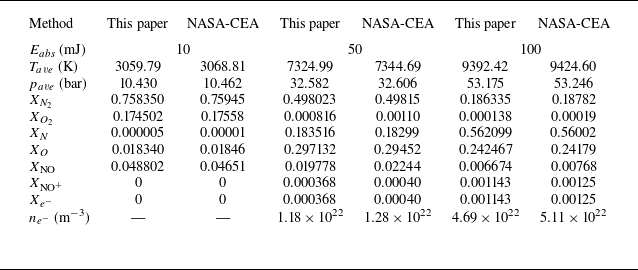

 a
 b


 100mJ
 a
 g
 h
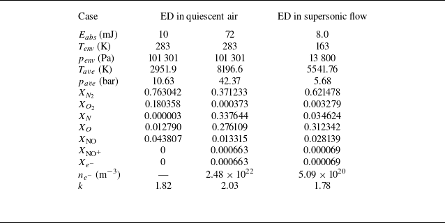

 72mJ
 a
 b
 c
 d


 t=0.5

 t=2.5

 t=5

 t=7.5


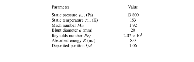

 ΔED
 Δy1
 700×450
 1000×660
 1300×850


 t=36.5

 t=44.8

 t=47.4

 t=54.2

 t=180

 t=250

 14

 26

 30

 54

 138

 214

 Ebase=72mJ

 t=90
 ρ/ρ∞
 T/T∞
 0.5Ebase
 Ebase
 1.5Ebase
 Ebase=72mJ
 Lj
 Dj
 Lj
 Dj

 0.5Ebase
 Ebase
 1.5Ebase
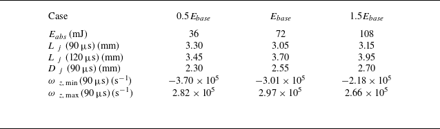

 βx,base=700m−1
 βr,base=1050m−1

 0.5βx,base
 1.2βx,base
 0.5βr,base
 1.2βr,base

 0.5βx,base
 0.8βx,base
 1.2βx,base
 βx,base=700m−1
 Lj
 Dj

 0.5βr,base
 0.8βr,base
 1.2βr,base
 βr,base=1050m−1
 Lj
 Dj

 Lj
 βx,base=700m−1
 βr,base=1050m−1
 Eabs=72mJ

 0.5βx,base
 0.8βx,base
 1.2βx,base

 βx,base=700m−1
 βr,base=1050m−1

 0.5βr,base
 0.8βr,base
 1.2βr,base

 βr
 RaL=0.060mm
 RbL=0.140mm
 RaR=0.070mm
 RbR=0.400mm


 +

 +

 +


