3.1. Linear regime

In the linear regime we recover the classical dynamics: at the time scale of order $10T_0$ after the start of the forcing, where $T_0=2{\rm \pi} /\omega _0$ is the forcing period, iterative focusing downscales the wave motion from the global scale $L$ to the scale associated with the width of the wave beams (Rieutord et al. Reference Rieutord, Georgeot and Valdettaro2000; Grisouard et al. Reference Grisouard, Staquet and Pairaud2008; Hazewinkel et al. Reference Hazewinkel, van Breevoort, Dalziel and Maas2008). Typical wave patterns observed in the quasi-linear regime at $t=17 T_0$ in horizontal and vertical planes are presented in the upper rows of figures 3 and 4 in terms of the quantities filtered at $\omega =\omega _0$ and $\omega =0$, respectively.

Figure 3.

Fields of radial $v_r$ and azimuthal $v_{\theta }$ velocity and vertical vorticity $\xi _{z}$ in the horizontal plane (at ${\simeq }20\ \mathrm {cm}$ depth) and of vertical velocity $v_z$ in the vertical plane. The presented quantities are filtered around $\omega =\omega _0$. Positive vorticity corresponds to cyclonic motion. The parallelogram with arrows in the vertical plane shows the theoretical attractor in which the energy propagates clockwise.

Figure 4.

Fields of radial $v_r$ and azimuthal $v_{\theta }$ velocity and vertical vorticity $\xi _{z}$ in the horizontal plane (at ${\simeq }20\ \mathrm {cm}$ depth) and of vertical velocity $v_z$ in the vertical plane. The presented quantities are filtered around $\omega =0$ with the low-pass filter having the upper cutoff frequency $\omega _c=\omega _0/3$. Positive vorticity corresponds to cyclonic motion.

Note that the width of the low-pass filter is set by the upper cutoff frequency, i.e. $\omega _c=\omega _0/3$. As discussed later, the essential low-frequency content of the experimental signal (see figure 8) lies well below the chosen cutoff frequency. The choice of the width of the low-pass filter is important for a unified description of numerical and experimental results (see §§ 4.4 and 4.5 for details). For the experimental results as such the choice of the cutoff frequency is less important (i.e. a lower value of $\omega _c$ could be prescribed). For the sake of brevity, the result of the low-pass filtering is below referred to as the ‘signal filtered at $\omega =0$’.

For clarity, we visualise the fields of radial $v_{r}$ and azimuthal $v_{\theta }$ velocity, vertical vorticity $\xi _{z}$ in the horizontal (equatorial) plane and the corresponding field of vertical velocity in the vertical (meridional) plane. It can be seen that the wave pattern observed at the forcing frequency (figure 3) in the horizontal plane is to a good approximation axisymmetric, while in the vertical trapezoidal cross-section we recover a classic pattern of the $(1,1)$ wave attractor (Maas et al. Reference Maas, Benielli, Sommeria and Lam1997; Maas Reference Maas2001) in agreement with the ray tracing, whose branch width is due to an equilibrium between wave focusing and viscous dissipation (Rieutord et al. Reference Rieutord, Georgeot and Valdettaro2000; Grisouard et al. Reference Grisouard, Staquet and Pairaud2008; Hazewinkel et al. Reference Hazewinkel, van Breevoort, Dalziel and Maas2008). The experimental signal filtered around $\omega =0$ remains weak at $t=17T_0$ (see figure 4).

3.2. Nonlinear regime

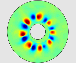
The development of the fully saturated nonlinear regime is illustrated in figures 3 and 4 by snapshots corresponding to $t=50T_0$ and $t=150T_0$. The full vortex pattern representing the slow 2-D manifold is formed at the time scale of $100T_0$. It can be clearly seen that the initial axisymmetry observed at $t=17T_0$ is lost while the slow manifold is gradually formed. The latter is represented by a regular polygonal system of eight cyclonic vortices. The vortices are nearly invariant in the vertical direction as attested by the right column of images in figure 4, representing the vertical velocity component. These vortex structures are reminiscent of the Taylor columns usually found in rotating systems but there is, however, a crucially important distinction: while the Taylor columns are normally formed as a consequence of a slow motion of a perturbation imposed on the rotating fluid, the coherent structures seen in figure 4 arise due to a nonlinear process which drains energy from the wave field toward the slow 2-D manifold. We note that the vertical velocity in the cyclonic vortices is directed downwards, corresponding to Ekman pumping, in agreement with existing experimental and numerical data (e.g. Hopfinger et al. Reference Hopfinger, Browand and Gagne1982; Godeferd & Lollini Reference Godeferd and Lollini1999). Interestingly, Lopez et al. (Reference Lopez, Hart, Marques, Kittelman and Shen2002) observed a similar breaking of a flow, axisymmetrically forced by a counter-rotating surface lid introducing azimuthal shear, into a discrete pattern of vortices distributed with an azimuthal periodicity. In their experiment, they relate the formation of such a manifold to the linear instability of the shear layer producing an azimuthal wave-like structure and, although much of the dynamics following the development of this instability is similar to the one we describe – e.g. the formation of a polygonal pattern of cyclonic vortices, intensified due to vortex stretching – the mechanism is different. In our set-up, the forcing introduces vertical motion in the fluid, and very little azimuthal motion is present at the beginning. As we will show in the numerical section, the instability observed in the nonlinear regime (figures 3 and 4) is then likely due to a triggered TRI that grows and becomes itself unstable. An internal boundary layer is formed around the attractor, which is prime candidate for the mixing of angular momentum, resulting in a sheared mean flow. It is worth mentioning that even in the fully saturated regime one can still identify the branches of the inertial wave attractor in the signal filtered around the forcing frequency $\omega =\omega _0$ (see figure 3). The relevance of such experimental regime (where a wave attractor in the meridional plane co-exists with a polygonal vortex system in the equatorial plane) to geo- and astrophysical systems admitting the existence of inertial wave attractors (Dintrans et al. Reference Dintrans, Rieutord and Valdettaro1999; Rieutord et al. Reference Rieutord, Georgeot and Valdettaro2001; Rieutord & Valdettaro Reference Rieutord and Valdettaro2010) represents an interesting direction for future research.

The visual evidence of the vortices is seen in figure 5 which presents the temporal evolution of the radial structure measured by sampling the azimuthal distribution of radial velocity at the radius $r= 8\ \mathrm {cm}$ corresponding to the position of centres of vortices seen in figure 4. Figure 5 shows that coherent structures start to appear after approximately $25T_0$, and that, further, the vortex pattern self-organises so that new structures gradually appear and join the ensemble. After approximately $100T_0$ all structures move at the same rate in cyclonic direction. This rate corresponds to half a turn of the vortex cluster around the inner cylinder which lasts approximately $(88 \pm 2) T_0$.

Figure 5.

Temporal evolution of the radial velocity as a function of azimuth, $\theta$, obtained by taking profiles of radial velocity at radius $r= 8\ \mathrm {cm}$ in the horizontal plane at ${\simeq }20\ \mathrm {cm}$ depth. To guide the eye, we added a solid line showing that the cluster rotates half a turn (${\rm \pi} \ \mathrm {rad}$) in $(88 \pm 2) T_0$.

The vertical vorticity field in the horizontal plane can be characterised statistically, by measuring the PDF of the micro-Rossby number $Ro^{\xi _{z}}=\xi _{z}/(2\varOmega )$. The typical PDFs of $Ro^{\xi _{z}}$ corresponding to different stages of development of the coherent vortex structures are shown in figure 6. We calculate the PDFs for the raw signal and for the signal filtered around the forcing $\omega =\omega _0$ and $\omega =0$ frequencies. The PDFs are calculated over the surface of the ring-shaped zone between the inner and outer cylinders, and over the time span of $\pm 2T_0$ around the time instances indicated in figure 6. It can be seen that at the beginning of the process, when the motion is represented essentially by the axisymmetric waves, the PDFs of $Ro^{\xi _z}$ have a sharp symmetrical form. As the nonlinear energy transfer towards coherent vortex structures develops, there is a progressive evolution of the vorticity PDFs toward the shape characterised by asymmetric ‘shoulders’, which indicates a well-pronounced cyclonic/anticyclonic asymmetry. This asymmetry is clearly seen in the PDFs calculated over the raw signal and the signal filtered around zero frequency $\omega =0$ (figure 6a,c), suggesting that a few strong cyclonic vortices seen in figure 4 are responsible for the asymmetry of the PDFs. The PDFs calculated for the signal filtered at the forcing frequency (figure 6b) remain approximately symmetrical at any time. A slight asymmetry visible in the curve corresponding to time around $t=30T_0$ and $40T_0$ can be tentatively attributed to the process of genesis of the regular polygonal vortex pattern: new cyclonic vortices are emerging in the plane of visualisation and are joining the ensemble. Nonetheless, since the asymmetry is weak one cannot exclude also a minor contribution from experimental noise.

Figure 6.

The PDFs of the vertical vorticity component at different times in the experiment. The curves (a–c) correspond to processing of the raw signal, and the signal filtered around $\omega =\omega _0$ and $\omega =0$.

4.1. Numerical procedure

The experimental section of this paper provides an important reference result: we explicitly show that, under sufficiently strong forcing, the motion in the system represents a nonlinear combination of a complex inertial wave field, with an identifiable wave attractor at the forcing frequency, and a slow quasi-2-D manifold represented by a PVC. In the numerical simulations described below, we faithfully reproduce the geometry of the set-up shown in figure 1, and we use the experimental value of the rate of background rotation $\varOmega =2.093\ \mathrm {rad}\ \mathrm {s}^{-1}$ and the forcing frequency $\omega _0=1.70\ \mathrm {rad}\ \mathrm {s}^{-1}$. We explore the effect of the forcing amplitude $a$ on the long-term nonlinear evolution of the inertial wave field in the set-up. Our purpose is to identify a sequence of observed regimes, ranging from the linear to the nonlinear regimes with a PVC described in the previous section.

The mathematical formulation of the problem consists in the Navier–Stokes equations and the continuity equation

(4.1)\begin{gather} \frac{\partial \boldsymbol{v}}{\partial t} + \left(\boldsymbol{v} \boldsymbol{\cdot} \boldsymbol{\nabla}\right) \boldsymbol{v} ={-}\boldsymbol{\nabla} {\tilde{p}} + \nu \Delta \boldsymbol{v} + 2{\boldsymbol{\varOmega}}\times \boldsymbol{v}, \end{gather}

(4.2)\begin{gather}\tilde{p} = \frac{p}{\rho} - \frac{1}{2}\left|{\boldsymbol{\varOmega}} \times \boldsymbol{r}\right|^2, \end{gather}

(4.3)\begin{gather}\boldsymbol{\nabla}\boldsymbol{\cdot} \boldsymbol{v} = 0, \end{gather}

with $\boldsymbol{v}$ the velocity field and $\tilde{p}$ the pressure field. The governing equations are written in the Cartesian system $(x,y,z)$, co-rotating with the set-up, where the $z$-axis points upwards and coincides with the axis of rotation. The origin of the coordinate system is taken at the centre of the upper lid. Note that the fixed lid has no inherent rotation in the rotating system $(x,y,z)$. In the fixed inertial non-rotating reference frame we define the anti-clockwise background rotation $\varOmega$ as positive. In the rotating reference frame the cyclonic vorticity is positive, and the sense of the prograde motion is positive – cyclonic is by definition in the direction of rotation; here we take a right-handed Cartesian coordinate system such that in cylindrical coordinates, $(r,\theta , z)$, the azimuthal coordinate $\theta$ increases in cyclonic direction. With this convention the cyclonic vortices appear in red colour both in numerical and experimental vertical vorticity patterns. If the motion in a vertical radial plane is considered (e.g. plane $y=0$) we use the notations $(r,z)$. Throughout the paper we visualise the fluid motion in the horizontal plane located at mid-depth of the fluid volume.

To complete the mathematical statement of the problem we prescribe the boundary conditions as follows: the no-slip condition is imposed at all rigid boundaries except at the fixed flat horizontal upper lid where a specific harmonic forcing is applied to simulate the experimental one. We thus require that both horizontal components of the fluid velocity vector at the upper lid are equal to zero as in standard no-slip condition, while the vertical component is prescribed as explained below. Figure 2 shows the discrete experimental profile of the amplitude of motion of the rings in the generator. This discrete stepwise form approximates the smooth profile $z(r)$ shown in figure 2 by the dashed blue line. The forcing imposed in the numerical experiments at the upper lid is axisymmetric, with the vertical component of the fluid velocity given by $v_{z}(r,t)=a\tilde {z}(r)\omega _0\exp (\omega _0 t)$ where $a$ is the forcing amplitude and $\tilde {z}(r)$ is a non-dimensional profile (of unit amplitude at $r=R_0$) such that $z(r) = a \tilde {z}(r)$ corresponds to the dashed blue curve of figure 2. Since we consider a small-amplitude input perturbation (more precisely, $a/(R_1-R_0) \leqslant 0.0167$), such an approach seems to be justified. In the case of internal wave attractors with similar implementation of the input forcing, we observed a good qualitative agreement between numerical and experimental results (Brouzet et al. Reference Brouzet, Sibgatullin, Scolan, Ermanyuk and Dauxois2016b). However, an extension to rotating fluids stratified in angular momentum, and not in density, and driven by Coriolis force (which does no work), and not by gravity (which does), is not fully evident. Both this issue and the difficulty of precise evaluation of the efficiency of the experimental wave generator leaves a considerable margin of uncertainty regarding the possible correspondence between the experimental amplitude and its numerical counterpart.

The numerical simulations have been performed for the following set of $7$ forcing amplitudes: $a=0.2$, $0.5$, $1.0$, $1.8$, $2.0$, $2.4$, $2.5$ mm, the latter value corresponding to the experimental case. This corresponds to Rossby numbers $Ro^L$ ranging from $5 \times 10^{-4}$ to $7 \times 10^{-3}$. Below, we use a reduced representative set of amplitudes to describe the key regimes observed. The typical duration of the numerical experiments was approximately $200 T_{0}$, and in some cases up to $350 T_{0}$ (e.g. at $a=2.4$ mm).

As evident from the experimental part of the paper, we need to model a strongly nonlinear dynamical problem, where both viscosity and nonlinearity play a role. The numerical simulation of transient and turbulent regimes is a challenge as we have to follow the development of small-scale structures during long time intervals. In this context, spectral or Galerkin decomposition is known to be a robust approach to tackle the nonlinear effects without parasitic effects due to numerical viscosity. Classically, such a decomposition is possible only for simple geometry and boundary conditions. In the present work the direct numerical simulations are performed with the help of the spectral element method, using the open source code Nek5000 (see Fischer & Ronquist Reference Fischer and Ronquist1994; Fischer Reference Fischer1997; Deville, Fischer & Mund Reference Deville, Fischer and Mund2002). This method combines the advantages of high-order decomposition with geometric flexibility, and permits to run long-term simulations of strongly nonlinear dynamics. In the present study, we have used meshes with up to $100$ thousand elements, with eighth-order polynomial decomposition within each element (up to $50$ millions degrees of freedom).

4.2. Energy spectra: a preliminary classification of the observed regimes

The snapshots of the simulated inertial wave fields in horizontal and vertical planes are shown in figure 7 for a set of forcing amplitudes $a=0.2$, $1.0$, $2.0$, and $2.4$ mm at $t=100T_0$ (all images correspond to the same phase of the forcing). As the amplitude increases, one observes the increasing complexity of the inertial wave fields, in broad agreement with the known literature on the onset of TRI (Bordes et al. Reference Bordes, Moisy, Dauxois and Cortet2012; Bourget et al. Reference Bourget, Dauxois, Joubaud and Odier2013) and wave turbulence in internal and inertial wave attractors (Brouzet et al. Reference Brouzet, Ermanyuk, Joubaud, Sibgatullin and Dauxois2016a,Reference Brouzet, Sibgatullin, Scolan, Ermanyuk and Dauxoisb). In particular, one can see (i) visible broadening of the attractor branches at higher forcing (Brouzet et al. Reference Brouzet, Sibgatullin, Ermanyuk, Joubaud and Dauxois2017b), (ii) the signature of discrete azimuthal symmetry in the vertical vorticity pattern in horizontal plane at $a=1.0$ mm in agreement with preliminary simulations described in Sibgatullin et al. (Reference Sibgatullin, Ermanyuk, Maas, Xu and Dauxois2017) and (iii) the emerging signature of discrete patches of vertical vorticity in the horizontal plane at $a=2.4$ mm which are reminiscent of the experimental observations described in § 3. Below, we apply a set of post-processing tools to analyse the numerical data in some detail.

Figure 7.

Snapshots of the vertical vorticity field, obtained by numerical simulations, in horizontal plane at mid-depth $z=-20$ cm (a–d) and corresponding vertical velocity fields in vertical plane $y=0$ (e–h) taken at $t=100T_0$ at different values of the forcing amplitude $a$. Note that both in experiments and in numerical computations we denote cyclonic vorticity and prograde azimuthal velocity as positive. Thus the experimental and numerical patterns have the same colour coding and can be directly compared regardless of the direction of the background rotation.

The nonlinear regimes observed in the numerical simulations of an axisymmetrically forced inertial wave attractor can be roughly classified by considering the development of the signal spectra with time for a set of forcing amplitudes. The typical time–frequency diagrams obtained at different values of $a$ are shown in figure 8. These diagrams are calculated similarly to Bourget et al. (Reference Bourget, Dauxois, Joubaud and Odier2013), as follows

(4.4)\begin{equation} S_r(\omega,t)=\left\langle \left| \int_{-\infty}^{+\infty} v_r(r,\theta,\tau)\textrm{e}^{\textrm{i}\omega \tau}h(t-\tau)\, \mbox{d}\tau \right|^2\right\rangle_{r\theta}, \end{equation}

where $h$ is a Hamming window and $v_r$ is the radial component of the velocity field, and subscript $r\theta$ denotes a ring-shaped domain around the inner cylinder ($\theta \in [0, 2{\rm \pi} ]$, $r \in [5, 10]$ cm). The calculations are performed with the Matlab toolbox described in Flandrin (Reference Flandrin1999). The time–frequency diagrams were also calculated for other variables (e.g. azimuthal velocity, vertical vorticity), demonstrating similar qualitative behaviour.

Figure 8.

Time–frequency diagram of the logarithm (colour) of the normalised spectrum of the radial velocity, $S_r(\omega ,t) / \langle S_0 \rangle$, where $\langle S_0 \rangle$ is the time averaged spectrum at $\omega /\omega _0=1$, calculated with the help of (4.1) for a ring-shaped region around the inner cylinder ($r \in [5, 10]$ cm). The last image in the lower row corresponds to the time–frequency diagram calculated for the experimental data obtained at $a=2.5$ mm. The white dashed line indicates the cutoff frequency $f$.

The signatures of inertial wave turbulence can be detected by analysing the energy spectra (Yarom & Sharon Reference Yarom and Sharon2014). Note that the original approach implying 4-F Fourier analysis (three dimensions for space and one for time) has been proposed by Yarom & Sharon (Reference Yarom and Sharon2014) for a rotating system where the energy is injected via decorrelated random forcing thereby creating well-developed fully 3-D wave turbulence possessing no information on initial orientation of the input wave vector. In the present paper the energy is injected via axisymmetric deterministic forcing (with prescribed amplitude, length and frequency) producing a variety of dynamic regimes ranging from regular to turbulent (see figure 7). In order to adapt the method of post-processing to the observed wave patterns, we perform the analysis described in Yarom & Sharon (Reference Yarom and Sharon2014) in a vertical radial plane similar to Brouzet et al. (Reference Brouzet, Ermanyuk, Joubaud, Sibgatullin and Dauxois2016a), and, in addition, calculate the spatial energy spectrum in a horizontal plane. The latter is done to clarify the role of the integer-number azimuthal modes at different values of the forcing amplitude. Note that owing to different design of the experimental set-up such modes were not present in the case studied by Yarom & Sharon (Reference Yarom and Sharon2014). Before computing the energy spectra, the numerical results are re-sampled to yield the spatial resolution of $0.2\ \textrm {cm} \times 0.2\ \textrm {cm}$ and the temporal resolution of $0.2$ s. This is done to reduce the amount of data and to match the typical experimental resolution. The wave-energy spectra in the vertical radial plane are computed using the 3-D Fourier transforms of the horizontal and vertical velocity fields, $\hat {v}_{r}(k_r,k_z,\omega )$ and $\hat {v}_{z}(k_r,k_z,\omega )$. The corresponding energy spectrum is defined as

(4.5)\begin{equation} E_\parallel(k_r,k_z,\omega)=\frac{|\hat{v}_{r}(k_r,k_z,\omega)|^2+|\hat{v}_{z}(k_r,k_z,\omega)|^2}{2A_\parallel T}, \end{equation}

where $A_\parallel =40\times 15\ \textrm {cm}^2$ is the area considered in the vertical plane and $T=50T_0$ is the duration of the time-history sample. The calculations for all the cases shown below in figure 9 are performed for the numerical data obtained for $t \in [100T_0, 150T_0]$. The spatial resolution of re-sampled data and the size of the fluid domain provide respectively the upper and lower bounds in wavenumbers, of order $k_{max}=8\ \mathrm {rad}\ \mathrm {cm}^{-1}$ and $k_{min}=0.2 \ \mathrm {rad}\ \mathrm {cm}^{-1}$. Interpolation is performed to express the energy spectrum $E_\parallel (k_r,k_z,\omega )$ as a function of $E_\parallel (k,\alpha ,\omega )$, with $k$, the norm of the wave vector. Then, we perform integration over the entire range of resolved wave vectors $[k_{min}, k_{max}]$ as follows:

(4.6)\begin{equation} E_\parallel(\alpha,\omega)=\int_{k_{min}}^{k_{max}}E_\parallel(k,\alpha,\omega)k \,{\mathrm{d}}k. \end{equation}

The calculated energy density $E_\parallel (\alpha ,\omega )$ is normalised by the frequency energy density $E_\parallel (\omega )$, obtained by integrating $E_\parallel (\alpha ,\omega )$ over all directions. It should be stressed that it is only for a purely axisymmetric wave perturbation that $E_\parallel (\alpha ,\omega )$, defined by (4.6), is a function of the true angle $\alpha$ between the vector of the phase speed and the horizontal plane. In the axisymmetric case, the vector $(k_{r},k_{z},k_{\theta })$ has $k_{\theta }=0$, where the direction of the component $k_{\theta }$ is defined by a vector orthonormal to the $(r,z)$ plane. In the general case, the vector $(k_{r},k_{z},k_{\theta })$ is inclined at an angle $\alpha =\arctan [k_{z}/(k_{r}^2+k_{\theta }^2)^{1/2}]$ to the vertical axis. A projection of this vector onto the vertical $(r,z)$ plane is seen at the apparent angle $\alpha _{*}=\arctan [k_{z}/k_{r}]$. Restricting, for brevity, our attention to small values of $\alpha$ and $\alpha _{*}$, the difference between the two angles can be quantitatively characterised as $[1+(k_{\theta }^2/k_{r}^2)]^{1/2} - 1$. For example, the relative difference $|(\alpha _{*}-\alpha )/\alpha |<0.1$ translates to $|k_{\theta }/k_{r}|<0.46$, thereby admitting the vectors whose azimuthal direction differs from the $(r,z)$ plane by less than ${\pm }25^{\circ }$.

Figure 9.

The upper four images present the normalised energy spectra $(E_\parallel (\alpha ,\omega )/E_\parallel (\omega ))$ at different values of the forcing amplitude. Colours indicate the levels of normalised energy spectra. The white dashed lines correspond to the dispersion relation $\pm \cos \alpha =\omega /f$. Note that the energy peaks are not always localised at the dispersion curve, owing partially to the departure of the wave vectors from $(r,z)$ plane and to the contribution of slaved (evanescent) waves (see discussion in the text). The lower four images show the energy spectra in the horizontal plane $E_\perp (k_{r},n_{\theta })$ on a logarithmic scale at different values of the forcing amplitude. By combining information from the spectra calculated in the vertical and horizontal planes one can see the evolution of wave regimes from nearly linear at $a=0.2$ mm to wave turbulence evolving from a ‘discrete’ form at $a=1.0$ to a more ‘continuous’ form at $2.0$ and $a=2.4$ mm. The latter is particularly well seen in terms of $E_\perp (k_{r},n_{\theta })$. In all cases the axisymmetric component of the wave field (corresponding to $n_{\theta }=0$) is most significant.

An additional analysis is performed in the horizontal plane located at the mid-depth of the set-up. The wave-energy spectrum in the horizontal plane is computed using the 3-D Fourier transform of the horizontal components of the velocity field, $\hat {v}_{r}(k_r,n_{\theta },\omega )$ and $\hat {v}_{\theta }(k_r,n_{\theta },\omega )$. Here, $n_{\theta }=2{\rm \pi} /\Delta \theta$ is the non-dimensional azimuthal wavenumber, where $\Delta \theta$ is the azimuthal wavelength (in radians). Note that using $n_{\theta }$ is more convenient than using $k_{\theta }$ (measured in $\mathrm {rad}\ \mathrm {m}^{-1}$) in view of the discrete azimuthal symmetry of the wave patterns in the horizontal plane clearly seen in figure 7 at $a=1.0$ mm. The corresponding energy spectrum is defined as

(4.7)\begin{equation} E_\perp(k_r,n_{\theta},\omega)=\frac{|\hat{v}_{r}(k_r,n_{\theta},\omega)|^2+|\hat{v}_{\theta}(k_r,n_{\theta},\omega)|^2}{2A_{r,\theta}T}, \end{equation}

where $A_{r,\theta }$ is the area considered ($r \in [R_0,R_1]$, $\theta \in [0,2{\rm \pi} ]$) and $T=50T_0$ is the duration of the time-history sample. The spectrum is integrated over the frequency range $\omega \in [-f,f]$ in which inertial waves can propagate, as follows:

(4.8)\begin{equation} E_\perp(k_r,n_{\theta})=\int_{{-}f}^{f}E_\perp(k_r,n_{\theta},\omega)\,{\mathrm{d}}\omega. \end{equation}

Using (4.4), (4.6) and (4.8), we obtain figures 8 and 9, which show the time–frequency diagram of the logarithm of the normalised spectrum of the radial velocity, and the energy spectra $E_\parallel$ and $E_\perp$ at different forcing amplitudes, respectively. From these figures we can infer information on the qualitative evolution of the wave regime with amplitude. It can be seen in figure 8 that for the lowest amplitude considered ($a=0.2$ mm), the frequency spectrum is monochromatic, with a weak but detectable component at twice the forcing frequency. This is confirmed by the energy spectrum for this amplitude represented in figure 9: the energy is localised on the linear dispersion relation at discrete ‘spots’ corresponding to $\omega _0/f=0.39$ and $2\omega _0/f=0.78$. The perturbation is nearly axisymmetric, a weak contribution of low azimuthal modes can be detected in terms of $E_\perp (k_{r},n_{\theta })$.

At higher forcing amplitude ($a=1.0$ mm), one can observe (see figure 8) a classic signature of TRI. One can see signal components at the frequencies of two most energetic secondary waves which satisfy the condition $\omega _0=\omega _1+\omega _2$, with $\omega _1/\omega _0=0.32$ and $\omega _2/\omega _0=0.68$ (here, the subscripts $0$, $1$ and $2$ denote the parameters of the primary wave, and two secondary waves). Also there is a significant energy content at frequencies $\omega _1+\omega _0$, $\omega _2+\omega _0$, and the multiples of the forcing frequency $2\omega _0$ and $3\omega _0$. Thus, both TRI and the two-wave interactions (Beckebanze et al. Reference Beckebanze, Grayson, Maas and Dalziel2021; Boury, Peacock & Odier Reference Boury, Peacock and Odier2021) are present in the system and play a role. The corresponding energy spectrum shown in figure 9 demonstrates that the linear dispersion relation attracts the energy maxima. However, some energy content falls apart from the dispersion relation, producing a pattern of weak horizontal stripes as consequence of the difference between angles $\alpha$ and $\alpha _{*}$ arising from quasi-2-D analysis (4.6). In terms of $E_{\perp }(k_{r},n_{\theta })$ we observe a contribution of low azimuthal modes, where significant peaks can be distinguished at $n_{\theta }=\pm 12$. As it will be discussed in § 4.3, this is related with spiral waves propagating in retrograde and prograde sense which are likely a consequence of triadic resonance. The data analysis presented in figures 8 and 9 for $a=1$ mm supports the idea that this regime corresponds to the onset of weak (discrete) inertial wave turbulence.

As the forcing amplitude increases further ($a=2.0$, $2.4$, and $2.5$ mm), one can observe a significant increase of the energy content in the continuous part of the frequency spectrum, accompanied by an enrichment of the discrete part (figure 8). The peaks corresponding to TRI-generated secondary waves $\omega _1$ and $\omega _2$ (detected at $a=1.0$ mm) remain persistent at higher forcing amplitudes. In general, the overall trends seen in figure 8 at higher forcing amplitudes correspond well to the effects described in the literature on internal wave attractors in stratified fluids in the nonlinear regime (Brouzet et al. Reference Brouzet, Ermanyuk, Joubaud, Sibgatullin and Dauxois2016a, Reference Brouzet, Ermanyuk, Joubaud, Pillet and Dauxois2017a). There is, however, an important distinction: in the case of rotating fluid we observe a highly complicated frequency content of the signal at the low-frequency end of the spectrum which does not have a straightforward interpretation in terms of TRI. In the context of this paper this issue is of central interest (see § 4.5 for discussion). Note that some discrete frequency components seen in the numerical calculations performed at $a=2.4$ and 2.5 mm appear also in the experimental spectrum. In the numerical simulations, the transients seem to have a significantly longer duration as compared with the experiment. This issue is discussed in § 4.5.

The energy spectra for higher forcing amplitudes shown in figure 9 seem to be consistent with the concept of inertial wave turbulence. As $a$ increases, the character of wave turbulence gradually evolves from a ‘discrete’ form at $a=1.0$ to a more ‘continuous’ form at $a=2.0$ and $2.4$ mm. The latter is particularly well seen in terms of $E_{\perp }(k_{r},n_{\theta })$. The presence of a significant continuous component in $E_{\perp }(k_{r},n_{\theta })$ is a direct consequence of the loss of the discrete azimuthal symmetry observed in figure 7 at $a=2.0$ and $2.4$ mm.

As the energy spectra $E_\parallel (\alpha ,\omega )$ are calculated in the vertical plane we can see that the structure of the low-frequency zones (where the dispersion relation crosses the line ${\omega /f=0}$) evolves considerably as $a$ increases. In the quasi-linear case ($a=0.2$ mm) there is no detectable energy component at $\omega /f\simeq 0$. As $a$ increases, a complex discrete structure emerges in the vicinity of $\omega /f\simeq 0$. At higher $a$ this structure evolves toward a smoothed energy distribution, which can be interpreted as a trend toward merging of energy peaks corresponding to discrete frequencies.

It has been already noted that some energy content falls apart from the dispersion relation due to the difference between $\alpha$ and $\alpha _{*}$ as a consequence of the 2-D analysis in (4.6). Let us note that there is an additional mechanism for the concentration of such peaks, namely along the vertical lines at fixed $\alpha$ corresponding to the forcing frequency $\omega _0$. This means that forced higher harmonics are generated which propagate at an angle belonging to that of the fundamental frequency, as opposed to free higher harmonics that follow the dispersion curves. These ‘slaved’ higher harmonics have been encountered in internal wave attractors before (Lam & Maas Reference Lam and Maas2008). An interested reader is relegated to Davis (Reference Davis2019), in which a similar phenomenon is observed and discussed in more detail.

4.3. Triadic resonant instability in a rotating annulus

Relevant to our study, let us consider in more detail the TRI in the rotating annulus. TRI has been observed in various configurations of rotating flows involving precession, and often led to symmetry breaking and to the formation of vortical structures distributed periodically (Albrecht et al. Reference Albrecht, Blackburn, Lopez, Manasseh and Meunier2015; Marques & Lopez Reference Marques and Lopez2015; Albrecht et al. Reference Albrecht, Blackburn, Lopez, Manasseh and Meunier2018; Lopez & Marques Reference Lopez and Marques2018; Wu, Welfert & Lopez Reference Wu, Welfert and Lopez2020a). For example, in the case of a rotating cylinder (e.g. Marques & Lopez Reference Marques and Lopez2015), this instability gives rise to structures aligned with the rotation axis and distributed along $\theta$.

The data presented in figure 8 for $a=1.0$ mm show well-localised discrete frequency components. Using the technique of Hilbert transform filtering introduced in Mercier, Garnier & Dauxois (Reference Mercier, Garnier and Dauxois2008), one can separate the key components of the wave patterns observed in vertical and horizontal planes as shown in figures 10 and 11. The filtered wave field components seen in the vertical plane remind of the patterns already described in literature for internal wave attractors (see e.g. Scolan et al. Reference Scolan, Ermanyuk and Dauxois2013; Brouzet et al. Reference Brouzet, Ermanyuk, Joubaud, Pillet and Dauxois2017a). The length of the wave vector components can be evaluated with reasonable accuracy as location of the maximum of corresponding PDFs calculated over the domain of interest. The corresponding vector triad in vertical plane is shown in figure 12(a) together with the curves defining the admissible wave triads. It can be seen that the observed triad is consistent with the theoretical curve, with reasonable experimental accuracy.

Figure 10.

The components of the inertial wave field (displayed in terms of the vertical velocity component) filtered at frequencies $\omega _0$, $\omega _1$ and $\omega _2$ (a–c), with the corresponding phase patterns (d–f). Only one branch of the wave attractor is shown. The corresponding vector triad is shown in figure 12(a).

Figure 11.

The components of the vertical vorticity field $\xi _z$ filtered at frequencies $\omega _0$, $\omega _1$ and $\omega _2$ (a–c), with corresponding filtered wave fields as function of radial coordinate $r$ and azimuthal coordinate $\theta$, with amplitude shown in (d–f) and phase shown in (g–i). Note that the primary wave is axisymmetric and propagates radially, while the secondary waves corresponding to frequencies $\omega _1$ and $\omega _2$ propagate azimuthally in the prograde (cyclonic) and retrograde (anti-cyclonic) directions, respectively, and the azimuthal components of the wave vectors have the same length. The corresponding vector triad is shown in figure 12(b).

Figure 12.

Verification of the triadic resonance: (a) curve of admissible wave vector triads in the vertical plane $(k_r, k_z)$ with superimposed measured wave vectors; (b) wave vector triad in the horizontal plane $(k_r, n_\theta )$. The wave vector triads shown in the left and right panels represent their projections on the vertical and horizontal planes respectively, and correspond to the patterns depicted in figures 10 and 11. The solid, dashed, and dash-dotted lines in panel (a) represent the locus of the tips of the resonant wave vectors according to the dispersion relation.

The pattern of triadic resonance in a ring-shaped domain seen in the horizontal plane possesses a discrete symmetry as shown in figure 11. This is in agreement with earlier observations described in Sibgatullin et al. (Reference Sibgatullin, Ermanyuk, Maas, Xu and Dauxois2017), and with raw snapshots shown in figure 7 for $a=1.0$ mm in the present paper. Thus, the azimuthal pattern in the horizontal plane is reminiscent of ‘modal’ triadic resonance in a rectangular box described in McEwan (Reference McEwan1971). However, the modal pattern of internal waves in the vertical plane (McEwan Reference McEwan1971) is clearly compatible with the dispersion relation, while we are not aware of any theoretical work predicting the number of the expected azimuthal mode of the secondary waves in a ring-shaped domain. Note, however, that Lin, Noir & Jackson (Reference Lin, Noir and Jackson2014) and Lagrange, Meunier & Eloy (Reference Lagrange, Meunier and Eloy2016) have looked at this in slightly different geometries (such as a different orientation of the cylinder axis). Assuming the triadic resonance as the underlying key mechanism and a discrete symmetry of the azimuthal wave pattern, we can expect that the purely axisymmetric wave (i.e. zero azimuthal mode) at the forcing frequency $\omega _0$ should give rise to two secondary waves propagating in the opposite azimuthal directions (cyclonic and anti-cyclonic) and corresponding to the same azimuthal mode. This is confirmed by the data presented in figure 11 and by the construction of the projection of the wave vector triad on the horizontal plane shown in figure 12(b). Both secondary waves seen in the horizontal plane correspond to 12-th azimuthal mode. The secondary waves corresponding to $\omega _1$ and $\omega _2$ propagate in cyclonic and anti-cyclonic directions, respectively.

Summing up, we can characterise each wave component by three numbers $(k_{r},k_{z},n_{\theta })$, where $k_{r}, k_{z}$ are conventional wave vector components measured in $r,z$-plane (in $\mathrm {rad}\ \textrm {cm}^{-1}$), while $n_{\theta }=2{\rm \pi} /\Delta \theta$ is non-dimensional integer azimuthal mode number, where $\Delta \theta$ is the azimuthal wave length (in radians). For the vector triads depicted in figure 12, we have $(1.38,0.94,0)$, $(-1.88,-0.43,-12)$ and $(3.02,1.26,12)$ for the primary and two secondary waves, respectively. With reasonable accuracy we have $k_{r}^0 \approx k_{r}^1+k_{r}^2$, $k_{z}^0 \approx k_{z}^1+k_{z}^2$ and $n_{\theta }^0=0=n_{\theta }^1+n_{\theta }^2$. It should be stressed that the wave vector components can be strictly defined only for spatially monochromatic fields (or approximately monochromatic as in Bourget et al. Reference Bourget, Dauxois, Joubaud and Odier2013) while for narrow wave beams the objective measurement of wave vector components raises some problems as discussed in Fan & Akylas (Reference Fan and Akylas2020). However, experimentally it is often possible to construct the PDFs for the wave vector components measured in a zone of interest and estimate the length of the wave vectors from the positions of PDF's maxima. This approach is taken in the present paper. In light of the results presented in figure 12, we note that the resonance conditions for TRI are satisfied here. Moreover, it is interesting to point out that the primary wave is three-dimensional but axisymmetric, and therefore mostly lives in a vertical plane, contrary to the two secondary waves, which are non-axisymmetric and fully three-dimensional. At this stage, however, the discussion of this $3$-D TRI is purely exploratory. The reader interested in a more thorough development is referred to Boury (Reference Boury2020) (§ 7.5.2).

4.4. Transition to a PVC

Let us now consider how the regime in which a PVC emerges in the numerical simulations when we systematically increase the forcing amplitude. By considering the results obtained at $a=1.0$ mm we have already made an important observation that the low-frequency behaviour of the system is represented by cyclonic propagation of a secondary wave generated by triadic resonance. In other words, we can say that, after the onset of TRI, this low-frequency component of the wave field represents a ‘germ’ of the slow manifold. Therefore, to compare the flow patterns representing the slow manifold in the horizontal plane it is reasonable to use the low-pass filtering with the cutoff frequency set around $\omega _c=\omega _0/3$. The width of this filter corresponds to the width of the filter used in the experimental part of the paper to separate the low-frequency signal. Moreover, the time–frequency diagrams shown in figure 8 allow us to conclude that this width of the low-pass filter captures the essential features of the low-frequency behaviour of the system. By applying this filter we can identify the variation of the structure of the vertical vorticity field at different forcing amplitudes, as shown in figure 13. The snapshot of the pattern is complemented by a video in supplementary material available at https://doi.org/10.1017/jfm.2021.703. The snapshots and the video are taken in vicinity of the time instant $t=100T_0$. It can be clearly seen that the cyclonic wave motion at $a=1.0$ mm is replaced by a highly complicated pattern which exhibits cyclonic/anti-cyclonic rotation close to the inner/outer cylinder, respectively. We illustrate such a regime by the data obtained at $a=2.0$ mm. This regime is observed in a certain range of the forcing amplitudes (around $a\in [1.8\ \mathrm {mm};2.0\ \mathrm {mm}]$). Thus, the transition from the regime with wave field possessing discrete azimuthal symmetry ($a=1.0$ mm) to the regime with PVC ($a=2.4$ mm) is highly non-trivial. The intermediate regime observed at $a=2.0$ mm deserves a special study which falls outside of the scope of the present paper.

Figure 13.

The low-frequency pattern of the vertical vorticity field filtered by low-pass filter with the cutoff frequency $\omega _c=\omega _0/3$ at different values of the forcing amplitude in the DNS and for the experimental case. The images correspond to the time $t=100 T_0$. In the supplementary material we provide a short video of this pattern demonstrating prograde motion of the wave pattern at $a=1.0$ mm, prograde/retrograde motion close to inner/outer cylinder respectively at $a=2.0$ mm and prograde motion of the vortex cluster at $a=2.4$ mm (in numerical simulations) and at $a=2.5$ mm (in experiments). Note that for experimental data we take a mirror image, so that the background rotation and prograde motion are anti-clockwise. The numerically calculated wave/vortex patterns are rotating around the central cylinder while interacting with the mean azimuthal currents shown in the right panel of figure 17.

As the forcing amplitude increases further, one can clearly identify the patches of cyclonic vorticity arranged in polygonal fashion, with a slow drift of the vortex cluster in prograde direction. This regime is shown in figure 13 for $a=2.4$ mm. A very similar regime is observed at $a=2.5$ mm, which suggests that the regime is sufficiently robust and can be reproduced in a certain range of the forcing amplitudes. The numerically obtained vortex pattern with $7$ vortices arranged at the vertices of a regular polygon can be compared with the experimental vortex pattern with $8$ vortices. We see that qualitatively the patterns are similar, and, since the colour scale for both patterns is the same, at quantitative level there is a reasonable agreement between the magnitudes of the vertical vorticity. However, the mechanism of the formation of the vortex patches and the long-term evolution of the pattern in the numerical calculations remain to be identified. To do this we performed a long series of calculations specifically for this regime at $a=2.4$ mm. The results of these simulations are described below.

Our results point towards the existence of a transition between two different regimes, one dominated by weakly nonlinear effects and the onset of TRI at low forcing amplitude, and another one characterised by the existence of a PVC at higher forcing amplitudes. As suggested by the numerical data presented in figures 8, 9 and 13, this transition is likely to occur between $a=1.0$ and $a=2.0\ \mathrm {mm}$. The experimental results fall into the second case with the fully developed PVC manifold. This transition is also evidenced by the change in characteristic Reynolds number, computed at the wave scale, as shown in table 1, since its order of magnitude changes from $10$ to $100$ between these two regimes, thus indicating stronger and more efficient energetic transfers between scales. However, no obvious scaling of $Re$ with $a$ could be found, and a detailed study of this transition falls beyond the scope of this study.

Table 1.

Estimation of the Reynolds number $Re$, computed at the wave scale, at $t=200T_0$ in the numerics and in the experiment.

4.5. Long-term fate of the PVC in numerical simulations

As previously mentioned, at relatively high forcing amplitudes the system evolves in a state where the formation of vertical vortices organised periodically around the inner cylinder becomes the characteristic feature. We present in figure 14 a 3-D numerical visualisation of this transition in the case of the forcing amplitude $a=2.4\ \mathrm {mm}$, using $\lambda _2$ isosurfaces computed based on the method proposed by Jeong & Hussain (Reference Jeong and Hussain1995). The snapshots are taken at three different times and show the laminar regime (panel (a), at $t=13.5 T_0$), the transitional small-scale turbulent state (panel (b), at $t= 27.1 T_0$) and the developed regime (panel (c), at $t= 389.6 T_0$). Shortly after the beginning of the simulation, the flow becomes weakly turbulent and small-scale features can be detected close to the inner cylinder, before being reorganised into the well-defined vertical vortices consistently observed both in the DNS and in the experiments.

Figure 14.

Visualisation of the vorticity in the numerical simulation at forcing amplitude $a=2.4\ \mathrm {mm}$ using $\lambda _2$ isosurfaces, following the method detailed in Jeong & Hussain (Reference Jeong and Hussain1995). Snapshots are taken, from left to right, at $t=13.5 T_0$, $t= 27.1 T_0$ and $t= 389.6 T_0$.

The long-term time–frequency diagram corresponding to this forcing amplitude ($a=2.4$ mm) is presented in figure 15. The diagram is calculated over $350$ forcing periods. Window 6 shows schematically the domain where the low-pass filter with the cutoff frequency $\omega _c=\omega _0/3$ has been applied to obtain the vortex pattern depicted in figure 13 for $a=2.4$ mm. This pattern remains virtually the same over a long time span. In particular, the $7$-vortex cluster can be observed when window 6 is shifted in time to cover the narrow peaks 3 and 4. These peaks 3 and 4 are well localised, making possible a narrow-band filtering of the corresponding wave components of the vertical vorticity field. The result of such filtering is represented in figure 15 by the patterns corresponding to $\omega _3=0.36\ \mathrm {rad}\ \mathrm {s}^{-1}$ ($\omega _{3}/\omega _0=0.21$) and $\omega _4=0.16\ \mathrm {rad}\ \mathrm {s}^{-1}$ ($\omega _{4}/\omega _0=0.09$). The former represents a wave of seventh azimuthal mode propagating in the cyclonic (prograde) direction in the close vicinity of the inner cylinder, the positive and negative patches of vorticity in this wave have the same magnitude. The latter represents a wave of the fifth azimuthal mode propagating in the anti-cyclonic (retrograde) direction. Note that the wave corresponding to $\omega _{4}/\omega _0=0.09$ is significantly weaker in magnitude than the wave corresponding to $\omega _{3}/\omega _0=0.21$. Apart from this well-defined discrete components there is also a contribution from the continuous part of the spectrum. Thus, the $7$-vortex pattern seen in figure 13 can be interpreted as azimuthal wave of seventh mode propagating in prograde sense over weak background vorticity pattern. In this background pattern we can identify fifth azimuthal retrograde wave mode while other discrete wave contributions are difficult to identify. The observable result of such superposition is the polygonal $7$-vortex pattern.

Figure 15.

The time–frequency diagram corresponding to the case $a=2.4$ mm (a). (b–d) Show the snapshots of the vertical vorticity fields filtered in narrow frequency windows $3$ and $4$ around $t=170T_0$, and via low-pass filter schematically shown as $5$ around $t=310T_0$. Patterns $3$ and $4$ propagate in prograde and retrograde directions, respectively. Note that the discrete low-frequency components seen in the time–frequency diagram exhibit a trend toward merging at $t>225T_0$, and filter $5$ is applied to the result of the merging process. The result of filtering with $6$ (low pass-filter, earlier times) is shown in figure 13(c).

It should be noted that at long time scale the observable vortex pattern evolves. It can be seen in figure 15 that after approximately $225T_0$ the discrete frequency components at the low-frequency end of the spectrum exhibit a strong trend towards merging. Towards the time around $275T_0$ it becomes difficult to distinguish individual low-frequency wave components. The low-pass filtering applied to the domain schematically shown by rectangle 5 returns the vorticity pattern which develops as result of merging of the low-frequency discrete wave components. The resulting slow manifold is represented by a PVC with $8$ cyclonic vortices drifting in cyclonic direction. This pattern is very similar, in terms of strength and spatial arrangement of vortices, to the experimental pattern shown in figure 13. The evolution of the azimuthal drift of the vortex cluster with time is illustrated in figure 16 representing the numerical counterpart of figure 5. It can be seen that numerical simulations yield $6$ to $3$ times faster drift than the experimentally measured one. Note that the time–frequency diagram itself shows some discrepancies between the experimental and the numerical data, possibly due to dissipative effects, but overall the correspondence gets better towards the end of the data sets and, asymptotically, the same peaks are observed.

Figure 16.

Same as experimental figure 5 but computed from the numerical data. It can be seen that in the numerical simulations the prograde motion of the vortex cluster is significantly faster than in the experiment case. The three lines indicate, from left to right, an azimuthal drift of the vortex cluster at the rate of half a turn in $(15\pm 2) T_0$, $(22\pm 2) T_0$ and $(28 \pm 2)T_0$. The rate of the azimuthal drift thus decreases with time.

An important remark should be made regarding the slow background azimuthal current observed in the horizontal plane at mid-depth of the set-up. The evolution of this current is shown in figure 17 which represents the time history of the radial distribution of the mean azimuthal velocity component $\langle {V}_{\theta }\rangle _{\theta ,t}$ (measured in $\textrm {cm}\ \textrm {s}^{-1}$). Here, $\langle \cdot \rangle _{\theta ,t}$ denotes the azimuthal averaging performed over $\theta \in [0,2{\rm \pi} ]$ and the temporal averaging performed in a moving window of width $20T_0$. The corresponding non-dimensional quantity is introduced as $\overline {{V}_\theta }=\langle {V}_{\theta }\rangle _{\theta ,t} \cdot T_0/(2{\rm \pi} r)$, which physically corresponds to the portion of the full circle passed by the mean azimuthal current during one forcing period. The time history covers the same span of time as figures 15 and 16. Figure 17(b) shows the radial distribution of mean non-dimensional azimuthal velocity corresponding to $t=100 T_0$ in the numerical simulations performed at different values of the forcing amplitude $a=0.2;1.0;2.0;2.4$ mm. This time $t=100 T_0$ corresponds to the patterns shown in figure 13. The profiles displayed in figure 17(b) show that the mean azimuthal ‘wind’ in the system considerably increases with the forcing amplitude. This effect is quantitatively investigated in figure 17(c), showing that the maximum of $|\overline {{V}_\theta }|$ increases proportionally to the square of the forcing amplitude $a$, a result consistent with other studies (see, e.g. the recent work of Cebron et al. Reference Cebron, Vidal, Schaeffer, Borderies and Sauret2021). No relevant scaling could be found, however, for the radial location of these maxima. There exists a significant literature on the effect of the mean current on TRI in 2-D problems, where the wave vectors and the mean velocity vector belong to the same vertical plane (see e.g. Richet, Muller & Chomaz Reference Richet, Muller and Chomaz2017; Fan & Akylas Reference Fan and Akylas2019). In our case the mean azimuthal flow is perpendicular to the primary wave motion which occurs in a vertical (meridional) plane. We conjecture that a sufficiently strong mean azimuthal flow has an important effect on the radial extent of the observed azimuthal wave modes depending on the prograde/retrograde sense of motion of the flow and the waves.

Figure 17.

(a) Spatio-temporal diagram representing the numerically computed time history of the radial distribution of mean non-dimensional azimuthal velocity component $\overline {{V}_\theta }=\langle \text {V}_{\theta }\rangle _{\theta ,t} \cdot T_0/(2{\rm \pi} r)$. Positive/negative values correspond to prograde/retrograde current. Black dots show the mean radial position of the centres of vortices in the vortex cluster. (b) Radial distribution of mean azimuthal velocity corresponding to fixed moment of time $t=100 T_0$ in numerical simulations performed at different values of the forcing amplitude $a$. The ‘slow manifold’ patterns shown in figure 13 and in supplementary material correspond to $t=100 T_0$. These patterns are slowly rotating while interacting with the mean azimuthal current. In (b), for $a=2.4$ mm we present also the radial profile of the azimuthal current taken at $t=310T_0$ (purple dashed line): note the presence of the prograde current corresponding to the yellow ‘tongue’ in the left panel (a). The measurement times $t=100 T_0$ and $t=310 T_0$ are indicated by white dashed lines in the left panel. In both panels, a grey rectangle is added to represent the fluid domain at rest contained in the inner cylinder. (c) Scaling of the maximum of $|\overline {{V}_\theta }|$ with the square of the forcing amplitude, $a^2$.

In figure 17(a), we superimpose the evolution of the mean position of the vortex centres (marked by black dots) on the spatio-temporal diagram of the mean azimuthal flow. It can be seen that vortices are initially close to the surface of the inner cylinder as shown in figure 13 for the case $a=2.4$ mm. At $t$ around $150T_0$ a narrow zone of prograde current starts to develop near the inner cylinder (visually it corresponds to the yellow ‘tongue’ seen in figure 17(a), see also the dashed profile in (b,c)). Owing to interactions with this current, the vortex centres gradually move away from the inner cylinder while sitting at the radial coordinate roughly corresponding to the border between the prograde and retrograde currents. When the mean radial position of the vortex centres increases, the $7$-vortex cluster evolves toward the $8$-vortex configuration.

Let us note that the data presented in figures 16 and 17 permit us to quantify that the prograde propagation speed of the vortex cluster, varying from 1/30 to 1/56 cycle per period $T_0$, is approximately equal to or smaller than the prograde average flow speed observed in the narrow yellow ‘tongue’ (see figure 17a) toward the end of the simulation. This observation carries the suggestion that the components of the vortex cluster can be identified as topographic Rossby waves propagating in the retrograde direction with respect to the current (while in prograde direction with respect to the rigid boundaries of the rotating set-up).

In the experimental part of the paper (§ 3) we have demonstrated that the cyclonic/anti-cyclonic asymmetry can be conveniently illustrated by the PDFs of the vertical vorticity components. Indeed, the vertical vorticity PDF provides a diagnostic from which the importance of redistributing processes can be obtained; its width (variance) tells how much vorticity is present in vortices and in inertial and topographic Rossby waves relative to the background (‘planetary’) vorticity, its skewness testifies about the dominance of concentrated strong cyclonic vorticity (in cyclones) relative to a more widespread background of weak anticyclonic vorticity. As seen in figure 6, in the experiment, the key contribution to the asymmetry is due to the low-frequency component of the vorticity field filtered with the help of the low-pass filter. In figure 18 we show the PDFs calculated for the numerically simulated vertical vorticity field. Note that the PDFs of the experimentally measured vertical vorticity component at $a=2.5$ mm (black line) are fully consistent with the PDFs obtained for the numerically simulated vertical vorticity component obtained for $a=2.5$ mm (green line) and $a=2.4$ mm (purple line). Interestingly, the widest PDFs are obtained in numerical simulations performed at $a=2.0$ mm, which is consistent with the snapshots shown in figures 7 and 13 (note that a larger range of the colour bar is used in these figures precisely for this amplitude).

Figure 18.

The PDFs of the vertical vorticity components calculated for the time instant of approximately $t=100T_0$ at different values of the oscillation amplitude: (a) corresponds to the raw signal, and (b) corresponds to the signal filtered via the low-pass filter. The PDF for the experimental data obtained at $a=2.5$ mm is shown in light blue. The PDFs for the numerical data obtained at $a=2.5$ mm (green) and $a=2.4$ mm (purple) are fully consistent with the experimental result (drawn in black).

The result of the DNS is satisfying in the sense that the experimental pattern is successfully reproduced. It means that formation of a PVC in the geometric set-up under consideration is a robust phenomenon. Moreover, the numerically observed merging of low-frequency wave components into a regular pattern of cyclonic vortices seems to be a plausible physical scenario for the formation of a slow manifold.

Many important issues remain unclear. In particular, it is not clear why the time scale of transient evolution of the flow toward a regular vortex cluster in the numerical simulations appears to be significantly longer than in the experiments. This is evident from the comparison of figure 16, where we show the temporal evolution of the instantaneous radial velocity as function of the azimuthal angle, with its experimental counterpart, figure 5. The formation of the $7$-vortex cluster in numerical calculations takes approximately $100 T_0$, approximately twice the time needed for formation of the experimental 8-vortex cluster. The $8$-vortex cluster in simulations appears after approximately $300 T_0$. This also raises a question: do we observe a fully saturated regime in the physical experiment and in the numerical simulations? Also note that the rate of slow cyclonic drift of the vortex cluster around the inner cylinder in numerical calculations is approximately $6$ to $3$ times higher than in experiment. Considering numerical calculations, we also notice that the rate of cyclonic drift systematically decreases with time, and the precession rate of the $8$-vortex cluster is significantly lower (by approximately 20 %) as compared with that of the $7$-vortex cluster. This decrease may be attributed to slow evolution of the mean radial position of vortices sitting at the border between the prograde and retrograde currents as illustrated in figure 17.

In the description of the numerical set-up (see § 4.1) we have mentioned that the boundary condition (imposing a prescribed vertical velocity component at the fixed horizontal upper lid of the fluid domain) is not fully identical to the experimental situation with the deformable upper lid. This issue requires further investigation.