NOMENCLATURE

A_w

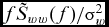
high-frequency spectral decay limit of $f{\tilde S_{ww}}( f )/\sigma _w^2$ (similarly for A_v and A_u) according to Kolmogorov's –5/3 Law

f

frequency (cycle/s or Hz)

${\tilde R_{ww}}$

modelled series expansion of autocorrelation of turbulence velocity w, (similarly for u and v)

R_wworR_wPwP

autocorrelation of vertical turbulence velocity w at a generic point P, first term in the perturbation series expansion of ${\tilde R_{ww}}$, a form of the von Karman vertical correlation function (similarly for R_uu and R_vv)

R_wPwQ

cross-correlation between vertical turbulence velocities at P and Q (similarly for u and v)

${\tilde S_{ww}}$

modelled series expansion of autospectrum of turbulence velocity w, (similarly for u and v)

S_wworS_wPwP

autospectrum of vertical turbulence velocity w at P (similarly for u and v)

S_wPwQ

cross-spectrum between vertical turbulence velocities at P and Q (similarly for u and v)

S^c _wPwQ,S _wPwQ^q

co-spectrum and quad-spectrum between vertical turbulence velocities at P and Q (similarly for u and v)

T_u,T_v and T_w

time scales of longitudinal, lateral, and vertical turbulence

t

time (s)

$\bar u,\ \bar v$and $\bar w$

mean turbulence velocities in the longitudinal, lateral, and vertical directions

u,v and w

turbulence velocities in the longitudinal, lateral, and vertical directions (see Fig. 1)

α_u,α_v, and α_w

scaling or normalisation parameters for autocorrelations (autospectra) of u,v, and w

β_1w,β_2w,. . ., β_nw

constants in the perturbation series expansion of ${\tilde R_{ww}}\ $ (see Equation (2a), similarly for ${\tilde R_{uu}}$ and ${\tilde R_{vv}}$)

γ²_wPwQ

coherence or coherence function between vertical turbulence velocities w ₁ at P and w ₂ at Q (similarly for γ²_uPuQ and γ²_vPvQ)

θ_wPwQ

phase angle of cross-spectrum ${\tilde S_{wPwQ}}$ (similarly for θ_uPuQ and θ_vPvQ)

σ_w

root mean square (rms) of vertical turbulence velocity (similarly for σ_u and σ_v)

σ²_w

variance or energy of vertical turbulence velocity (see Equation (2c), similarly for σ²_u and σ²_v)

τ

time interval or time lag, t ₂ - t _1,

2.0 MODEL STRENGTHS AND WEAKNESSES

Airwake-downwash turbulence deviates appreciably from ABL, whereas the framework is based on a perturbation-type series expansion in which the first term is represented by a form of the von Karman autocorrelation function from classical turbulence theory, including Taylor's hypothesis^{(Reference Gaonkar1)}. Moreover, there is no guarantee that the contribution of the first term of the series dominates over those of the second and remaining terms. These concerns should be tempered with the intended role of the framework: To provide a foothold on airwake-downwash phenomenon for engineering analysis. Moreover, the framework does not follow the classical perturbation theory approach of a linearised solution with perturbation corrections as add-ons. In fact, it represents a practical combination of series expansion, exploitation of the database, and theoretical constraints, and thereby it guarantees that time scale, mean square value and asymptomatic decay of the autospectral data points are preserved in the extracted models. It is emphasised that Taylor's hypothesis and the Kolmogorov –5/3 Law are found to be remarkably robust^{(Reference Mathieu and Scott11,Reference Townsend12)} . It is further emphasised that Taylor's hypothesis is not restricted to homogeneous turbulence and that this hypothesis is applicable to all turbulent flows as long as mean flow velocity is larger, compared to the eddy convection velocity^{(Reference Mathieu and Scott11,Reference Townsend12)} . “Thus, in practice, although Taylor's hypothesis is not exact, because real turbulence evolves as it is convected, it is approximately true in many flows^{(Reference Mathieu and Scott11)}.” While the validity of Taylor's hypothesis for airwake-downwash turbulence may be debatable, this hypothesis provides a powerful means of converting spatial coordinates into temporal coordinates. And the Kolmogorov –5/3 Law is well supported by experiments in a variety of flow fields, ranging from tidal flows and atmosphere near the sea surface to wind-farm wake turbulence and ship airwake with and without downwash^{(Reference Schau5,Reference Mathieu and Scott11)} . This Law requires, though, high-Reynolds-number and fully-developed-turbulence conditions^{(Reference Mathieu and Scott11)}. By design, the construction of shaping filters driven by white noise is as routine as the currently used procedure for the von Karman. What is more, the framework's utility is well borne out when tested against a comprehensive CFD database (details to follow). As things turn out, these models typically require no more than a first-order correction (a two-term series).

These weaknesses notwithstanding, this work should serve as a reference point for future investigations of downwash effects on the helicopter-ship dynamic interface. After all, almost all aspects of this interface, from pilot workload to excitations to the rotor/fuselage system to health and safety concerns, are affected by downwash coupling with airwake, not to mention the launch and recovery envelope^{(Reference Zan10)}.

3.0 DOWNWASH-IMPACT STATISTICS

The stochastic description is based on one-point statistics of autospectrum and two-point statistics of cross-spectrum and coherence. These statistics for airwake with downwash are compared with the corresponding statistics for airwake alone, and this comparison is used to quantify the impact of downwash on airwake. For all these results, the database lays the groundwork. Accordingly, it is presented first.

3.2 One-Point and Two-Point Statistics

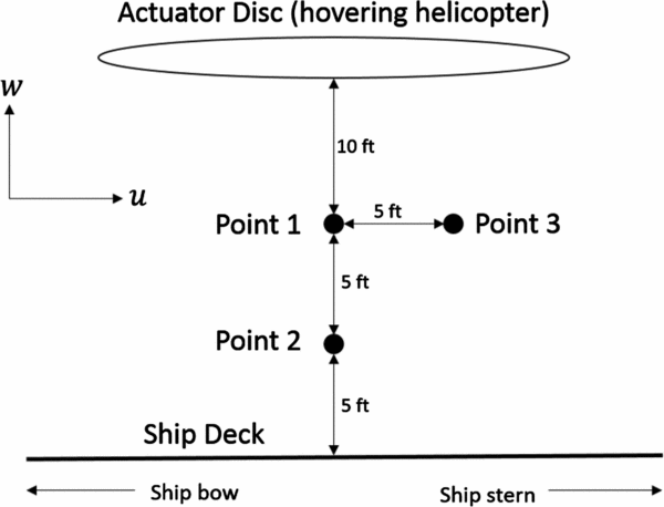
Given the extent of the database, the statistics are presented for three points in the spatial grid, which are schematically shown in Fig. 1, along with the topology relative to the actuator disk and landing deck. The first two points are 10 feet and 15 feet vertically below the actuator disk, and the third point is 5 feet horizontally to the right from the first. In the sequel, these three points are referred to as ‘Point One’, ‘Point Two’, ‘Point Three’, and the actuator disk is referred to as a “hovering helicopter”.

Figure 1.

A schematic of topology of point one, point two, and point three in the spatial grid relative to the actuator disk and deck level.

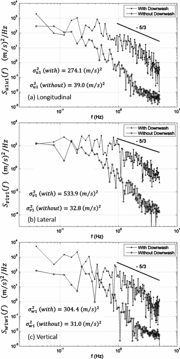
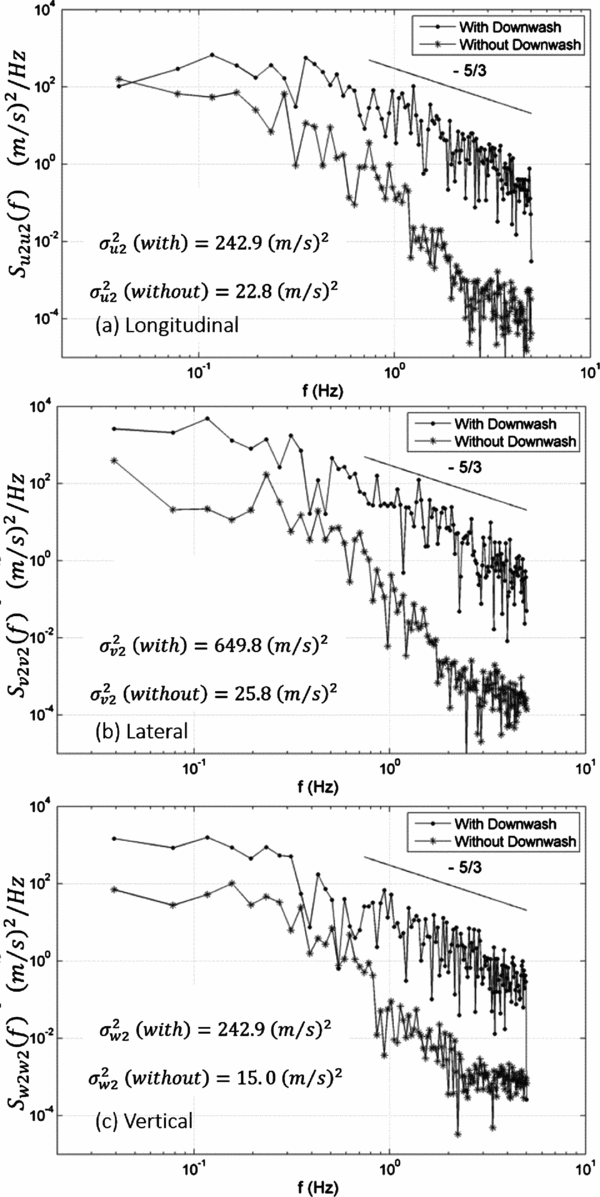
Figure 2 refers to Point One, and Fig. 3 to Point Two, 10 feet and 15 feet vertically below a hovering helicopter, respectively. Each of two figures presents how the autospectra of longitudinal, lateral, and vertical components for airwake with downwash compare with the corresponding autospectra for airwake alone. This comparison is of significance in that the area under dimensional S_ii(f) versus f curve represents the mean square σ²_i, which is also referred to as turbulence energy in the sense that σ²_i also represents variance (because the mean flow is subtracted from the velocity time history). Moreover, the frequency bandwidth over which this energy is concentrated can be identified as well. For illustration, the vertical component at Point One in Fig. 2 is considered. The energy, or mean squareσ²_W1, is31.00(m ²/s ²) without downwash, compared to 304.4(m ²/s ²), with downwash, nearly a tenfold increase due to downwash coupling. Equally important, almost all of this energy is concentrated within the low-frequency bandwidth (0.16 ⩽ f(Hz) ⩽ 1.6) that is of concern to helicopter flight mechanics. The results of Fig. 3 exhibit the same pattern, that is, one order of magnitude increase of turbulence energy because of downwash coupling: σ²_W2 = 242.9(m ²/s ²)with downwash compared to 15.00(m ²/s ²) without downwash, nearly a 16-fold increase (the autospectral and mean square results for Point Three (Fig. 1) essentially depict the same trend and are thus omitted).

Figure 2.

Autospectra with and without downwash at point one, 10 feet vertically below a hovering helicopter.

Figure 3.

Airwake autospectra with and without downwash at point two, 15 feet vertically below a hovering helicopter.

Compared to the preceding consideration of airwake-downwash turbulence energy and its concentration over a low-frequency bandwidth, the asymptotic decay of autospectra is more subtle. And, it is equally significant from the consideration of whether the turbulence flow field is still distorting or close to be being fully developed. As seen from Figs. 2 and 3, the asymptotic decay rate for all three velocity components of airwake with downwash is a bit higher than the Kolmogorov –5/3 decay rate, and for airwake alone, the decay rate is fairly comparable to the Kolmogorov rate. Observe that the Kolmogorov Law of –5/3 autospectral asymptomatic decay requires high-Reynolds-number and fully developed turbulence. Thus, this steeper-than-the-Kolmogorov decay rate due to downwash coupling seems to indicate that, compared to airwake alone, airwake with downwash is relatively less fully developed; that is, the eddy distortions are more pronounced and they continue longer. These remarks on the Kolmogorov decay rate, however, merit revisiting on the basis of experimental, at-sea or wind-tunnel data.

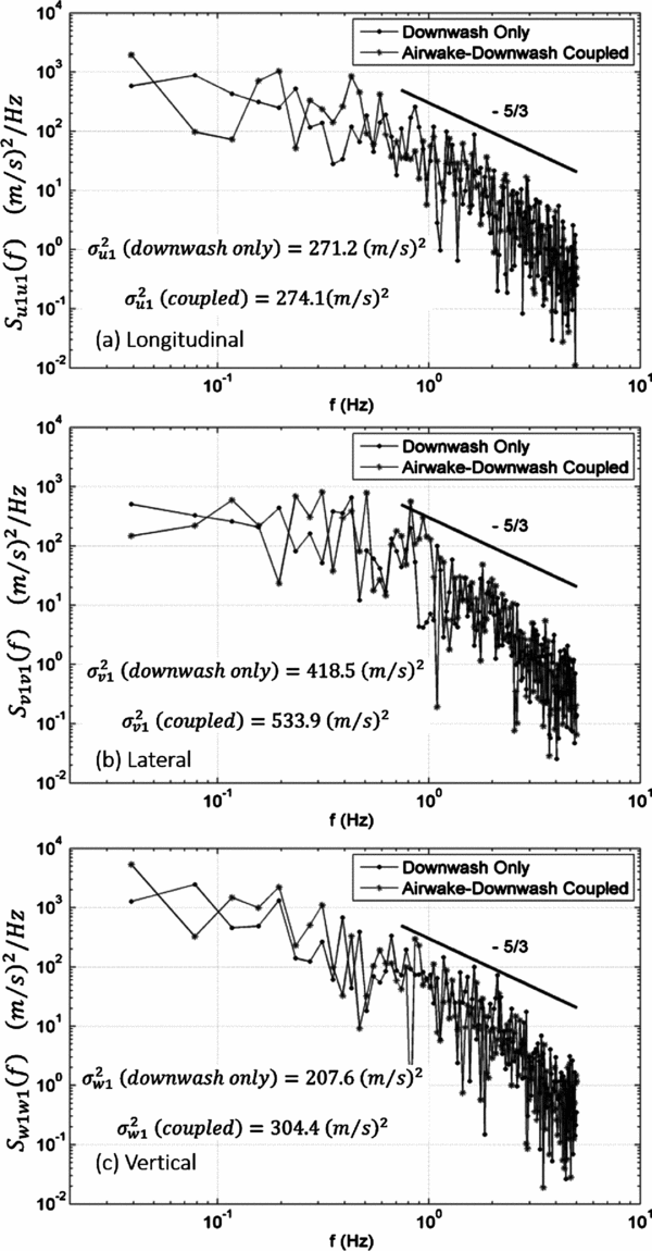
Figures 2 and 3 show the impact of downwash on the airwake flow field. The CFD database offers a set of data in which airwake is not present in the flow field, leaving downwash as the driving factor. Figure 4 shows the autospectral results from this downwash-only flow field at Point One, plotted with the coupled autospectra of Fig. 2. As expected, downwash is the driving factor in that the two spectra are virtually indistinguishable. Here as well, further research is required on the basis of experimental data.

Figure 4.

Airwake-downwash autospectra and downwash-only autospectra at point one, 10 feet vertically below a hovering helicopter.

The next set of statistics on the impact of downwash on airwake represents the two-point statistics of cross-spectrum and coherence. To help present the results without any ambiguities of terminologies, and to appreciate the results, the basic equations of the two-point statistics of cross-spectrum and coherence are first mentioned in passing, and then the results are presented. The correlation between, say vertical component w ₁(t) at Point One and w ₂(t + τ) at Point Two, for the time interval τ is the cross-correlation R _w1w2(τ). The Fourier transform of R _w1w2(τ) is the cross-spectrum, which is a complex valued function^{(Reference Bendat and Piersol13)}:

(1a)$$\begin{equation} {S_{w1w2}}\left( f \right) = \ S_{w1w2}^c\left( f \right) - i\ S_{w1w2}^q\left( f \right) = \left| {{S_{w1w2}}\left( f \right)} \right|\ {e^{ - i{\theta _{w1w2}}}}, \end{equation}$$

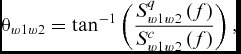
where S^c _w1w2(f) is the co-spectrum,S^q _w1w2(f) is the quad-spectrum, and θ_w1w2 is the phase angle. Specifically, the magnitude and phase are given by

(1b)$$\begin{equation} \left| {{S_{w1w2}}\left( f \right)} \right| = \sqrt {{{\left[ {S_{w1w2}^c\left( f \right)} \right]}^2} + {{\left[ {S_{w1w2}^q\left( f \right)} \right]}^2}},\\ \end{equation}$$

(1c)$$\begin{equation} {\theta _{w1w2}} = {\tan ^{ - 1}}\left( {\frac{{S_{w1w2}^q\left( f \right)}}{{S_{w1w2}^c\left( f \right)}}} \right), \end{equation}$$

Given the autospectra for both w ₁(t) and w ₂(t) – S _w1w1(f) and S _w2w2(f) – and the magnitude of the cross-spectrum between w ₁(t) and w ₂(t) – |S _w1w2(f)| – the corresponding coherence or coherence function (also referred to as the spectral correlation coefficient) is given by^{(Reference Bendat and Piersol13)}

(1d)$$\begin{equation} \gamma _{w1w2}^2\left( f \right) = \frac{{{{\left| {{S_{w1w2}}\left( f \right)} \right|}^2}}}{{{S_{w1w1}}\left( f \right){S_{w2w2}}\left( f \right)}}\ \ \,\ \ \ \ 0 \le \gamma _{w1w2}^2\left( f \right) \le 1 \end{equation}$$

As expected, forw ₁(t) = w ₂(t), γ²_w1w2(f) = 1 represents perfect correlation. Coherence γ²_w1w2(f) is greater than zero and less than one, and this shows the extent to which these two series are “similar” or correlated at each frequency.

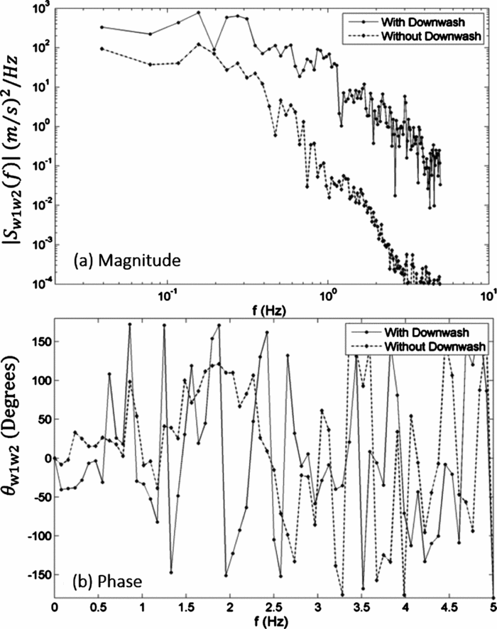
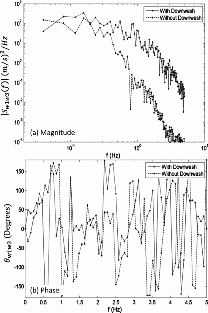
For both airwake and airwake-downwash turbulence, Fig. 5 shows the cross-spectrum S _w1w2(f) between the vertical components w ₁(t) at Point One and w ₂(t) at Point Two; magnitude, as typified by Equation (1b), is shown in Fig. 5(a), and phase, as typified by Equation (1c), in Fig. 5(b). As seen from Fig. 5(a), downwash impact on airwake is severe for both points; that is, airwake-downwash turbulence within the area containing both points has more energy than airwake for the entire frequency range. The phase information in Fig. 5(b) is extremely instructive in comparison to some of the extensively pursued nonhomogeneous, anisotropic flow fields. As an illustration, for ABL near the ground, the phase angle is found to be relatively small and thus, the cross-spectrum is often approximated by the real part or co-spectrum; see Reference Simiu and ScanlanRef. 14 for details. By contrast, Fig. 5(b) shows that, for both airwake and airwake-downwash turbulence, the widely used small-phase approximation, that is, approximating cross-spectrum by its real part co-spectrum, is not tenable. For a relatively complete picture of two-point statistics in the interface, the cross-spectrum between point one and point three – S _w1w3(f) – is also included in Fig. 6, magnitude in Fig. 6(a), and phase in Fig. 6(b). Here as well, the overall impact of downwash on airwake on the basis of cross-spectrum magnitude and phase variation with frequency is similar to that of S _w1w2(f) in Fig. 5. The cross-spectral results for the longitudinal and lateral components are essentially similar to those of the vertical components and are thus omitted.

Figure 5.

Airwake vertical cross-spectrum with and without downwash between point one and point two (these two points are identified in Fig. 1).

Figure 6.

Airwake vertical cross-spectrum with and without downwash between point one and point three (these two points are identified in Fig. 1).

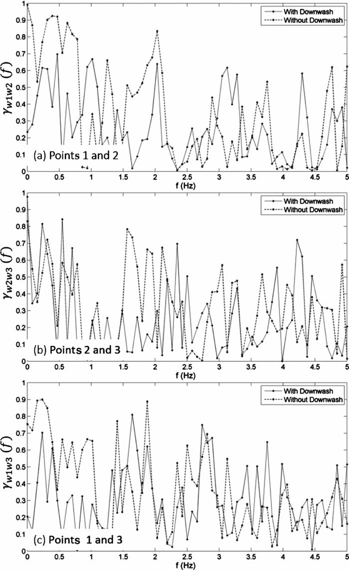
Figure 7 shows coherences γ²_w1w2(f), γ²_w1w3(f), and γ²_w2w3(f) for vertical velocity components for three pairs of points; also see Fig. 1. For example, γ²_w1w2(f) represents the dimensionless correlation between vertical components w ₁(t) at Point One and w ₂(t) at Point Two in the frequency domain; this should explain why coherence, as typified by Equation (1d), is also referred to as the spectral correlation coefficient. Coherence is widely used as a quantitative measure of similarity (or dissimilarity) between two time histories of flow velocities^{(Reference Bendat and Piersol13)}. As seen from Fig. 7, for airwake-downwash turbulence, the coherence is generally low (sayγ²_ii < 0.5) for all three velocity components for most of the entire bandwidth(0 ⩽ f(Hz) ⩽ 5); this indicates that the two time histories of the corresponding components at these two points are weakly correlated. By comparison, the coherence values are much higher (γ²_ii > 0.5) for airwake alone; that is, the correlation between the corresponding time histories is relatively stronger. These comparative features are consistent with the physics of two flow fields. Compared to airwake, airwake-downwash turbulence is far more distorting with reduced point-to-point similarity because of downwash coupling.

Figure 7.

Vertical airwake coherences with and without downwash for three pairs of points (these three points are identified in Fig. 1).

As seen from Fig. 1, all three points, thus far investigated, are below the rotor plane, two points vertically down and the third one slightly behind the rotor. Although significant in the prediction of downwash-induced fuselage loads and the corresponding impact on pilot work load and operational envelope^{(Reference Lee and Zan9,Reference Zan10)} , flow disturbances at these below-the-rotor-plane points represent an excitation that is internal to the rotor-fuselage system: from the rotor to the fuselage. By comparison, flow disturbances at points upstream of the rotor and above the rotor plane convect downstream and directly impact the rotor as an excitation to the rotor itself; and this excitation is thought to have a major effect on low-speed helicopter flight dynamics. That is, this excitation (rather than fuselage forces) is the primary source of pilot workload and limitations. Accordingly, one point just upstream of the rotor, and two points above the rotor are selected (these points are not shown). Specifically, the upstream point is on the rotor plane and 10feet forward of the rotor, and the other two points are 5feet and 10feet vertically above the rotor. For quantitative illustration, suffice it to consider σ²_w, the energy values of the vertical components of airwake alone and airwake with downwash. Because of downwash, σ²_w increases threefold at the point 5feet vertically above, and 40% at the upstream point on the rotor plane and marginally at the point 10feet vertically above. Finally, it is also instructive to compare downwash effects at two “representative points” that are above and below the rotor plane, say at Point One (Fig. 1), 10feet vertically below the rotor and at another point, 5feet vertically above. At Point One, σ²_w increases tenfold from downwash and at the latter point, it increases threefold. The message is that, while downwash effects vary from point to point, these effects should be included in any realistic assessment of how the flow-field affects the vehicle.

4.0 MATHEMATICAL FRAMEWORK

The mathematical framework represents the series expansion approach in combination with the theoretical constraints and a database so that the extracted autospectral model from this database and the autospectral data points have the same time scale, mean square value, and asymptotic decay. The contributions of this paper are novel in three respects: (1) Derivation of theoretical constraints of time scale and asymptotic decay in closed form for the vertical component (essentially the same constraints apply to the lateral component with minor changes); (2) Development of a framework with built-in theoretical constraints for all three components (the constraints for the longitudinal were derived earlier by Harris^{(Reference Harris6)}); and (3) Demonstration of the framework's viability against a comprehensive database.

For illustration, the vertical velocity component w(t) of airwake-downwash turbulence is selected; therein, the mean value $\bar w( t )$ plus the corresponding fluctuation or turbulence w(t) represent the total vertical component: $w( t ) + \ \bar w( t ).$ For the longitudinal and lateral components, the details run virtually parallel to those of the vertical. Moreover, for helicopter flight dynamics applications, the vertical component is generally more important than the other two components.

4.1 Vertical Turbulence Model

The autocorrelation of vertical airwake-downwash turbulence ${\tilde R_{ww}}( \tau )$ is expressed by a perturbation-type series:

(2a)$$\begin{equation} {\tilde R_{ww}}\left( \tau \right) = {\beta _{1w}}{R_{ww}}\left( \tau \right) + {\beta _{2w}}R_{ww}^2\left( \tau \right) + \cdots + {\beta _{nw}}R_{ww}^n\left( \tau \right)\ \ \end{equation}$$

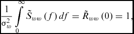
Using the classical definition of time scale ${T_w} = \mathop \smallint_0^\infty {\tilde R_{ww}}( \tau )d\tau $ and with ${\tilde S_{ww}}( f )$ representing the vertical airwake-downwash turbulence autospectrum, Equations (2b) and (2c) provide the footholds for the derivation of the constraint equations.

(2b)$$\begin{equation} {\tilde S_{ww}}\left( 0 \right) = 4\sigma _w^2\mathop \int\limits_0^\infty {\tilde R_{ww}}\left( \tau \right)d\tau = 4\sigma _w^2{T_w},\\ \end{equation}$$

(2c)$$\begin{equation} \frac{1}{{\sigma _w^2}}\mathop \int\limits_0^\infty {\tilde S_{ww}}\left( f \right)df = {\tilde R_{ww}}\left( 0 \right) = 1, \end{equation}$$

where σ²_W is the mean square value, or variance. Furthermore,R_ww(τ), the first term on the right side of Equation (2a), is referred to here as a basis function, and it is represented by a form of the von Karman vertical correlation function:

(2d)$$\begin{equation} {R_{ww}}\left( \tau \right) = \frac{{{2^{2/3}}}}{{{\rm{\Gamma }}\left( {\frac{1}{3}} \right)}}{\left( {\frac{{{\alpha _w}\tau }}{{{T_w}}}} \right)^{1/3}}\left[ {{K_{1/3}}\left( {\frac{{{\alpha _w}\tau }}{{{T_w}}}} \right) - \frac{1}{2}\left( {\frac{{{\alpha _w}\tau }}{{{T_w}}}} \right){K_{2/3}}\left( {\frac{{{\alpha _w}\tau }}{{{T_w}}}} \right)} \right], \end{equation}$$

where α_w is introduced to satisfy Equation (2b) and serves as a time-scale preservation parameter. K _1/3 and K _2/3 are modified Bessel functions of order 1/3 and 2/3, respectively; this is necessitated by the definition of autocorrelation, ${\tilde R_{ww}}( 0 ) = 1$, regardless of the value of α_w. As seen from Equations (2a) and (2d), β_1w,β_2w,. . ., β_nw along with α_w, represent n+1 unknown constants. Their evaluation requires the autospectrum, which is obtained by taking the Fourier transform of Equation (2a):

(3)$$\begin{equation} {\tilde S_{ww}}\left( f \right) = {\beta _{1w}}{S_{ww1}}\left( f \right) + {\beta _{2w}}{S_{ww2}}\left( f \right) + \cdots + {\beta _{nw}}{S_{wwn}}\left( f \right), \end{equation}$$

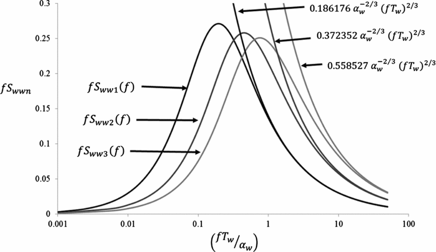
where S_wwn(f) is the Fourier transform of Rⁿ_ww(τ). A part of Fig. 8 shows the corresponding Fourier transforms multiplied by f: fS _ww1(f), fS _ww2(f), and fS _ww3(f) (i.e. the terms of Equation (3) if all beta coefficients are set to unity).

Figure 8.

A geometrical representation of asymptotic decay according to the Kolmogorov –5/3 law.

4.2 Constraint Equations

Since ${\rm{\ }}{\tilde R_{ww}}( 0 ) = {R_{ww}}( 0 ) = 1$, Equation (2a) gives

(4a)$$\begin{equation} {\beta _{1w}} + {\beta _{2w}} + \cdots + {\beta _{nw}} = 1\ \ \end{equation}$$

Integrating Equation (2a), and using the relation in Equation (2b) lead to^{(Reference Schau5)}:

(4b)$$\begin{equation} {\alpha _w} = {\beta _{1w}}\mathop \int\limits_0^\infty {R_{ww}}\left( \tau \right)d\tau + {\beta _{2w}}\mathop \int\limits_0^\infty R_{ww}^2d\tau + \cdots + {\beta _{nw}}\mathop \int\limits_0^\infty R_{ww}^nd\tau \\ \end{equation}$$

(4c)$$\begin{equation} {\alpha _w} = \frac{{\sqrt \pi {\rm{\Gamma }}\left( {\frac{5}{6}} \right)}}{{2{\rm{\ \Gamma }}\left( {\frac{1}{3}} \right)}}\left[ {{\beta _{1{\rm{w}}}} + {\beta _{2{\rm{w}}}}\frac{{79\sqrt 3 }}{{256}} + {\beta _{3w}} \times D} \right], \end{equation}$$

whereD is evaluated numerically. Finally,

(4d)$$\begin{equation} {\alpha _w} = 0.373417\,{\beta _{1w}} + 0.199591\,{\beta _{2w}} + 0.122360\,{\beta _{3w}} \end{equation}$$

Similarly, the Kolmogorov asymptotic Law requires^{(Reference Schau5)}:

(5a)$$\begin{equation} {\left[ {\frac{{f\ {S_w}\left( f \right)}}{{{\sigma _w}^2}}} \right]_{{\rm{high}}\ {\rm{frequency}}}} = {A_w}{\left( {f\ {T_w}} \right)^{ - 2/3}} \end{equation}$$

After some manipulations, Equation (5a) reduces to

(5b)$$\begin{equation} \frac{{{A_w}}}{{\alpha _w^{2/3}}} = \frac{{16}}{{3{{\left( {2\pi } \right)}^{5/3}}}}\frac{{\sqrt \pi {\rm{\ \Gamma }}\left( {\frac{5}{6}} \right)}}{{{\rm{\Gamma }}\left( {\frac{1}{3}} \right)}}\left[ {{\beta _{1w}} + 2{\beta _{2w}} + 3{\beta _{3w}} + \cdots } \right], \end{equation}$$

where A_w is the asymptotic value, which is extracted from the autospectral data points according to Equation (5a)^{(Reference Schau5)}. This equation is simplified to:

(5c)$$\begin{equation} \frac{{{A_w}}}{{\alpha _w^{2/3}}} = \ 0.186176\,{\beta _{1w}} + 0.372352\,{\beta _{2w}} + 0.558527\,{\beta _{3w}} \end{equation}$$

Figure 8 shows a geometrical representation of Equation (5c); for additional details, see Reference SchauRef. 5. The closed form expressions, as typified by Equations (4a), (4c), and (5b), represent the constraint equations of the model framework.

5.0 NUMERICAL ASPECTS

The process of managing the voluminous database and generating the autospectral data points, and then evaluating the unknowns in the series expansion, involves many and varied details^{(Reference Schau5)}. The following account is intended to convey a flavor of this process; although addressed for the vertical component, it applies to the other two components as well. As seen from Equations (2a) and (2d), the numerical task boils down to computing ‘n’ series-expansion constants of β_1w,β_2w,β_3w, and one normalisation parameter α_w. The task begins with the evaluation of the mean square value σ²_w directly from the raw data points. Then, the autospectral data points, including the point at zero frequency, are generated from the database, and the mean square value σ²_w is once again evaluated from Equation (2c); these two sets of mean square values are found to agree fairly well. Finally, the time scale T_w is calculated from Equation (2b), and the asymptotic limit A_w is graphically evaluated from Equation (5a).

Having thus extracted time scale T_w and asymptotic limit A_w from the database, the numerical scheme now turns to solving for n+1 unknowns – β_1w,β_2w,β_3w, along with α_w – and to subjecting this solution to satisfy the constraints typified by Equations (4a), (4d), and (5c). As seen from Equation (4d), these n β-coefficients completely determine α_w, not the other way around. Thus, the numerical scheme actually involves the computation of n β-coefficients that satisfy the two constraints given by Equations (4a) and (5c).

Throughout, the constraint given by Equation (4a) is strictly enforced, and the numerical scheme begins with the von Karman model: β_w = 1. The optimisation algorithm ‘sqp’ subjected to the constraints detailed above is used to minimise the error between the n β-coefficients of the model and the autospectral data points. When the β coefficients alone are considered without any reference to the asymptotic constraint A_w of Equation (5c). (Recall that Equation (4a) is always enforced), the minimisation process leads to several solutions sets, with minor differences between any two solution sets (e.g. these minor differences are due to the differences in the selection of the autospectral data points.)

When the β coefficients are considered along with the A_w constraint of Equation (5c), the numerical scheme becomes demanding in that it may lead to one set of β-coefficients thus satisfying all the constraints exactly but the β-coefficients may not adequately fit the data. Accordingly, an alternative numerical scheme is devised: A least-squares minimisation of the sum of the errors between the β-coefficients and the autospectral data points and between the A_w coefficient of the model (resulting from the β-coefficients, see Equation (5c)) and the measured A_w. This alternative scheme is found to be remarkably robust and routine, and the computed A_w values are generally found to be within 3%.

6.0 AIRWAKE-DOWNWASH MODELS

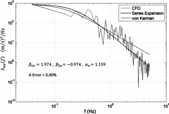
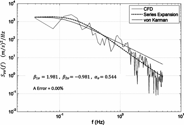
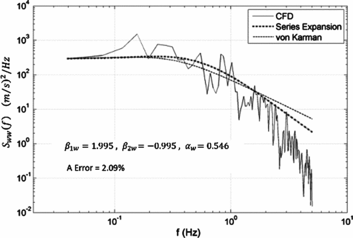
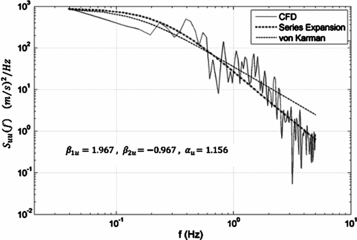
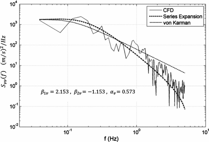
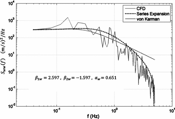
The framework is tested against a comprehensive database of airwake-downwash turbulence^{(Reference Schau5)}. A representative sample of the results from this testing is now presented in Figs. 9-14. Therein, the extracted interpretive models of autospectra are compared with the numerically generated autospectral data points from the database and the von Karman models (e.g. β_1u = 1 for the longitudinal component).

Figure 9.

Longitudinal autospectra of airwake-downwash turbulence from CFD, von Karman, and two-term series expansion.

Figure 10.

Lateral autospectra of airwake-downwash turbulence from CFD, von Karman, and two-term series expansion.

Figure 11.

Vertical autospectra of airwake-downwash turbulence from CFD, von Karman, and two-term series expansion.

Figure 12.

Longitudinal autospectra of airwake-downwash turbulence from CFD, von Karman, and two-term series expansion, without the a-constraint.

Figure 13.

Lateral autospectra of airwake-downwash turbulence from CFD, von Karman, and two-term series expansion without the A-constraint.

Figure 14.

Vertical autospectra of airwake-downwash turbulence from CFD, von Karman, and two-term series expansion without the A-constraint.

For a segment of the database, the autospectral data points are found to exhibit a mixed trend: for some velocity components, the Kolmogorov –5/3 Law was clearly exhibited, while for the other components, this Law was not so clearly exhibited. Accordingly, for the same set of autospectral data points, the framework is used with the enforcement of the Kolmogorov Law in Figs. 9-11, and without this enforcement, in Figs. 12-14. Moreover, in Figs. 9-11, “A Error = xx %” indicates the error in satisfying the Kolmogorov –5/3 Law. As it turns out, rigorous enforcement of Equation (5c) severely limits the model. Due to the nature of the –5/3 law, allowing the model's asymptotic decay level to deviate from the measured value is acceptable. An error of less than 10% is considered acceptable for engineering analysis. To clarify the previous statement: The beta coefficients of Equation (3) are solved for in a least squares (curve fitting) sense, with exact adherence to the constraint Equation (4a). To allow for a greater set of possible solutions, Equation (5c) is enforced to within an acceptable level. Similarly, in Figs. 12-14, “without the A-Constraint” means that the asymptotic decay according to the Kolmogorov –5/3 Law typified by Equation (5c), is not enforced. Now, the least-squares solution is subjected to two constraints, typified by Equations (4a) and (4d). Another point merits mention: The selection of a specific segment of the database with a mixed trend of exhibiting the Kolmogorov –5/3 Law is intentional. Its purpose is to demonstrate that the framework lends itself remarkably well to a wide range of the database, irrespective of whether the autospectral data points exhibit the Kolmogorov –5/3 Law or not. Ignoring Equation (5c) in the model extraction is completely appropriate, if the data itself does not exhibit the –5/3 Law.

As seen from all these six figures, Figs. 9-14, the developed models with only a first-order correction (a two-term series) approximate the autospectral data points remarkably well, and they represent a significant improvement over the von Karman model.

It is also instructive to compare the extracted models with the –5/3 Law enforcement to those without the enforcement. For the longitudinal and lateral components (Figs. 9, 12 and Figs. 10, 13, respectively), the autospectral data points exhibit asymptotic decay according to the –5/3 Law, and enforcement of this Law is found to be desirable. Specifically, for the longitudinal component, both cases with and without the enforcement lead to virtually identical models, and for the lateral component, the model with the enforcement better approximates the autospectral data points; for example, compare Figs. 10 with 13, in particular, for frequencies greater than 1Hz.

For the vertical component in Figs. 11 and 14, the autospectral data points exhibit a steeper-than-the –5/3 slope. In this case, the model without this enforcement (Fig. 14) represents a qualitative improvement over the model with the enforcement (Fig. 11). The reason is that the enforcement hinders the framework's capability for the model extraction for the flow-field at this particular location.

In summary, these six figures demonstrate that the framework is remarkably robust: The capability for extracting autospectral models from a wide range of autospectral data points with and without the Kolmogorov –5/3 asymptotic decay. They further demonstrate that, with only a first-order correction, the framework extracts models that provide an excellent approximation of the autospectral data points, and a vast improvement over the von Karman. It is important to note that although the points modelled are below the rotor, they could be applied to any point in the flow field, for example, above and upstream of the rotor.

7.0 SIMULATION FILTERS

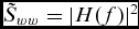
For the one-point statistics of autospectrum (e.g. ${\tilde S_{ww}}( f )$ in Equation (3)), simulation requires reconstruction of the random process or time histories from the extracted autospectral models. Accordingly, random white noise is passed through a filter, a single-input single-output system, say with system function H(f). Since white noise autospectrum is constant, it is set to unity, and now, the response autospectrum of the shaping filter is simply |H(f)|². Thus, the random process reconstruction simplifies to designing a shaping filter with system function H(f) such that |H(f)|² agrees with the extracted autospectrum model; that is, ${\tilde S_{ww}} = {| {H( f )} |^2}$.

A key feature of the extracted autospectrum models of airwake-downwash turbulence, as typified in Equation (3), is that the filter design is virtually identical to the widely-used design for the von Karman autospectra. For the vertical autospectrum, the system function for the extracted autospectrum models can be expressed as^{(Reference Schau5)}:

(6)$$\begin{equation} \frac{{{H_w}\left( f \right)}}{{{\sigma _W}}} = \frac{{4\sqrt {{T_W}} \ \left( {1 + {b_1}{T_W}f + {b_2}{{\left( {{T_W}f} \right)}^2}} \right)}}{{1 + {a_1}{T_W}f + {a_2}{{\left( {{T_W}f} \right)}^2} + {a_3}{{\left( {{T_W}f} \right)}^3}}} \end{equation}$$

In the above equation, T_W is time scale, referred to earlier in Equation (2b). The time scale is calculated from the data. The remaining five coefficients – a₁, a₂, a₃, b₁ and b₂ – are evaluated by nonlinear data fitting to the extracted autospectral model on a least squares basis^{(Reference Schau5)}.

7.1 Airwake-Downwash Simulation

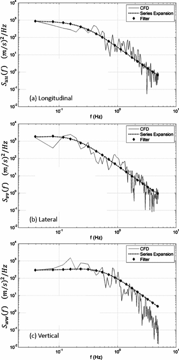
The filter design follows Equation (6), and Fig. 15 shows how the autospectra from these white-noise-driven filters compare with the autospectral data points and with the extracted models from the database. These autospectral data points and the extracted models are identical to the models presented earlier in Figs. 9-11. The extracted models are found to lend themselves extremely well to the design of filters^{(Reference Schau5)}, and, as seen from Fig. 15, they agree well with the other two sets of models: autospectral data points (CFD) and extracted interpretive model (series expansion).

Figure 15.

Airwake-downwash turbulence autospectra from CFD, two-term expansion series, and shaping filter simulation of two-term series model.