
1. Introduction
The motion of a flexible film/filament in the wake of a bluff body is the quintessence of flow–structure interactions. Copious phenomena of biological undulatory locomotion, such as the rainbow trout (Oncorhynchus mykiss) adopting Kármán gait in the vortex street behind an obstacle (Liao et al. Reference Liao, Beal, Lauder and Triantafyllou2003a,Reference Liao, Beal, Lauder and Triantafylloub), the trailing fish swimming in the vortex wake generated by the preceding two side-by-side fish in a diamond formation (Weihs Reference Weihs1973; Liao Reference Liao2007) and the larval zebrafish (Danio rerio) or tadpole whipping the tail to propel in streams (Van Buskirk & McCollum Reference Van Buskirk and McCollum2000; Wang et al. Reference Wang, Ren, Hu, Li and Sitti2021), can be abstracted as the interactions between the flexible film and the periodic vortices.
Both laboratory experiments and field observations have revealed that fish exhibit a preference for swimming in the wake flow of an obstacle (e.g. the rock in the natural river or the cylinder vertically placed in the uniform flow in the experiment) as they moved against the current (Liao Reference Liao2007). It is believed that in the wake flow of a bluff body where the periodic vortices prevail, fish can reduce their energy expenditure either by taking advantage of the low-pressure feature in the circulation region or by harnessing the energy from the oncoming periodic vortices (Beal et al. Reference Beal, Hover, Triantafyllou, Liao and Lauder2006; Liao Reference Liao2007; Taguchi & Liao Reference Taguchi and Liao2011; Ortega-Jiménez & Sanford Reference Ortega-Jiménez and Sanford2021). Two representative swimming states of a fish in the wake of a cylinder, contingent on the streamwise distance between the fish and the cylinder, are documented in the literature. When the fish enters the recirculation region with its head close but not against the cylinder, the undulation of the fish's body decreases drastically, and the fish performs irregular yawing flutter with a very small amplitude, which is designated as the ‘entraining state’ (Webb Reference Webb1998; Liao Reference Liao2006; Przybilla et al. Reference Przybilla, Kunze, Rudert, Bleckmann and Brücker2010; Ortega-Jiménez & Sanford Reference Ortega-Jiménez and Sanford2021). This state is favourable for energy saving due to the small body flutter. When the fish swims in the periodic vortex street downstream of the cylinder, it synchronizes the body undulation with the vortex street in frequency and phase, and performs large lateral motion and bending. In this situation, the fish slaloms between the oncoming vortices without traversing or breaking them. This locomotion is termed the ‘Kármán gaiting’ state by Liao et al. (Reference Liao, Beal, Lauder and Triantafyllou2003a,Reference Liao, Beal, Lauder and Triantafylloub). Through this particular gait, fish exploit their interactions with the oncoming large-scale vortices to generate passive lateral body bending, thereby extracting energy from the vortices and reducing their metabolic costs (Beal et al. Reference Beal, Hover, Triantafyllou, Liao and Lauder2006; Liao Reference Liao2007; Taguchi & Liao Reference Taguchi and Liao2011).
The existing quantitative kinematic model for the Kármán gaiting describes the motion of the fish body as a linear superposition of the periodic translation, rotation and bending waves (Akanyeti & Liao Reference Akanyeti and Liao2013b). This model is merely capable of representing the primary morphological characteristics of the Kármán gaiting but powerless for more in-depth physical analyses, for example, solving the energy distribution, since the average deviation of the modelled motion from the fish's action attains 27.73 % (Akanyeti & Liao Reference Akanyeti and Liao2013b), while the maximum deviation is around 60 % (this value is assessed from the figure in that paper). Regarding the entraining state, the previous studies based on direct observations deemed it as an indiscernible pattern (Webb Reference Webb1998; Liao Reference Liao2007; Przybilla et al. Reference Przybilla, Kunze, Rudert, Bleckmann and Brücker2010), lacking quantitative description and analysis. Accordingly, it is imperative to develop quantitative methods to characterize the Kármán gaiting and the entraining state accurately. In both the Kármán gaiting and the entraining state, a remarkable fact is that the fish activates less muscle and behaves like a passive hydrofoil in the cylinder wake (Liao et al. Reference Liao, Beal, Lauder and Triantafyllou2003a; Müller Reference Müller2003; Taguchi & Liao Reference Taguchi and Liao2011; Tong, Xia & Chen Reference Tong, Xia and Chen2021). Consequently, the simplified model of the flow–structure interaction, i.e. a flexible film flaps or flutters in the wake of a circular cylinder, holds promise for providing inspirations for the physics underlying these systems. The motion of the film in the wake is entirely passive. This feature allows us to decipher how the fish passively harnesses energy from the vortex street or takes advantage of the unsteady flow in the wake of a bluff body, thus offering insights that may inspire energy-efficient motion strategies (Ristroph & Zhang Reference Ristroph and Zhang2008; Alben Reference Alben2012). More importantly, given the dynamic similarities among the different undulatory motions, the methods developed from the analyses of the film motion would find application in the broader field of piscine locomotion research.
In the abiotic realm of nature, as we mention the interaction between the flexible film and fluid flow, one may immediately associate it with a flag fluttering or flapping in the wind. The systematic research on flag dynamics dates from the mid-1960s, in which Taneda (Reference Taneda1968) completed a series of experiments in a vertical wind tunnel. He reported that the flag showed three typical motion states successively with the gradual increase of the free stream velocity, which were the flutter with a small amplitude, the regular periodic flapping and the violent irregular flapping, respectively. Taneda's results have led the orientation of the experimental and numerical researches over the past decades, in which the variety of motion states mentioned are still worthy of detailed investigations by later researchers (Shelley & Zhang Reference Shelley and Zhang2011). Another piece of impressive research is the simplified facsimile of the flag's two-dimensional motion via a silk thread in a gravity-driven soap-film flow by Zhang et al. (Reference Zhang, Childress, Libchaber and Shelley2000). They observed two different dynamical states: the stretched-straight and stable periodic flapping state. A special phenomenon was that the two states could be switched alternately with the action of external force. The periodic flapping of the flag has been verified to be well modelled as a travelling wave with a linearly increasing spatial envelope in streamwise orientation (Zhang et al. Reference Zhang, Childress, Libchaber and Shelley2000; Alben & Shelley Reference Alben and Shelley2008; Ristroph & Zhang Reference Ristroph and Zhang2008). The motion of the trailing edge of the flag induces shear flow in the wake flow field, resulting in a series of small-scale Kelvin–Helmholtz (K–H) vortex structures or alternately shed Kármán vortices, depending on the free stream velocity (Zhang et al. Reference Zhang, Childress, Libchaber and Shelley2000; Jia et al. Reference Jia, Li, Yin and Yin2007; Alben & Shelley Reference Alben and Shelley2008; Portaro et al. Reference Portaro, Fayed, Gunter, Abderrahmane and Ng2011). The states of a flexible film/flag in the flow field are dominated both by the flow parameters (free stream velocity  $U_\infty$, fluid density
 $\rho _f$) and by the material parameters of the film itself (material density
 $\rho _s$, streamwise length
 $L$, spanwise width
 $b$, thickness
 $h$ and bending stiffness
 $B$); these parameters yield two non-dimensional parameters that govern the coupling system between the flexible film and the flow field, namely the structure-to-fluid mass ratio
 $S$ and the effective bending stiffness
 $K_B$ as the following, respectively (Connell & Yue Reference Connell and Yue2007; Shelley & Zhang Reference Shelley and Zhang2011; Sader et al. Reference Sader, Cossé, Kim, Fan and Gharib2016),
 \begin{equation} S = \frac{\rho_s h}{\rho_f L}\quad \mathrm{and} \quad K_B = \frac{B}{\rho_f U_\infty^2 b L^3}.\end{equation}
In the two-dimensional parameter space spanned by  $S$ and
 $K_B$, each dynamical state of the flexible film corresponds to a specific point in the
 $S$–
 $K_B$ plane. We can implement the transition of the film from a stationary state to a flapping state by adjusting
 $S$ and
 $K_B$ and vice versa; then, we can identify a stability boundary (or instability boundary) by tracking all the parameter points
 $(S,K_B)$ at which the transition occurs (Argentina & Mahadevan Reference Argentina and Mahadevan2005; Connell & Yue Reference Connell and Yue2007; Jia et al. Reference Jia, Li, Yin and Yin2007; Alben & Shelley Reference Alben and Shelley2008; Pfister & Marquet Reference Pfister and Marquet2020). In addition, this stability/instability transition displays evident hysteresis (Zhang et al. Reference Zhang, Childress, Libchaber and Shelley2000; Eloy et al. Reference Eloy, Lagrange, Souilliez and Schouveiler2008; Eloy, Kofman & Schouveiler Reference Eloy, Kofman and Schouveiler2012). The film also transitions to intense, irregular, aperiodic flapping as the parameters
 $S$ and
 $K_B$ are manipulated (Connell & Yue Reference Connell and Yue2007; Alben & Shelley Reference Alben and Shelley2008; Michelin & Doaré Reference Michelin and Doaré2013; Shukla, Govardhan & Arakeri Reference Shukla, Govardhan and Arakeri2013), which means there may be a boundary that represents the transition from periodic state to aperiodic state but that remains to be revealed further. The attention paid to the aperiodic flapping of a film is currently insufficient, and the related studies are still in their infancy, leaving ample room for further exploration, crucially, developing quantitative methods to determine and portray the aperiodic flapping. It constitutes one of the interests of our present study.
In the previous studies on flag flapping, the coupling system was routinely simplified as the interaction between a flexible film and uniform flow, where the influence of the flagpole was neglected (Taneda Reference Taneda1968; Zhang et al. Reference Zhang, Childress, Libchaber and Shelley2000; Huang & Sung Reference Huang and Sung2010; Hœpffner & Naka Reference Hœpffner and Naka2011; Shelley & Zhang Reference Shelley and Zhang2011). The top diameter of a common flagpole is approximately 80 mm, according to which the Reynolds number attains  $Re\sim O(10^4)$ even in a breeze (with a speed of approximately
 $5\ \text {m s}^{-1}$). Hence, we must be conscious that large-scale vortices do shed periodically from the flagpole as the wind blows it (Williamson Reference Williamson1996); furthermore, the spatial scale of the periodic vortices exceeds the flagpole diameter and gradually grows whilst they convect downstream (Zdravkovich Reference Zdravkovich1996; Wang et al. Reference Wang, Gan, Xu and Zhou2020; Duan & Wang Reference Duan and Wang2021). Accordingly, a more cogent physical model for the coupling system of a flag flapping is posited on the interaction of a flexible film with the periodic vortices from a cylinder, which is more drastic and complex than the interaction with a uniform flow. This, in turn, implies the existence of complex and intensive energy exchange between the film and the flow field.
Actually, as an archetype of the flow–structure interaction, the motion of a flexible film in the cylinder wake has captivated many scholars. A series of investigations, encompassing experiments, numerical simulations and theoretical analyses, have been conducted to dig out the characteristics and mechanisms underlying this flow–structure interaction model. It has been revealed that an appropriately sized flexible film contributes to the reduction of drag (Lee & You Reference Lee and You2013; Sharma & Dutta Reference Sharma and Dutta2021; Mao, Liu & Sung Reference Mao, Liu and Sung2022), noise (Duan & Wang Reference Duan and Wang2021) and vibration (Sahu, Furquan & Mittal Reference Sahu, Furquan and Mittal2019; Cui, Feng & Hu Reference Cui, Feng and Hu2022) associated with flow over a circular cylinder or similar bluff bodies. However, a substantial number of fundamental issues related to this model are seemingly long shunned and thus demand urgent solution. The majority of investigations are predominantly performed by two-dimensional numerical simulations at pretty low Reynolds numbers (even at Reynolds numbers involving laminar vortex shedding), such as  $Re=100$ in Lee & You (Reference Lee and You2013),
 $Re=150$ in Wu et al. (Reference Wu, Qiu, Shu and Zhao2014),
 $Re=100\ {\rm and}\ 200$ in Kundu et al. (Reference Kundu, Soti, Bhardwaj and Thompson2017),
 $Re=150$ in Sahu et al. (Reference Sahu, Furquan and Mittal2019),
 $Re=80$ in Pfister & Marquet (Reference Pfister and Marquet2020),
 $Re=150$ in Furquan & Mittal (Reference Furquan and Mittal2021) and
 $Re=100$ in Mao et al. (Reference Mao, Liu and Sung2022), to name but a few, which are significantly smaller than the Reynolds number encountered by real-world flag flapping or fish swimming. Several noteworthy experiments with
 $Re\sim O(10^3)-O(10^5)$, including studies by Shukla et al. (Reference Shukla, Govardhan and Arakeri2013), Sharma & Dutta (Reference Sharma and Dutta2020, Reference Sharma and Dutta2021), Deng et al. (Reference Deng, Tang, Wang and Liu2021) and Cui et al. (Reference Cui, Feng and Hu2022), present intriguing phenomena, but which are divergent from the results of numerical simulations. We venture to point out that most of the related analyses in these experimental studies are only confined to rudimentary descriptions of experimental phenomena lacking profound insights into the mechanism. The scarcity of high-quality experimental data and the conspicuous discrepancies between experimental observations and numerical simulations persist as prominent issues. Furthermore, this model possesses prospects for the application of energy harvesting. When the film is made from thin flexible piezoelectric material, exploiting its passive flapping in the cylinder wake, converting the elastic strain energy of film deformation to electricity has been achieved by previous researchers (Taylor et al. Reference Taylor, Burns, Kammann, Powers and Welsh2001; Akaydin, Elvin & Andreopoulos Reference Akaydin, Elvin and Andreopoulos2010; Yu & Liu Reference Yu and Liu2015). The predominant focus of these valuable experiments lies within the energy output characteristics, such as voltage, frequency and efficiency, whereas the details of how energy exchanges between the film and the flow field remain notably absent from the explorations. To gain insight into the details of the energy exchange, we must determine the energy density distributed on the film at every moment during the flapping while concurrently obtaining the corresponding evolution of flow structures. The former involves the high-order derivatives of the experimental data, being an ill-posed problem (Qian, Fu & Feng Reference Qian, Fu and Feng2006a; Epps, Truscott & Techet Reference Epps, Truscott and Techet2010; Nayak Reference Nayak2020), while the latter presents challenges in resolving the details of flow structure evolution at high Reynolds numbers (Green, Rowley & Haller Reference Green, Rowley and Haller2007; He et al. Reference He, Pan, Feng, Gao and Wang2016). Thus, the adoption of sophisticated methods becomes essential to perform the comprehensive analysis of both solid and fluid fields.
In this work, we delve into the intricate interactions between the flexible film and the cylinder wake, and seek to elucidate somewhat the coupling mechanisms, motivated by their foregoing significances in both biological and abiotic realms, as well as the potential practical applications. A circular cylinder with a thin flexible film attached to its rear in streamwise orientation was fabricated as the experiment model, with which wind tunnel experiments were performed to investigate the variety of interactions between the film and the periodic vortices (figure 1). We find that as the streamwise length of the film changes incrementally, the film first loses its stability with a small-amplitude chaotic flutter, then exhibits a dramatic transition to large-amplitude periodic flapping. The small-amplitude flutter of the film strikingly resembles the entraining state of the fish that flutters irregularly behind an obstacle, which was mentioned in the literature as an indiscernible pattern (Webb Reference Webb1998; Liao Reference Liao2007). With regard to the large-amplitude flapping, its undulation characteristics, particularly the spatial phase, have an inherent similarity to the Kármán gaiting of a trout (Akanyeti & Liao Reference Akanyeti and Liao2013b). These similarities provide a basis for us to generalize the mathematical and physical methods developed herein to the undulatory locomotion of biological entities (Liao et al. Reference Liao, Beal, Lauder and Triantafyllou2003a; Ortega-Jimenez et al. Reference Ortega-Jimenez, Greeter, Mittal and Hedrick2013; Lucas et al. Reference Lucas, Johnson, Beaulieu, Cathcart, Tirrell, Colin, Gemmell, Dabiri and Costello2014; Pochitaloff et al. Reference Pochitaloff2022). It is hoped that the results and methods from the present work could help in yielding insights into the flow–structure interaction in film motion and spark inspiration for our explorations of undulatory locomotion observed in living entities.
Sketches of the experiment protocol. (a) Experiment set-up and definition for the Cartesian coordinate system. The origin is set at the centre of the midspan cross-section of the cylinder model, while the  $x$,
 $y$ and
 $z$ axes align with the streamwise, vertical and spanwise directions, respectively. The film with a spanwise height of
 $b = 240$ mm is clamped behind the circular cylinder with a diameter of
 $D = 20$ mm, which covers the middle spanwise portion of the cylinder across
 $-6 < z/D < 6$. (bi) Cross-section of the experimental model. Here, the Lagrangian curvilinear coordinate
 $s$ is defined along the film length with the points of
 $s = 0$ and
 $s = L$ corresponding to the fixed leading edge and the free trailing edge, respectively. (bii) Magnified view to show details on the connection between the film and the circular cylinder. (c) Film with fabricated leading edge, which is attached to the cylinder by inserting the clamped leading edge into the slot on the cylinder, as illustrated in panel (bii).

The remaining part of this paper is organized as follows. The details of the experiment protocol, including model design, material parameters, experimental techniques as well as operation process, are described in § 2. The results of the present study are shown in § 3 mainly from four aspects: quantification of motion states of the film, coupling mechanisms underlying the different motion states, spatiotemporal characteristics of the flapping and energy distributions. Besides, a discussion of the results is also incorporated in this section with the expectation of offering a prospect for future research. Finally, the conclusions are drawn in § 4. Furthermore, we place the expatiations for the mathematical and physical methods utilized in this study in Appendices A–F.
2. Experimental protocol
We performed the experiments in the open-circuit low-speed wind tunnel D6 with a closed test section of 5 m in length at Beijing University of Aeronautics and Astronautics. The experimental model consisting of the cylinder and the flexible film was vertically placed in the wind tunnel with a distance of approximately 1.9 m downstream from the nozzle, at which the rectangular cross-section of the test section was  $430~{\rm mm} \times 500$ mm (width
 $\times$ height) and the free stream turbulent intensity was less than 0.3 %. A sketch of the experimental set-up is shown in figure 1(a), where the origin of the Cartesian coordinate system is defined at the centre of the midspan cross-section of the circular cylinder model; besides, the
 $x$,
 $y$ and
 $z$ axes align with the streamwise, vertical and spanwise directions, respectively. The cylinder diameter of
 $D = 20$ mm, the free stream velocity of
 $U_\infty = 10\ \text {m s}^{-1}$ and the constant temperature of
 $21\,^\circ$C in the test section cooperated to yield a Reynolds number of
 $Re_D=1.34 \times 10^4$. In the experiment, we put the utmost effort into achieving the quasi-two-dimensionality of the flow and the model. Firstly, the aspect ratio of the cylinder up to 25 satisfied the criterion of the ‘quasi-infinite’ circular cylinder in the experiment (Duan & Wang Reference Duan and Wang2021). Secondly, the films with a spanwise height of
 $b=240$ mm attached to the cylinder rear only covered the middle portion of the cylinder across
 $- 6 < z/D < 6$ (figure 1a), thereby avoiding the influences of the sidewall flow of the wind tunnel and cylinder end effects on the film motion.
In the main experiment, a transparent polyethylene terephthalate (PET) membrane with a thickness of  $h = 0.10$ mm, a density of
 $\rho _s = 1.32\times 10^3\ \text {kg m}^{-3}$ and Young's modulus of 2.10 GPa was selected to fabricate the flexible film for experiments. The material parameters were measured with the national standard of China, GB/T 1040.3–2006, by a third-party organization, the Beijing Center for Physical and Chemical Analysis. According to the material parameters, the film possessed a bending stiffness of
 $B = 4.20 \times 10^{-5}\ \text {N m}^2$ and a linear density of
 $\rho _s h b = 3.17\times 10^{-2}\ \text {kg m}^{-1}$ along the Lagrangian curvilinear coordinate
 $s$ (see figure 1b for the definition). We machined a thin slot (2 mm in width, 7.5 mm in depth and 420 mm in spanwise height) at the rear of the cylinder, which allowed us to insert the film into the cylinder using two thin sheet clips clamping at the film's leading edge (figure 1b); the size of the clips was 0.8 mm in thickness (
 $h_1$ in figure 1bi), 12 mm in width and 420 mm in spanwise height (figure 1c). The thin sheet clips were made of FR-4 epoxy fiberglass board with a bending intensity of 575 MPa and a Rockwell hardness of M107. This composite material ensured that the two sheet clips were quite flat and straight to avoid extra prestress on the film, which was a very important prerequisite for the success of the present experiment. Double-sided removable tape with a thickness of approximately
 $h_2=0.1$ mm (figure 1bii) (Tape 665 of 3MTM 2023) was employed to adhere the sheet clips to the leading part of the film. The fabricated leading part then had a thickness of
 $h+2h_1+2h_2=1.9$ mm, slightly less than the width of the slot in the cylinder. In the final step, the model was assembled by inserting the clamped leading part of the film into the slot of the cylinder. This connection was firmly fixed by six embedded screws at the two ends of the sheet clips (figure 1c). It is noted here that the spanwise height of the sheet clips (420 mm) was larger than that of the film (240 mm) (figure 1c), so the fixing at both ends of the sheet clips had scarcely any influence on the flatness of the film. In this manner, a practically ideal clamped condition was achieved at the leading edge of the film. The streamwise lengths of the films selected in the main experiment were
 $L/D = 0.5, 1, 1.5, 2, 2.5, 3, 4, 5$ and 6, respectively (figure 1c), which corresponded to the effective bending stiffness in a range of
 $1.52 > K_B > 8.82\times 10^{-4}$ and the mass ratios in a range of
 $10.98 > S > 0.91$ (see (1.1a,b)). Besides, to systematically assess the influences of the dimensionless parameters on the coupling states, we perform additional experiments using films with different materials and subjected to different free stream velocities. A collection of parameters for all the experimental cases is provided in table 1, while specific details regarding these additional experiments are incorporated into the pertinent context where they are discussed. For the films with different thicknesses listed in table 1, the thicknesses of the corresponding sheet clips are also varied, ensuring the fabricated leading edges of the films exactly match the slot at the rear of the cylinder (refer to figure 1b).
Aggregation of experiment cases and film parameters.

1 Polyethylene Terephthalate.
2 Polyvinyl Chloride.
We captured both the flow fields and the film's instantaneous shapes with two-dimensional time-resolved particle image velocimetry (PIV). The tracer particles, whose main composition was bis(2-ethylhexyl) sebacate (molecular formula  $\mathrm {C_{26}H_{50}O_{4}}$), were uniformly dispersed into the flow field from the inlet of the wind tunnel by a seeding particle generator. The flow fields and the transparent film were illuminated by a green laser sheet (wavelength 532 nm) emitted from a high-repetition-rate double-pulsed Nd:YLF laser with energy up to 30 mJ (figure 1a). The laser sheet was perpendicular to the cylinder and coincided with the midspan plane of
 $z=0$. A PCO dimax HS4 high-speed CMOS camera equipped with a Nikon 50 mm f/1.8D lens was arranged right below the wind tunnel to capture both the flow fields and the film shapes. The effective physical field of vision had a size of
 $0 < x < 12D$ and
 $-4D < y < 4D$ with the camera resolution adjusted to
 $2000\times 1500$ pixels. Using a signal synchronizer to trigger the camera and the laser synchronously, we accomplished the image pair acquisition with a frequency of 800 Hz and a straddling time of
 $135~\mathrm {\mu }\mathrm {s}$ (the time interval within an image pair). The total sampling time was larger than 20 s so that we could acquire more than
 $1.6\times 10^4$ pairs of images. The velocity fields were then obtained by analysing the image pairs with the multipass iterative Lucas–Kanade algorithm (Duan & Wang Reference Duan and Wang2021; Wang & Wang Reference Wang and Wang2021a). As for instantaneous film shapes, with our in-house algorithm, they were extracted quantitatively from the greyscale images as two-dimensional curves in the
 $x$–
 $y$ plane. The extraction accuracy could reach the subpixel level, for this experiment, of the order of
 $O(10^{-2})$ mm. The curve of each frame was then equidistantly discretized along the Lagrangian curvilinear coordinate
 $s$. After piecewise linear interpolations, each curve was outputted as two parametric equations,
 $x(s)$ and
 $y(s)$, eventually.
Furthermore, to eliminate the reflective light from the cylinder surface, we smoothly pasted a red fluorescent polyvinyl chloride (PVC) self-adhesive film (6510 #039 Oracal 2023) onto the surface of the cylinder model, whose thickness was only 0.1 mm, thus with a negligible influence on the cylinder diameter. The pasting process must be as scrupulous as possible to avoid the formation of air bubbles. This fluorescent film could transform the incident green laser sheet perpendicular to the cylinder to red lights. As a bandpass filter (centre wavelength 532 nm, bandwidth 40 nm and pass rate greater than 90 %) was attached to the camera lens beforehand, the wall reflection was consequently effectively inhibited. Consequently, we could gain high-accuracy velocity fields near the cylinder wall.
3. Results
3.1. Regimes of motion states
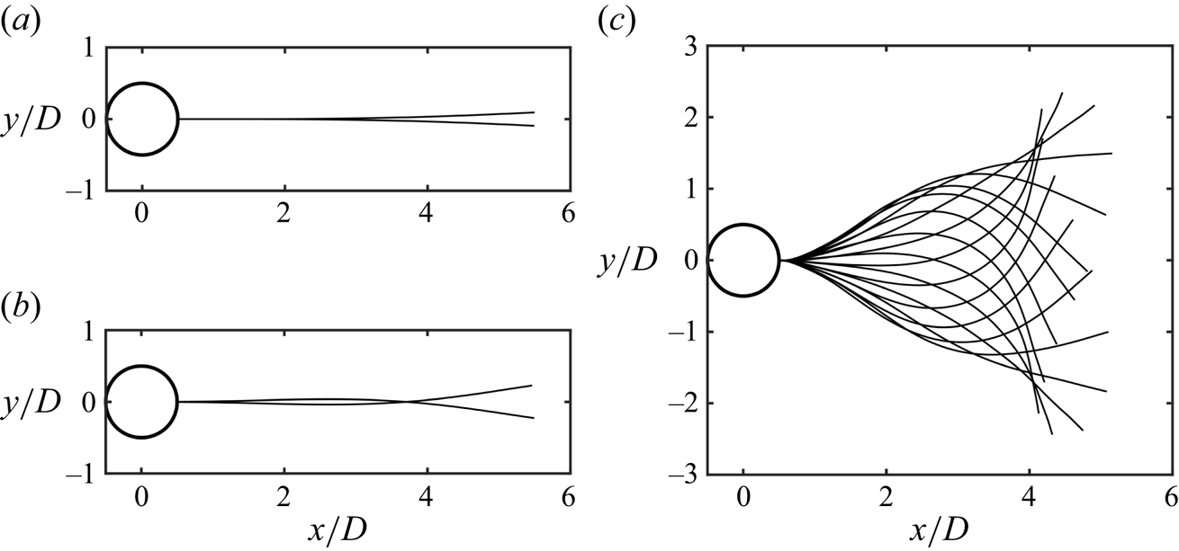
As the flexible film interacts with the cylinder wake, we identify four distinct kinematic regimes, which successively emerge with the increase of the film streamwise length, viz., (i) keeping stationary, (ii) deflection flutter, (iii) hybrid flutter and (iv) travelling-wave flapping (figure 2a). Given that the experiments conducted with the 0.1-mm-thick flexible film involve most of the representative coupling states, the results introduced herein will mainly be predicated on the observations and analyses of this specific film unless explicitly stated. Remarkably, the film flutters in regimes (ii) and (iii) appear disordered and aperiodic unexpectedly, which are new phenomena significantly different from the results in previous studies (see supplementary movies S1 and S2, available at https://doi.org/10.1017/jfm.2024.327). In the previous numerical simulations, the film in the cylinder wake always fluttered or flapped periodically irrespective of the streamwise length (Lee & You Reference Lee and You2013; Wu et al. Reference Wu, Qiu, Shu and Zhao2014; Sahu et al. Reference Sahu, Furquan and Mittal2019; Pfister & Marquet Reference Pfister and Marquet2020; Furquan & Mittal Reference Furquan and Mittal2021). Additionally, in the experiment of Shukla et al. (Reference Shukla, Govardhan and Arakeri2013), the aperiodic flutter of the flexible film in the cylinder wake only occurred when the flexible film was long enough to yield a very small effective bending stiffness (see (1.1a,b)), as an example,  $L/D=5$ and
 $K_B\sim O(10^{-4})$, three orders of magnitude lower than the minimum
 $K_B=1.82\times 10^{-1}$ where the aperiodic flutter emerges in our experiment. Moreover, an isolated flexible film with its leading edge pinned in the uniform flow also exhibits aperiodic undulation, which, however, is merely reported in the case of a long film with a very small
 $K_B$ as well, for example,
 $K_B\sim O(10^{-3})$ in Alben & Shelley (Reference Alben and Shelley2008) and
 $K_B\sim O(10^{-4})$ in Chen et al. (Reference Chen, Jia, Wu, Yin and Ma2014). Given the aperiodic flutters in the present research, we define the amplitude of the film statistically as
 $\tilde {A}=2\sqrt {2} y_{{rms}}^{s/L=1}$, where
 $y^{s/L=1}$ denotes the vertical displacement (in the
 $y$ direction) of the film's trailing edge (refer to figure 1). Thereupon, when the motion of the film is periodic, the statistical amplitude
 $\tilde {A}$ is equivalent to the peak-to-peak amplitude; in contrast, if the motion of the film is aperiodic, the statistical amplitude is an equal-energy characterization of the time-varying amplitude in essence.
Motion states of the 0.1 mm thick film in the cylinder wake. (a) Trailing-edge amplitudes  $\tilde {A}/D$ (left-hand vertical axis and triangular markers), self-similarity coefficients
 $\gamma ^\ast$ (right-hand vertical axis and square markers) and largest Lyapunov exponents
 $\lambda _1$ (top coordinate and circled plus markers) as functions of the non-dimensional film length
 $L/D$. For each regime separated by light-coloured blocks, sequences of instantaneous deformations are incorporated to show the representative motion patterns. (b) Phase trajectories of (i) trailing-edge point for
 $L/D = 1.0$, (ii) trailing-edge point for
 $L/D = 3.0$, (iii) trailing-edge point (
 $s/D=5$) and
 $s/D=3$ point for
 $L/D = 5.0$. Here, the vertical velocity
 $U_y{/U}_\infty$ and the displacement
 $y/D$ of the point are fivefold refined by modified Akima piecewise cubic interpolation to enhance the fineness of data and the accuracy of the phase trajectories (Akima Reference Akima1970; Moler Reference Moler2019). (c) Short-time fluctuations of the film motion in the
 $y$ direction with unit-amplitude rescaling
 $[y_{rms}]_t^\ast =[y_{{rms}}]_t/[y_{rms}]_t^{s=L}$ vary with time within 10 s, by which the self-similarity is revealed: (i)
 $L/D = 1.0$; (ii)
 $L/D = 3.0$; (iii)
 $L/D = 5.0$. (d) Cross-correlation coefficients,
 $c_r(t)={Corr}( \overline {[y_{rms}]_{t}^\ast },[y_{rms}]_t^\ast )$, as a function of time
 $t$ within 10 s: (i)
 $L/D = 1.0$; (ii)
 $L/D = 3.0$; (iii)
 $L/D = 5.0$. .

In the stationary regime (i) ( $L/D \lesssim 0.5$, the red region in figure 2a), the flexible film behaves like a rigid plate in the cylinder wake without any vibration or deflection, and obviously, its amplitude is
 $\tilde {A}/D = 0$. Nevertheless, in our previous study on the flexible film behind a circular cylinder, the film with a length of
 $L/D = 0.5$ showed small-amplitude flutter as we adopted a softer film material and higher free stream velocities (
 $U_\infty > 20\ \text {m s}^{-1}$) (Duan & Wang Reference Duan and Wang2021). This discrepancy lies on the competition between the stabilization of the bending force inside the film and the destabilization of the fluid force. We will expatiate on the instability mechanism of the short flexible film through the stability theory in § 3.2.
In the regime of deflection flutter (ii) ( $L/D = 1\sim 2$, the yellow region in figure 2a), the film commences to interact with the vortices shed from the cylinder, and flutter aperiodically with a very small amplitude
 $\tilde {A}/D \sim O(10^{-2})$ (figure 2bi and supplementary movie S1). This small-amplitude flutter bears a striking resemblance to the deflection of a cantilever beam described by the first-order Euler–Bernoulli mode. At this stage, the deformation envelope contains only one node located at the junction between the cylinder rear and the leading edge of the film. All the points on the film flutter with the same phase, and they deflect towards a single direction at a certain time. The maximum deflection angle is less than
 $7^\circ$. Hence, we characterize the aperiodic small-amplitude motion of the film in this regime as deflection flutter.
In the regime of hybrid flutter (iii) ( $L/D = 2.5\sim 4$, the blue region in figure 2a), the film still keeps a pretty small-amplitude flutter,
 $\tilde {A}/D \sim O(10^{-1})$, despite its amplitude surpassing that in regime (ii) by an order. The flutter also appears aperiodic and disordered (figure 2bii), but exhibits two distinct modes alternately, as in supplementary movie S2. One mode is similar to the deflection flutter in regime (ii), i.e. all the points on the film move in phase, whereas the other mode behaves as a cambered-flection flutter, whose feature in substance accords with the second Euler–Bernoulli mode that portrays the flection of a cantilever beam. In the flection mode, there are two wave nodes on the envelope of the deformation sequence (figure 2a); besides, different points on the film show a perceptible phase difference. We observed in the experiment that the two modes alternate randomly and spontaneously with an alternating time scale of the order of
 $O(10^{-1})$ s.
For the disordered aperiodic flutters of the film in regimes (ii) and (iii), we calculate the largest Lyapunov exponent  $\lambda _1$ of the vertical displacement of the trailing edge, in order to quantify this disordered dynamics (refer to the phase trajectories for
 $L/D = 1$ and
 $L/D=3$ in figure 2b) (Abarbanel et al. Reference Abarbanel, Brown, Sidorowich and Tsimring1993; Connell & Yue Reference Connell and Yue2007; Goza, Colonius & Sader Reference Goza, Colonius and Sader2018). The largest Lyapunov exponent
 $\lambda _1$ describes the divergence and convergence of the nearby initial orbits in the phase space of a dynamical system; for uniformly discrete data, it is defined as
 \begin{equation} \lambda_1=\frac{1}{N_T}\sum_{k=1}^{M}\log_2{\frac{{d}^\prime (t_k)}{{d}(t_{k-1})}},\end{equation}
where  $N_T$ is the total number of the evaluated data series,
 $M$ the number of iterations,
 $d$ the Euclidean distance between two nearest points on adjacent phase trajectories in phase space and
 $d^\prime$ the distance between the two points after evolution within a time step of
 $t_k-t_{k-1}$ (Wolf et al. Reference Wolf, Swift, Swinney and Vastano1985; Abarbanel et al. Reference Abarbanel, Brown, Sidorowich and Tsimring1993; Pikovsky & Politi Reference Pikovsky and Politi2016). Here, a logarithm with base 2 is applied to define
 $\lambda _1$ so that
 $\lambda _1$ has the units of a ‘bit’ in information theory. A positive
 $\lambda _1$,
 $\lambda _1>0$, corresponds to an exponential divergence of the orbits, indicating the system becomes unpredictable rapidly, namely, a chaotic system, whereas a negative
 $\lambda _1$,
 $\lambda _1<0$, a convergence of the system, and it is then evident that
 $\lambda _1\rightarrow 0$ signifies a stable periodic system (Pikovsky & Politi Reference Pikovsky and Politi2016). To determine the largest Lyapunov exponent
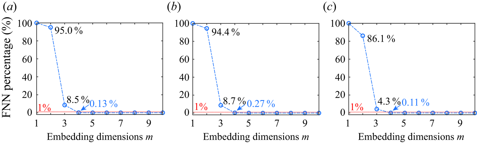
 $\lambda _1$ for each case, we embed the vertical motion of the trailing edge into a four-dimensional phase space using the time delay algorithm to reconstruct an attractor without ambiguity (Abarbanel et al. Reference Abarbanel, Brown, Sidorowich and Tsimring1993; Cellucci, Albano & Rapp Reference Cellucci, Albano and Rapp2003; Majumdar, Bose & Sarkar Reference Majumdar, Bose and Sarkar2022). The largest Lyapunov exponent
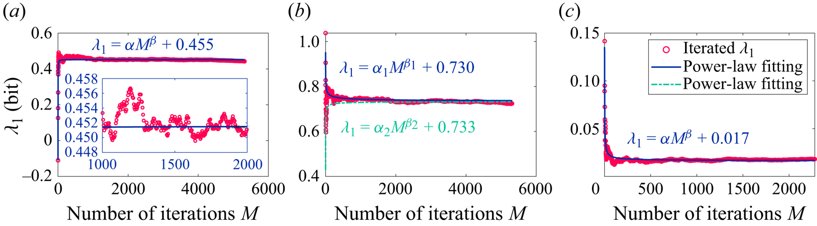
 $\lambda _1$ for each case is iterated out with Wolf's algorithm on the reconstructed four-dimensional attractor (Wolf et al. Reference Wolf, Swift, Swinney and Vastano1985) (see Appendix A), and the results of
 $\lambda _1$ are incorporated in figure 2(a). Here, in the phase-space reconstruction, we follow the broadly used assumption in the embedding theorem that the time delay and the embedding dimension are two uncorrelated parameters (Kennel, Brown & Abarbanel Reference Kennel, Brown and Abarbanel1992; Kantz & Schreiber Reference Kantz and Schreiber2003). Then, as presented in Appendix A, the optimal value of time delay for phase-space reconstruction is determined with the average mutual information (AMI) algorithm (Fraser & Swinney Reference Fraser and Swinney1986; Cellucci et al. Reference Cellucci, Albano and Rapp2003), and the embedding dimension is obtained by reconciling the false nearest neighbours (FNN) algorithm (Kennel et al. Reference Kennel, Brown and Abarbanel1992; Wallot & Mønster Reference Wallot and Mønster2018) and the requirement of Wolf's Lyapunov exponent algorithm (Wolf et al. Reference Wolf, Swift, Swinney and Vastano1985). It is worth noting that Wolf's algorithm has been adopted to the analyses of flow–structure interactions by Connell & Yue (Reference Connell and Yue2007) and Goza et al. (Reference Goza, Colonius and Sader2018); however, they did not give rigorous details on the computations. An accurate estimation of the largest Lyapunov exponent relies on the appropriate phase space reconstruction and the proper prescription of iteration parameters, which depend on the nature of data (Cellucci et al. Reference Cellucci, Albano and Rapp2003; Kantz & Schreiber Reference Kantz and Schreiber2003). Therefore, a simple use of Wolf's algorithm would not yield an ideal outcome; in this situation, the applications of this algorithm by different researchers to address the same or similar problems may acquire Lyapunov exponents that exhibit substantial deviations. Here, in pursuit of utmost accuracy and reproducibility in estimating
 $\lambda _1$ for flow–structure interactions, we present a solving framework for the largest Lyapunov exponent in fastidious detail, which integrates Wolf's algorithm with a series of parameter-optimization processings. It is anticipated that this framework would yield an optimal estimation for
 $\lambda _1$. For coherence of the main text, we put the details of the solving procedure for the Lyapunov exponent in Appendix A.
As illustrated in figure 2(a), the largest Lyapunov exponents are always positive for the cases of  $L/D = 1\sim 4$ (
 $\lambda _1 > 0.4$ bit), where the maximum attains
 $\lambda _1\approx 0.8$ bit at
 $L/D=2$. This result accords with our observations of the disordered and aperiodic flutters in regimes (ii) and (iii) (figures 2a and 2b; supplementary movies S1 and S2), which further corroborates the fact that the flutters tend to chaos. From the viewpoint of information theory, the positive Lyapunov exponent measures how rapidly the system creates information (Wolf et al. Reference Wolf, Swift, Swinney and Vastano1985). Use
 $L/D=3$ as an example, whose amplitude is approximately
 $0.224D$. Considering the measurement accuracy of the deformation in our experiment attains the subpixel magnitude of approximately
 $O(10^{-2})$ mm (§ 2), we, therefore, have an initial inherent uncertainty of approximately 1/500, equivalent to data with a 9-bit acquisition. The largest Lyapunov exponent for
 $L/D=3$ is
 $\lambda _1\approx 0.75$ bit, indicating we will lose the predictability of this case after 12 samples ((9 bits)/(0.75 bits)) on average since 9 bits of new information is produced after this time (Pikovsky & Politi Reference Pikovsky and Politi2016). The sampling frequency of our experiment is 800 Hz (1/800 s per sample); hence, the motion of the film with
 $L/D=3$ only has a predictability time of 0.015 s. In contrast to the film flutters, the flow fields in regime (ii) and (iii) show perceptible periodicity (refer to § 3.3), which implies a non-complete coupling state between the film and the flow field, in other words, the film and the periodic vortices do not lock in with each other. Synthesizing the previous research, we notice this non-complete coupling state resembles the ‘entraining state’ of a fish (e.g. rainbow trout and smallmouth bass) behind an obstacle in the flow, where the fish's body is relatively straight and presents an irregular small-amplitude flutter without rhythmic body undulation (Webb Reference Webb1998; Liao Reference Liao2007; Przybilla et al. Reference Przybilla, Kunze, Rudert, Bleckmann and Brücker2010; Taguchi & Liao Reference Taguchi and Liao2011). It naturally occurs to us that we might be able to utilize the largest Lyapunov exponent to quantitively fathom out how irregular the flutter of the fish is under the entraining state. It will be not only interesting but valuable to find out the relationships between
 $\lambda _1$ and the fish species, the free stream velocities, and so forth, which would help to construct a biomechanical model for the entraining state.
In the regime of travelling-wave flapping (iv) ( $L/D\gtrsim 5$, the green region in figure 2a), the film jumps to stable periodic flapping, which is completely locked-in with the flow field (refer to supplementary movies S3 and S4, and figure 2biii). The amplitude of the film soars to the magnitude of
 $\tilde {A}/D \sim O(1)$, accompanied by a significant increase of the deformation curvature. This periodic flapping can be regarded as a bending wave traveling along the film, and then can be depicted by a wavefunction (see § 3.4); as a result, we designate it as a travelling-wave flapping. Taking the flapping at
 $L/D = 5$ as an example, we find the amplitude reaches
 $\tilde {A}/D = 5.1$ (figure 2a), while the flapping frequency is identical to that of the flow field, 30.8 Hz for both of them. The corresponding largest Lyapunov exponent approaches zero,
 $\lambda _1 \sim O(10^{-2})$ (figure 2a), demonstrating that the film flapping follows a stable limit cycle in the phase space (see figure 2biii), as well as an almost constant amplitude and frequency. The exponent
 $\lambda _1$ tending to zero also implies that the periodic flapping is highly self-sustained, which can quickly revert to the limit cycle after being perturbed. By comparison, in the experimental research of Zhang et al. (Reference Zhang, Childress, Libchaber and Shelley2000), where the flapping of an isolated flexible filament in the soap film is examined, the flapping filament can be easily switched to the stretched-straight state by externally forcing the filament. Thus, we presume the flapping of the film in the cylinder wake is more robust, which is attributed to the robustness of the vortex shedding.
The largest Lyapunov exponent aids us in quantitatively delineating and differentiating the periodic (regime iv) and chaotic (regimes ii and iii) motions of the flexible film; nevertheless, we have the question of how to further discriminate the two chaotic flutters in regimes (ii) and (iii) quantitatively. Here, we further propose the short-time self-similarity coefficient  $\gamma$ to characterize the motion state changing with the film length
 $L/D$. The deflection flutter in regime (ii) appears a steady ‘stochastic process’ (figure 2bi and supplementary movie S1). In contrast, the flutter in regime (iii) is a hybrid of deflection and flection; as the flutter switches from the deflection to the flection, the associated statistics will change forthwith, meaning the flutter in regime (iii) is similar to a non-steady ‘stochastic process’ (figure 2bii and supplementary movie S2). It should be accentuated that within the framework of classical mechanics, the disordered aperiodic flutter of the film does not possess a truly random nature. Instead, its fundamental essence resides in being a deterministic chaotic system that remains extremely sensitive to initial conditions or small perturbations (Abarbanel et al. Reference Abarbanel, Brown, Sidorowich and Tsimring1993; Kantz & Schreiber Reference Kantz and Schreiber2003). We employ the terminology of a ‘stochastic process’ merely for the qualitative depiction of the film's motion characteristics. The above analysis tells us that the flutters in regime (ii) over different time intervals possess self-similarity, whereas in regime (iii), this self-similarity disappears. Besides, the stable periodic flapping in regime (iv) is also believed to be controlled by self-similarity. Since it is observed in the experiment that the alternating time scale between deflection and flection in regime (iii) is around
 $O(10^{-1})$ s (see supplementary movie S2), we take
 $\Delta t= 0.125$ s as the length of the time interval to assess the short-time statistics. At each moment
 $t$, we can obtain a short-time fluctuation
 $[y_{rms}]_t$ of the vertical displacement of the whole film in a time interval
 $[t-\Delta t/2, t+\Delta t/2]$, which is then normalized by the value of the trailing edge
 $[y_{rms}^{s=L}]_t$, namely,
 $[y_{rms}]_t^\ast =[y_{rms}]_t/[y_{rms}^{s=L}]_t$. Obviously,
 $[y_{rms}]_t^\ast$ characterizes the short-time statistical quality of the film motion in the time interval
 $[t-\Delta t/2, t+\Delta t/2]$; we emphasize here that
 $[y_{rms}]_t^\ast$ is a function of time
 $t$ and curvilinear Lagrangian coordinate
 $s$. Figure 2(ci–iii) show the variations of
 $[y_{rms}]_t^\ast$ with time
 $t$ for
 $L/D = 1.0$,
 $L/D = 3.0$ and
 $L/D = 5.0$, respectively. One can see for
 $L/D = 1.0$ (figure 2ci) and
 $L/D = 5.0$ (figure 2ciii), the short-time fluctuations
 $[y_{rms}]_t^\ast$ accord well with each other at different moments, manifesting a strong self-similarity, in addition to which the case of
 $L/D = 5.0$ shows a better self-similarity due to its regular periodicity. However, the tendencies of
 $[y_{rms}]_t^\ast$ for
 $L/D = 3.0$ vary with time conspicuously (figure 2cii), corresponding to the alternations of the deflection flutter and the flection flutter. We use Pearson's correlation coefficient to measure the linear similarity among
 $[y_{rms}]_t^\ast$ at different times. As such, the correlation coefficient is calculated by
 $c_r(t)={Corr}( \overline {[y_{rms}]_t^\ast },[y_{rms}]_t^\ast )$ with the time-averaged value,
 $\overline {[y_{rms}]_t^\ast }$, as the benchmark. For the cases of
 $L/D = 1.0$ and
 $L/D = 5.0$ with high self-similarity, the temporal variations of the correlation coefficient
 $c_r(t)$ remain nearby flat and close to unity (figure 2ci,iii), whereas
 $c_r(t)$ for the case of hybrid flutter of
 $L/D = 3.0$ experiences definite fluctuations (figure 2cii). Consequently, the self-similarity coefficient
 $\gamma$ is defined by the root-mean-square (r.m.s.) value of
 $c_r(t)$, i.e.
 $\gamma ={\rm r.m.s.}[c_r(t)]$, and for comparative purposes,
 $\gamma$ is then rescaled by the value of the case of
 $L/D = 1.0$ as
 $\gamma ^\ast =\gamma /\gamma ^{L/D=1.0}$. A small value of
 $\gamma ^\ast$ means a high self-similarity while a large value a low self-similarity.
In figure 2(a), we compare  $\gamma ^\ast$ for each case tested. It is illustrated that
 $\gamma ^\ast$ exhibits changes in order of magnitude with the transition of regimes,
 $\gamma ^\ast \equiv 0$ in stationary regime (i),
 $\gamma ^\ast \sim O(10^0)$ for the small-amplitude deflection flutter in regime (ii),
 $\gamma ^\ast \sim O(10^1)$ for the hybrid flutter in regime (iii) and
 $\gamma ^\ast \sim O(10^{-1})$ for the travelling wave flapping in regime (iv). The self-similarity coefficient
 $\gamma ^\ast$, therefore, quantifies the transitions of the motion states with length; in particular, the two small-amplitude chaotic flutters in regimes (ii) and (iii) are distinguished clearly. Compared with the superficial parameter (the trailing-edge amplitude
 $\tilde {A}$), the value of
 $\gamma ^\ast$ extracts the inherent kinematic characteristics of different motion regimes. This method that quantifies the kinematic characteristics with self-similarity coefficient
 $\gamma ^\ast$ may also be generalized to analyse the motion of a flexible film in any configurations so as to verify whether and when the motion incorporates multiple modes, for example, the chaotic flapping of an isolated flexible flag in the study of Connell & Yue (Reference Connell and Yue2007); in addition, it is not limited to two-dimensional cases (Huang & Sung Reference Huang and Sung2010).
3.2. Instability and flow fields for the short film
For the motion of the flexible film in the cylinder wake, another issue of our main interest is to explore the instability mechanism. In our previous experiment (Duan & Wang Reference Duan and Wang2021), the film with  $L/D=0.5$ showed visible flutter in the cylinder wake, yet it remains stationary in the current experiment. When the length of the film is large enough, it is evident that the flapping or fluttering is attributed to the direct and strong interactions with the large-scale vortices from the cylinder, which is visually demonstrated by the evolution of flow structures presented in § 3.3 for
 $L/D=3.0$ and
 $4.0$, and in § 3.5 for
 $L/D=5.0$. Nevertheless, what is the kinetic mechanism that dictates the flutter of a short film (for example,
 $L/D=0.5$)? The short film is entirely encompassed by the recirculation region of the cylinder wake, where the flow is relatively steady in comparison with the region after vortex shedding (Duan & Wang Reference Duan and Wang2021). Hence, we attempt to solve the stability boundary of the short film via the linear stability analysis, thereby providing guidance for us to explore the physical mechanism that excites the flutter. The slight flutter of a clamped film can be deemed as the bending of a cantilever beam under the small load of the ambient flow field, and is thus governed by the Euler–Bernoulli theory (Argentina & Mahadevan Reference Argentina and Mahadevan2005; Connell & Yue Reference Connell and Yue2007; Alben & Shelley Reference Alben and Shelley2008; Shoele & Mittal Reference Shoele and Mittal2016). Considering the two-dimensional condition (the spanwise height is unit length,
 $b = 1$), a film with a linear density
 $\rho _sh$ and a bending stiffness
 $B$ flutters with a small vertical displacement
 $\eta (x,t)$ in the flow with a fluid density
 $\rho _f$, which satisfies the kinetic equation
 \begin{equation} \rho_sh\frac{\partial^2\eta}{\partial t^2}- \frac{\partial}{\partial x}\left(\tau(x)\frac{\partial\eta}{\partial x}\right)+ B\frac{\partial^4\eta}{\partial x^4}= \varUpsilon(x,t),\end{equation}
where  $x$ is the streamwise Cartesian coordinate (figure 1a),
 $\tau (x)$ originating from the friction acting on the film along the tangential direction, which manifests itself in the tensile stress (
 $\tau > 0$) or the compressive stress (
 $\tau < 0$) inside the film;
 $\varUpsilon (x,t)$ the vertical force (lift) on the film per unit length by the fluid in the vicinity, which is equal in magnitude but opposite in sign to the force acting on the fluid by the film. According to Newton's law, the force acted by the film on the fluid per unit length is equivalent to the change rate of the momentum of the ambient fluid induced by the displacement
 $\eta (x,t)$ of the film (Coene Reference Coene1992; Connell & Yue Reference Connell and Yue2007; Michelin & Doaré Reference Michelin and Doaré2013), that is,
 \begin{equation} \varUpsilon(x,t)={-}\frac{\mathrm{D}}{\mathrm{D} t}\left(m_a\frac{\mathrm{D}}{\mathrm{D} t}\eta\right);\end{equation}
here,  $m_a$ is the added mass per unit length, and material derivative
 $\mathrm {D}/\mathrm {D} t=\partial /\partial t+U(\partial /\partial x)$. Note that
 $U$ in the material derivative is the velocity of the flow over the film, which is equal to the free stream velocity
 $U_\infty$ for an isolated film in the flow field. However, for the short film surrounded by the recirculating flow, the velocity of the flow over the film
 $U$ is less than the free stream velocity
 $U_\infty$ and in the opposite direction to the free stream (
 $U$ towards the
 $-x$ direction). As a result, the tangential force
 $\tau$ exerted by the fluid on the film yields a compressive effect on the film, acting as compressive stress. In search of a theoretical solution for the nonlinear differential equations (3.2) and (3.3), we consider implementing linearization to them with the three assumptions: (i) the velocity of the flow over the film,
 $U$, is linearly proportional to the free stream velocity
 $U_\infty$, namely
 $U=\epsilon U_\infty$; (ii) the internal tangential stress
 $\tau$ is a constant value
 $\tau _0$ (Argentina & Mahadevan Reference Argentina and Mahadevan2005; Connell & Yue Reference Connell and Yue2007); (iii) the added mass
 $m_a$ remains constant (Coene Reference Coene1992). Introducing the three linearization assumptions to (3.2) and (3.3), and then non-dimensionalizing the equations with
 $U_\infty$,
 $L$ and
 $\rho _f$, we obtain a fourth-order linear differential equation for
 $\eta (x,t)$,
 \begin{equation} (S+m_a^\ast)\frac{\partial^2 \eta}{\partial t^2}+ (\epsilon^2m_a^\ast - \tau_0^\ast) \frac{\partial^2\eta}{\partial x^2}+K_B\frac{\partial^4\ \eta}{\partial x^4} +2\epsilon m_a^\ast\frac{\partial^2\eta}{\partial x\partial t}=0,\end{equation}
where dimensionless parameters  $m_a^\ast =m_a/(\rho _f L)$,
 $\tau _0^\ast =\tau _0/(\rho _f U_\infty ^2 L)$; the mass ratio
 $S$ and the effective bending stiffness
 $K_B$ are defined in (1.1a,b). The three terms,
 \begin{equation} m_a^\ast\frac{\partial^2\ \eta}{\partial t^2},\quad \epsilon^2m_a^\ast\frac{\partial^2\eta}{\partial x^2}\quad \mathrm{and} \quad 2\epsilon m_a^\ast\frac{\partial^2\eta}{\partial x\partial t}, \end{equation}
associated with the added mass  $m_a^\ast$ in (3.4) refer to translation inertial force, centrifugal force and Coriolis force, respectively (Triantafyllou Reference Triantafyllou1992); particularly, the term of centrifugal force,
 $\epsilon ^2 m_a^\ast (\partial ^2\eta / \partial x^2)$, represents the destabilization of the K–H instability on the interfaces. Considering a perturbation with frequency
 $\omega$ and wavenumber
 $k$ in the form
 $\eta (x,t)=\eta _0e^{{\rm i}(kx-\omega t)}$, we obtain a quadratic function for
 $\omega$,
 \begin{equation} -\!(S+m_a^\ast)\omega^2+2\epsilon m_a^\ast k\omega- (\epsilon^2 m_a^\ast -\tau_0^\ast)k^2+K_B k^4=0.\end{equation}
Note that both the frequency  $\omega$ and the wavenumber
 $k$ in (3.6) are dimensionless parameters. The former is obtained by normalizing the dimensional frequency with
 $L$ and
 $U_\infty$, while the latter by normalizing the dimensional wavenumber with
 $L$. Solving (3.6), we acquire the dispersion relation linking the frequency
 $\omega$ and the wavenumber
 $k$, namely
 $$\begin{gather} \omega =\frac{k}{S+m_a^\ast}(\epsilon m_a^\ast{\pm} \sqrt{\varDelta_k}), \end{gather}$$
 $$\begin{gather}\varDelta_k ={-}\epsilon^2 m_a^\ast S+(S+m_a^\ast)(K_B k^2+\tau_0^\ast). \end{gather}$$
For  $\varDelta _k \geq 0$ in (3.7b), the system remains neutrally stable, while for
 $\varDelta _k<0$,
 $\omega$ contains imaginary part
 $\mathrm {i} \omega _\mathrm {i}$, meaning the perturbation will undergo an exponential growth with time
 $t$, and consequently the system becomes unstable. Here, we give a simple discussion regarding the physical implications of
 $\varDelta _k$. The first term in
 $\varDelta _k$,
 $-\epsilon ^2 m_a^\ast S$, is negative, representing the destabilizing effect of the ever-present K–H instability. In the second term of
 $\varDelta _k$, the constantly positive component
 $K_B k^2$ describes the stabilizing effect of the elasticity of the film; a positive
 $\tau _0^\ast$ (
 $\tau _0^\ast >0$) means the tensile stress stabilizes the film whereas a negative
 $\tau _0^\ast$ (
 $\tau _0^\ast <0$) means the compressive stress destabilizes the film. For the film with
 $L/D = 0.5$ encompassed in the recirculation region, if its bending stiffness is large enough, it keeps stable even though the friction from the reverse flow in the recirculation region generates compressive stress, namely, regime (i) in § 3.1. Note that (3.7a,b) is not limited to the film in the recirculation region of the cylinder, but also holds for the isolated film in uniform flow, where the coefficient
 $\epsilon =1$ for the leading-edge pinned film (normal configuration) and
 $\epsilon =-1$ for the trailing edge pinned film (inverted configuration). Thus, we can interpret and compare some phenomena in the literature with (3.7a,b). For the isolated film with the normal configuration, the friction from the ambient flow stretches and stabilizes the film; on the contrary, for the inverted configuration, the friction acts as compressive stress and destabilizes the film. Thus, the film with the inverted configuration is more prone to instability than the normal configuration. Besides, for the short film surrounded by the recirculation region of the cylinder or the inverted film, an interesting inference from (3.7a,b) is that owing to the destabilizing effect of the compressive stress, the film with its mass tending to zero (
 $S\rightarrow 0$) can still become unstable, provided that the condition
 $|\tau _0^\ast |>K_B k^2$ is satisfied. This theoretical inference confirms the hypothesis of Kim et al. (Reference Kim, Cossé, Huertas Cerdeira and Gharib2013) from experiments that the mass ratio is not the prerequisite for the instability mechanism of the inverted film. Conversely, for a massless film with the normal configuration, the instability cannot be accomplished (Connell & Yue Reference Connell and Yue2007).
According to (3.7b), we can determine the stability boundary by applying  $\varDelta _k = 0$, which gives
 \begin{equation} K_B=k^{{-}2} \left( \frac{\epsilon^2 m_a^\ast S}{S+m_a^\ast} -\tau_0^\ast \right).\end{equation}
The dimensionless added mass  $m_a^\ast$ is a function of the wavenumber
 $k$ in the form of
 $m_a^\ast =2/k$ by solving the Laplace equation of potential flow and the linearized Bernoulli equation (Coene Reference Coene1992; Connell & Yue Reference Connell and Yue2007). In addition, in the previous studies (Shelley, Vandenberghe & Zhang Reference Shelley, Vandenberghe and Zhang2005; Jia et al. Reference Jia, Li, Yin and Yin2007; Eloy et al. Reference Eloy, Lagrange, Souilliez and Schouveiler2008, Reference Eloy, Kofman and Schouveiler2012), the discussions for the instability of a film were contextualized in the parameter space spanned by the reduced velocity
 $U^\ast$ and the mass ratio
 $S$, where the reduced velocity is
 $U^\ast =\sqrt {1/K_B}$. Substituting the above two terms for the parameters
 $m_a^\ast$ and
 $K_B$ in (3.8), respectively, we finally derive the stability boundary as
 \begin{equation} U^\ast = k\sqrt{\frac{2+kS}{2\epsilon^2 S-\tau_0^\ast (2+kS)}}.\end{equation}
In our experiment, the flow velocity in the recirculation region attains approximately 1/4 of the free stream velocity, which agrees with the results in the literature (Beaudan Reference Beaudan1995; Parnaudeau et al. Reference Parnaudeau, Carlier, Heitz and Lamballais2008), so we take  $\epsilon =-1/4$ as the linearization coefficient for the oncoming velocity
 $U$. Given that the short film exbibits instability in the first-order mode (see subpanels in figure 3a), the corresponding wavenumber of a cantilever beam, i.e.
 $k=1.875$, is introduced in (3.9) (Jia Reference Jia2014). The compressive stress
 $\tau _0^\ast$ arises out of the friction exerted on the film by the reverse flow in the recirculation region, but unfortunately, there is no directly available data for the skin friction of the film surrounded by the recirculation region of a circular cylinder. For this reason, we endeavour to estimate a reasonable compressive stress
 $\tau _0^\ast$ with the skin friction coefficient given by Castro & Haque (Reference Castro and Haque1987), where the friction coefficient on a plate in the recirculation region of a bluff body was measured with the pulsed-wire skin-friction probe. The Reynolds number based on the scale of the bluff body is
 $Re_D=1.49\times 10^4$ in Castro & Haque (Reference Castro and Haque1987), close to the Reynolds number
 $Re_D=1.34\times 10^4$ in the present experiment. After integrating the friction along the streamwise length of the film, we secure an estimated stress value of
 $\tau _0^\ast \sim -2\times 10^{-3}$. We must acknowledge that the above estimation for
 $\tau _0^\ast$ is not rigorous; be that as it may, we believe the estimated value is at least acceptable in the order of magnitude. The stability boundary determined by
 $\tau _0^\ast \sim -2\times 10^{-3}$ is shown in figure 3(a) with the green solid line; besides, the boundary with vanishing
 $\tau _0^\ast$ is also plotted in figure 3(a) using the black dashed line for comparison. The region over the boundary represents an unstable coupling system, where the perturbation undergoes an exponential increase, and then the film loses stability. One can see that the introduction of a negative
 $\tau _0^\ast$, viz. compressive stress, diminishes the critical reduced velocity
 $U^\ast$. Moreover, the smaller the mass ratio
 $S$, the more significant the destabilizing effect of the compressive stress (
 $\tau _0^\ast <0$); particularly, as
 $S \lesssim 10^{-1}$, a considerable diminution of the
 $U^\ast$ appears, as shown by the shaded area with diagonals in figure 3(a). The mass ratio
 $S$ in the water is lower by a magnitude of
 $O(10^{-3})$ than that in air for a certain flexible film, so it is of particular importance to account for the influence of
 $\tau _0^\ast$ as the experiment is conducted in water flow.
Results of linear stability analysis. (a) Stability boundaries of the film motion in the  $S$–
 $U^\ast$ plane solved by (3.2)–(3.9), above which the perturbations undergo such an exponential growth that the film loses it stability. The green solid line shows the stability boundary with the linearized tangential stress
 $\tau _0^\ast$ considered, while the black dashed line is without the stress
 $\tau _0^\ast$. The diagonal shading between the two boundaries gives the diminution of the reduced velocity due to the tangential stress
 $\tau _0^\ast$. Here,
 $\tau _0^\ast \sim -2\times 10^{-3}$. Sequences of instantaneous deformations for the film of
 $L/D=0.5$ after instability are also incorporated in this panel. (b,c) (i) Finite time Lyapunov exponent (FTLE) fields calculated from the phase-averaged velocity fields (see Appendix B) (He et al. Reference He, Pan, Feng, Gao and Wang2016; Wang & Wang Reference Wang and Wang2021a), and (ii) time-averaged vorticity fields superimposed with the time-averaged streamlines; (b) for
 $L/D=0.5$ and (c) for
 $L/D=1.0$.

In the  $S-U^*$ parameter plane of figure 3(a), we plot the state point
 $(S, U^*)$ for the
 $L/D=0.5$ film with a thickness of 0.1 mm in the present study (
 $U_\infty =10\ \text {m s}^{-1}$) together with the state points
 $(S, U^*)$ for the
 $L/D = 0.5$ film at
 $U_\infty =20\ \text {m s}^{-1}$ and
 $30\ \text {m s}^{-1}$ in our previous experiment (Duan & Wang Reference Duan and Wang2021). The
 $L/D=0.5$ film in the present study remains stationary, along with which its
 $(S, U^\ast )$ point is located in the stable region of the
 $S$–
 $U^\ast$ plane. By comparison, in the experiment of Duan & Wang (Reference Duan and Wang2021), the film just destabilizes to a very small flutter at
 $U_\infty = 20\ \text {m s}^{-1}$, and its
 $(S, U^\ast )$ exactly falls near the theoretical stability boundary (a critical state); with the velocity raised to
 $U_\infty = 30\ \text {m s}^{-1}$, the film flutters noticeably, and unsurprisingly its
 $(S, U^\ast )$ point drops into the unstable region of the
 $S-U^\ast$ plane, as shown in figure 3(a). Consequently, for the short film of
 $L/D = 0.5$, our theoretical model accords well with the experimental data. However, it deviates from the experimental results as the length
 $L/D \gtrsim 1.0$. Notwithstanding the films of
 $L/D\gtrsim 1.0$ exhibiting an obvious flutter in the experiment (figure 2a), the corresponding state points still scatter in the stable region of the theoretical model (figure 3a). We, therefore, consider inquiring into the related reason from the flow fields. With the backward-time integration of the phase-averaged velocity fields for the cases of
 $L/D= 0.5$ and 1.0, we obtain their finite time Lyapunov exponent (FTLE) fields (Pan, Wang & Zhang Reference Pan, Wang and Zhang2009; He et al. Reference He, Pan, Feng, Gao and Wang2016; Wang & Wang Reference Wang and Wang2021a), as shown in figures 3(b) and 3(c). The convective material lines identified from the FTLE fields for the two cases reveal the formation and evolution of the periodic large-scale vortices that dominate the flow fields (see Appendix B for the detailed computation of the FTLE fields). For the case of
 $L/D = 1.0$, the separated shear layer from each side of the cylinder rolls up to form the large-scale vortex just at the trailing edge of the film, which results in a conspicuous interaction between the trailing edge and the material line of the vortex, as depicted in figure 3(c). From this perspective, the destabilization of the film is primarily induced by the large-scale vortex, whose perturbations are so strong that the case of
 $L/D = 1.0$ lies beyond the valid scope of the linear small-perturbation theory, thereby delivering an invalid linear stability analysis for this case. In comparison, concerning
 $L/D = 0.5$, the film entirely immerses in the recirculation region of the cylinder, and the large-scale vortex is formed downstream of the film's trailing edge without a direct influence on the film (figure 3b); under this situation, the flow condition in the vicinity of the film is broadly in line with the premises of the theoretical model. Hence, a substantial agreement between the stability analysis and the experiment results is drawn for
 $L/D = 0.5$. Briefly, the destabilization of a short film in the recirculation region of a circular cylinder stems from the combined destabilizing effects of the two factors: one is the K–H instability on the interface while the other is the negative tangential compressive stress (
 $\tau _0^\ast <0$) from the recirculating flow. Additionally, these two factors also hold for the destabilization of an inverted film in free stream. If the film is long enough, for example,
 $L/D\gtrsim 1.0$, the direct interaction between the film and the large-scale vortices from the cylinder will be the major responsibility for the flutter.
In order to further validate the theoretical analysis, we completed supplementary experiments for the film of  $L/D=0.5$, but different film materials and free stream velocities were employed (see table 1 in § 2). Specifically, PVC membranes with thicknesses of 0.045 mm and 0.022 mm were selected to fabricate the film of
 $L/D=0.5$. The density and Young's modulus of the PVC membrane were
 $1.28\times 10^3\ \mathrm {kg\ m}^{-3}$ and 1.12 GPa, respectively, which were measured in the same way as described in § 2. For the film with
 $h=0.045$ mm, the free stream velocities were
 $U_\infty =10\ \text {m s}^{-1}$ and
 $20\ \text {m s}^{-1}$, where the latter was very close to the critical instability velocity of the film observed in the experiment. For the film with
 $h=0.022$ mm, the free stream velocity of
 $U_\infty =10\ \text {m s}^{-1}$ was still selected in order to keep a consistent Reynolds number,
 $Re_D=1.33\times 10^4$, with other cases. The dimensionless parameter pair
 $(S, U^*)$ for the film with
 $h=0.022$ mm at
 $U_\infty =10\ \text {m s}^{-1}$ is (2.34, 11.00), while
 $(S, U^*)$ for the film with
 $h=0.045$ mm at
 $U_\infty =10\ \text {m s}^{-1}$ and
 $20\ \text {m s}^{-1}$ are (4.79, 3.76) and (4.79, 7.52), respectively. Notably, in the experiment, the free stream from the wind tunnel was carefully accelerated to the target velocity gradually, namely,
 $U_\infty =10\ \text {m s}^{-1}$ or
 $20\ \text {m s}^{-1}$, to avert the potential influence of hysteresis. At
 $U_\infty =10\ \text {m s}^{-1}$, the film with
 $h=0.022$ mm exhibits obvious flutter with the first-order mode, as shown by the sequence of instantaneous deformations integrated in figure 3(a) on the left-hand side, whereas the film with
 $h=0.045$ mm keeps stationary, which accord well with the scattering of the state points
 $(S, U^*)$ in the parameter plane for the two cases (figure 3a). As the velocity is increased to
 $U_\infty =20\ \text {m s}^{-1}$, the film with
 $h=0.045$ mm is also destabilized, as shown by the sequence of instantaneous deformations integrated in figure 3(a) on the right-hand side. The state point for this case drops near the stability boundary (figure 3a), approximately in agreement with the theoretical analysis. It is essential to point out that the present theoretical analysis is not impeccable, given that the influence of the vortex shedding is neglected. Although the film of
 $L/D =0.5$ is encompassed in the recirculation region and has no direct interactions with the large-scale vortices as mentioned above (figure 3b), the disturbance of the large-scale vortices can propagate forward, which is also the factor inducing the instability of the film. Nevertheless, the stability boundary according to the linear theory yields a tolerable consistency with the experimental data, implying this simple theory indeed catches the dominant factors. Two cases near the critical states, shown by blue cross maker ‘
 $\times$’ and blue diamond maker ‘
 $\Diamond$’, are located near but below the stability boundary in the
 $U^*$–
 $S$ plane, of which the relative
 $U^*$ errors are 4.9 % and 6.6 %, respectively. Consequently, the real stability boundary is bound to be lower than the present prediction, which indicates the influence of the vortex shedding outside the recirculation region.
Next, we discuss the influences of the short film on the flow fields. Figures 4(a) and 4(b) show the distributions of the velocity fluctuations,  $u_{rms}/U_\infty$ and
 $v_{rms}/U_\infty$, for the four cases at
 $U_\infty =10\ \text {m s}^{-1}$, which are the plain cylinder, the cylinder with film of
 $L/D=0.5$ and
 $h=0.1$ mm (stationary state), the cylinder with film of
 $L/D=0.5$ and
 $h=0.022$ mm (flutter) and the cylinder with film of
 $L/D=1.0$ and
 $h=0.1$ mm (flutter). It is apparent that as a film is attached to the rear of the cylinder, both the
 $u_{rms}/U_\infty$ and
 $v_{rms}/U_\infty$ exhibit considerable reductions in comparison with the plain cylinder, where the
 $L/D=1.0$ film provides an optimal control effect on suppressing the velocity fluctuations. This result is consistent with our previous experiment for the circular cylinder with a flexible film (Duan & Wang Reference Duan and Wang2021), and shows similar regularity to the experiment on a rigid plate attached to the cylinder rear (Liu, Deng & Mei Reference Liu, Deng and Mei2016). As shown in table 2, compared with the plain cylinder, the
 $L/D=1.0$ film achieves a reduction in the maximum of
 $u_{rms}/U_\infty$ by 17.4 %, while a reduction in the maximum of
 $v_{rms}/U_\infty$ by 15.4 %. For the films of
 $L/D=0.5$, the stationary film (
 $h=0.1$ mm) presents a superior performance on suppressing the velocity fluctuations compared with the flutter film (
 $h=0.022$ mm); approximately 7 % increases of both
 $u_{rms}/U_\infty$ and
 $v_{rms}/U_\infty$ occur due to the flutter of the
 $L/D=0.5$ film.
Comparison of the flow field characteristics. Distributions of (a) the streamwise velocity fluctuations,  $u_{rms}/U_\infty$, with the contour interval of
 $\pm 0.06$, (b) the vertical velocity fluctuations,
 $v_{rms}/U_\infty$, with the contour interval of
 $\pm 0.07$ and (c) the normalized instantaneous spanwise vorticity fields,
 $\omega _zD/U_\infty$, with the contour interval of
 $\pm 0.6$. Here, the vorticity fields are calculated using the velocity fields reconstructed by the spatial modes from the proper orthogonal decomposition (POD), which accounts for 85 % of the total energy (Qu et al. Reference Qu, Wang, Feng and He2019). (i) The plain cylinder; (ii) the cylinder with the film of
 $L/D=0.5$ and
 $h=0.1$ mm, the stationary state; (iii) the cylinder with the film of
 $L/D=0.5$ and
 $h=0.022$ mm, the flutter state; (iv) the cylinder with film of
 $L/D=1.0$ and
 $h=0.1$ mm, the flutter state. The bottom
 $x$-axis is normalized by cylinder diameter
 $D$ while the top
 $x$-axis by the vortex formation length
 $L_f$. The blue plus markers ‘
 $+$’ in (b) denote the location of the maximum
 $v_{rms}/U_\infty$.

Representative statistical quantities of flow fields for the four cases in figure 4.

The differences in control effects between the four cases are closely related to the vortex formation length,  $L_f$, or rather, the streamwise length of vortex formation region, a representative length scale portraying the spatial characteristic of the unsteady wake (Roshko Reference Roshko1993). There are several definitions for the vortex formation length of a bluff body which have been proposed by previous researchers based on different research aims (Roshko Reference Roshko1993; Griffin Reference Griffin1995; Williamson Reference Williamson1996; Chopra & Mittal Reference Chopra and Mittal2019). Given that we have the global velocity field from the PIV measurement, we adopt the vortex formation length defined by the streamwise distance from the centre of the cylinder to the location where the global maximum of streamwise velocity fluctuation,
 $u_{rms\_max}/U_\infty$, occur in the wake. The determined vortex formation lengths based on the above definition for the four cases are presented in figure 4(a). Further combining the instantaneous vorticity fields in figure 4(c), one can see that the location of
 $x/L_f =1$ is exactly the location where one vortex is just released into the wake from the shear layer while the other vortex is formed. The vortex formation length exhibits an incremental variation for the cases of the plain cylinder, the cylinder with
 $L/D=0.5$ flutter film, the cylinder with
 $L/D=0.5$ stationary film and the cylinder with
 $L/D=1.0$ flutter film in sequence; correspondingly, the velocity fluctuations, both
 $u_{rms}/U_\infty$ and
 $v_{rms}/U_\infty$, present a sequentially diminishing tendency (table 2). Moreover, once the streamwise coordinate
 $x$ is normalized by the vortex formation length
 $L_f$, at a specific streamwise location
 $x/L_f$, the above magnitude relationship of the velocity fluctuations among the four cases is consistent, as exemplified by the
 $u_{rms}/U_\infty$ profiles in figure 5(a). Consequently, in terms of the short flexible films, an increase in the vortex formation length is accompanied by a decrease in the magnitude of wake fluctuations irrespective of flutter or not, which is similar to the trend of the base suction versus the formation length in the experiments of Bearman (Reference Bearman1965) and Apelt, West & Szewczyk (Reference Apelt, West and Szewczyk1973), where a rigid splitter plate was used to control the flow over a circular cylinder.
Influences of the short films on the typical characteristics of flow fields. (a) Profiles of  $u_{rms}/U_\infty$ at several streamwise locations, which are normalized by the vortex formation length
 $L_f$. (b) Time histories of normalized spanwise vorticity,
 $\omega _z^*=\omega _zD/U_\infty$, at
 $\mathcal{L}(x=L_f,y=0)$ in 15 periods of vortex shedding (
 $T_0$), which are extracted from the POD reconstructed vorticity fields with 85 % total energy. Here, the bule circles highlight the data corresponding to the instantaneous vorticity fields shown in figure 4(c). (c) Power spectral densities (PSD) for the vorticity series at
 $\mathcal {L}(x=L_f,y=0)$. The grey shadings indicate the peak range determined by full width at tenth maximum. The subpanels (i), (ii), (iii) and (iv) in (b) and (c) correspond to the cases of the plain cylinder; the cylinder with film of
 $L/D=0.5$ and
 $h=0.5$ mm (stationary); the cylinder with film of
 $L/D=0.5$ and
 $h=0.022$ mm (flutter); the cylinder with film of
 $L/D=1.0$ and
 $h=0.1$ mm (flutter), respectively.

An increase in the vortex formation, on the other hand, implies an inevitable elongation of the separated shear layers, which, therefore, induces an enhanced diffusion of the shear layers, thereby a gradual reduction in the strength of the shear layers (Anderson & Szewczyk Reference Anderson and Szewczyk1997). The strength of the vortex shedding and the attendant velocity fluctuations are finally attenuated. To substantiate this mechanism, for each case, we extract the variation of the vorticities at the key location of  $x/L_f=1$ and
 $y=0$ (denoting this location as
 $\mathcal {L}(x/L_f=1,y=0)$), as shown in figure 5(b). The variation of the vorticities is employed to evaluate the strength of vortex shedding since (i) the large-scale vortices are formed and shed at
 $x/L_f=1$ and (ii) the clockwise and the anticlockwise vortices alternatively dominate the flow field at
 $\mathcal {L}(x/L_f=1,y=0)$ (refer to figure 4c). One can qualitatively perceive from figure 5(b) that in terms of the amplitude of
 $\omega _z^*$, the case of the plain cylinder is the largest, followed by the cylinder with
 $L/D=0.5$ flutter film, the cylinder with
 $L/D=0.5$ stationary film and the cylinder with
 $L/D=1.0$ flutter film in a descending order, which means the vortex shedding is suppressed by the film. Figure 5(c) shows the power spectral densities (PSD) for the
 $\omega _z^*$ variations of the four cases. It is not surprising that the presence of the film brings about a reduction in the Strouhal number (
 $St_0=f_0D/U_\infty$) of the vortex shedding, on account of the elongation of the shear layers (Anderson & Szewczyk Reference Anderson and Szewczyk1997). For the two films of
 $L/D=0.5$, in comparison with the stationary one, the flutter one causes the Strouhal number to increase from
 $St_0=0.180$ to
 $St_0=0.191$ (figures 5bii and 5biii). We suppose the phenomenon could be attributed to the film-flutter-induced perturbations, which disturb the shear layers so that the shear layers are more prone to undergo ‘wake instability’ and roll up to large-scale vortex (Williamson Reference Williamson1996); this mechanism also holds for the reduction of vortex formation length due to the flutter of the film. By integrating the PSD on the peak associated with the vortex shedding, we can acquire a quantitative depiction of the vortex shedding strength, namely,
 $E_{vs}={\omega _z^\ast }^2|_{f1}^{f2}$.
 $E_{vs}$ has a form reminiscent of the definition of enstrophy in turbulence research, which can be regarded as a band-pass filtering operation applied to the enstrophy, selectively retaining the components associated with the vortex shedding. The full width at tenth maximum is employed to define the range of peak in PSD here (Cerezo et al. Reference Cerezo, Godfrey, Sijbrandij, Smith and Warren1998). Thus,
 $f_1$ and
 $f_2$ are the first and second frequency values corresponding to one-tenth maximum of the peak value (as shown by the grey shading in figure 5c). The results of
 $E_{vs}$ for the four cases are incorporated in table 2. It is evident that
 $E_{vs}$ positively correlates to the maximum fluctuations in the wake while negatively correlates to the vortex formation length, which provides a full substantiation that the reduction effects of the flexible film on the wake fluctuations are ascribed to the decrease of vortex shedding strength resulting from the elongation of shear layers.
In figure 5(b), the vorticities extracted from  $\mathcal {L}(x/L_f=1,y=0)$ of the instantaneous vorticity fields shown in figure 4(c) are highlighted by the blue circles. Crucially, the timing of the vortex just formed exactly aligns with the occurrence of vorticity extrema at
 $\mathcal {L}(x/L_f=1,y=0)$. This intriguing correspondence emphasizes again the significance of the vortex formation length as well as the effectiveness of its definition based on the global maximum
 $u_{rms}/U_\infty$. In the research of Minelli et al. (Reference Minelli, Dong, Noack and Krajnović2020), they consider the location with the highest reverse velocity value as the most representative characteristic of a bluff body wake and define this location as ‘wake core’. Following this train of thought, we posit that
 $\mathcal {L}(x/L_f=1,y=0)$ should be regarded as the wake core in the context of the vortex shedding. The vortex formation length serves as a pivotal parameter in our present investigation, which will help us gain insight into the mode transition during the hybrid flutter regime in the next section.
3.3. Transitions of motion modes and flow fields during the hybrid flutter
In this section, we will discuss the flow–structure interactions during the hybrid flutter of the film, for example,  $L/D=3.0$ and
 $L/D=4.0$, and attempt to dig out the mechanisms underlying the transition of motion modes. As stated in § 3.1, within the hybrid flutter regime, the film motion switches between two motion modes alternately and randomly, either the deflection mode or the flection mode. The former resembles the first-order Euler–Bernoulli mode while the latter the second-order Euler–Bernoulli mode. This kind of mode alternation of the film motion is unavoidably tied to the changes in the flow field, leading to a distinct nature of interactions. Thus, in order to detect the differences in the flow–structure interactions between the two modes, we must extract the data separately corresponding to the deflection mode and the flection mode of the film flutter from the whole dataset. Considering the random and intermittent alternation of the modes, the phase identification methods, such as the Hilbert transform, are not suitable for the present problem. Fortunately, the short-time characteristics of the film motion discussed in § 3.1 could aid us in achieving pattern recognition since the normalized short-time fluctuation
 $[y_{rms}]_t^*$ of the film changes as the motion mode switches from one to another (figure 2cii). As presented in figure 6, the flection state (flutter with flection mode) and the deflection state (flutter with deflection mode) of the
 $L/D=3.0$ film are distinguished through the correlation coefficients of the short-time fluctuations. In contrast to the calculation of the self-similarity coefficient in § 3.1, here, a short-time fluctuation
 $[y_{rms}]_0^*$ portraying the typical flection state of the film is adopted as the baseline to perform the cross-correlation, as shown in figure 6(a). Then, with the length of the time window for a short-time statistic being set as
 $\Delta t=0.125$ s (see § 3.1), the correlation coefficients
 $c_r(t)$ is obtained by
 $c_r(t)={Corr}([y_{rms}]_0^*,[y_{rms}]_t^*)$. In this sense, a higher
 $c_r$ means the film motion in the corresponding time window is mainly dominated by the flection mode (the light red region in figure 6b), while a lower
 $c_r$ means the motion dominated by the deflection mode (the light green region in figure 6b). We use a threshold for flection of
 $c_r\geq \bar {c}_r+0.5c_r^\prime$ and a threshold for deflection of
 $c_r\le \bar {c}_r-0.5c_r^\prime$, where
 $\bar {c}_r$ and
 $c_r^\prime$ denote the averaged and the r.m.s. values over all
 $c_r$ (figure 6b), respectively; then, the data associated with
 $\bar {c}_r-0.5c_r^\prime < c_r<\bar {c}_r+0.5c_r^\prime$ is regarded as a mixing of flection and deflection and is, therefore, excluded. In figure 6(a), two examples of the identification results are presented; example 1 with
 $c_r=0.761$ (green cross marker in figure 6b) is recognized as the deflection-dominated short-time fluctuation, while example 2 with
 $c_r = 0.989$ (the red plus marker in 6b) is recognized as the flection-dominated short-time fluctuation.
Extraction of the flection state and the deflection state during the  $L/D=3.0$ film flutter based on the short-time fluctuation characteristics. (a) The normalized short-time fluctuations
 $[y_{rms}]_t^*$ of the film's vertical displacements. Example 1 for the deflection state and Example 2 for the flection state. (b) Variation of correlation coefficients
 $c_r(t)$ versus time
 $t$, which is calculated by correlating all the normalized short-time fluctuations
 $[y_{rms}]_t^*$ with the baseline
 $[y_{rms}]_0^*$ shown in panel (a). The light red region represents the film flutter dominated by flection, while the light green region represents the film flutter dominated by deflection. The red plus marker ‘
 $+$’ highlights the correlation coefficient for example 1 in panel (a), while the green cross marker ‘
 $\times$’ highlights the correlation coefficient for example 2 in panel (a).

Now, with the aid of the cross-correlation of the short-time fluctuations, the entirety of the original dataset, encompassing both film motion data and flow field data, was partitioned into two distinct parts, each individually governed by a single flutter mode. Subsequently, conditional statistics can be applied to each part of the data to examine what happens as the flutter mode is changed. As shown in figure 7, the velocity fluctuations,  $u_{rms}/U_\infty$ and
 $v_{rms}/U_\infty$, during the film's deflection state and flection state are compared. It is explicit that both the distributions of
 $u_{rms}/U_\infty$ and
 $v_{rms}/U_\infty$ exhibit significant changes as the film adopts different flutter modes. Following the definition for vortex formation length
 $L_f$ in § 3.2, namely, the streamwise location of the global maximum
 $u_{rms}/U_\infty$ in the wake, one can find that
 $L_f$ for the deflection state,
 $L_f = 4.00D$, is larger than that for the flection state,
 $L_f = 2.71D$ (figures 7a and 7b). As compared in figure 7(e), for
 $x/D<2$, the variations of the maximum
 $u_{rms}/U_\infty$ at each streamwise slice, designated as slice maximum
 $u_{rms}/U_\infty$, for the two states vary in consistency with each other. However, as
 $x/D>2$, the slice maximum
 $u_{rms}/U_\infty$ for the flection state experiences a drastic increase and attains the crest of
 $u_{rms\_max}/U_\infty = 0.262$ at
 $x/D=2.71$, which suggests that large-scale vortices are formed on the film (note the trailing edge of the film is located at
 $x/D=3.5$). By comparison, the slice maximum
 $u_{rms}/U_\infty$ for the deflection state experiences a sustained increase until
 $x/D=4.00$, at which a
 $u_{rms\_max}/U_\infty = 0.279$ is achieved, suggesting the large-scale vortices are formed downstream the trailing edge of the film. The global maximum
 $u_{rms\_max}/U_\infty$ for the deflection state is 6.5 % larger than that for the flection state (figure 7f). In contrast, the global maximum
 $v_{rms\_max}/U_\infty$ for the deflection state is 11.9 % lower than that for the flection state, where the
 $v_{rms\_max}/U_\infty$ for the two are 0.317 and 0.366, respectively, as compared in figure 7(g). Moreover, the
 $v_{rms\_max}/U_\infty$ for both the states occur downstream the trailing edge of the film, namely,
 $\mathcal {L}_x(v_{rms\_max})>3.5$, as signified by the blue plus marker ‘
 $+$’ in figures 7(c) and 7(d).
Comparison of the velocity fluctuations during the deflection state and the flection state for  $L/D=3.0$. (a,b) Distributions of streamwise velocity fluctuations,
 $u_{rms}/U_\infty$, associated with the deflection state and the flection state, respectively. (c,d) Distributions of vertical velocity fluctuations,
 $v_{rms}/U_\infty$, associated with the deflection state and the flection state, respectively, wherein the blue plus ‘+’ markers denote the locations of the global maximum
 $v_{rms\_max}/U_\infty$. The bottom
 $x$-coordinates for panels (a) to (d) are normalized by cylinder diameter
 $D$, while the top ones by the vortex formation length
 $L_f$. (e) Variation of the maximum
 $u_{rms}/U_\infty$ at each streamwise slice. The locations of the slice maximum
 $u_{rms}/U_\infty$ are signified by cyan cross markers in panels (a) and (b). (f) Profiles of the
 $u_{rms}/U_\infty$ for deflection state and the flection state at
 $x/L_f=1$. (g) Profiles of the
 $v_{rms}/U_\infty$ for deflection state and the flection state at the streamwise slice where the global maximum
 $v_{rms}/U_\infty$ is located, namely,
 $\mathcal {L}_x(v_{{rms\_max}})$.

The statistical discrepancies between the two states individually dominated by flection and deflection are undeniably ascribed to the distinct coupling processes within this fluid–structure system. As presented in figures 8–10, the vortex dynamics during the  $L/D=3.0$ film's flection flutter and deflection flutter are revealed by Lagrangian coherent structures (LCS) (figures 8 and 9) and Eulerian vorticity fields (figure 10). The LCS are more adept at tracking the long-term dynamics of flow structures associated with transport processes, while the vorticity fields provide more direct information on local circulation patterns; hence, a combination of these two methods would help us to gain a more comprehensive understanding of the flow–structure interactions. Considering the noise in the measured velocity fields and the breakup of large-scale vortex structures into small-scale eddies at
 $Re \sim O(10^4)$, the POD is applied to the original velocity fields, and reconstruction is performed with POD modes accounting for 85 % of the total energy (Qu et al. Reference Qu, Wang, Feng and He2019). Then, the LCS are extracted from the reconstructed velocity fields via FTLE with backward-time integral, as shown in figures 8 and 9. The ridges in the backward-time FTLE fields indicate the attracting material lines, or the attracting LCS, corresponding to the vortex evolution observed in flow visualization (Shadden, Lekien & Marsden Reference Shadden, Lekien and Marsden2005; He et al. Reference He, Pan, Feng, Gao and Wang2016). More details on FTLE can be found in Appendix B. The vorticity fields shown in figure 10 are derived from the reconstructed velocity field as well.
The FTLE fields reveal the evolution of the LCS during the  $L/D=3.0$ film's flection flutter in approximately one period of the vortex shedding (table 3). The time interval between two adjacent panels is
 $\Delta t=1/400$ s. The clockwise and anticlockwise vortices are marked by
 $V^\ominus$ and
 $V^\oplus$, respectively. The subpanel in (a) presents the time trace of the film's trailing edge, in which the six red points on the trace from left to right correspond to the film motion in panels (a) to (f), respectively. The time coordinate in the subpanel is normalized by the dominant period of the vortex shedding (table 3). The yellow dashed arrows in panel (d) schematically show the directions of force exerted by the large-scale vortices on the different positions of the film.

The FTLE fields reveal the evolution of the LCS during the  $L/D=3.0$ film's deflection flutter in approximately one period of the flow field (refer to table 3). The time interval between two adjacent panels is
 $\Delta t=1/400$ s. The subpanel in (a) presents the time trace of the film's trailing edge, in which the six red points on the trace from left to right correspond to the film motion in panels (a) to (f), respectively.

Representative instantaneous spanwise vorticity fields,  $\omega _z^*=\omega _zD/U_\infty$, for
 $L/D = 3.0$. (a) For flection state, corresponding to LCS in figure 8(c), at which the vortex
 $V^\ominus$ is formed and vortex
 $V^\oplus$ is just shed into the wake. (b) For deflection state, subpanels (i) and (ii) corresponding to LCS in figures 9(e) and 9(f), respectively. The contour interval for the vorticity fields is
 $\pm 0.8$.

For the flection state of the film flutter, it is explicit in figure 8 that both the clockwise and anticlockwise vortices,  $V^\ominus$ and
 $V^\oplus$, are formed against the film surface at
 $x=L_f$, which conforms to the result from the
 $u_{rms}/U_\infty$ distribution in figure 7(b). The alternately formed vortices are released into the wake from the trailing edge of the film, and then convect in the form of a standard Kármán vortex street (figure 8). During the flection state, both the film flutter and the flow fields possess a periodic nature with a dominant frequency of approximately 78.8 Hz (table 3). However, this periodicity is not steady, evidenced by changes in the trailing-edge amplitude with time (see the trailing-edge trace of the film in the subpanel of figure 8a). Particularly, as presented by figures 8(c) and 10(a), the moment at which one vortex is formed and the other vortex is just shed corresponds to the maximum vertical displacement of the trailing edge (the inset in figure 8a). As attractive structures in flow fields, the periodic large-scale vortices alternately form and evolve against the film surfaces on both sides, which exert attraction forces with opposite directions on the different positions of the film, as sketched by yellow arrows in figure 8(d). These opposite forces, therefore, lead to the flection deformation of the film in figure 8(e). The flection deformation of the film undergoes approximately periodic variation in concert with the evolution of periodic vortices on the film, thereby manifesting as the flection flutter. This process can be deemed as ‘vortex structure attraction’ (Alben Reference Alben2012). It is essential to underscore here that the film's motion, lags behind the force owing to the second temporal derivative in the dynamic equation governing film motion (the first term in (3.2)).
When the film adopts the deflection mode, the wake is rendered irregular despite the existence of an oscillatory feature (figure 9). The separated shear layers extend along the film until large-scale vortices are formed downstream of the film's trailing edge, but the process of vortex rolling up is not obvious from the LCS since the vortices are rapidly stretched directly after being formed, as illustrated by the stretched vortex  $V^\oplus$ in figures 9 and 10(bi). The large-scale vortex stretching is also observed by He et al. (Reference He, Wang, Pan, Feng, Gao and Rinoshika2017) in the experiment, where the vortex dynamics for flow over a circular cylinder in proximity to a wall is investigated. In their experiment, the LCS associated with different large-scale vortices are stretched so as to intertwine with each other, meaning one vortex is entrained and absorbed into the other vortices and the occurrence of ‘vortex tearing’ (He et al. Reference He, Wang, Pan, Feng, Gao and Rinoshika2017). However, in our present experiment, notwithstanding the stretching of vortices, the LCS do not intertwine, thus no vortex tearing, which can also be verified by the vorticity field shown in figure 10(bi). There is also a situation where the large-scale vortex sustains its circulation structure without being considerably stretched in the wake, as illustrated by vortex
 $V^\ominus$ in figures 9(d–f) and 10(b). The different evolution of vortices, whether being stretched or not, aggravates the irregularity of the wake during the deflection state of the film. Moreover, due to the extension of the separated shear layers, the whole film is enveloped by the extended shear layers, resulting in the absence of alternate forces with different directions exerting on the film. Consequently, the film appears fairly straight without conspicuous second-order deformation, and only small-amplitude aperiodic deflection flutter can be perceptible (refer to the inset in figure 9a).
The distribution characteristics of velocity fluctuations can be properly elucidated by the vortex dynamics. For the flection state, the vortices are formed on the film so that the film impedes the interaction between the vortices; the magnitude of streamwise fluctuation  $u_{rms}/U_\infty$, which is closely related to the formation of the vortices (Williamson Reference Williamson1996), is thus lower in comparison with the deflection state (figures 7e and 7f). The magnitude of the vertical fluctuation
 $v_{rms}/U_\infty$ is demonstrated to increase with the strength and spatial correlation of the large-scale wake vortices (Govardhan & Williamson Reference Govardhan and Williamson2001; Bourgoyne, Ceccio & Dowling Reference Bourgoyne, Ceccio and Dowling2005), since more intense alternating vertical velocities are created by a stronger vortex shedding. Hence, once the vortices are released into the wake, the regular large-scale vortices in the flection state induce higher
 $v_{rms}/U_\infty$ in preference to the irregular vortices in the deflection state (figure 7g). Likewise, in light of the more regular vortex shedding in the flection state, the dominant frequency of the wake identified from the PSD of the vertical velocity fields aligns with the vortex shedding frequency during the flection state (table 3).
The above analyses discuss the mechanisms accountable for the hybrid flutter of the  $L/D=3.0$ film, which also adeptly holds for the hybrid flutter of the
 $L/D=2.5$ film (figure 2a). However, as the film length increases up to
 $L/D=4.0$, the vortex dynamics manifest distinctions from those observed in
 $L/D=3.0$ and
 $L/D=2.5$, especially for the deflection state. Here, the deflection and flection states of the
 $L/D=4.0$ film are recognized by cross-correlation of the normalized
 $y$-directional short-time fluctuations
 $[y_{rms}]_t^*$ of the film as well. A short-time fluctuation
 $[y_{rms}]_0^*$ depicting the typical deflection state of the film serves as the baseline for cross-correlation (figure 11a), and the resulting correlation coefficients,
 $c_r(t)={\textit{Corr}}([y_{rms}]_0^*,[y_{rms}]_t^*)$, are shown in figure 11(b). In contrast to
 $L/D=3.0$, here, a higher
 $c_r$ suggests the film flutter is dominated by the deflection mode (the light green region in figure 11b), whereas a lower
 $c_r$ corresponds to the flection flutter of the film (the light red region in figure 11b), since the baseline is selected to represent the typical deflection state (figure 11a). In figure 11(a), example 1 with
 $c_r=0.998$ (green cross marker in figure 11b) showcases an identified short-time fluctuation
 $[y_{rms}]_t^*$ dominated by deflection, while example 2 with
 $c_r = 0.865$ (the red plus marker in figure 11b) an identified
 $[y_{rms}]_t^*$ dominated by flection. In order to further ensure the precision of the pattern recognition, we omit the data corresponding to
 ${\bar {c}}_r-0.5c_r^\prime < c_r<{\bar {c}}_r+0.5c_r^\prime$ and exclusively utilize the data that satisfies
 $c_r\geq {\bar {c}}_r+0.5c_r^\prime$ (deflection state) or
 $c_r\le {\bar {c}}_r-0.5c_r^\prime$ (flection state) for conditional statistics (figure 11b). The velocity fluctuations,
 $u_{rms}/U_\infty$ and
 $v_{rms}/U_\infty$, from the conditional statistics of the flection data and deflection data are compared in figure 12. The vortex dynamics during the
 $L/D = 4.0$ film's flection flutter and deflection flutter are revealed by LCS in figures 13 and 14, respectively. Some additional information on the vortex evolution is provided by the vorticity fields in figure 15.


The primary statistical characteristics for  $L/D=4.0$ (figures 12a to 12d) are similar to those for
 $L/D=3.0$ (figures 7a to 7d), except for the distribution of
 $u_{rms}/U_\infty$ for the film's flection state (figure 12b). As clarified by figure 12(e), the streamwise variation of the slice maximum
 $u_{rms}/U_\infty$ for the flection state undergoes a significant secondary growth so that two extrema appear on the curve. The first extremum at
 $x/D=3.11$ means the formation of the large-scale vortices against the film surface, as demonstrated by the evolution of LCS for the flection state in figure 13. Hence, the vortex formation length for the flection state of
 $L/D=4.0$ is determined as
 $L_f=3.11D$. However, the secondary growth of
 $u_{rms}/U_\infty$ cannot be directly interpreted by LCS since no marked structure is resolved by FTLEs, so we attempt to seek the mechanism from the vorticity fields. Figures 15(a) to 15(c) present three successive vorticity fields during the film's flection flutter, which have a one-by-one correspondence to the LCS shown in figures 13(b) to 13(d). The large-scale vortices,
 $V_1^\ominus$ and
 $V_1^\oplus$, exhibited in the vorticity fields accord well with those identified from the LCS. Furthermore, it is also noticeable from the vorticity fields that two small-scale vortices are formed at the trailing edge of the film. These two small-scale vortices are not the commonly thought trailing-edge vortex that is generated due to the motion of the film's trailing edge. For instance, in the experiment of Hu, Pan & Wang (Reference Hu, Pan and Wang2014), where a cylinder with a flexible film is forced to heave periodically in the free stream of a water tunnel, a clear trailing-edge vortex with a comparable size to that of the primary vortex is induced by the active downward or upward motion of the film's trailing edge. Besides, for the film of
 $L/D=5.0$ in the present investigation, a trailing edge vortex is formed from the shear layer induced by the motion of the trailing edge towards the negative
 $x$ direction (§ 3.5.1). Hence, a vortex is considered a trailing-edge vortex because its formation is directly linked to the motion of the trailing edge. The two small-scale vortices in figures 15(a) to 15(c) are formed by the vorticities peeled off from the large-scale vortices, which can be ascribed to the entraining of the shed vortex
 $V_1^\oplus$ to the developing vortices
 $V_1^\ominus$ and
 $V_2^\oplus$.
The FTLE fields reveal the evolution of the large-scale LCS during the flection flutter of the film with  $L/D=4.0$ in approximately one period of the flow field (refer to table 3). The time interval between two adjacent panels is
 $\Delta t=1/400$ s. Here
 $V_1^\oplus$ and
 $V_2^\oplus$ denote the anticlockwise vortices evolved from the shear layer on the lower side of the cylinder, while
 $V_1^\ominus$ and
 $V_2^\ominus$ denote the clockwise vortices evolved from the shear layer on the upper side of the cylinder. Panel (i) presents the time trace of the film's trailing edge, in which the eight red points on the trace from left to right correspond to the film motion in panels (a–h), respectively. The time coordinate in panel (i) is normalized by the dominant period of the vortex shedding (table 3). The yellow dashed arrows in panel (e) schematically show the directions of forces exerted by the large-scale vortices on the different positions of the film.

The periodic formations of the large-scale vortices on the film of  $L/D=4.0$ exert forces with opposite directions on the different positions of the film, as sketched by the yellow arrows in figure 13(e), which, therefore, lead to the flection deformation of the film in figure 13(f). The moment at which one vortex is formed while the other vortex is just released into the wake corresponds to the maximum vertical displacement of the trailing edge (figures 13c and 13f). The flection deformation undergoes a pseudoperiodic variation with the movement of the large-scale vortices against both the film's surfaces (figures 13a to 13h), thus a pseudoperiodic flection flutter of the film (figure 13i). This mechanism for the flection flutter of the
 $L/D=4.0$ film is the same as that for the
 $L/D=3.0$ film mentioned above. This shared mechanism arises from the fact that forces with opposite directions exerted on different positions of the film are the necessary condition for the flection deformation (the second-order mode of a cantilever beam) (Piersol & Paez Reference Piersol and Paez2010).
The vortex dynamics underlying the deflection flutter of the  $L/D=4.0$ film exhibit distinct differences from that of the
 $L/D=3.0$ film. For
 $L/D=3.0$, as described above, despite the irregular vortex shedding during the deflection state, the presence of an oscillatory wake and alternate formations of large-scale vortices remain discernible from the LCS and vorticity fields (figures 9 and 10). However, as the film of
 $L/D=4.0$ adopts deflection flutter, the oscillatory characteristic is absent from the wake (figure 14). The most prominent phenomenon in the flow field is the approximately symmetric evolution of the upper and lower shear layers along the film until a pair of vortices are shed downstream the trailing edge of the film, as exemplified by the vortex pairs
 ${P_1}$ and
 ${P_2}$ enclosed within dash–dotted boxes in figure 14. In this situation, the film enveloped by the shear layers keeps a relatively straight state without an apparent flection, owing to the lack of alternating forces exerting on it. After the symmetric shedding, there is a strength difference between the two vortices, giving rise to a subsequent competition between them. The stronger one will prevail in the wake (figures 14d and 15d), evolving downstream into a large-scale vortex, as shown by the vortex
 $V^\oplus$ within the green dash–dotted circle in figures 14 and 15. During the approximately symmetric extension of the separated shear layers along the
 $L/D=4.0$ film, they exhibit obvious local instability before reaching the trailing edge, as highlighted in figures 14(e) to 14(h) by dashed boxes
 ${B_1}$ and
 ${B_2}$. By amalgamating insights from previous experiments of separated shear layers (Unal & Rockwell Reference Unal and Rockwell1988; Prasad & Williamson Reference Prasad and Williamson1997), we consider that this identified local instability of the shear layers is an amplification of the ‘separated shear-layer instability’ developing from the action of the K–H mechanism. The spatial and temporal scales of the ‘shear-layer instability’ are usually pretty small so that it cannot be perceived from the PIV measurement with a large field of view. For the case of
 $L/D=4.0$ in the present experiment, however, the visible occurrence of the local instability associated with the shear-layer instability is ascribed to the presence of the long enough flexible film and its deformation being small enough, which stabilizes the separated shear layers globally but allows the small-scale shear-layer instability to undergo significant amplification during the extension of shear layers along the film. Otherwise, the shear-layer instability would be concealed by the formation of large-scale vortices due to the shear layers rolling up, which is deemed to be the global instability of the shear layer, or rather the primary wake instability (Unal & Rockwell Reference Unal and Rockwell1988), as observed in the deflection state of the
 $L/D=3.0$ film (figure 9). Thus, the deflection flutter of the
 $L/D=4.0$ film and the approximately symmetric development of the separated shear layers establish a mutually supportive interaction (figure 14). When the separated shear layers undergo global instability and alternately roll up to large-scale vortices on the film, the film will adopt the pseudoperiodic flection flutter (figure 13).
The FTLE fields reveal the evolution of the LCS during the deflection flutter of the film with  $L/D=4.0$. The time interval between two adjacent panels is
 $\Delta t=1/400$ s. The dash–dotted boxes
 ${P_1}$ and
 ${P_2}$ highlight the approximately symmetric evolution of the two separated shear layers. The dashed rectangular boxes
 ${B_1}$ and
 ${B_2}$ highlight the local instability of the shear layers. Marker
 $V^\oplus$ denotes the large-scale anticlockwise vortex in the wake. (i) The time trace of the film's trailing edge, in which the eight red points on the trace from left to right correspond to the film motion in panels (a)–(h), respectively. In panel (a), the red pentagram marker at
 $\mathcal {L}(x/D=3,y/D=1)$ denotes the probe used to extract the streamwise velocity signal in the shear layer, while the purple triangle marker at
 $\mathcal {L}(x/D=4.67,y/D=0)$ denotes the probe used to extract the vertical velocity signal in the wake.

Representative instantaneous spanwise vorticity fields,  $\omega _z^*=\omega _zD/U_\infty$, for the film of
 $L/D = 4.0$. (a–c) For flection state, corresponding to LCS in figures 13(b) to 13(d), respectively. Vortices
 $V_1^\oplus$,
 $V_1^\ominus$ and
 $V_2^\oplus$ are the same as those in figure 13, while vortices
 $V_s^\oplus$ and
 $V_s^\ominus$ are small-scale vortices. (d–f) For deflection state, corresponding to LCS in figures 14(d) to 14(f), respectively. Markers
 ${P_1}$,
 ${P_2}$,
 ${B_1}$,
 ${B_2}$ and
 $V^\oplus$ have same meaning as those in figure 14.

The vorticity fields corresponding to LCS in figures 14(e) and 14(f) are presented in figures 15(e) and 15(f), respectively, where the markers  ${B_1}$ and
 ${B_2}$ in these figures have the same meaning. One can see that the visible occurrence of the local instability is accompanied by the vorticity concentration in the shear layers, which conforms to the characteristic of shear-layer instability described by Unal & Rockwell (Reference Unal and Rockwell1988), that is, the coalescence of small-scale vortices. As the vorticity concentrations convect and reach the trailing edge of the film, the approximately symmetric shedding of the vortex pair ensues. This local vorticity concentration is similar to that observed in the shear layers of jet flow, where a series of vortices are formed in and develop along the shear layers until being released, irrespective of axial (Gharib, Rambod & Shariff Reference Gharib, Rambod and Shariff1998) or transverse jets (Iyer & Mahesh Reference Iyer and Mahesh2016), which also means local instability of the shear layers.
The small-scale shear-layer instability in the cylinder wake is not a persistent phenomenon but a short-time event with a frequency larger than the vortex shedding frequency by an order (Prasad & Williamson Reference Prasad and Williamson1997). Thus, the detailed investigation into the development of the shear-layer instability requires long-term high-frequency sampling for the shear layer. Limited by the sampling frequency and sampling time in the present PIV measurement (§ 2), we cannot resolve the frequency characteristic of the shear-layer instability itself in the present study. But with the aid of the continuous wavelet transform (CWT), we can determine the frequency and the timing of the amplified visible local instability of the shear layer, as shown in figure 16(a). The CWT allows for the resolution of a non-stationary signal in both time and frequency domains simultaneously. Following the experimental study on shear-layer characteristics of Prasad & Williamson (Reference Prasad and Williamson1997), here, the streamwise velocity signal extracted in the shear layer at  $\mathcal {L}(x/D=3,y/D=1)$ is deemed as the representative signal of the shear layer, as signified by the pentagram in figure 14(a). The CWT is then applied to this signal to obtain the time-frequency spectrum in figure 16(a). The morse wavelet is selected as the basis to perform CWT for the extracted velocity signal (Olhede & Walden Reference Olhede and Walden2002); in addition, the CWT function uses
 $L_1$ normalization so that the magnitude in the outputted time-frequency spectrum is equal to the amplitude of oscillatory components in the inputted data at different scales (Lilly Reference Lilly2017).
Frequency characteristics for the case of  $L/D=4.0$. (a) Continuous wavelet transform of the streamwise velocity signal extracted from the shear layer at
 $\mathcal {L}(x/D=3,y/D=1)$, the location of the pentagram in figure 14(a). The time coordinate is normalized by the dominant period of the flow field (table 3). (b) The PSD of the vertical velocity signal extracted at
 $\mathcal {L}(x/D=4.67,y/D=0)$ in the wake, the location of the triangle in figure 14(a).

In the time-frequency spectrum for the shear layer signal, the frequency of  $f_0 = 59.8$ Hz corresponds to the regular vortex shedding associated with the flection state (figure 16a). This frequency is identified from the PSD of the vertical velocity in the wake, as shown in figure 16(b). In comparison with the deflection state (figure 14), the vortex shedding during the flection state is more regular (figure 13), thus, a more prominent peak in the PSD. As a result, the high-magnitude regions in the CWT spectrum close to
 $f_0$ roughly mean the occurrence of the regular alternate vortex shedding involving the flection flutter of the film. The spectrum between the two grey vertical dotted lines in figure 16(a) corresponds to the flow evolution during the deflection flutter in figure 14, from which one can see that the dominant frequency in this region is approximately 29 Hz, the frequency for the local instability of the shear layer. For different times, the frequencies of the local instability exhibit slight variations, for example, the frequency of approximately 26.5 Hz in
 $t/T_0=15\sim 20$. Overall, the local instability of the shear layer covers a frequency band of approximately 25 Hz to 37 Hz. It should be emphasized again that this frequency band represents the structures evolved from the amplified shear-layer instability (the local instability), rather than the small-scale shear-layer instability itself. This frequency band is also captured by the PSD but with less prominence than that of regular vortex shedding (figure 16b). If without the assistance of the CWT spectrum, we could not link this frequency band to the local instability of the shear layer, demonstrating that the CWT is a powerful tool for this hybrid motion of the film with a non-stationary nature.
3.4. Temporal and spatial characteristics of periodic flapping
In the present experiment, the films of  $L/D \gtrsim 5.0$ stand out with the concise and rhythmic pattern of their periodic flapping (figure 17a), of which the flapping cycle can be easily adjusted by altering the thickness or the streamwise length. Thus, this periodic flapping has an attractive prospect in practical applications, for instance, energy harvest with a flexible piezoelectric film (Yu & Liu Reference Yu and Liu2015). Moreover, this periodic flapping shows an intuitive resemblance to the Kármán gaiting of a trout fish in the vortex street of a cylinder (Liao et al. Reference Liao, Beal, Lauder and Triantafyllou2003a; Beal et al. Reference Beal, Hover, Triantafyllou, Liao and Lauder2006; Akanyeti & Liao Reference Akanyeti and Liao2013b). So, can the underlying relationship between the two be established mathematically and thus serve as a physical bond for further exploration of this kind of undulatory locomotion? Here, we will analyse the mathematical and physical characteristics of the periodic flapping of the film with the typical length of
 $L/D = 5$. Figure 17(b) shows the phase-averaged deformation sequence of the film and the corresponding spatiotemporal distribution of the curvature
 $\kappa$, where the curvature
 $\kappa$ is normalized by the cylinder diameter
 $D$ as
 $\kappa ^\ast =\kappa D$. In time, the curvature periodically evolves, while in space, it is mainly concentrated in the range of
 $s/D = 2\sim 4$ and the anterior portion of the film, as depicted in figure 17(bii). The curvature at
 $s/D = 3$ climbs to the maximum of
 $\kappa ^\ast \approx 1$ when the film exhibits the most significant flection, as illustrated by the yellow and green snapshots in figure 17(bi). The dimensionless curvature
 $\kappa ^\ast \approx 1$ suggests the curvature radius at
 $s/D = 3$ is equal to the cylinder diameter
 $D$. The smallest curvature distributions coincide with the fairly straight shapes of the film, as illustrated by the blue and red snapshots in figure 17(bi). The figure-eight trajectory of the trailing edge is the result of the fact that the flapping frequency in the streamwise direction (
 $x$ direction) is twice of that in the vertical direction (
 $y$ direction) (refer to the reconstructed phase portraits in § 3.5.2), which is further ascribed to the symmetry of the vortex shedding in the coupling process, essentially (refer to § 3.5.1 and supplementary movie S4).
Kinematic analyses for the periodic flapping of the film with  $L/D=5$. (a) Film flapping in approximately one cycle captured by long-exposure imaging with an exposure time of 1/30 s, where the film is illuminated by a double pulsed laser with a frequency 800 Hz and straddling time of
 $135\ \mathrm {\mu }\mathrm {s}$. (bi) Phase-averaged deformation of the film in one cycle. The curvature distributions for four typical phases are shown by vectors, and the figure-eight trajectory of the trailing edge by the dashed line. (bii) Spatiotemporal evolution of the curvature on the film in one phase-averaged flapping cycle. (c) Comparison of the first two POD modes of the film flapping in the
 $y$ direction and the modes of a cantilever beam solved by the Euler–Bernoulli theory (Piersol & Paez Reference Piersol and Paez2010). (di) Spatial amplitude of the first complex empirical orthogonal function (CEOF) mode,
 $\zeta (s)$, characterizes the envelope of the film flapping in
 $y$ direction. (dii) Sequence of the film flapping in the
 $y$–
 $s$ space in one cycle reveals the physical meaning of
 $\zeta (s)$. (diii) A comparison between the envelope of the film flapping (black solid line) and that of the Kármán gaiting of a trout (red dash–dotted line) (Akanyeti & Liao Reference Akanyeti and Liao2013b) in the range of
 $s/L = 0.5\sim 1$; here, unit-energy normalization is applied to both the envelopes. (ei) The temporal phase of the first CEOF mode,
 $\psi (t)$. (eii) Global PSD derived from the Fourier mode decomposition of the film flapping in the
 $y$ direction shows the dominant frequency
 $f_0 = 30.8$ Hz (Wang et al. Reference Wang, Ren, Hu, Li and Sitti2021). (fi) Spatial phase of the first CEOF mode,
 $\phi (s)$, with a linear fitting in the range of
 $s/D = 2.5\sim 5$ (goodness of fit
 $r^2 > 0.995$). (fii) A comparison between the spatial phase of the film flapping (black solid line) and that of the trout's Kármán gaiting (red dash–dotted line) (Akanyeti & Liao Reference Akanyeti and Liao2013b). In this subpanel, the light green shade represents the mean squared error given by Akanyeti & Liao (Reference Akanyeti and Liao2013b). For comparability, the phase curves are rescaled with their maximum, namely,
 $\phi ^\ast =\phi /\phi _{max}$, and for the present data,
 $\phi _{max}$ is chosen as the maximum of the linear fitting in panel (fi).

To detect the dominant kinematic characteristics of the film flapping, we adopt POD to the vertical deformations in the curvilinear Lagrangian coordinate  $s$ (Pan, Wang & Wang Reference Pan, Wang and Wang2013; Bingham, Morton & Martinuzzi Reference Bingham, Morton and Martinuzzi2018). The first two POD modes account for more than 99 % of the total energy, indicating the film flapping can be almost entirely represented by the first two modes from the view of energy. The first mode with a straight shape portrays the deflection around the leading edge while the second mode with a cambered shape depicts the large-curvature flection (figure 17c). Evidently, the significant curvature distributed over the range of
 $s/D = 2\sim 4$ on the film is contributed by the second mode, whereas the curvature concentration in the anterior portion reflects the joint influences of both the two modes. We find that the first two POD modes comply approximately with the first two intrinsic modes of a cantilever beam solved from the Euler–Bernoulli equation, respectively (figure 17c) (Piersol & Paez Reference Piersol and Paez2010), which hints that the flapping of the film still tends to be a linear dynamical process in terms of the curvilinear coordinate
 $s$, despite its considerable deformation. This linear property springs from the inextensibility of the film during its flapping, which makes the flapping a large-bending but trivial-strain motion, or rather, a geometrically nonlinear but physically linear process. The first two intrinsic frequencies of the film are 2.04 Hz and 12.77 Hz, respectively, whereas the dominant frequencies of its first two POD modes are both 30.8 Hz, identical to the dominant frequency of the flow field (refer to figure 17e and table 3). Consequently, a complete coupling state is achieved between the film and the flow field, where the vortex shedding dictates the film flapping so that what the film undergoes is a forced process (see § 3.5.1 for details).
The undulation of an isolated flexible film with normal configuration in the uniform flow is well described by the travelling wave with an increasing spatial envelope from the leading edge to the trailing edge (Zhang et al. Reference Zhang, Childress, Libchaber and Shelley2000; Shelley et al. Reference Shelley, Vandenberghe and Zhang2005; Michelin, Llewellyn Smith & Glover Reference Michelin, Llewellyn Smith and Glover2008). The flapping of an inverted flexible film in uniform flow can be deemed as a standing wave with its node located at the pinned trailing edge, where the different points on the film have the same phase (Kim et al. Reference Kim, Cossé, Huertas Cerdeira and Gharib2013). Intuitively, in the present study, the flapping of the film with  $L/D = 5.0$ appears akin to the travelling-wave undulation of the isolated film with the normal configuration; so, can it also be described by a wavefunction, is it really a simple travelling wave? To seek for an answer, we analyse the vertical flapping of the film with the aid of complex empirical orthogonal function (CEOF) to extract the undulating characteristics (Michelin et al. Reference Michelin, Llewellyn Smith and Glover2008). The CEOF is a data-driven approach in the complex field, which is effective in detecting the propagating components of an undulating process (Barnett Reference Barnett1983; Hannachi, Jolliffe & Stephenson Reference Hannachi, Jolliffe and Stephenson2007; Esquivel & Messina Reference Esquivel and Messina2008), such as the interaction of the monsoon with the pacific trade wind (Barnett Reference Barnett1983), the flapping of an isolated flag (Michelin et al. Reference Michelin, Llewellyn Smith and Glover2008) and the undulation of a flying snake (Yeaton et al. Reference Yeaton, Ross, Baumgardner and Socha2020).
After applying CEOF to the vertical motion of the film  $y(s, t)$, we obtain the most energetic spatial amplitude
 $\zeta _1$, temporal phase
 $\psi _1$ and spatial phase
 $\phi _1$ of
 $y(s, t)$, as illustrated in figures 17(d) to 17(f), respectively (see Appendix C for details of CEOF), which describe the undulating characteristics of the film flapping together. The spatial amplitude
 $\zeta _1$ (figure 17di), which measures the inhomogeneity of the flapping in space and geometrically portrays the shape of the envelope (figure 17dii), monotonically grows from the leading edge to the trailing edge. The temporal phase
 $\psi _1$ (figure 17ei), whose slope amounts to the circle frequency of the present flapping mode (figure 17eii), linearly increases with time
 $t$ with a constant slope of
 $\mathrm {d}\psi _1/\mathrm {d} t=2{\rm \pi} f_0$ Hz, representing the stable periodicity of the coupling system. The spatial phase
 $\phi _1$ remains unchanged in the region of
 $s/D\lesssim 1$,
 $\mathrm {d}\phi _1/\mathrm {d} s\rightarrow 0$, suggesting the flapping in this spatial region can be regarded as a standing wave-like motion (the region shown by blue shadow in figure 17fi). The
 $\phi _1$ then rises gradually with
 $s$ increasing (away from the leading edge) and has a linear trend in the region of
 $s/D = 2.5\sim 5$, whose spatial growth rate is
 $\mathrm {d}\phi _1/\mathrm {d} s\approx 23\ \mathrm {rad~m}^{-1}$, as fitted by the green dashed line in figure 17(fi), indicating the propagation of a travelling wave along the film in this region. More precisely, the bending wave with a frequency of
 $\mathrm {d}\psi _1/\mathrm {d} t=2{\rm \pi} f_0$ Hz and a wavenumber of
 $\mathrm {d}\phi _1/\mathrm {d} s\approx 23\ \mathrm {rad~m}^{-1}$ (the corresponding wavelength is approximately
 $13.66D$) propagates along the film towards the trailing edge at a phase speed of
 $0.84U_\infty$, viz.,
 $(\mathrm {d}\psi _1/\mathrm {d} t)/(\mathrm {d}\phi _1/\mathrm {d} s) = 8.4\ \text {m s}^{-1}$, higher than the phase speed of the flapping of an isolated film (approximately
 $0.66U_\infty$ in Shelley et al. (Reference Shelley, Vandenberghe and Zhang2005)). The bending wave proceeds from the interaction between the film and the large-scale vortices (refer to § 3.5.1), and then propagates downstream along the film, which is a passive wave so that its phase speed of
 $8.4\ \text {m s}^{-1}$ will not exceed the free stream velocity of
 $U_\infty = 10\ \text {m s}^{-1}$. To sum up, the periodic flapping of the film in the cylinder wake incorporates both the standing wave-like and the travelling wave-like motions at the same time; in terms of the mathematical description, it differs from both the pure travelling-wave undulations of the film with normal configuration (Zhang et al. Reference Zhang, Childress, Libchaber and Shelley2000; Shelley et al. Reference Shelley, Vandenberghe and Zhang2005; Michelin et al. Reference Michelin, Llewellyn Smith and Glover2008) and the pure standing-wave flapping of the inverted film (Kim et al. Reference Kim, Cossé, Huertas Cerdeira and Gharib2013; Goza et al. Reference Goza, Colonius and Sader2018; Ojo et al. Reference Ojo, Wang, Erturk and Shoele2022). In this sense, the flapping of the film with
 $L/D=5.0$ (figure 17a) is a new kind of flow–structure coupling pattern.
As we compare the spatial phase of the film flapping with that of the Kármán gaiting of the rainbow trout (Akanyeti & Liao Reference Akanyeti and Liao2013b), the two present an astonishing resemblance (figure 17fii). They both undulate like a standing wave in the first 20 % of their lengths ( $s/L\lesssim 0.2$), then experience a gradual increase of the spatial phase
 $\phi$ along the curvilinear coordinate
 $s$, and finally exhibit the travelling-wave flapping in the last 50 % of their lengths (
 $s/L\gtrsim 0.5$), in which the
 $\phi$ tends to a linear growth. For the temporal phase of the Kármán gaiting, due to the complete synchronization between the gaiting and the vortex shedding (Liao et al. Reference Liao, Beal, Lauder and Triantafyllou2003a; Liao Reference Liao2007; Akanyeti & Liao Reference Akanyeti and Liao2013b), its temporal phase
 $\psi$ is bound to feature a linear growth with time
 $t$, which agrees perfectly with the
 $\psi$ for the film flapping in figure 17(e). Additionally, in the present experiment, the film is clamped to the cylinder rear, thereby without a vertical degree of freedom at the leading edge (see experiment set-up in § 2), owing to which there is a distinct discrepancy of the envelopes between the film flapping and the Kármán gaiting in the first 20 % region (
 $s/L\lesssim 0.2$). However, in the region occupied by the travelling wave (
 $s/L\gtrsim 0.5$), both of their envelopes have a monotonic increasing trend and conform to each other, as compared in figure 17(diii). We emphasize here that the
 $\phi$,
 $\psi$ and
 $\zeta$ extracted by CEOF represent the inherent characteristics of the data, which means that the similarities between the film flapping and the Kármán gaiting in terms of the three parameters are not an episodic phenomenon or a superficial attribute. These inherent similarities are expected to act as underpinning mathematical support for us to extend the methods and physical mechanisms developed and dug out from the film flapping to the biomechanics. Further, synthesizing the resemblance between the small-amplitude aperiodic flutter of the film and the ‘entraining state’ of fish (§ 3.1), we thus consider the film fluttering and flapping in the periodic vortices as passive bionic motion. Another point particularly worth mentioning here is that the Reynolds number in our experiments,
 $Re\sim O(10^4)$, lies in the same order of magnitude as that in the Kármán gaiting of a real fish (Liao et al. Reference Liao, Beal, Lauder and Triantafyllou2003a; Beal et al. Reference Beal, Hover, Triantafyllou, Liao and Lauder2006).
3.5. Evolution of flow structures and energy during the periodic flapping
3.5.1. Flow structures
During the periodic interactions between the flapping of the film with  $L/D = 5.0$ and the wake of the cylinder, two pairs of vortices are shed into the wake in one period, as a 2P vortex-shedding mode, which are, respectively, formed in the upstroke and downstroke of the film flapping, as shown by the LCS revealed by FTLEs in figure 18. In contrast to the FTLE fields for
 $L/D=3.0$ and
 $L/D=4.0$, the FTLE fields here are resolved from the reconstructed velocity fields based on phase-lock POD. We cannot directly implement the POD algorithm to the whole original velocity fields in the case of
 $L/D = 5.0$, due to the large-scale interference of the film's flapping in the flow fields. Therefore, an alternative scheme, the phase-lock POD, is proposed, as detailed in Appendix D, with which a reconstruction of the velocity fields using the POD modes accounting for 85 % of the total energy is achieved to suppress the noise.
The FTLE fields reveal the evolution of the LCS in one flapping cycle during the lock-in interaction between the  $L/D=5.0$ film and the flow fields. The time interval between two adjacent panels is
 $\Delta t\approx 1/9T_0$, where the flapping period
 $T_0 = 3.25\times 10^{-2}$ s. In this figure, superscripts and subscripts are used to signify the vortex characteristics, where
 $V_C^\ominus$ denotes the clockwise vortex evolved from the shear layer of the upper side of the cylinder and
 $V_T^\oplus$ denotes the anticlockwise vortex evolved from the trailing-edge shear layer. The vortices
 $V_C^\ominus$ and
 $V_T^\oplus$ comprise the vortex pair in downstroke together. Likewise, the anticlockwise cylinder vortex
 $V_C^\oplus$ and the clockwise trailing-edge vortex
 $V_T^\ominus$ comprise the vortex pair in upstroke together. The vortex pair marked by the grey dashed circles in panels (a) and (b) are formed in the upstroke of the last period.

In figure 18(a), at the initial moment  $t_0$, the film is downward curved and in the stage of downstroke (refer to the phase portrait of the flapping in the
 $y$ direction in § 3.5.2), and meanwhile, the shear layer separated from the upper side of the cylinder extends towards downstream alongside the film. Next, the shear layer begins to roll up at
 $s/D\approx 2.5$ above the film at moment
 $t_1$ until a clockwise cylinder vortex,
 $V_C^\ominus$, is fully formed at moment
 $t_3$ (figures 18b to 18d). Besides, at the stage of
 $t_2\sim t_3$, the trailing edge of the film moves in the
 $-x$ direction (refer to the phase trajectory of the trailing edge in the
 $x$ direction in § 3.5.2), at which the trailing-edge velocity is opposite to the free stream, thus inducing a strong shear layer downstream of the trailing edge (moment
 $t_3$ in figure 18d). The trailing-edge shear layer rolls up to an anticlockwise trailing-edge vortex,
 $V_T^\oplus$. Finally, the vortices
 $V_C^\ominus$ and
 $V_T^\oplus$ comprise the vortex pair in the downstroke stage (figures 18d and 18e). After being formed, the cylinder vortex
 $V_C^\ominus$ stretches and attaches to the upper surface of the film to move downstream (figures 18d to 18f). Within this period, the cylinder vortex continuously interacts with the film until it is released into the wake, which thus brings about energy transfer to the film, and we will discuss this process in detail in § 3.5.3. Afterwards, the downstroke vortex pair consisting of
 $V_C^\ominus$ and
 $V_T^\oplus$ convects downstream in the wake below the wake centreline (figures 18g to 18i). At the stage of
 $t_4\sim t_7$ (figures 18e to 18h), the film executes upstroke (see the phase portrait in § 3.5.2), which yields a vortex evolution mirroring that in the downstroke. The shear layer separated from the lower side of the cylinder extends downstream alongside the film, and then rolls up to form the anticlockwise cylinder vortex,
 $V_C^\oplus$ (from moment
 $t_5$ to moment
 $t_6$). In the upstroke, the trailing edge of the film moves in the
 $-x$ direction again (see the trailing-edge phase trajectory in § 3.5.2) and induces a trailing-edge shear layer likewise but with an opposite vorticity orientation to that in the downstroke (figure 18h). The current trailing-edge shear layer then rolls up to form a clockwise trailing-edge vortex
 $V_T^\ominus$ (figures 18h and 18i). The vortices
 $V_C^\oplus$ and
 $V_T^\ominus$ comprise the upstroke vortex pair together, which will convect downstream above the wake centreline after the stretched cylinder vortex
 $V_C^\oplus$ is shed into the wake from the trailing edge, as illustrated by the vortex pair marked by grey dashed circles in figures 18(a) and 18(b), the upstroke vortex pair in the last period, which is similar to flow structures after
 $t_8$ due the periodicity of the system. The generation of the trailing-edge vortex in the present study resembles that in the flapping of an isolated film in uniform flow. For the isolated film, at a low Reynolds number, the shear flow from the trailing edge leads to a series of K–H vortices (Zhang et al. Reference Zhang, Childress, Libchaber and Shelley2000; Jia et al. Reference Jia, Li, Yin and Yin2007). In comparison, with the increase of Reynolds number and the attendant progressively severe interactions between the film and flow field, the shear flow rolls up to a large-scale vortex, the trailing-edge vortex, which then convects in the wake with the pattern of a Kármán vortex (Connell & Yue Reference Connell and Yue2007; Alben & Shelley Reference Alben and Shelley2008; Huang & Sung Reference Huang and Sung2010; Shelley & Zhang Reference Shelley and Zhang2011; Uddin, Huang & Sung Reference Uddin, Huang and Sung2015).
Throughout the coupling process in figure 18, the film elegantly slaloms pass the vortices gap instead of transversely intersecting the vortices, by virtue of which the kinetic energy of the fluids is converted to the bending potential energy and the flapping kinetic energy of the film itself. In the following sections, our focus lies in understanding the exchange of energy between the flowing fluids and the film.
3.5.2. Motion reconstruction and energy distribution solving
In this section, we will discuss how to solve the energy distribution on the film with  $L/D=5.0$ as it interacts with ambient fluids. Ignoring the tensile strain in the film, the force acted on the film by the fluids generates two effects (Jia Reference Jia2014): moving the film and deforming the film, which corresponds to the kinetic energy
 $E_k$ and the bending potential energy
 $E_b$ carried by the film, respectively. In the curvilinear Lagrangian coordinate
 $s$, the kinetic energy
 $E_k$ and the bending potential energy
 $E_b$ in the film are, respectively,
 $$\begin{gather} E_k(t)=\int_{s}{\frac{1}{2}\rho_sh \left(\frac{\partial X_i}{\partial t}{\cdot} \frac{\partial X_i}{\partial t}\right)\mathrm{d} s},\quad i=1,2, \end{gather}$$
 $$\begin{gather}E_b(t)=\int_{s}\frac{1}{2}B{\cdot}\kappa(s,t)^2\,\mathrm{d} s, \end{gather}$$
where  $X_i(s, t)=(x(s,t), y(s,t))$ is the position of the film, index
 $i=1, 2$ for the
 $x$ and
 $y$ directions in Cartesian coordinates, respectively. In (3.10) and (3.11), the two integrands, denoted as
 \begin{equation} e_k(s,t)=\frac{1}{2}\rho_sh\left(\frac{\partial X_i}{\partial t}{\cdot}\frac{\partial X_i}{\partial t}\right) \quad \mathrm{and} \quad e_b(s,t)=\frac{1}{2}B\kappa(s,t)^2,\end{equation}
correspond to the kinetic energy density and the bending potential energy density, respectively. Here, under the inextensible condition  $({\partial X_i}/{\partial s}){\cdot }({\partial X_i}/{\partial s})=1$, we have the curvature of
 $\kappa =\sqrt {({\partial ^2 X_i}/{\partial s}^2){\cdot }({\partial ^2 X_i}/{\partial s}^2)}$ in the curvilinear Lagrangian coordinate
 $s$.
The solution for the energy of the film from the experiment data entails the first temporal derivatives of the position  $X_i(s,t)$ to time
 $t$ and the second spatial derivatives of
 $X_i(s,t)$ to space
 $s$ (see (3.12a,b)). Note that the position of the film,
 $X_i(s,t)$, is the direct value measured in the experiment and inevitably incorporates measurement noise, thus a set of discrete noisy data. Unfortunately, the numerical derivative for the noisy data is such an ill-posed problem that arbitrarily ‘tiny’ noise in the input data would deliver arbitrarily ‘huge’ errors in the approximate numerical derivatives as the order of the derivation accumulates (Qian et al. Reference Qian, Fu, Xiong and Wei2006b; Nayak Reference Nayak2020). Even for the second derivative of experimental data, the direct differentiation or local least squares cannot yield gratifying results (refer to Appendix E). In the grip of this fact, we are unable to gain the correct results of the energy by a direct calculation of (3.10)–(3.12a,b) using the experimental data
 $X_i(s,t)$, even if our measurement is accurate enough with only very small noise in the data. Therefore, we consider performing a spatiotemporal reconstruction for the original experimental data in order to fit
 $X_i(s,t)$ to an analytical function with respect to time
 $t$ and space
 $s$, denoting the reconstructed result as
 ${\tilde {X}}_i(s,t)$. The film flapping is a periodic motion, and its global spectra for
 $x$ component,
 $X_1=x(s,t)$, and
 $y$ component,
 $X_2=y(s,t)$, include several discrete frequency-multiple harmonic peaks as shown in figures 19(a) and 19(b), respectively, indicating the flapping is not a simple harmonic oscillation. Accordingly, the reconstructed motion,
 ${\tilde {X}}_i(s,t)$, ought to retain the harmonic information as much as possible. In light of the above analysis, we employ a Fourier series to fit the motion of each element on the film. On the basis of the nonlinear least square fitting with the Levenberg–Marquardt algorithm (Hansen, Pereyra & Scherer Reference Hansen, Pereyra and Scherer2013; Gavin Reference Gavin2023), the motion of the whole film
 $X_i(s, t)$ is reconstructed to a Fourier series
 ${\tilde {X}}_i(s,t)$ with its coefficients varying with the curvilinear coordinate
 $s$, as the following:
 \begin{equation} {\tilde{X}}_i(s,t)= \sum_{n=0}^{N_i}[a_i^n(s)\cos(n\omega t)+ b_i^n(s)\sin(n\omega t)], \quad i=1,2.\end{equation}
Characteristics of the  $L/D = 5.0$ film flapping as a support for the motion reconstruction and energy solving. (ai) Global PSD for the film motion in the
 $x$ direction obtained by applying the Fourier mode decomposition to the motion (Wang & Wang Reference Wang and Wang2021b), (aii) sequence of the film motion in the
 $x$–
 $s$ plane in one flapping period
 $T_0$ (here,
 $x^\prime =x-\bar {x}$). (b) The same as (a) but for the motion in the
 $y$ direction. (c) Second spatial derivatives of the Fourier coefficients
 $a_x^n$ and
 $b_x^n$ determined by the quintic smoothing spline for the reconstructed
 $x$-directional motion. (d) Second spatial derivatives of the Fourier coefficients
 $a_y^n$ and
 $b_y^n$ determined by the quintic smoothing spline for the reconstructed
 $y$-directional motion.

The reconstruction of the motion by a Fourier series allows us to truncate the series to the target order  $N_i$ (see (3.13)). In the present study, it is expected that the information on the second strongest harmonic peak is captured by the reconstructed motion,
 ${\tilde {X}}_i(s,t)$. Taking account of the fact that the harmonic frequencies in both the
 $x$ and
 $y$ directions are integer multiples of the dominant frequency
 $f_0$, as shown in figures 19(a) and 19(b), we truncate the reconstructed motion in the
 $x$ direction,
 ${\tilde {X}}_1(s,t)$, to the order
 $N_1=4$ while that in the
 $y$ direction,
 ${\tilde {X}}_2(s,t)$, to
 $N_2=3$. The harmonics of higher orders are disregarded due to their very low energy in the global spectra, which is close to or below the energy of the low-frequency noise (figures 19a and 19b). According to the above operations, Pearson's correlation coefficient for each snapshot between the reconstructed motion
 ${\tilde {X}}_i(s,t)$ and the original one
 $X_i(s, t)$ surpasses 0.999 on average. The reconstructed motion is then employed to solve the energy distributions on the film. Furthermore, since the Fourier series-based reconstruction decouples the motion in terms of time
 $t$ and space
 $s$ (see (3.13)), we can directly obtain the temporal derivatives of
 ${\tilde {X}}_i(s,t)$ via the symbolic derivation of the trigonometric functions. Then, the reconstructed phase portrait for the film motion is acquired, as shown in figure 20, where
 $U_x=\partial \tilde {X}_1/\partial t$ and
 $U_y=\partial \tilde {X}_2/\partial t$. In figure 20(a), the
 $x$-directional phase trajectories for both the points
 $s/D = 5$ and
 $s/D = 3$ follow two coinciding phase trajectories within one flapping period
 $T_0$, which is elucidated by the symmetry of the film motion with respect to the
 $x$ axis (figure 17a), thereby establishing the dominant frequency for the
 $x$-direction motion as
 $2f_0$ (figures 19a,b). As a result, each point on the film goes through two identical motion cycles in the
 $x$ direction over one
 $T_0$, corresponding to the upstroke and downstroke of the film flapping, respectively. We note here that the subtle deviations between the two coinciding trajectories for each point are ascribed to the fact that the film flapping in the real-world experiment is not a perfectly periodic process but has slight differences in each cycle. The reconstructed result effectively captures the subtle deviations in different cycles of the film motion, thus highlighting the precision of our reconstruction using (3.13). The phase trajectories in figure 20(a) are not symmetric, meaning a discernible distinction exists in the film motion in the
 $-x$ direction and
 $+x$ direction, whereas the symmetrical motion of the film along the
 $y$ direction yields a central symmetrical phase portrait, as shown in figure 20(b). From the leading edge (
 $s/D=0$) to the trailing edge (
 $s/D=5$), the
 $y$-directional phase portrait stretches from a circle to an ellipse and finally appears as a rounded rectangle, such that the entire phase portrait looks like a ‘soap bar’ located in the
 $U_y-y$ phase space obliquely. The phase portrait deviating from the circle is indicative of the changes in the equilibrium positions and the occurrence of a distinct phase difference. Note that this periodic flapping of the film includes two equilibrium positions situated on opposite sides of the
 $y=0$ axis, with one corresponding to the upstroke and the other to the downstroke. Illustratively considering the motion of the trailing edge (
 $s/D=5$), it transits through the equilibrium positions of
 $y/D = -0.9$ in the downstroke and
 $y/D = 0.9$ in the upstroke at approximately
 $t_2$ and
 $t_6$, respectively (figure 20b). The anticlockwise bending of each isochrone in figure 20(b) indicates the phase lag from the leading edge to the trailing edge, which accords well with the spatial phase
 $\phi _1$ obtained from the CEOF shown in figure 17(f).
Phase trajectories of the film motion obtained from the motion reconstruction (see (3.13)). (a) For the motion of the points  $s/D = 5$ and
 $s/D = 3$ in the
 $x$ direction, where the bottom horizontal axis is for
 $s/D = 5$ and the top one for
 $s/D = 3$, both of them of the same scale. (b) Phase portrait characterizes the
 $y$-directional motion of all the points on the film, where the curvilinear coordinate
 $s/D$ is represented by the gradient colour scale. The dash–dotted lines are isochrones, each of which indicates the phase distribution for the whole film at a certain moment. The moments
 $t_0 \sim t_8$ in panels (a) and (b) have a one-by-one correspondence to those in figure 18.

Now, the reconstructed motion is employed to solve the energy distributions on the film. As the temporal derivative  $\partial \tilde {X}_i/\partial t$ has been determined with the symbolic derivations, the distributions of the kinetic energy density are worked out by introducing the temporal derivatives
 $\partial \tilde {X}_i/\partial t$ into (3.12a,b), as shown in figures 21(a) and 21(b) for the
 $x$ direction and the
 $y$ direction, respectively. Calculating the spatial derivatives of
 ${\tilde {X}}_i(s,t)$ is equivalent to seeking the derivatives of the Fourier coefficients
 $a_i^n$ and
 $b_i^n$ to
 $s$ in essence, yet the Fourier coefficients are not the known analytical functions or composite functions. Note that we should not fit the coefficients to a simple parametrical model, such as the polynomial fitting, which would merely capture the appearance of the input data but without the high-order varying information. In this sense, we have to apply numerical methods to calculating the second-order derivative of the Fourier coefficients with respect to the spatial coordinate
 $s$. However, regrettably, the coefficients
 $a_i^n$ and
 $b_i^n$ also incorporate noise so that their numerical higher-order derivatives will be ill-posed. Here, we utilize the derivative method proposed by Epps et al. (Reference Epps, Truscott and Techet2010), where the experimental data is first used to solve an optimal quintic smoothing spline with Reinsch's algorithm (Reinsch Reference Reinsch1967, Reference Reinsch1971; Ahlberg, Nilson & Walsh Reference Ahlberg, Nilson and Walsh2016), and then the derivative of the experimental data is given by the analytic derivative of the quintic smoothing spline. This method has been proved to be pretty effective for the first and second derivatives of experimental data by previous studies (Truscott, Epps & Techet Reference Truscott, Epps and Techet2012; Mansoor et al. Reference Mansoor, Vakarelski, Marston, Truscott and Thoroddsen2017; Castagna, Mazellier & Kourta Reference Castagna, Mazellier and Kourta2018). The details of solving the second spatial derivatives for the Fourier coefficients using this method are given in Appendix E. In figures 19(c) and 19(d), we present all the second spatial derivatives of the Fourier coefficients for the
 $x$ direction and
 $y$ direction, respectively. Introducing these second spatial derivatives into (3.13) to determine
 $\partial ^2{\tilde {X}}_i/{\partial s}^2$, then, with the (3.12a,b), we obtain the distribution of the elastic potential energy density on the film, as shown in figure 21(c).
Energy density distributions on the film over one flapping period  $T_{0}$. (a) Kinetic energy density in the
 $x$ direction,
 $e_{k\_x}$, with a contour interval of
 $1\ \mathrm {mJ}\ D^{-1}$. (b) Kinetic energy density in the
 $y$ direction,
 $e_{k\_y}$, with a contour interval of
 $5\ \mathrm {mJ}\ D^{-1}$. (c) Elastic potential energy density,
 $e_{b}$, with a contour interval of
 $0.1\ \mathrm {mJ}\ D^{-1}$. In panels (a–c), the cylinder diameter
 $D$ serves as the unit length for the energy density in order to match with the non-dimensional curvilinear coordinate
 $s/D$. The moments
 $t_0$ to
 $t_8$ correspond to those in figures 18 and 20 in a one-by-one manner.

3.5.3. Evolution of energy on the film
As the solutions for the kinetic and elastic potential energy entail the squares of the velocity and the curvature, respectively (see (3.12a,b)), the distributions of the energy density on the film will evolve with a period of  $1/2T_0$, and thus undergo two entire cycles in one
 $T_0$ (figure 21). The two cycles are, respectively, tied to the downstroke and the upstroke of the periodic flapping. Since all the infinitesimal mass elements on the film move with the same dominant frequency (figures 19a and 19b), we can readily perceive that the greater is the amplitude of an element, the higher its motion velocity, and in turn, it will carry more kinetic energy. That is, the magnitude of the local kinetic energy density is directly proportional to the square of the local amplitude. Accordingly, the kinetic energy density in the
 $y$ direction,
 $e_{k\_y}$, monotonically and rapidly increases from the leading edge to the trailing edge (figure 21b). Regarding the
 $x$ direction, owing to the contraction of the motion envelope at approximately
 $s/D=3.8$ (figure 19aii), the
 $x$-directional distribution of the kinetic energy density,
 $e_{k\_x}$, is relatively complicated, which experiences increasing first in
 $s/D\approx 0\sim 3$, then decreasing in
 $s/D\approx 3\sim 4$, and increasing again in
 $s/D\approx 4\sim 5$ (figure 21a). Finally, two separate concentration areas of
 $e_{k\_x}$ occur, respectively, in the posterior portion (
 $s/D=4\sim 5$) and the middle portion (
 $s/D=2\sim 3$) of the film (figure 21a). In virtue of the foregoing square relationship between the kinetic energy and the amplitude,
 $e_{k\_x}$ in the posterior portion far exceeds that in the middle portion by an order. Moreover, as presented in figures 21(a) and 21(b), the distributions of the kinetic energy density for different points on the film also shows significant phase difference, which creeps up from the position of
 $s/D\approx 2$ to the trailing edge of the film, in agreement with the phase differences in the film motion (figure 17f). In one energy period, for example,
 $t=0\sim 1/2T_0$,
 $e_{k\_x}$ distributed in the posterior portion of the film undergoes two transitions from the local minimum to the local maximum but with different peak values, corresponding to the asymmetric motions of the trailing edge in the
 $+x$ direction and the
 $-x$ direction, respectively, as depicted by the phase trajectory in figure 20(a).
The elastic potential density  $e_b$ is proportional to the square of the local curvature
 $\kappa$ (see (3.12b)), so it exhibits concentration in the anterior (
 $s/D\approx 0\sim 1$) and middle (
 $s/D\approx 2\sim 4$) portions of film (figure 21c). Under the clamped condition at the leading edge of the film, its anterior portion shows a standing wave-like motion (figure 17f), and this portion of the film lacks direct interactions with the dominant flow structures in the flow field (see the flow structures shown in figure 18). As such, the accumulation of elastic energy in this portion is contingent upon the consumption of its own kinetic energy, akin to that of an inverted film. It should be mentioned that the elastic energy accumulation of the inverted film not only consumes its own kinetic energy, but continuously gains energy from the flow field (Kim et al. Reference Kim, Cossé, Huertas Cerdeira and Gharib2013; Ojo et al. Reference Ojo, Wang, Erturk and Shoele2022). In contrast, the elastic energy accumulation in the middle region is mainly ascribed to the mutual interactions between the film and the cylinder vortices,
 $V_C^\ominus$ and
 $V_C^\oplus$, as evidenced by the evolution of the LCS in figure 18. One can see from figures 18(d) and 18(h) that the cylinder vortices
 $V_C^\ominus$ and
 $V_C^\oplus$ are completely formed exactly at the point of
 $s/D=3$ on the film, which is also the kernel position where the strongest elastic energy is concentrated in space (figure 21c). When the cylinder vortex
 $V_C^\ominus$ is just formed at moment
 $t_3$ in figure 18(d), the film is fairly straight, and the distribution of the elastic energy along the entire film appears to be very small accordingly (figure 21c). Then, as the cylinder vortex
 $V_C^\ominus$ evolves against the film surface (figures 18d to 18f), the elastic potential energy on the middle portion of the film progressively accumulates until the maximum is attained at moment
 $t_5$ (figure 21c).
By integrating the energy density along the curvilinear coordinate  $s$ (see (3.10) and (3.11)), we then obtain the temporal variations of the kinetic energy (
 $E_{k\_x}$ and
 $E_{k\_y}$), the elastic potential energy (
 $E_{b}$) and the total mechanical energy (
 $E_{t} = E_{k\_x}+E_{k\_y}+E_{b}$) carried by the film in flapping, as depicted in figure 22(a). Owing to the existence of the phase differences along the film, there is never a moment at which the film is not bending or moving, which accounts for the phenomenon that the potential and kinetic energy is always larger than zero in figure 22(a). The peak values of the kinetic and the potential energy are
 $E_{k\_x} =4.19$ mJ,
 $E_{k\_y} =30.80$ mJ and
 $E_{b} =1.17$ mJ with a ratio of them amounting to
 $3.6\,:\,26.3\,:\,1$, where
 $E_{k\_y}$ is considerably greater than the other two by an order. We further identify that the significant phase differences between different points on the film certainly induce a surprising phenomenon in the energy variation. Specifically, the total elastic energy and the total kinetic energy carried by the film exhibit in-phase variation over time, thoroughly different to the property of a classical oscillation system, in which the total elastic energy and the total kinetic energy undergo an antiphase evolution, for example, the flapping of an inverted film (Kim et al. Reference Kim, Cossé, Huertas Cerdeira and Gharib2013) as well as the first-order vibration of a rod or beam (Piersol & Paez Reference Piersol and Paez2010). Moreover, the variations of
 $E_{k\_x}$ and
 $E_{k\_y}$ appear almost antiphase, as evidenced by the occurrence of the minimum
 $E_{k\_y}$ accompanied by the maximum
 $E_{k\_x}$ at approximately moments
 $t_3$ and
 $t_7+$ in figure 22(a). Here,
 $t_7+$ is used to denote a certain moment after but close to
 $t_7$. This phenomenon is the result of the fact that the maximum-amplitude position of the
 $y$-directional motion is in close proximity to the equilibrium position of the
 $x$-directional motion, as the comparison of the phase portraits for the
 $x$ and
 $y$ directions in figures 20(a) and 20(b).
Energy evolution. (ai) Variations of the kinetic energy  $E_{k\_x}$ and
 $E_{k\_y}$ as well as the total mechanical energy (
 $E_{k\_x}+E_{k\_y}+E_b$) versus time
 $t$. (aii) Variation of the elastic potential energy
 $E_b$ versus time
 $t$. At the top of panel (a), the evolution periods of vortices in the flow field are depicted by different bars to expatiate the phase relation between the film energy and the dominant flow structures. The red bars with diagonal line denote the formation of the cylinder vortices,
 $V_C^\ominus$ and
 $V_C^\oplus$, after which the bars with diamond pattern denote the movement of the cylinder vortices against the film surface. The grey shadings denote the stage where both the cylinder vortices have direct interactions with the film. The green bars with diagonal dotted line denote the formation of the trailing-edge vortices,
 $V_T^\ominus$ and
 $V_T^\oplus$. The moments
 $t_0$ to
 $t_8$ correspond to those in figures 18, 20 and 21 in a one-by-one manner. (b) Instantaneous spanwise vorticity fields (
 $\omega _zD/U_\infty$) with the contour interval of
 $\pm 0.8$ at (i) moment
 $t_1$ and (ii) moment
 $t_5$, exactly corresponding to the LCS shown in figures 18(b) and 18(f), respectively. (c) Sequence of the film flapping and total energy evolution the in one energy period, viz.,
 $0.5T_0$. For each frame, the area of the circular marker at the trailing edge is proportional to the total energy carried by the film. During the stage of energy extracting, the maximum projected distance swept by the film in the
 $y$ direction is
 $\Delta \hat {y} =3.77D$; then, the maximum frontal swept area is
 $\hat {S}_p=\Delta \hat {y}\times b$, where
 $b=240$ mm is the spanwise height of the film (see figure 1).

The variation in the total energy on the film reflects the mutual transfer of energy between the film and the ambient fluids. From a holistic viewpoint, the increase of the total energy  $E_t$ corresponds to the film extracting energy from the flow field with the ambient fluids doing positive work to the film (accelerating or deforming the film); conversely, the decrease of
 $E_t$ is indicative of the film releasing energy to the flow field while the ambient fluids do negative work (decelerating or unbending the film). The energy transfer process can be further quantified by evaluating the power of the energy extracted and released by the film. In figure 22(a), the difference between the minimum and maximum values of the total mechanical energy is approximately
 $\Delta E_t = 24$ mJ over an energy period (
 $1/2T_0$), indicating the upper limit of the energy exchange between the film and the flow field is 24 mJ, where the kinetic energy (figure 22ai) and the elastic potential energy (figure 22aii) account for 95.5 % and 4.5 %, respectively. Besides, it takes
 $0.3T_0$ for the film to extract energy (e.g.
 $t/T_0 = 0.32 \sim 0.62$, approximate to
 $t = t_3 \sim t_5+$) while
 $0.2T_0$ to release energy (e.g.
 $t/T_0 = 0.62 \sim 0.82$, approximate to
 $t = t_5+ \sim t_7+$) (see figure 22a). At this point, we can figure out the power for energy extracting is 2.46 W while that for energy releasing is 3.7 W. The power for energy extracting is less than that for energy releasing, indicating that the interaction between the film and the flow field is more intense at the stage of energy releasing. This finding drops a hint to us that the power for energy extracting or releasing (normalized with
 $\rho _fU_\infty ^3bL$) presents a viable means to quantify the coupling strength in flow–structure interactions, which can be even utilized to compare the coupling strength between two different flow–structure interaction systems, such as to compare the isolated film and the inverted film despite the distinct flow fields of the two. Moreover, it is significant to note here that the present coupling system is self-sustained with the flapping of the
 $L/D=5.0$ film being purely periodic, i.e. both the frequency and amplitude are almost constant (figures 19a and 19b). As a result, the extracted energy and the released energy by the film in one energy period, namely
 $1/2T_0$ (for example,
 $t/T_0=0.12 \sim 0.62$), maintain balance, both of which are
 $\Delta E_t = 24$ mJ, indicating a net energy transfer of zero. Otherwise, the motion state of the film will exhibit changes. Taking the film of
 $L/D=5.0$ in the critical scenario as an example, when the free stream velocity is increased from
 $U_\infty =5\ \text {m s}^{-1}$ to
 $U_\infty =6\ \text {m s}^{-1}$, the film experiences a complete transition from the small-amplitude hybrid flutter to the large-amplitude periodic flapping (refer to the transition shown in Appendix F). This transition signifies a discernible net energy input into the film from the flow fields.
Here, we further discuss the relationship between the variation of film energy and the evolution of flow structures during the periodic flapping of the  $L/D=5.0$ film. As shown by the bars at the top of figure 22(a), the film extracting energy from the flow field is accompanied by the convection of the stretched cylinder vortex,
 $V_C^\ominus$ or
 $V_C^\oplus$, against the film surface. Using the clockwise cylinder vortex
 $V_C^\ominus$ as an example, it attaches to the upper surface of the film as an attracting flow structure and does positive work to the film (see the LCS in figures 18d to 18f). In this stage, the total energy
 $E_t$ carried by the film rapidly increases (figure 22a). Once the anticlockwise cylinder vortex
 $V_C^\oplus$ begins to form on the other side of the film at approximately moment
 $t_5$ (figure 18f), the growth rate of
 $E_t$ is slowed, and then
 $E_t$ gradually decreases after attaining its maximum at
 $t/T_0=0.62$. As the cylinder vortex
 $V_C^\ominus$ is released into the wake from the trailing edge of the film at moment
 $t_6$ (see figure 18g), there is only the developing anticlockwise cylinder vortex
 $V_C^\oplus$ that has direct interaction with the film. The total energy on the film then undergoes a significant diminution until the vortex
 $V_C^\oplus$ is formed at approximately
 $t=t_7$ (figure 18h). This process suggests that the releasing of energy from the film acts as a necessary condition for the formation of the cylinder vortex
 $V_C^\oplus$. Another phenomenon supporting this point is that the cylinder vortex
 $V_C^\oplus$ exhibits an appreciable distinction from the conventional Kármán vortex from an isolated cylinder (Zdravkovich Reference Zdravkovich1969, Reference Zdravkovich1996; Parnaudeau et al. Reference Parnaudeau, Carlier, Heitz and Lamballais2008) or the cylinder with a short film (figure 4c); here, the vortex
 $V_C^\oplus$ crosses over the wake centreline (see LCS in figure 18h). This special trait of
 $V_C^\oplus$ undoubtedly relies on the injection of energy from the film. Likewise, the formation of
 $V_C^\ominus$ is also accompanied by the decline of
 $E_t$ (figure 22a). Moreover, there are two stages where both the
 $V_C^\ominus$ and
 $V_C^\oplus$ have direct interactions with the film, as delineated by the light grey shadings in figure 22(a). The moments
 $t_1$ and
 $t_5$ are exactly included in these two stages, respectively. The corresponding vorticities fields at moments
 $t_1$ and
 $t_5$ are presented in figures 22(bi) and 22(bii), respectively. In order to show the large-scale vortices as clearly as possible, we calculate the vorticity fields using the reconstructed velocity fields based on the phase-lock POD with 85 % total energy (see Appendix D for details). The vorticity fields in figure 22(b) reveal the coinciding interactions of
 $V_C^\oplus$ and
 $V_C^\ominus$ with the film more clearly than the LCS shown in figures 18(b) and 18(f). Within these stages, one formed cylinder vortex convects against the film surface and transfers energy to the film, while the other developing cylinder vortex gains energy from the film, establishing a competitive relationship. The variation of energy
 $E_t$, therefore, becomes gentle, where
 $\mathrm {d} E_t/\mathrm {d} t>0$ indicates the influence of the formed convecting vortex is dominant, whereas
 $\mathrm {d} E_t/\mathrm {d} t<0$ means the
 $E_t$ variation is dominated by the developing vortex; correspondingly, the zenith of
 $E_t$ is attained when
 $\mathrm {d} E_t/\mathrm {d} t =0$ (figure 22ai). As for the trailing-edge vortex, it is formed by the rolling up of the trailing-edge shear layer, which originates from the reverse motion of the trailing edge in the
 $-x$ direction. Hence, the formation of the trailing-edge vortex, e.g.
 $V_T^\oplus$, is closely related to the
 $x$-directional kinetic energy, during which the
 $x$-directional kinetic energy, especially the energy distributed on the posterior portion of the film, changes from the minimum to the maximum and then decreases to the minimum (e.g.
 $t=t_2 \sim t_4$ in figures 21a and 22a).
In the current steady coupling situation, an additional aspect of our particular interest pertains to the efficiency of energy extraction by the film from the flow field, or rather the rate of energy conversion. At the stage of energy extraction, the dimensional kinetic energy of the oncoming flow passing through the maximum frontal swept area  $\hat {S}_p$ of the film is
 $\hat {E}_k^d=0.5\times \rho _f\Delta t\hat {S}_p U_\infty ^3=88.22$ mJ, where
 $\Delta t=0.3T_0$,
 $\hat {S}_p=1.81\times {10}^{-2}\ \mathrm {m}^2$. The specific definition of
 $\hat {S}_p$ as well as the detailed solution for the flow energy can be found in figure 22(c). Then, we procure the energy extraction efficiency by the film with
 $L/D=5$, which is
 $\Delta E_t/\hat {E}_k^d=27.21\,\%$ (Kim et al. Reference Kim, Cossé, Huertas Cerdeira and Gharib2013). The current energy extraction efficiency, albeit not sufficiently remarkable, can be substantially but easily enhanced through, for example, an appropriate augmentation of the film thickness.
3.6. Discussions
In this section, we give a discussion for the results in the present study. In our experiments, with the length of the film changed incrementally, the film initially shows a small-amplitude disordered aperiodic flutter ( $L/D = 1$), which is retained until
 $L/D = 4$ (figure 2a). We have examined whether the motion state of the film with
 $L/D=4$ will alter when subjected to an increasing free stream velocity up to
 $U_\infty =30\ \text {m s}^{-1}$, at which the corresponding effective stiffness
 $K_B$ has been less than that of the film with
 $L/D=5$ at
 $U_\infty =10\ \text {m s}^{-1}$. However, we did not observe a transition from the aperiodic flutter to periodic flapping. In the two-dimensional numerical simulations at low Reynolds numbers of the previous research, the flexible films (
 $L/D=1\sim 3.5$) attached to the rear of a cylinder always behave with periodic patterns regardless of the length (Lee & You Reference Lee and You2013; Sahu et al. Reference Sahu, Furquan and Mittal2019; Pfister & Marquet Reference Pfister and Marquet2020; Furquan & Mittal Reference Furquan and Mittal2021). By comparison, an isolated film placed in the uniform flow with its leading edge pinned shows periodic flapping first after losing stability, but transitions into aperiodic flapping as the effective stiffness
 $K_B$ decreases (Alben & Shelley Reference Alben and Shelley2008; Shelley & Zhang Reference Shelley and Zhang2011; Chen et al. Reference Chen, Jia, Wu, Yin and Ma2014) or the mass ratio
 $S$ increases (Connell & Yue Reference Connell and Yue2007) beyond their respective critical values; especially, this aperiodic flapping is more violent than the periodic one. It is noteworthy that the violent aperiodic flapping of the isolated film appears completely coupled to the flow field, whereas for the aperiodic flutter in our present experiment, the film and the flow field perpetually maintain a non-complete coupling state with a very small amplitude of only
 $O(10^{-2})D \sim O(10^{-1})D$ (figures 2a, 9 and 14). Shelley & Zhang (Reference Shelley and Zhang2011) posed a thought-provoking question, ‘whether the motions of the flag passively reflect the unseen dynamics of the fluid, or whether flag and wind are a coupled system with their motions jointly determined?’, in their review on the flapping of flexible film. By virtue of the present results, it is prudent to consider that the answer to this question is ‘no’ in terms of the non-complete coupling state, viz., the motions of the film cannot reflect the dominant characteristics of the flow field, or may manifest partial characteristics of the flow field. Another piece of evidence for our perspective can be found in the study on membrane wings by He & Wang (Reference He and Wang2020), where the vibration of the membrane only shows the characteristics of the leading-edge vortices but not that of the more prevailing reversed structures in the wake.
For the isolated film in uniform flow, it has been demonstrated by previous studies that as the Reynolds number is fixed, the motion states are governed by effective stiffness  $K_B$ (or the reduced velocity
 $U^*=\sqrt {1/K_B}$) and the mass ratio
 $S$ (see (1.1a,b)). However, for the film behind a circular cylinder, owing to the flow separation and the subsequent vortex shedding from the cylinder, there is another essential parameter that influences the mechanisms underlying different motion states, the length ratio
 $L/D$, which determines how the film interacts with the characteristic flow structures. As the detailed analyses of the coupling mechanisms in §§ 3.2–3.5, by increasing the length of the film with a thickness of 0.1 mm, the film experiences different coupling processes with the flow fields due to the changes of the dominant flow structures, which sequentially include the relative steady reverse flow in the circulation region (
 $L/D \lesssim 0.5$) (§ 3.2), the vortex shedding at the trailing edge (
 $1\lesssim L/D \lesssim 3$) (§§ 3.2 and 3.3), the large-vortices alternately formed against the film's surfaces (
 $2.5\lesssim L/D \lesssim 4$) (§ 3.3), the approximately symmetric evolution of the separated shear layers (
 $L/D=4$) (§ 3.3) and the periodic vortex shedding in the 2P mode (
 $L/D \gtrsim 5$) (§ 3.5). Besides, different coupling processes can intermittently manifest at specific film lengths, giving rise to the hybrid flutter of the film with
 $2.5 \lesssim L/D \lesssim 4$ (§ 3.3). We also conduct experiments for the film with a thickness of 0.2 mm at
 $U_\infty =10\ \text {m s}^{-1}$, and the film length is changed from
 $L/D=0.5$ to
 $L/D =6$ (see table 1 in § 2 for details). The 0.2 mm film also experiences the above coupling processes like those for 0.1 mm film, and exhibits keeping stationary, deflection flutter, hybrid flutter and periodic flapping as well. But, the emergence of different motion states for the 0.2 mm film shows a delay in length compared with that for 0.1 mm film. For example, the 0.1 mm film exhibits the periodic flapping at
 $L/D=5.0$, whereas for the 0.2 mm film, it maintains the hybrid flutter at
 $L/D=5.0$, with the onset of periodic flapping being delayed until
 $L/D\approx 5.5$. This length delay of motion states could be ascribed to the increase of the effective stiffness
 $K_B$, since a twofold increase in the thickness induces a surge of
 $K_B$ by approximately an order (see (1.1b)). To further verify the influences of
 $K_B$ on the transition of the film motion state, two sets of supplementary experiments are conducted for the 0.1 mm film and 0.2 mm film, respectively (see table 1). Here, the length for the 0.1 mm film is held constant at
 $L/D=5.0$, while that for the 0.2 mm film is fixed at
 $L/D=6.0$. The oncoming flow velocities
 $U_\infty$ are changed successively from
 $5\ \text {m s}^{-1}$ to
 $12\ \text {m s}^{-1}$ with an interval of
 $1\ \text {m s}^{-1}$. Through this approach, both the length ratio
 $L/D$ and mass ratio
 $S$ for each film remain constant. For both the films, a motion state transition emerges as the flow velocity is increased from
 $5\ \text {m s}^{-1}$ to
 $6\ \text {m s}^{-1}$. At
 $U_\infty = 5\ \text {m s}^{-1}$, the two films show hybrid flutter, whereas at
 $U_\infty = 6\ \text {m s}^{-1}$, pure periodic flapping. An example for this state transition can be found in Appendix F, where the deflection state and flection state during the hybrid flutter of the 0.1 mm film at
 $U_\infty = 5\ \text {m s}^{-1}$ are compared with the periodic flapping at
 $U_\infty = 6\ \text {m s}^{-1}$.
After amalgamating the data of the present study with the data reported by previous studies (Kim, Kang & Kim Reference Kim, Kang and Kim2017; Sahu et al. Reference Sahu, Furquan and Mittal2019; Pfister & Marquet Reference Pfister and Marquet2020; Duan & Wang Reference Duan and Wang2021; Furquan & Mittal Reference Furquan and Mittal2021; Shukla, Govardhan & Arakeri Reference Shukla, Govardhan and Arakeri2023), we can obtain a diagram in the parameter plane spanned by the reduced velocity  $U^*$ (
 $1/\sqrt {K_B}$) and length ratio
 $L/D$, which delineates the variations of motion states for the different films in the wake of a circular cylinder, as shown in figure 23. Nonetheless, we must acknowledge that the dimensionless parameter
 $S$ is out of consideration here. On the one hand, no substantial effects of
 $S$ are observed in the present experiment and related previous research on flow–structure interactions involving a film in the cylinder wake. On the other hand, limited by the materials and experimental conditions, we now cannot achieve a successive adjustment of
 $S$ without pronounced alterations to the other two more prominent parameters,
 $K_B$ and
 $L/D$, as well as the Reynolds number in the real-world experiment. By comparison, as discussed in the preceding context, the length ratio
 $L/D$ manifests its critical significance in this coupling system due to the evident changes of characteristic flow structures with
 $L/D$. Additionally, in the literature, researchers may define the reduced velocity slightly differently; however, through simple algebraic manipulations, these definitions can be unified as the definition of
 $U^*$ in the present study, thereby enabling the incorporation of them into figure 23. The parameter plane in figure 23 is split into four regions, representing the four different regimes of film motion, i.e. keeping stationary, deflection flutter, hybrid flutter and periodic travelling-wave flapping. The boundaries between different regimes are roughly constructed according to the critical points that indicate a regime transition (refer to Appendix F) (for details see the caption of figure 23). For the very short film, its instability can be elucidated by a linear instability mechanism (the region imposed by diagonal shading in figure 23), while as the film is long enough, the evolution of large-scale vortices will dominate the film motion. Thus, there is a transition from the linear instability to the vortex–film interaction, as shown by the grey shading in figure 23. However, the accurate width of this transition region remains uncertain at present, which may necessitate very meticulous numerical simulations; besides, a quantified criterion should be proposed to measure the width of the transition region in future investigations. This aspect deserves unwavering scholarly attention. Hence, the grey shading here acts merely as an illustrative representation. Owing to the more intense interactions with the vortices, there is a sharp decline of the boundary in the transition from the linear instability to the vortex–film interaction, as illustrated by the red arrow in figure 23, which indicates the film is more prone to be destabilized as interacting with the large-scale vortices.
Diagram shows the variations of coupling states in the  $U^*$–
 $L/D$ plane for the film in the wake of a circular cylinder. The light red region below boundaries I and II, light yellow region between boundaries I, II and III, light blue region between boundaries III and IV, and the light green region between above the boundaries IV represent the regimes of keeping stationary, deflection flutter, hybrid flutter and travelling-wave flapping, respectively. The region covered by diagonal lines denotes film motion approximately governed by linear instability (figure 3). The region superimposed by light grey shading indicate the transition from linear instability to vortex–film interaction, where the red arrow suggests the sharp decrease of the stability boundary in
 $U^*$–
 $L/D$ plane due to the influence of large-scale vortices. The dash–dotted line at
 $L/D=3.5$ denotes an estimated length limit for the steady extension of the separated shear layers. The boundary I is derived from the stability boundary in figure 3 in terms of the film with
 $h=0.45$ mm. The boundaries II, III, IV are approximately determined based on the critical points of state transitions, as exemplified by the points in the grey dashed circles. The critical points are initially interconnected using Bézier curves and then the Bézier curves are fitted to rational functions to gain the boundaries. Since the density of critical data points is insufficient, these frontiers only provide a rough estimation.

Another important length scale in the diagram of figure 23 is the length limit for the steady extension of the separated shear layers. Below this length, the separated shear layers can steadily extend along the film so that large-scale vortices are alternately formed downstream of the film's trailing edge (figures 3c, 4c and 9), even in cases where the wake may be not so regular (figure 9). In contrast, over this length, the separated shear layers undergo visible local instability on both sides of the film, inducing approximately symmetric vortex evolution on the film (figure 14). This critical length, associated with the amplification of the shear-layer instability, is independent of the film's characteristics but may be influenced by the Reynolds numbers (Anderson & Szewczyk Reference Anderson and Szewczyk1997). According to the analyses in § 3.3 and the corroborating evidence from the results in Sahu et al. (Reference Sahu, Furquan and Mittal2019) and Furquan & Mittal (Reference Furquan and Mittal2021), here, this critical length is illustratively approximated as  $L/D=3.5$, as shown by the black dash–dotted line in figure 23. Moreover, the hybrid aperiodic flutter of the film only occurs in the experimental studies, e.g. the present experiment and the experiment in Shukla et al. (Reference Shukla, Govardhan and Arakeri2023), whereas in the two-dimensional numerical simulations at low Reynolds numbers, the film in this regime (the region between boundaries III and IV) always behaves with periodic small-amplitude flection flutter (Sahu et al. Reference Sahu, Furquan and Mittal2019; Pfister & Marquet Reference Pfister and Marquet2020; Furquan & Mittal Reference Furquan and Mittal2021), a similar pattern to the flection flutter of the film in the present experiment (figures 8 and 13). This discrepancy between experiments and numerical simulations intimates that the intermittent occurrence of the flection state and the deflection state in the hybrid flutter regime could stem from the inherent non-uniformity of the vortex shedding in the spanwise orientation under the experimental condition (Williamson Reference Williamson1996). Even if our experiments have been arranged in such a way that the end effects of the cylinder on the film motion are excluded (see figure 1 in § 2), the spanwise variations in the phase and strength of the vortex shedding are inescapable (Szepessy & Bearman Reference Szepessy and Bearman1992). If so, the aspect ratio of the film (Ojo et al. Reference Ojo, Wang, Erturk and Shoele2022) and the spanwise correlation length of the vortex shedding (Zdravkovich Reference Zdravkovich1996; West & Apelt Reference West and Apelt1997) will be two crucial parameters. A more thorough investigation into the deeper mechanism requires synchronous measurement of the three-dimensional flow field, the deformation field as well as the dynamic force, which represents one of the challenges in current experimental fluid mechanics. Our team is now actively addressing this issue through our research endeavours, especially in improving experimental techniques, and some progress has been made (Guo & Wang Reference Guo and Wang2023).
To the best of our knowledge, there is a paucity of research on the disordered aperiodic motion of a flexible film. Hence, the largest Lyapunov exponent  $\lambda _1$, which has found prominent application in the field of nonlinear dynamics research, is used to quantify this particular form of irregularity (figure 2a) (Wolf et al. Reference Wolf, Swift, Swinney and Vastano1985; Abarbanel et al. Reference Abarbanel, Brown, Sidorowich and Tsimring1993; Connell & Yue Reference Connell and Yue2007; Pikovsky & Politi Reference Pikovsky and Politi2016). We introduce a refined algorithm for evaluating the
 $\lambda _1$ especially applicable to the film motion, where meticulous parameter optimizations are incorporated so that both precision and reproducibility are ensured (figure 2 and Appendix A). We then propose the short-time self-similarity coefficient
 $\gamma ^\ast$, as a complement to the largest Lyapunov exponent, to discern the steady ‘stochastic’ flutter for
 $L/D=1\sim 2$ and the non-stationary one for
 $L/D=2.5\sim 4$. As the small-amplitude chaotic flutters of the film behind the cylinder bear a striking resemblance to the ‘entraining state’ of the fish just behind an obstacle in the river, where the fish's body keeps fairly straight with small-amplitude irregular flutters (Webb Reference Webb1998; Liao Reference Liao2007; Taguchi & Liao Reference Taguchi and Liao2011), we believe the above two methods are also applicable for the quantitative analyses of the ‘entraining state’ of fish. In nature, during steady-state propulsion by a wide range of animals, there are common rules on the bending feature (Lucas et al. Reference Lucas, Johnson, Beaulieu, Cathcart, Tirrell, Colin, Gemmell, Dabiri and Costello2014) and the non-dimensional frequency (Taylor, Nudds & Thomas Reference Taylor, Nudds and Thomas2003) of the animals’ natural propulsors (wings or fins, in either air or water). It is, therefore, natural for us to ponder whether a shared feature lies beneath the surface of the ‘entraining states’ of different fish; both the largest Lyapunov exponent
 $\lambda _1$ and the self-similarity coefficient
 $\gamma ^\ast$ will offer promising avenues to explore this question.
Moreover, previous researchers have perceptively posited that there is a profound intrinsic connection between the flag flapping and the fish swimming; however, they did not provide direct mathematical evidence to support this claim (Zhang et al. Reference Zhang, Childress, Libchaber and Shelley2000; Müller Reference Müller2003; Jia & Yin Reference Jia and Yin2008; Ristroph & Zhang Reference Ristroph and Zhang2008; Shelley & Zhang Reference Shelley and Zhang2011). Here, with the aid of CEOF (§ 3.4 and Appendix C), we obtain the propagation characteristics of the periodic flapping of the film with  $L/D=5.0$ (figures 17d to 17f), and then quantitatively confirm the intrinsic similarities between the film flapping and ‘Kármán gaiting’ of the trout fish in periodic vortices (Liao Reference Liao2007; Akanyeti & Liao Reference Akanyeti and Liao2013b) from three aspects, i.e. the envelope, the temporal phase and the spatial phase (figures 17d to 17f, respectively). Further, the dimensionless mass forces associated with the
 $L/D=5.0$ film flapping and the fish's Kármán gaiting can also be proved to be comparable. For the two-dimensional periodic undulatory motion of a film or a fish, on the inner scale, the dimensionless mass force is expressed as
 $f_{k\_i}^*=S{\cdot }(\partial ^2 X_i^*/\partial {t^*}^2)$ (Shelley & Zhang Reference Shelley and Zhang2011), where
 $S$ is the dimensionless mass ratio (see (1.1a,b)),
 $X_i^*=X_i/L$ the dimensionless body position,
 $t^*=tL/U_\infty$ the dimensionless time, and index
 $i =1,~2$ for the
 $x$ and
 $y$ directions. Besides the mass ratio
 $S$, there is another implicit dimensionless parameter related to the mass force, that is, the dimensionless frequency depicting the undulatory characteristic of the motion, which is incorporated by
 $X_i$. Considering a simple undulatory motion in the
 $y$ direction described by
 $X_2^*=\zeta ^*(s^*)\sin (\omega ^*t^*+k^*s^*)$, we can obtain a dimensionless mass force as
 $f_{k\_2}^*=-S{\omega ^*}^2\zeta ^*(s^*)\sin (\omega ^*t^*+k^*s^*)$, where the minus sign means antiphase between motion and force. The dimensionless parameters
 $\zeta ^*$,
 $s^*$,
 $\omega ^*$ and
 $k^*$ correspond to the spatial envelope, curvilinear coordinate, frequency and wavenumber, respectively. It has been shown in figure 17(d) that the envelopes between film flapping and fish's Kármán gaiting are similar, so the magnitude of
 $f_{k\_2}^*$ depends on the combined parameter
 $S{\omega ^*}^2$. The dimensionless frequency
 $\omega ^*=\omega L/U_\infty$ for the
 $L/D=5$ film flapping is
 $\omega ^*\approx 2{\rm \pi} \times 0.3$ with
 $\omega =2{\rm \pi} \times 30.8$ Hz,
 $L=0.1$ m and
 $U_\infty =10\ \text {m s}^{-1}$ (figure 17e). For the Kármán gaiting, using the parameters of a trout given by Akanyeti & Liao (Reference Akanyeti and Liao2013a), where the trout with a body length of 18.6 cm performs undulatory swimming with a frequency of 2.5 Hz at
 $U_\infty = 50\ \mathrm {cm\ s}^{-1}$, we can figure out that the dimensionless frequency is
 $\omega ^*=2{\rm \pi} \times 0.93$. Hence, the
 ${\omega ^*}^2$ of the Kármán gaiting exceeds that of the
 $L/D=5.0$ film by an order. The mass ratio for the
 $L/D=5.0$ film is
 $S \approx 1$, while that for a trout with neutral buoyancy in water is approximately
 $S \sim O(0.1)$, estimated from the experimental images of trout in Liao (Reference Liao2006) and Ashraf et al. (Reference Ashraf, Bradshaw, Ha, Halloy, Godoy-Diana and Thiria2017). Accordingly, the combined parameters,
 $S{\omega ^*}^2$, of the
 $L/D=5.0$ film and the trout's Kármán gaiting are of the same order so that the dimensionless mass forces of them are comparable, which further substantiates the similarity between the film and fish in terms of the undulatory characteristics.
Given the vital importance of water and air for living beings, it is not surprising that wave-like undulations associated with fluid–structure interactions are widely observed in biological locomotion across various scales. Certainly, such motion represents one of the most prevalent forms of biological locomotion, involving phenomena as diverse as the flagellar beating of eukaryotes at the microscale (Pochitaloff et al. Reference Pochitaloff2022), the Kármán gaiting of trout at the mesoscale (Liao et al. Reference Liao, Beal, Lauder and Triantafyllou2003a,Reference Liao, Beal, Lauder and Triantafylloub) and the propulsion with the fluke motion of cetaceans at the large scale (Lucas et al. Reference Lucas, Johnson, Beaulieu, Cathcart, Tirrell, Colin, Gemmell, Dabiri and Costello2014). Derived from billions of years of evolution, these motions are often highly efficient (Lucas et al. Reference Lucas, Johnson, Beaulieu, Cathcart, Tirrell, Colin, Gemmell, Dabiri and Costello2014). To gain insight into and exploit the fundamental mechanisms of these motions, we must advance the research from observation to in-depth portrayal of fluid–structure coupling dynamics, which relies on the development of mathematical and physical methods. The methods proposed in our present work are based on the passive flow–structure interaction of an inanimate flexible material, namely the flexible film. Despite this origin, our methods hold the potential to be extended to the dynamical analyses of the biological undulatory motions across the above various scales, regardless of chaotic or periodic motions. This potential is primarily ascribed to the physical and mathematical resemblances between the film motion and these biological phenomena (§§ 3.1 and 3.4) (Müller Reference Müller2003; Jia & Yin Reference Jia and Yin2008; Ristroph & Zhang Reference Ristroph and Zhang2008). We aspire the methods herein to be widely applied to the investigations on the flow–structure interactions in both bio- or abiotic fields; additionally, our proposed perspectives regarding the swimming of fish and flapping of film could pique the interest of future researchers and be further substantiated, which is also serving as the linchpin of our future research pursuits.
4. Conclusions
Our work is primarily devoted to the study of the archetypal model of the flow–structure interactions – the interactions between a flexible film and the periodic vortices, which is abstracted from fish swimming and flag fluttering. We complete the study primarily based on experiments, complemented by theoretical solution and nonlinear dynamical analysis. We seek to explore the flow–structure interactions quantitatively from four aspects: film motion states, coupling mechanisms, vortex dynamics and energy evolution. For these aims, we present a set of systemic methods that facilitate the quantitative and scrupulous explorations of the flow–structure interactions, with which some underlying characteristics that offer valuable insights into the coupling between the film and the cylinder wake are uncovered. Here, we conclude the findings of the present investigation. For convenience, the parameters detailed below pertain to the film with a thickness of 0.1 mm.
Firstly, from the perspectives of kinematics and nonlinear dynamics, four regimes of motion states are identified for the film in the cylinder wake (figure 2a): keeping stationary ( $L/D\lesssim 0.5$), deflection flutter (
 $L/D=1\sim 2$), hybrid flutter (
 $L/D = 2.5\sim 4$) and travelling-wave flapping (
 $L/D\gtrsim 5$). In particular, the motion of the film in regimes (ii) and (iii) manifests in a disordered and aperiodic manner. Therefore, we employ the largest Lyapunov exponent
 $\lambda _1$ and the short-time self-similarity coefficient
 $\gamma ^\ast$ to quantify the motion states (figure 2a). We present a solving framework for the estimation of
 $\lambda _1$ with meticulous attention to details (Appendix A). The results demonstrate that the aperiodic flutter of the film does tend to chaos so that the predictability time is only of the order of
 $O(10^{-2})$ s. The short-time self-similarity coefficient changes in the order of magnitude directly the film motion transitions between different regimes, thereby providing a quantitative means to discriminate the two chaotic regimes.
The flow–structure coupling mechanism responsible for each regime is different. The destabilization of the very short flexible film, for example,  $L/D=0.5$, can be aptly elucidated through the lens of linear stability analysis, which yields an acceptable agreement with the experimental results (figure 3a). The combined destabilizing effects originates from two key factors: the K–H instability at the film–fluid interface and the tangential compressive stress exerted on the short film by the reversed flow (see (3.7a,b)). In the flow fields, it is found that the vortex formation length
 $L_f$ acts as the most essential parameter to depict the influences of the short film on the wake characteristics, irrespective of the film fluttering or not (figure 4 and table 2). A new definition for the wake core is proposed based on
 $L_f$ as
 $\mathcal {L}(x/L_f=1,y=0)$ from the statistical view, at which the band-pass filtering enstrophy,
 $E_{vs}={\omega _z^\ast }^2|_{f_1}^{f_2}$, emerges as an effective measure for the vortex shedding strength (figure 5). For the film long enough (
 $L/D \gtrsim 1$), the film motion directly couples with the evolution of the large-scale vortices (figures 3c and 23). The flection state observed in the hybrid flutter regime (
 $L/D=2.4\sim 4$) is accompanied by a regular vortex shedding in the form of Kármán vortex street. The vortices are alternately formed against each surface of the film, thereby exerting alternating forces of opposite directions on the film (figures 8 and 13). In comparison, the mechanisms underlying the deflection state are more complicated due to the stability of the separated shear layers. For
 $L/D \lesssim 3$, the separated shear layers steadily extend along the film so that the whole film is surrounded by the shear layers, and large-scale vortices are alternately formed downstream of the film's trailing edge (figures 4c and 9). For
 $L/D \gtrsim 4$, the length of the film exceeds the length limit that the shear layers can undergo steady extension. The shear layers exhibit visible local instability on both sides of the film, thus yielding the approximately symmetric shedding of the vortices and the absence of oscillatory wake (figure 14). We consider this visible local instability of the shear layers arises from an amplification of the small-scale ‘shear-layer instability’ during the downstream extension of the shear layers, since the primary wake instability associated with the alternate large-scale vortex shedding is suppressed by the film.
In the periodic travelling-wave flapping regime, the flexible film and the flow field conspire together to be mutually locked-in (figure 18). At this time, the large-amplitude flapping of the film exhibits geometrical nonlinearity but physically tends to linear behaviour (figure 17c), while the flow field is dominated by the large-scale vortex shedding with the 2P mode (figure 18). The propagating characteristics of the film flapping extracted by CEOF provide compelling evidence that the flapping incorporates both standing wave and travelling wave with a phase speed of approximately 0.84  $\text {m s}^{-1}$ (figures 17d to 17f). In view of the apparent resemblance between the film's small-amplitude flutter and the entraining state of fish and the inherent relations between the film flapping and the Kármán gaiting, we consider the film motion in the cylinder wake as passive bionic motion.
Finally, the energy evolution on the  $L/D=5.0$ film is solved with the aid of motion reconstruction (figures 21 and 22). It is demonstrated that the energy released from the film facilitates the formation of the cylinder vortices,
 $V_C^\ominus$ and
 $V_C^\oplus$, so that they become distinctive from the conventional Kármán vortices (Zdravkovich Reference Zdravkovich1996) (figure 18); subsequently, the formed cylinder vortices transfer energy back to the film as they convect against the film surface. Consequently, the self-sustained flapping of the film in periodic vortices is achieved.
Supplementary movies
Supplementary movies are available at https://doi.org/10.1017/jfm.2024.327.
Acknowledgements
The authors acknowledge the code support for the largest Lyapunov exponent from Dr Alan Wolf, and pay our respects for his maintenance of the code for more than thirty-five years.
Funding
This work is supported by National Natural Science Foundation of China (grants nos. 12127802 and 11721202).
Declaration of interests
The authors report no conflict of interest.
Data availability statement
All data that support the findings of this study are presented in the main text and the Supplementary materials. Additional data related to this paper may be requested from the authors.
Appendix A. Determination of the largest Lyapunov exponent
To determine the largest Lyapunov exponent, we must first embed the one-dimensional data of the trailing-edge vertical motion of the film into a multidimensional phase space, namely, the phase-space reconstruction, which transfers the time series of motion to a multidimensional attractor in phase space (Abarbanel et al. Reference Abarbanel, Brown, Sidorowich and Tsimring1993; Cellucci et al. Reference Cellucci, Albano and Rapp2003; Rafati & Clemens Reference Rafati and Clemens2020). Here, we reconstruct the multidimensional phase space with the time-delay method based on the wildly practised Mañé–Takens’ embedding theorem (Mañé Reference Mañé1981; Takens Reference Takens1981; Cellucci et al. Reference Cellucci, Albano and Rapp2003). Then, two critical parameters, the embedding dimension  $m$ and the delay time
 $t_d$, as the prerequisites, must be properly selected to achieve optimal reconstruction. Based on the assumption in the embedding theorem that the two parameters,
 $m$ and
 $t_d$, are logically independent in phase-space reconstruction (Kennel et al. Reference Kennel, Brown and Abarbanel1992; Kantz & Schreiber Reference Kantz and Schreiber2003), we first determine the optimal value of the time delay, denoted as
 $t_d^0$, with the AMI algorithm (Fraser & Swinney Reference Fraser and Swinney1986; Cellucci et al. Reference Cellucci, Albano and Rapp2003; Wallot & Mønster Reference Wallot and Mønster2018). The average mutual information, denoted as
 $I$, measures the nonlinear dependence between two random variables, that is, how much information one learns about one variable from measuring another variable. If one variable is the original time series,
 $y(t)$, and the other is time-delayed series from the original one,
 $y(t+t_d)$, the average mutual information is given by
 \begin{equation} I[ y(t),y(t+t_d) ]=\sum_{i=1}^{s}\sum_{j=1}^{q}{p_{ij}\log_2{\frac{p_{ij}}{p_ip_j}}},\end{equation}
where the probability  $p_i$ represents the observing of
 $y(t)$ in bin
 $i$ of the histogram from
 $y(t)$ with a total bin number of
 $s$, probability
 $p_j$ the observing of
 $y(t+t_d)$ in bin
 $j$ of the histogram from
 $y(t+t_d)$ with a total bin number of
 $q$, and the joint probability
 $p_{ij}$ a coinstantaneous observing of
 $y(t)$ and
 $y(t+t_d)$ in bin
 $ij$ of the bivariate histogram from
 $y(t)$ and
 $y(t+t_d)$, as illustrated in figure 24. Provided that the data series is large enough, only the joint probability
 $p_{ij}$ is a function of time delay
 $t_d$, i.e.
 $p_{ij}(t_d)$, and correspondingly the average mutual information
 $I$ becomes a single-valued function of
 $t_d$, i.e.
 $I[y(t),y(t+t_d)]=I(t_d)$ (Fraser & Swinney Reference Fraser and Swinney1986; Wallot & Mønster Reference Wallot and Mønster2018). In view of the definition for AMI and its meaning in information theory,
 $I(t)$ has units of a ’bit’. By tracking the evolution of the AMI with the time delay, we can obtain a curve of
 $I$ versus
 $t_d$ for each motion state of the film, as shown in figure 24(a). Then, the optimal time delay is given by the first local minimum of the
 $I$–
 $t_d$ curve, which brings a reconciliation so that
 $y(t)$ and
 $y(t+t_d)$ have enough independence to provide us with two independent coordinates but are not completely independent in statistics (Abarbanel et al. Reference Abarbanel, Brown, Sidorowich and Tsimring1993; Abarbanel Reference Abarbanel2012).
Average mutual information. (a) Variations of the average mutual information  $I$ with the delay time
 $t_d$: (i) for
 $L/D=1$; (ii) for
 $L/D=3$; (iii) for
 $L/D=5$. Here, the delay time
 $t_d$ is scaled by the mean orbit period
 $\hat {T}$. We adopt the vortex-shedding period to approximate the mean orbit period of the case, namely,
 $\hat {T}\sim T_0$ (table 3). The optimal delay time
 $t_d^0$ for the phase-space reconstruction is determined by the first local minimum on the
 $I$–
 $t_d$ curve. (b) Probability histograms of
 $p_i$,
 $p_j$ and
 $p_{ij}$ at the optimal time delay
 $t_d^0$: (i) for
 $L/D =1$; (ii) for
 $L/D=3$; (iii) for
 $L/D=5$.

Before evaluating the  $I$–
 $t_d$ curve, we perform some preprocesses to the original experimental data in order to enhance the solving accuracy. In our experiment, given that the sampling frequency of the film deformation is 800 Hz and the sample time is over 20 s, the total data length of the trailing-edge vertical motion is, therefore, approximately
 $1.6\times 10^4$ (see § 2). This original data is fivefold refined with modified Akima piecewise cubic interpolation to enhance the data fineness (Akima Reference Akima1970; Moler Reference Moler2019), and then the refined data is denoised with a Savitzky–Golay filter (Savitzky & Golay Reference Savitzky and Golay1964; Hamming Reference Hamming1997). The modified Akima piecewise cubic interpolation stands out for its notable advantage, as it harmoniously integrates the strengths of spline curves (spline interpolation) and piecewise cubic Hermite interpolating polynomials (Moler Reference Moler2019). This superiority enables the effective refinement or recovery of the undulation characteristics within data while it circumvents the issue of overshooting, thereby ensuring a precise and reliable representation of the underlying information. It should be stressed here that the overshooting in interpolation could lead to over-estimation of the final Lyapunov exponent. A Savitzky–Golay filter is a lowpass filter that leverages the principles of local least squares (Hamming Reference Hamming1997; Schafer Reference Schafer2011), which is here utilized to filter out the noise in data given that the noise could influence the operation of renormalization in the iteration of Lyapunov exponent (see below) (Wolf et al. Reference Wolf, Swift, Swinney and Vastano1985). For our present study, the most important feature of a Savitzky–Golay filter is its remarkable capacity for peak shape preservation, which is ascribed to its extremely flat passbands and nominal passband gain of unity (Schafer Reference Schafer2011). Note that this capacity of peak shape preservation guarantees that the filtering operation has hardly any influence on the spatial scale of the attractor from phase space reconstruction.
The final filtered data with a length over  $8\times 10^4$ points will serve as the input data for evaluating the AMI as well as implementing the subsequent phase-space reconstruction. In figure 24(a), the
 $I$–
 $t_d$ curves for the three representative cases
 $L/D=1, 3, 5$ are presented in figures 24(ai), 24(aii) and 24(aiii), respectively. As mentioned above, the optimal value of the time delay,
 $t_d^0$, is determined at the first local minimum of the
 $I$–
 $t_d$ curve (Fraser & Swinney Reference Fraser and Swinney1986; Abarbanel et al. Reference Abarbanel, Brown, Sidorowich and Tsimring1993; Cellucci et al. Reference Cellucci, Albano and Rapp2003), which is highlighted by the red points in figure 24(ai–aiii). Note that the time delay
 $t_d$ in figure 24(a) is scaled by the mean orbit period
 $\hat {T}$ in the phase space. In light of the fact that in the present study the film motion is excited by the flow field, it is convenient and reasonable to choose the period of the dominant flow structure, the vortex shedding, as the mean orbit period
 $\hat {T}$, namely,
 $\hat {T}\sim T_0$ (table 3), even if the film motion is chaotic and the coupling between the film and the flow field is not complete. Figure 24(b) shows the probability histograms of
 $p_i$,
 $p_j$ and
 $p_{ij}$ at the optimal time delay (namely histograms from
 $y(t)$ and
 $y(t+t_d^0))$ for the three cases to exhibit how the AMI is determined. Here, the bin numbers
 $s$ and
 $q$ in the calculation of AMI are both 30 (see (A1)). It is critical to mention that the position of the first local minimum on the
 $I$–
 $t_d$ curve alters scarcely with the numbers of the histogram bins,
 $s$ and
 $q$, on condition that they are not too large or too small. It is recommended to employ a total bin number of
 $s \times q$ lower than the total data length by a factor of
 $O(10^2)$ as the preferable choice for evaluating the
 $I$–
 $t_d$ curves.
The dominant frequency and period of the vortex shedding for each case.

After determining the optimal time delay  $t_d^0$, we need to find an appropriate embedding dimension
 $m$ for phase-space reconstruction. In general, the appropriate
 $m$ is determined by a reliable technique, viz., the FNN algorithm (Kennel et al. Reference Kennel, Brown and Abarbanel1992; Abarbanel et al. Reference Abarbanel, Brown, Sidorowich and Tsimring1993; Cellucci et al. Reference Cellucci, Albano and Rapp2003). The FNN means two data points on the reconstructed attractor are close due to the insufficiency of the embedding dimension but not the data's inherent property; by increasing the embedding dimension, the FNNs can be gradually eliminated (Wallot & Mønster Reference Wallot and Mønster2018). Thus, the FNN algorithm is in the spirit of finding the lowest dimension
 $m$ that is adequate to eliminate the false neighbours in the reconstructed attractor. With this appropriate dimension, the structures of the attractor are properly unfolded to the unambiguous state (Abarbanel et al. Reference Abarbanel, Brown, Sidorowich and Tsimring1993; Abarbanel Reference Abarbanel2012). The optimal time delay, which has been obtained from the results of AMI as illustrated in figure 24(a), is the precondition for implementing the FNN algorithm. Besides, two thresholds, usually denoted as
 $R_{{tol}}$ and
 $A_{{tol}}$ in the literature, must be determined to catch the FNNs. The definitions for the two thresholds are meticulously documented by Kennel et al. (Reference Kennel, Brown and Abarbanel1992); for brevity, the introduction for them is not incorporated here. According to Abarbanel (Reference Abarbanel2012), we adopt the recommended values of
 $R_{{tol}} = 15$ and
 $A_{{tol}} = 2$ to evaluate the FNN percentage for all the cases. Figure 25 presents the variations of the FNN percentage versus the embedding dimensions
 $m$ for the three representative cases. It is obvious that with the increase of the embedding dimensions, the FNN percentage decreases rapidly until a plateau occurs for the dimension
 $m \geq 4$, at which the FNN percentages for the three cases are all smaller than 1 %. Consequently, the appropriate embedding dimension given by the FNN algorithm is
 $m \geq 4$. On the other hand, considering that we attempt to solve the largest Lyapunov exponent using Wolf's algorithm (Wolf et al. Reference Wolf, Swift, Swinney and Vastano1985), we should further identify that the selected embedding dimension meets the requirements of this algorithm. Wolf's algorithm requires the relationship between
 $m$ and
 $t_d$ to satisfy
 $mt_d/\hat {T} \sim O(1)$; besides, in order to sufficiently ‘fill out’ the attractor for the iterative computation of the largest Lyapunov exponent, it is imperative to ensure that the data length fulfils the requisite number of
 $10^m \sim 30^m$ points (Wolf et al. Reference Wolf, Swift, Swinney and Vastano1985). Now, we have the data length of
 $8\times 10^4$ for each case, and the corresponding optimal time delay
 $t_d^0$ from AMI varies in the range of
 $0.25\hat {T}\sim 0.6\hat {T}$ (figure 24a). Hence, we select
 $m_0=4$ as the optimal embedding dimension for all the cases of film motion in the present study; this embedding dimension reconciles both the results of the FNN algorithm (the necessary dimension for unfolding the attractor) and the requirements of Wolf's Lyapunov algorithm. Using embedding dimension
 $m_0=4$ and the time delay
 $t_d^0$, we achieve multidimensional phase reconstruction for the trailing-edge motion of the film. In figure 26, the four-dimensional attractors for the three cases of
 $L/D=1,3$ and 5 are exhibited by their projections on three-dimensional spaces and two-dimension planes. Then, the largest Lyapunov exponents
 $\lambda _1$ for all the cases will be solved on the attractors with Wolf's algorithm. Since the mean orbit period
 $\hat {T}$ is different for each case, the orbit number of the attractor and the point number per orbit are also different for each case. For
 $L/D =1$, there is the biggest orbit number of approximately 1800 with 45 points per orbit on average, while for
 $L/D=6$, approximately 500 orbits with 160 points per orbit. Notwithstanding the differences, all the attractors from time-delay embedding suffice the requirements of Wolf's algorithm for the largest Lyapunov exponent (Wolf et al. Reference Wolf, Swift, Swinney and Vastano1985).
Percentage of FNN versus embedding dimensions  $m$ for (a)
 $L/D=1.0$, (b)
 $L/D=3.0$ and (c)
 $L/D=5.0$. The time delays used for evaluate the FNN percentage are given by the AMI results in figure 24. At
 $m=4$, the FNN percentages for the three cases are all smaller than 1 % and plateaus occur in the figure, meaning the appropriate dimension for embedding should be
 $m\geq 4$.

Projections of the reconstructed four-dimensional attractors to the three-dimensional spaces of (i)  $y_1-y_2-y_3$, (ii)
 $y_1-y_2-y_4$, (iii)
 $y_1-y_3-y_4$ and (iv)
 $y_2-y_3-y_4$ as well as the two-dimensional planes (the light grey projections): (a) for
 $L/D=1.0$; (b) for
 $L/D=3.0$; (c) for
 $L/D=5.0$. The attractor is reconstructed by embedding the vertical motion of the trailing edge to the four-dimensional space with the optimal time delay
 $t_d^0$, where
 $y_1=y(t)$,
 $y_2=y(t+t_d^0)$,
 $y_3=y(t{+2t}_d^0)$ and
 $y_4=y(t{+3t}_d^0)$. The optimal time delay
 $t_d^0$ is determined by the corresponding AMI in figure 25. For clarity, only evolution of the attractor within 1 s is shown in this figure.

Wolf's algorithm estimated the Lyapunov exponent by iteratively monitoring the long-term evolution of a single element of nearby orbits on the attractor (for the largest Lyapunov exponent, this single element is a vector comprised by two nearest points on the nearby orbits) (Wolf et al. Reference Wolf, Swift, Swinney and Vastano1985). Each iteration outputs the rate of divergence at a different location on the attractor and the attendant Lyapunov exponent, until the result is convergent, as described by (3.1). This algorithm relies on repeated replacements of the evolved vector with a new fiducial vector in order to initiate a new round of evolution, where the orientation of the evolved vector is preserved but the size of the new vector is minimized (this operation is termed as renormalization) (Abarbanel et al. Reference Abarbanel, Brown, Sidorowich and Tsimring1993; Pikovsky & Politi Reference Pikovsky and Politi2016). Hence, the evolution time ( $t_k-t_{k-1}$ in (3.1)) and the length limits for the new vector (the ceiling of
 $d(t_{k-1})$ in (3.1)) are two critical parameters. Referring to the suggestions of Wolf et al. (Reference Wolf, Swift, Swinney and Vastano1985), we use an evolution time of 1/4 of the mean orbit period
 $\hat {T}$ so that four iterations are carried out on each orbit on average and set a length limit of 5 % of the data magnitude for the new vector. Figure 27 presents the evolution of the largest Lyapunov exponent
 $\lambda _1$ with the number of iterations
 $M$, illustrating how the exponent
 $\lambda _1$ is iterated out. Given the presence of noticeable fluctuations even after convergence of
 $\lambda _1$, as shown by the insert in figure 27(a), we employ nonlinear least square fitting to model the evolutionary process of
 $\lambda _1$ as a power-law function, that is,
 $\lambda _1={\alpha M}^\beta +c$ (Madsen, Nielsen & Tingleff Reference Madsen, Nielsen and Tingleff2004; Hansen et al. Reference Hansen, Pereyra and Scherer2013). Then, the outcome of the estimated largest Lyapunov exponent is given by the value of constant
 $c$ in the fitting model, as illustrated in figure 27. With the same procedure,
 $\lambda _1$ for all the cases of film motion are determined with satisfactory repeatability, and the results are integrated into figure 2(a).
Evolution of the largest Lyapunov exponent  $\lambda _1$ with the number of iterations
 $M$, (a) for
 $L/D=1$, (b) for
 $L/D=3$ and (c) for
 $L/D=5$. The subpanel incorporated in figure (a) shows details of
 $\lambda _1$ within the range of
 $1000 \le M \le 2000$. The evolution of
 $\lambda _1$ is fitted as a function of the number of iterations
 $M$ in the power-law form,
 $\lambda _1=\alpha M^\beta +c$. The constant
 $c$ in the fitted result gives the final estimated
 $\lambda _1$, which represents the limit of convergence of
 $\lambda _1$. For
 $L/D=1\ {\rm and}\ 5$, the estimated
 $\lambda _1$ are 0.455 and 0.017, respectively. For
 $L/D=3$, due to the oscillations at the beginning stage of the iteration, the evolution of
 $\lambda _1$ with
 $M$ is fitted to two power-law functions, and then the estimated
 $\lambda _1$ is given by the average of the two corresponding constants as 0.7315.

Appendix B. Computation of FTLEs
The FTLE field is a scalar field with its values measuring the averaged divergence rate of the trajectories of two neighbouring fluid particles within a finite evolution time  $\mathcal {T}$ (Pan et al. Reference Pan, Wang and Zhang2009). Consider the flow map
 $\varPhi _{t_0}^{t_0+\mathcal {T}}$, under the function of which the fluid particle with an initial location of
 $\boldsymbol {x}_0 = \boldsymbol {x}(t_0;\boldsymbol {x}_0,t_0)$ at initial time
 $t_0$ moves to the location of
 $\boldsymbol {x}(t_0+\mathcal {T}; \boldsymbol {x}_0,t_0)$ after a finite time
 $\mathcal {T}$:
 \begin{equation} \varPhi_{t_0}^{t_0+\mathcal{T}}:\boldsymbol{x}_0=\boldsymbol{x} (t_0;\boldsymbol{x}_0,t_0)\rightarrow \varPhi_{t_0}^{t_0+\mathcal{T}} (\boldsymbol{x}_0)=\boldsymbol{x}(t_0+\mathcal{T};\boldsymbol{x}_0,t_0). \end{equation}
For the time-resolved PIV flow fields with equal time intervals, we can conveniently determine the map  $\varPhi _{t_0}^{t_0+\mathcal {T}}$ by tracking the convection of the particle with velocity integration; in this sense, the map
 $\varPhi _{t_0}^{t_0+\mathcal {T}}$ can be regarded as the particle trajectory. We then define the Cauchy–Green strain tenor of
 $\varPhi _{t_0}^{t_0+\mathcal {T}}(\boldsymbol {x}_0)$ as
 $[ \nabla \varPhi _{t_0}^{t_0+\mathcal {T}}]^\mathrm {T} [\nabla \varPhi _{t_0}^{t_0+\mathcal {T}}]$ to detect how far initially close particles will stray over the finite time
 $\mathcal {T}$ (Shadden et al. Reference Shadden, Lekien and Marsden2005). More precisely, the maximum divergence of the neighbouring particle trajectories is characterized by the maximum eigenvalue,
 $\lambda _{{max}}$, of the Cauchy–Green strain tensor, so that the tensor is aligned with its principal eigenvector. Accordingly, the FTLE associated with the particle
 $\boldsymbol {x}_0 = \boldsymbol {x}(t_0;\boldsymbol {x}_0,t_0)$ is defined by (Haller & Yuan Reference Haller and Yuan2000; Shadden et al. Reference Shadden, Lekien and Marsden2005; Green et al. Reference Green, Rowley and Haller2007; He et al. Reference He, Pan, Feng, Gao and Wang2016)
 \begin{equation} FTLE(\boldsymbol{x}_0)=\frac{1}{|\mathcal{T}|}\ln\sqrt{\lambda_{{max}}}.\end{equation}
To enhance the detection accuracy of the LCS with the FTLEs, we first reconstruct the velocity fields via POD or phase-lock POD (Appendix D), where the POD modes accounting for 85 % of total energy are used for the reconstruction (Qu et al. Reference Qu, Wang, Feng and He2019). Next, the denoised flow fields are interpolated on a refined spatial mesh of  $925 \times 1125$ with a spacing of approximately 0.2 mm (Punzmann et al. Reference Punzmann, Francois, Xia, Falkovich and Shats2014; He et al. Reference He, Pan, Feng, Gao and Wang2016). Using the fourth-order Runge–Kutta method, the particle trajectories are procured by backward-time numerical integrations (
 $\mathcal {T}<0$) for the refined velocity fields. We select an integration time length
 $|\mathcal {T}|$ of three times the dominant period of the flow field to reveal enough details of the LCS (Shadden et al. Reference Shadden, Lekien and Marsden2005; Green et al. Reference Green, Rowley and Haller2007; He et al. Reference He, Pan, Feng, Gao and Wang2016). The algorithm employed to determine the FTLEs using discrete data, as described above, has been demonstrated to possess high robustness (Green et al. Reference Green, Rowley and Haller2007); besides, LCS are the most robust structures in flow fields (MacMillan & Richter Reference MacMillan and Richter2021). Therefore, the LCS identified based on FTLEs portray the intrinsic characteristics of the flow–field evolution. Mathematically, for well-defined LCS, the flux across the structures (for example, the material surface of a vortex boundary) is usually negligible. These structures are hence invariant manifolds and act as transport barriers with robustness (Shadden et al. Reference Shadden, Lekien and Marsden2005).
Appendix C. Complex empirical orthogonal function
Here, we provide details of the complex empirical orthogonal function. We use matrix  ${\boldsymbol{\mathsf{Y}}}$ to represent all the spatiotemporal data of the vertical motions of the film,
 $y(t, s)$, such that each row of
 ${\boldsymbol{\mathsf{Y}}}$ is a deformation snapshot of the film while each column of
 ${\boldsymbol{\mathsf{Y}}}$ is the time-varying vertical displacement of a Lagrangian point on the film. By applying a Hilbert transform to
 ${\boldsymbol{\mathsf{Y}}}$, we can deliver the vertical motions to the complex field as
 ${\boldsymbol{\mathsf{J}}}={\boldsymbol{\mathsf{Y}}}+\mathrm {i} {\boldsymbol{\mathsf{Y}}}^{H}$, where
 ${\boldsymbol{\mathsf{Y}}}^{H}$ is the Hilbert transform of
 ${\boldsymbol{\mathsf{Y}}}$ in time, building the phase information of the original data into the complex field
 ${\boldsymbol{\mathsf{J}}}$, and
 $\mathrm {i}=\sqrt {-1}$ is the imaginary unit. The energy information of the complex field
 ${\boldsymbol{\mathsf{J}}}$ is given by its covariance matrix
 ${\boldsymbol{\mathsf{C}}}$, namely
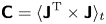 ${\boldsymbol{\mathsf{C}}}=\langle {\boldsymbol{\mathsf{J}}}^\mathrm {T} \times {\boldsymbol{\mathsf{J}}} \rangle _t$, where the superscript ‘T’ denotes the operation of conjugate transpose, and
 $\langle \cdots \rangle _t$ denotes average in time. The matrix
 ${\boldsymbol{\mathsf{C}}}$ is Hermitian so that it possesses real eigenvalues
 $\lambda _n$ and complex eigenvectors
 $\boldsymbol {b}_n(s)$ with orthogonality. Eigenvectors
 $\boldsymbol {b}_n(s)$ (column vectors) are a set of orthogonal spatial bases that serve as the complex spatial principal components – or rather physically the spatial modes – of the complex field
 ${\boldsymbol{\mathsf{J}}}$, while eigenvalues
 $\lambda _n$ represent the energy magnitude of the corresponding spatial principal components. By linearly projecting the complex field
 ${\boldsymbol{\mathsf{J}}}$ onto the spatial bases
 $\boldsymbol {b}_n(s)$, we obtain the temporal principal components
 $\boldsymbol {a}_n(t)$, i.e.
 $\boldsymbol {a}_n(t)={\boldsymbol{\mathsf{J}}}\boldsymbol {b}_n(s)$. The temporal principal components
 $\boldsymbol {a}_n(t)$ (column vectors), therefore, characterize the intensity of the corresponding complex modes
 $\boldsymbol {b}_n(s)$ in time coordinate (Yeaton et al. Reference Yeaton, Ross, Baumgardner and Socha2020). If we designate
 ${\boldsymbol{\mathsf{B}}}=[\boldsymbol {b}_1(s) |\cdots |\boldsymbol {b}_n(s)|\cdots ]$ as the eigenvector matrix and
 ${\boldsymbol{\mathsf{A}}}=[\boldsymbol {a}_1(t)|\cdots |\boldsymbol {a}_n(t)|\cdots ]$ as the temporal principal matrix, the complex field
 ${\boldsymbol{\mathsf{J}}}$ is recovered by
 ${\boldsymbol{\mathsf{J}}}= {\boldsymbol{\mathsf{A}}}{\boldsymbol{\mathsf{B}}}^\mathrm {T}$. In this sense, we can decouple the motion of the film
 $y(t, s)$ into the following form:
 \begin{equation} y(t,s)={{\rm Re}}\Big[ \sum_{n}{\boldsymbol{a}_n(t)\boldsymbol{b}_n^\mathrm{T}(s)} \Big] =\sum_{n}{\alpha_n(t)\zeta_n(s)\cos[\psi_n(t)-\phi_n(s)]}.\end{equation}
In (C1), the relationship between the temporal amplitude  $\alpha _n$, the temporal phase
 $\psi _n$ and the temporal principal component
 $\boldsymbol {a}_n$ is established by
 $\boldsymbol {a}_n(t)=\alpha _n(t)\mathrm {e}^{\mathrm {i}\psi _n(t)}$, and the relationship between the spatial amplitude
 $\zeta _n$, the spatial phase
 $\phi _n$ and the spatial principal component
 $\boldsymbol {b}_n$ is established by
 $\boldsymbol {b}_n(s)=\zeta _n(s)\mathrm {e}^{\mathrm {i}\phi _n(s)}$ (Barnett Reference Barnett1983; Esquivel & Messina Reference Esquivel and Messina2008; Michelin & Doaré Reference Michelin and Doaré2013). With the above decomposition, the salient features of
 $y(s,t)$ are incorporated into its low-order principal components, thereby enabling a reduced-order operation for the dynamical system. For the flapping of the film with
 $L/D=5.0$, its first CEOF mode accounts for more than 99.9 % of the total energy (namely,
 ${\lambda _1}/{\sum _n\lambda _n}>99.9\,\%)$, which is sufficient to furnish the dominant kinematic information on the flapping. For a periodic system with a stable limit cycle, the temporal amplitude
 $\alpha _1$ is almost a constant (Michelin et al. Reference Michelin, Llewellyn Smith and Glover2008), and our focus will be projected on the spatial amplitude
 $\zeta _1$, temporal phase
 $\psi _1$ and spatial phase
 $\phi _1$, as illustrated in figures 17(d) to 17(f), respectively.
Appendix D. Phase-lock POD
For the case of film with  $L/D=5.0$, due to the large-amplitude flapping of the film, the velocity fields are contaminated on a large spatial scale. Thus, the common POD algorithm is not suitable in this situation. A refined algorithm of POD is proposed here in order to achieve the reconstruction of the velocity fields. Considering the pure periodicity of the film flapping, we can readily identify the phase of each frame of the velocity field with Hilbert transform based on the signal of the film deformation, more precisely, the signal of the cross-correlation coefficients from the film's instantaneous deformations. Then, the frames corresponding to the same or similar phase angles are regarded as a set of phase-lock velocity fields. In the present study, one period of the film flapping (360
 $^\circ$) is sequentially split into 60 phase blocks from 0
 $^\circ$ to 360
 $^\circ$, meaning the phase differences within a set of phase-lock velocity fields do not exceed 6
 $^\circ$. Subsequently, POD is applied to each set of the phase-lock velocity fields. The POD modes accounting for 85 % of total energy are utilized to reconstruct the velocity fields in each phase block. Finally, every reconstructed velocity field is put back to its original frame position. The FTLE fields in figure 18 and vorticity fields in figure 22(b) are obtained from the reconstructed velocity fields.
Appendix E. Determining second derivative with optimal quintic smoothing spline
The high-order derivatives of experimental data are ill-posed due to the inescapable noise in the measurement. With the increase of the derivative order, arbitrary tiny noise in the experimental data will generate arbitrary huge divergence in the outcome (Qian et al. Reference Qian, Fu, Xiong and Wei2006b; Nayak Reference Nayak2020). Even for the second derivative, conventional methods such as central differencing and local least squares (Savitzky & Golay Reference Savitzky and Golay1964; Fan & Gijbels Reference Fan and Gijbels1996) also fail to yield satisfactory results. Here, we adopt the derivative method introduced by Epps et al. (Reference Epps, Truscott and Techet2010) to solve the second derivatives of the Fourier coefficients in (3.13) (see § 3.5.2). This method is based on fitting the experimental data to an optimal quintic smoothing spline that is solved by Reinsch's tolerance algorithm (Reinsch Reference Reinsch1967, Reference Reinsch1971; Ahlberg et al. Reference Ahlberg, Nilson and Walsh2016); the derivative of the experimental data will be given by the derivative of the optimal quintic smoothing spline.
A quintic smoothing spline is formed by a set of piecewise-defined quintic polynomial segments joined together. It does not have a specific functional form for the curve. Instead, it estimates the curve for the input data by balancing the fitting error  $E$, and the roughness of the curve
 $R^3$. For the quintic smoothing spline, the fitting error
 $E$ and the roughness
 $R^3$ are, respectively, defined by
 \begin{equation} E(\tilde{f})=\int_x | y(x)-\tilde{f}(x)|^2\,\mathrm{d}\kern 0.06em x,\end{equation}
and
 \begin{equation} R^3(\tilde{f})=\int_{x}\Big|\frac{\mathrm{d}^3\tilde{f}(x)}{\mathrm{d}\kern 0.06em x^3}\Big|^2 \mathrm{d}\kern 0.06em x. \end{equation}
Here, the fitting error  $E(\,\tilde {f})$ measures the distance between the smoothing spline
 $\tilde {f}(x)$ and the original data
 $y(x)$, while the roughness
 $R^3(\,\tilde {f})$ describes the curvature of
 $\tilde {f}(x)$ (Wahba Reference Wahba1990; Ahlberg et al. Reference Ahlberg, Nilson and Walsh2016). The primary principle behind constructing a smoothing spline with Reinsch's tolerance algorithm can be sketched as follows: for a given error tolerance
 $\varXi$, find the smoothest one from the set of the smoothing spline curves that not only fits the original data
 $y(x)$ but adheres to the tolerance limit (Reinsch Reference Reinsch1967, Reference Reinsch1971). Therefore, the determined smoothing spline
 $\tilde {f}(x)$ meets both the following two requirements:
 \begin{equation} [ \mathrm{Minimize }\ R^3 (\,\tilde{f}) ] \land [ E(\tilde{f})\le\varXi ].\end{equation}
For a predetermined tolerance  $\varXi$, the above smoothing spline
 $\tilde {f}(x)$ with the minimum roughness is uniquely determined so that the tolerance
 $\varXi$ and the minimum roughness
 $R^3$ bear a one-to-one correspondence. According to (E3), seeking the optimal smoothing spline
 ${\tilde {f}}_0(x)$ is equivalent to determining the optimal value of the tolerance,
 $\varXi _0$, for the original data. The optimal smoothing spline effectively eliminates data noise while minimizing the deviation from the data so as to achieve a superior balance between the error
 $E(\,\tilde {f})$ and the roughness
 $R^3(\,\tilde {f})$ (Wahba Reference Wahba1990), thus being the optimal approximation of the unknown true value of the data.
Epps et al. (Reference Epps, Truscott and Techet2010) have identified that for the experimental data with a high temporal or spatial resolution, as a set of quintic smoothing splines is constructed utilizing Reinsch's tolerance algorithm by given successive values of tolerance  $\varXi$ (see (E3)), the curve that describes the relationship between the minimum roughness
 $R^3$ of the smoothing splines and the given tolerances
 $\varXi$ possesses a specific form in the
 $\varXi$–
 $R^3$ plane. As the tolerance progressively increases, a distinct kink emerges on the
 $\varXi$–
 $R^3$ curve (refer to figures 28b and 29b), at which the tolerance located is the optimal tolerance
 $\varXi _0$ for the experimental data (Epps et al. Reference Epps, Truscott and Techet2010; Truscott et al. Reference Truscott, Epps and Techet2012). The optimal smoothing spline
 ${\tilde {f}}_0(x)$ determined by
 $\varXi _0$ not only approximates the true value of the original data with excellent accuracy but also ensures the second derivative is well-posed.
Solving the second derivative for the Fourier coefficient  $a_x^0$ in equation (3.13). (ai) The original data of
 $a_x^0$ and its optimal quintic smoothing spline fitting; (aii) magnified view in
 $s/D=1\sim 1.2$ to show the details of data; (aiii) difference between the original data and the smoothing spline fitting, where
 $\delta =a_x^0-\tilde {f}$, which approximately represents the noise in
 $a_x^0$. (b) Roughness,
 $R^3$, versus error tolerance,
 $\varXi$, of quintic smoothing splines solved by iterating Reinsch's tolerance method with a successive value of
 $\varXi$. Here, each point on the curve corresponds to a specific quintic smoothing spline. The optimal error tolerance for the fitting of
 $a_x^0(s)$ is given by the kink on the
 $R^3$–
 $\varXi$ curve as
 $\varXi _0=5.56\times 10^{-12}$. (ci) Comparison of the derivatives solved by the quintic smoothing spline fitting and local least squares; (cii) magnified view in
 $s/D=1.8\sim 2.4$ to show the details. Here, the local least square is solved with the window size of 21 points and the polynomial order of five.

Solving the second derivative for the Fourier coefficient  $a_y^1$ in (3.13). The captions for this figure are the same as those for figure 28 in a one-to-one correspondence. The magnified view, panel (aii), exhibits the details of data in
 $s/D=1.6\sim 1.8$. The optimal error tolerance for the fitting of
 $a_y^1(s)$ is given by the kink on the
 $R^3-\varXi$ curve as
 $\varXi _0=5.49\times 10^{-9}$ in (b). In panel (c), due to the relatively large noise in
 $a_y^1$, its second derivative solved by local least squares is completely divergent, whereas the optimal quintic smoothing spline fitting outputs a satisfactory second derivative of
 $a_y^1$.

With the above method, we can determine the second derivatives of the Fourier coefficients for the reconstructed film motion in (3.13), as well as the subsequent distribution of elastic energy density (see (3.12a,b)). We chose the two representative Fourier coefficients  $a_x^0(s)$ and
 $a_y^1(s)$ as examples for the
 $x$ and
 $y$ directions, respectively, and the solving processes are detailed in figures 28 and 29. For
 $a_x^0(s)$ (figure 28a), to find its optimal quintic smoothing spline fitting, we construct a series of quintic smoothing splines via iterating the Reinsch's tolerance algorithm at 500 predetermined tolerances, which are uniformly and sequentially selected within the range of
 $\varXi ={10}^{-18}\sim {10}^0$ in the logarithmic coordinate of
 $\varXi$, i.e.
 $\log {\varXi }=-18\sim 0$. Since each tolerance
 $\varXi$ corresponds to a specific smoothing spline and thus a specific roughness
 $R^3$, we can obtain a curve of
 $R^3$ versus
 $\varXi$ determined by the 500 tolerance values, as depicted in figure 28(b). Then the optimal tolerance for
 $a_x^0(s)$ is given by the kink on the
 $R^3-\varXi$ as
 $\varXi _0=5.56\times {10}^{-12}$ (the light blue point in figure 28b), with which the optimal quintic smoothing spline for
 $a_x^0(s)$ is constructed, as shown by the dash–dotted line in figure 28(a). By directly taking the analytic second derivative of the quintic smoothing spline, we eventually procure the approximate second derivative for
 $a_x^0(s)$, as shown in figure 28(c). The solution for the second derivative of the coefficient
 $a_y^1(s)$ follows a similar process to that of
 $a_x^0(s)$ except for the optimal tolerance of
 $\varXi _0=5.49\times {10}^{-9}$ (see figure 29b). The optimal quintic smoothing spline for
 $a_y^1(s)$ is compared with the original
 $a_y^1(s)$ in figures 29(ai) and 29(aii). The approximate second derivative for
 $a_y^1(s)$ is shown in figure 29(c) by the dash–dotted line. In the same fashion, we can also procure the approximate second derivatives for the remaining coefficients in (3.13), and the ultimate outcomes have been given in figures 19(c) and 19(d).
In figures 28(c) and 29(c), we also compare the second derivatives determined by quintic smoothing spline fitting with those solved by local least squares (Savitzky & Golay Reference Savitzky and Golay1964; Fan & Gijbels Reference Fan and Gijbels1996). Here, the window size of 21 points and the polynomial order of five are utilized to calculate the local least square. As shown in figure 28(c), even though the noise intensity in  $a_x^0$ is pretty low (figure 28aiii), its second derivative from the local least squares is just barely tolerable, of which the data quality is evidently poorer than the second derivative from the smoothing spline. However, for the coefficient
 $a_y^1$, where the noise intensity (figure 28aiii) is larger than that in
 $a_x^0$ by an order of magnitude (figure 29aiii), the second derivative from the local least squares becomes divergent (figure 29c), whereas the outcome from the quintic smoothing spline is still pretty good. Therefore, we believe that the energy density distribution based on the second derivatives from the quintic smoothing spline fitting is accurate enough, as presented in figure 21.
Appendix F. Additional information for the discussion section (§ 3.6)
Here, an additional figure supporting the results in § 3.6 is presented. Figure 30 shows the motion transition from hybrid flutter to the periodic flapping for the 0.1 mm thick film of  $L/D=5.0$. This transition occurs as the free stream velocity changes from
 $U_\infty =5\ \text {m s}^{-1}$ to
 $U_\infty =6\ \text {m s}^{-1}$. The deflection state and the flection state within the hybrid flutter are presented in figures 30(a) and 30(b), respectively, while the periodic flapping at
 $U_\infty =6\ \text {m s}^{-1}$ is presented in figure 30(c).
Transition of the motion states from hybrid flutter to the periodic flapping for the 0.1 mm thick film with  $L/D=5.0$. Panels (a) and (b) depict the hybrid flutter of the film at
 $U_\infty =5\ \text {m s}^{-1}$ together, where (a) is for deflection state and (b) is for flection state. (c) shows the periodic flapping of the film at
 $U_\infty =6\ \text {m s}^{-1}$.