1. INTRODUCTION
We consider local linear modeling in a time series context under near epoch dependence. Andrews (1995) established uniform convergence with rates for nonparametric density and regression estimators based on the local constant paradigm also under near epoch dependence conditions. The purpose of this study is to provide a central limit theorem for the more desirable class of local linear estimators (Fan and Gijbels, 1996) under similar weak dependence conditions.
Assume that {(Yt,Xt)} is an

-valued stationary sequence (with Yt being

-valued and Xt being

-valued), defined on some probability space

(throughout the paper all the random variables are defined on this space). Among the widely used mixing conditions, such as φ-, ρ-, β-, and α-mixing, α-mixing is no doubt the weakest and most popular in the econometric literature. Under some suitable conditions, the stationary solutions of many time series econometric models (linear or nonlinear) are α-mixing; see, for example, Goródetskii (1977), Pham (1986), Pham and Tran (1985), Tjøstheim (1990), and Tong (1990) on nonlinear autoregressive (AR) models and see Masry and Tjøstheim (1995), Lu (1998), Cline and Pu (1999), Lu and Jiang (2001), Carrasco and Chen (2002), and Saikkonen (2001) on nonlinear autoregressive conditionally heteroskedastic/generalized autoregressive conditionally heteroskedastic (ARCH/GARCH) models. This mixing condition is used extensively in the time series literature (cf. Fan and Yao, 2003). Masry and Fan (1997) establish the asymptotic normality of local polynomial regression estimators under this condition. For reference, its definition is stated as follows.
DEFINITION 0. A stationary sequence {Xt, t = 0, ±1,…} is said to be α-mixing if

as k → ∞, where

and

are two σ-fields generated by {Xt, t ≤ n} and {Xt, t ≥ n + k}, respectively. We call α(·) the mixing coefficient.
However, from a practical point of view, the α-mixing concept suffers from many undesirable features. As Davidson (1994) points out, the following shortcomings are often serious (see also Lu, 2001): (i) even simple autoregressive processes might not be α-mixing and (ii) α-mixing is hard to verify in practice, especially in the case of compound processes. For the former case, Andrews (1984) showed that the stationary solution to a simple linear AR(1) model of the form Xt = ½Xt−1 + et, with et's being independent symmetric Bernoulli random variables taking values −1 and 1, is not α-mixing (but it is near epoch dependent [NED] defined in Definition 1, which follows). For the latter case, the autoregressive moving average (ARMA) process with ARCH/GARCH errors, discussed in Engle (1982) and Weiss (1984) and also Ling and Li (1997), is well applied in financial econometrics, where the model is composed of two time series (ARMA and ARCH/GARCH) models:


where ai and bi are the coefficients in the ARMA(p,q) model, and αi and βi are the coefficients in the GARCH(P,Q) model, with et being independent and identically distributed (i.i.d.) innovation with mean 0 and variance 1. Although the ARCH model and its generalized version, GARCH (see Bollerslev, 1986), have been proved to be α-mixing under some mild conditions (cf. Lu, 1996a, 1996b; Carrasco and Chen, 2002), no results exist to establish whether compound processes are α-mixing. For this reason we use a generalized version of mixing processes, called stable or NED processes, which can easily cover the compounded processes and many nonlinear/non-α-mixing processes. This concept was introduced in Ibragimov (1962) and was developed further by Billingsley (1968) and McLeish (1975a, 1975b, 1977). It has been used extensively in econometrics following Bierens (1981); see, for example, Gallant (1987), Gallant and White (1988), and Andrews (1995). Lu (2001) established asymptotic normality for kernel density estimators under this condition. Nze, Bühlmann, and Doukhan (2002) and Nze and Doukhan (2004) have investigated an alternative class of dependent processes they call “weak dependent.”1
Let E be some normed measurable space with norm ∥·∥, for example, the Euclidean space

with the Euclidean norm and D = 1 + d in the setting of this paper. An E-valued stochastic sequence

is called

-weak dependent (cf. Nze et al., 2002, p. 399) if for some monotone sequence

decreasing to zero at infinity and some real-valued function ψ with arguments

,

for any u-tuple (i1,…, iu), any v-tuple (j1,…, jv) with i1 ≤ ··· ≤ iu < iu + r ≤ j1 ≤ ··· ≤ jv and all

, where

,

, and

. Here

is the set of measurable bounded functions on Eu and set

for

, and Lip(h) = supx≠y|h(x) − h(y)|/∥x − y∥1 is the Lipschitz modulus of a function

with respect to the [ell ]1-norm in Eu, defined by ∥x∥1 = ∥(x1,…, xu)∥1 = ∥x1∥ + ··· + ∥xu∥ for x ∈ Eu.
Let Yt and Xt be both stationary processes,

- and

-valued, respectively, defined based on a stationary process {εt} by


where Xτ denotes the transpose of X (a vector or matrix),

and

are two Borel measurable functions, respectively, and {εt} may be vector-valued. Let ν > 0 be a positive real number.
DEFINITION 1. The stationary process {(Yt,Xt)} is said to be near epoch dependent in Lν norm (NED in Lν for simplicity) with respect to a stationary α-mixing process {εt} if

as m → ∞, where |·| and ∥·∥ are the absolute value and the Euclidean norm of

, respectively, Yt(m) = ΨY,m(εt,…, εt−m+1), Xt(m) = (Xt1(m),…, Xtd(m))τ = ΨX,m(εt,…, εt−m+1), and ΨY,m and ΨX,m are

- and

- valued Borel measurable functions with m arguments, respectively. We will call vν(m) the stability coefficients of order ν of the process {(Yt,Xt)}.
Clearly, {(Yt(m),Xt(m))} is an α-mixing process with mixing coefficient

The type of setting where our results are useful is for models with complicated dynamics in both mean and variance for which the usual mixing conditions do not necessarily apply. These sorts of models are common in finance and economics, and near epoch dependence is sometimes easier to verify in the case of these models.
Our limiting results will resemble conventional limiting results for local linear estimators under more standard conditions. That is, under some restrictions on α(k) and vν(m) we obtain the optimal pointwise rate of convergence for i.i.d. data (Stone, 1980) along with the same asymptotic distribution that would obtain were the data i.i.d. with the same marginal distribution. This type of result is to be contrasted with those obtained by Phillips and Park (1998) and Karlsen and Tjøstheim (2001) for unit root or null recurrent processes (for near-integrated processes, see also Bandi, 2004) for which the rates of convergence are slower and limiting distributions are nonnormal. Moloche (2000) also discusses local polynomial estimation for recurrent diffusions.
In the next section we define the setting and estimator we shall examine. The main asymptotic results are given in Section 3. In Section 4 we provide some numerical results based on some common econometric models.
2. METHODOLOGY
2.1. Notation and Main Assumptions
We summarize here the main assumptions we are making on the data generating process (DGP) (1.6) and the kernel K to be used in the estimation method. Assumptions (A1)–(A4) are related to the nonlinear process itself.
(A1) The DGP is a strictly stationary NED process (cf. (1.6)), with order ν = 2 + δ/2, with respect to the α-mixing process {εt}, where the constant δ > 0 is specified in Assumption (A2), which follows. For all i and j in

, the vectors Xi and Xj admit a joint density fij; moreover, fij(x′,x′′) ≤ C for all

, all

, where C > 0 is some constant, and f denotes the marginal density of Xi.
(A2) The random variable Yi has finite absolute moment of order (2 + δ), that is, E[|Yi|2+δ] < ∞ for some δ > 0.
(A3) (i) The regression function g(x) = E(Yt|Xt = x) is twice differentiable. Denoting by g′(x) and g′′(x) its gradient and the matrix of its second derivatives (at x), respectively, x [map ] g′′(x) is continuous at x. (ii) The density function f (x) is continuous at x. (iii) The conditional variance function Var(Yt|Xt = x) is continuous at x.
Assumption (A4) is an assumption of the mixing coefficients.
(A4) For the mixing coefficient of εt, the function α is such that

Assumption (A5) deals with the kernel function

, to be used in the estimation method. For any

, define

(A5)
(i) For any

, |Kc(u)| is uniformly bounded by some constant Kc+ and is integrable:

.
(ii) For any

, |Kc| has an integrable second-order radial majorant; that is, QcK(x) := sup∥y∥≥∥x∥[∥y∥2Kc(y)] is integrable.
(iii) For any

, Kc is Lipschitz continuous of order 1; that is, for some constant C > 0,

This assumption allows an unbounded support for the kernel function; compare this with Condition 2(i) of Masry and Fan (1997, p. 170), who require the kernel function to have a bounded support.
Throughout, we assume that the observations of the NED process {(Yt,Xt)} are (Yt,Xt), t = 1,2,…,T. For convenient reference, we list here some conditions on the asymptotic behavior, as T → ∞, of the bandwidth bT that will be used in the discussion that follows (cf. Lemma 3.4). Assumption (B1), which follows, is standard, whereas Assumptions (B2)–(B4) look complex: some simple and verifiable conditions on the stability and mixing coefficients to ensure that they hold will be given in the main theorem (Theorem 3.1) and its corollary (Corollary 3.1).
(B1) The bandwidth bT tends to zero in such a way that TbTd → ∞ as T → ∞.
(B2) There is a positive integer m = mT → ∞ such that the stability coefficients, defined in (1.6) with ν = 2 and ν = 2 + δ/2, satisfy

and

(B3) There exist two sequences of positive integer vectors,

and

, with m = mT → ∞ such that p = pT = o((TbTd)1/2), q/p → 0 and T/p → ∞, and Tp−1α(m) → 0.
(B4) bT tends to zero in such a manner that qbTd = O(1) such that

Remark. Assumption (B1) is standard on the bandwidth, the same as in the i.i.d. case; Assumption (B2) is concerned with the conditions on the stability coefficients related to the bandwidth; and Assumptions (B3) and (B4) are on the mixing coefficients that are associated with the bandwidth, among which (B3) together with (B1) is similar to the conditions specified for the strongly mixing processes in Condition 3 of Masry and Fan (1997, p. 172). Assumptions (B2)–(B4) are phrased as restrictions on the decay rates of the stability and mixing coefficients for a given bandwidth, although one could rewrite these conditions as restrictions on the bandwidth (and hence the implied rate of convergence of the estimator) for a given decay rate, thereby allowing greater dependence at the cost of slower convergence. Although Assumptions (B2)–(B4) look somewhat complex, some milder and more specific conditions can be derived from them with the bandwidth set as a power function of the number of observations, as is generally the case in practice. For the details, see Theorem 3.1 together with Corollary 3.1 and the remark there in Section 3.
2.2. Least Squares Local Linear Fitting
Although the Nadaraya–Watson method is central in most nonparametric regression methods in the traditional i.i.d. series case, it has been well documented (see, e.g., Fan and Gijbels, 1996) that this approach suffers from several severe drawbacks, such as poor boundary performances, excessive bias, and low efficiency and that the local polynomial fitting methods developed by Stone (1977) and Cleveland (1979) are generally preferable. Local polynomial fitting, and particularly its special case—local linear fitting—have become increasingly popular in the light of recent work by Cleveland and Loader (1996), Fan (1992), Fan and Gijbels (1992, 1995), Hastie and Loader (1993), Ruppert and Wand (1994), and several others. Masry and Fan (1997) have studied the asymptotics of local polynomial fitting for regression under general α-mixing conditions; see also Fan and Yao (2003). In this paper, we extend this approach to the context of our generalized mixing dependence NED processes by defining an estimator of g based on local linear fitting and establishing its asymptotic properties.
The idea of local linear fitting consists of approximating, in a neighborhood of x, the unknown function g by a linear function. Under Assumption (A3), we have

Locally, this suggests estimating (a0,a1τ) = (g(x),g′(x)), hence constructing an estimator of g from

where bT is a sequence of bandwidths tending to zero at appropriate rate as T tends to infinity and K(·) is a (bounded) kernel with values in

.
In the classical i.i.d. and time series case, the solution of the minimization problem (2.3) is easily shown to be

, where

is an n × (d + 1) matrix with ith row (1,bT−1(Xi − x)τ),

diag(K((X1 − x)/bT),…, K((XT − x)/bT)), and

(see, e.g., Fan and Gijbels, 1996). In the generalized NED series case, though such an expression still holds, we instead write the solution to (2.3) in the following form, which is very convenient for the purpose of characterizing its limiting distribution:

with (letting ((Xj − x)/bT)0 := 1)

and

It follows that

where

and Zj := Yj − a0 − a1τ(Xj − x).
The organization of the paper is as follows. If, under adequate conditions, we are able to show that conditions (C1)–(C3) (to be presented subsequently) apply, then (2.4) and Slutsky's classical argument imply that, for all x (all quantities involved indeed depend on x),

This asymptotic normality result (with explicit values of μT, Σ, and U), under various forms (depending on the stability assumption, the mixing assumption, the choice of the bandwidth bT, etc.), is the main contribution of this paper; see Theorem 3.1 and its Corollary 3.1.
Conditions (C1)–(C2) are now presented.
(C1) (TbTd)1/2(WT − EWT) is asymptotically normal,
(C2) (TbTd)1/2(EWT − μT)→ 0 and Var((TbTd)1/2WT) → Σ for some positive definite matrix Σ, and
(C3)

for some nonsingular matrix U.
2.3. Approximations
A fundamental technique that will be widely used to study (C1)–(C3) is the following approximation to the NED process {(Yt,Xt)} by the α-mixing process {(Yt(m),Xt(m))} defined in Definition 1, that is,


where

and the mixing coefficients of {(Yt(m),Xt(m))} satisfy

with α(·) defined in Definition 0.
On the basis of (2.6) and (2.7), we can construct the approximations to UT and WT, respectively, by

with (letting ((Xj(m) − x)/bT)0 := 1)

and

and Zj(m) := Yj(m) − a0 − a1τ(Xj(m) − x).
We have the following lemma on the approximations.
LEMMA 2.1. Let m = mT be a positive integer tending to ∞ and L = LT a positive real number tending to ∞ as T → ∞. Then under Assumptions (A2) and (A5), as T → ∞,


for i, [ell ] = 0,1,…, d.
Proof. See Section A.2 in the Appendix.
3. ASYMPTOTIC RESULTS
We begin with some preliminaries on the asymptotic bias and variance.
3.1. Preliminaries
Claim (C3) is easily established from the following lemma, the proof of which is similar to that of Lemma 3.2, which follows, and is therefore omitted.
LEMMA 3.1. Assume that Assumptions (A1), (A4), and (A5) hold and that bT satisfies Assumptions (B1) and (B2). Then

as T → ∞.
The remainder of this Section 3.1 is devoted to claim (C2). The usual Cramér–Wold device will be adopted. For all

, let

with Kc(u) defined in (2.1). The following lemma provides the asymptotic variance of AT for all c and hence that of (TbTd)1/2WT.
LEMMA 3.2. Assume that Assumptions (A1), (A2), (A3)(ii) and (iii), (A4), and (A5) hold and that bT satisfies Assumptions (B1) and (B2). Then

where

Hence, limT→∞ Var((TbTd)1/2WT) = Σ.
Proof. See Section A.2 in the Appendix.
Next, we consider the asymptotic behavior of E[AT].
LEMMA 3.3. Assume that Assumptions (A3)(i) and (ii) and (A5) hold. Then

where

Proof. The proof is routine and is omitted.
3.2. Asymptotic Normality
The asymptotic normality of our estimators relies on the following lemma (see (2.5) for the definition of WT(x)).
LEMMA 3.4. Suppose that Assumptions (A1), (A2), (A3)(ii) and (iii), (A4), and (A5) hold with f (x) > 0 and that the bandwidth bT satisfies conditions (B1)–(B4). Denote by σ2 the asymptotic variance (3.1). Then (TbTd)1/2(cτ[WT(x) − EWT(x)]/σ) is asymptotically standard normal as T → ∞.
Proof. See Section A.3 in the Appendix.
We now turn to the main consistency and asymptotic normality result.
THEOREM 3.1. Let Assumptions (A1), (A2), (A3), and (A5) hold, with f (x) > 0, v2+δ/2(x) = O(x−μ), and α(x) = O(x−λ) for some μ ≥ max{4(κ1 − 1),κ3 /(1 + δ/4)}κ2 and some λ > (a + 1)(1 + 4/δ) with a > δ/(4 + δ), such that T2+4/δbTμ/κ2−κ1 → 0, TbT[1+2/{a(1+4/δ)}]d/log T → ∞, and TbT[2λ/{a(1+4/δ)}−1]dlog T → 0 as T → ∞, where κ1 = 2 + d + 2d/δ, κ2 = a(1 + 4/δ)(1 + δ/4)/d, and κ3 = 2 + 2d + δ/2 + 4d/δ. Then,

as T → ∞, where U, Σ, and B0(x) and B1(x) are defined in Lemmas 3.1, 3.2, and 3.3, respectively.
If furthermore the kernel K(·) is a symmetric density function, then (3.3) can be strengthened to

(so that gT(x) and gT′(x) are asymptotically independent), where

and

Proof. See Section A.3 in the Appendix.
From this theorem, we can derive the following corollary, which gives the conditions under which the usually used optimal bandwidth, bT = O(T−1/(4+d)), is achievable.
COROLLARY 3.1. Let Assumptions (A1)–(A3) and (A5) hold with f (x) > 0, v2+δ/2(x) = O(x−μ), and α(x) = O(x−λ) for some μ ≥ max{4(κ1 − 1),κ3 /(1 + δ/4),(κ4 + κ1)}κ2 and some λ > max{(a + 1),a(1 + 2/d)}(1 + 4/δ) with a > max{1,d/2}δ/(4 + δ), and bT = O(T−1/(4+d)), where κ1, κ2, and κ3 are specified in Theorem 3.1 and κ4 = (4 + d)(2 + 4/δ). Then the conclusion of Theorem 3.1 holds.
Proof. See Section A.3 in the Appendix.
Remark.
(i) In Theorem 3.1 and Corollary 3.1, the positive constants μ and λ specify the decay rates for the stability and mixing coefficients tending to zero (the larger μ and λ, the faster the decay rates), which are related to the positive constant δ determining the moment order of Yt. For example, if we let a = 2dδ/(4 + δ) and d = 1 in Corollary 3.1, then simple calculation leads to the requirement that μ > 37 + 6.5δ + 44/δ and λ > max{3 + 4/δ,6}. Therefore, when μ and λ are sufficiently large, δ can be equal to a small number close to zero. This condition is automatically satisfied when both the stability and mixing coefficients decay at geometric rates (cf. the examples in Section 4).
(ii) When the model (1.2) with (1.3) being an integrated GARCH model is considered, then the second-order moments of Yt are unavailable, for which the asymptotic normality for the estimates stated in Theorem 3.1 and Corollary 3.1 cannot be ensured but the consistency of the estimates is still obtainable if E|Yt| < ∞ holds.
The asymptotic distribution is as if the sequence (Yj,Xj) were i.i.d. with the same marginal distributions. That these results are expected for such weakly dependent stationary processes as ours has already been shown by Masry and Fan (1997) for α-mixing processes. By contrast, for nonstationary or strongly dependent time series slower convergence rates and even nonnormal limiting distributions can hold; see Phillips and Park (1998), Karlsen and Tjøstheim (2001), and Bandi (2004). Consistent standard errors can be computed by estimating the conditional variance and marginal covariate density. For the conditional variance we can use that Var(Yj|Xj = x) = E(Yj2|Xj = x) − E2(Yj|Xj = x) and then compute the additional regression estimator of E(Yj2|Xj = x). We can estimate the marginal density by the kernel estimator (UT)00 defined earlier. Consistency of the standard errors follows under our conditions.
The optimal bandwidth can be found using the same formula given in Masry and Fan (1997, Sect. 3.1). The practical choice of the bandwidth can be made by the conventional cross-validation (CV) rule, which is often computationally intensive, especially for large sample size, or the generalized cross-validation (GCV) rule of Wahba (1977) and Craven and Wahba (1979) for less intensive computation. In Section 4, we use the bandwidth selected by GCV in the simulations and by CV in the empirical application.
One of the important advantages of local polynomial (and linear) fitting over the more traditional Nadaraya–Watson approach is that it has much better boundary behavior. This advantage often has been emphasized in the usual regression and time series settings when the regressors take values on a compact subset of

. For example, as Fan and Gijbels (1996) and Fan and Yao (2003) illustrate, for a univariate regressor X with bounded support ([0,1], say; here, d = 1), it can be proved, using an argument similar to the one we are developing in the proof of Theorem 3.1, that asymptotic normality still holds at the boundary point x = cbT (here c is a positive constant) but with asymptotic bias and variance

and

4. NUMERICAL RESULTS
4.1. Simulation
In this section we report the results of a small Monte Carlo study of the method described in this paper, the purpose of which is to illustrate that local linear estimates with a conventional choice of bandwidth as pointed out by Masry and Fan (1997) for α-mixing processes can work reasonably well for the processes for which α-mixing is not guaranteed but near epoch dependence is satisfied.
Model 1 (AR(1)-GARCH(1) model).
In financial econometrics, a commonly used model is the following compound model:


where rt is the daily return of some equity on day t, modeled by an AR(1) model, (4.1), and ht is the conditional variance of rt, given the past information up to day t − 1, modeled by a GARCH(1,1) model, (4.2), with α0 > 0, α1 ≥ 0, β1 ≥ 0, and {et} being an i.i.d. random sequence with Eet = 0 and Eet2 = 1 (taken to be standard normally distributed in this example). This is a special case of the general ARMA(p,q)-GARCH(P,Q) model given in (1.2) and (1.3).
If |a| < 1, it is well known that model (4.1) can be expressed as

and under α1 + β1 < 1 with some suitably regular conditions (cf. Carrasco and Chen, 2002), the εt in the GARCH(1,1) model (4.2) is strongly (α-) mixing with a geometrically decaying mixing coefficient. Here it is difficult to show under such natural and mild conditions |a| < 1 and α1 + β1 < 1 (to the best of our knowledge) that rt is strongly (α-) mixing, but it can be shown that rt is NED of order 2 + δ with respect to a strongly (α-) mixing process, if E|εt|2+δ < ∞, with stable coefficients (because of the convex property of |·|2+δ)

decaying at a geometric rate, where

and

. Here the conditions to ensure E|εt|2+δ < ∞ can be found in Carrasco and Chen (2002), and therefore E|rt|2+δ < ∞ can be guaranteed.
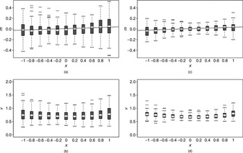
We are concerned with estimation of the autoregression function m(x) = E(rt|rt−1 = x) = a0 + ax and the conditional variance function v(x) = E((rt − m(x))2|rt−1 = x), where our theory developed in this paper applies obviously whereas the theory based on the strong (α-) mixing in the literature would not do if rt is non-strongly mixing. The box plots of the local linear estimators of m and v, based on 100 replications with each sample size equal to 100 and 500, are depicted in Figures 1a–d, respectively, where et is with standard normal distribution, and as suggested by a referee, we took the parameters a0 = 0.001682, a = 0.020602, α0 = 0.137526, α1 = 0.094518, and β1 = 0.726777, which are the parameter estimates of the model (4.1) with (4.2) obtained from the real data of the FT100 Index given in Section 4.2 by the maximum likelihood method procedure in the GARCH module of S-plus. In the simulations, the bandwidth bT was chosen by the conventional generalized cross-validation rule of Wahba (1977) and Craven and Wahba (1979).

Simulation for Model 1—Box plots of the local linear fitting for the conditional mean and conditional variance of 100 replications of the linear AR(1)-GARCH(1,1) model (Model 1) with a0 = 0.001682, a = 0.020602, α0 = 0.137526, α1 = 0.094518, and β1 = 0.726777, and et ∼ N(0,1), for different sample sizes: (a) conditional mean m(x) = E(rt|rt−1 = x) = a0 + ax, sample size = 100, (b) conditional variance v(x), sample size = 100, (c) conditional mean m(x) = E(rt|rt−1 = x) = a0 + ax, sample size = 500, and (d) conditional variance v(x), sample size = 500. In (a) and (c), the solid line stands for the true conditional mean m(x) = a0 + ax.
Overall, the simulation results in the example of Model 1 adapt very well to our asymptotic theory: with the sample size increasing, the local linearly estimated curves with a conventional choice of bandwidth become more stable and fit better to the actual curve lines both for the conditional mean and conditional variance functions; see Figures 1a and c for the estimates of the conditional mean, which are compatible with the actual line in Model 1, and Figures 1b and d for the estimates of the conditional variance. The sample size equal to 500 seems to work very well in all cases.
4.2. An Empirical Application
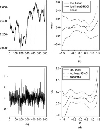
We investigate the UK FT100 Index, with sample size 602, from January 1, 1990, to April 21, 1992, for an illustration. In Figure 2, the index series Pt and the return series rt, defined by

are plotted in Figures 2a and b, respectively. The local linear estimates of the conditional mean m(x) = E(rt|rt−1 = x) and the conditional variance function v(x) = E((rt − m(x))2|rt−1 = x) together with the 95% confidence intervals based on the asymptotic normality in Section 3 are plotted in Figures 2c and d, where the bandwidths used for the conditional mean and conditional variance are 0.34 and 0.5, respectively, chosen by the cross-validation rule. In addition the estimates of the following parametric linear model:

with et the same as before, leading to

and

, are also plotted in Figures 2c and d, respectively, where the estimated parameters are

,

,

, and

.

Real example—The local linear fitting for the conditional mean and conditional variance of the return series of the UK FT100 Index from January 1, 1990, to April 21, 1992, with 602 observations: (a) FT100 Index series, (b) return series of FT100 Index, (c) conditional mean, and (d) conditional variance. The dashed lines in (c) and (d) are the estimated linear mean and quadratic variance functions, respectively, from the parametric linear model (4.3).
From Figures 2c and d, we can observe that both the conditional mean and conditional variance functions appear to be nonlinear. Roughly, the conditional mean first increases before x around −0.4, then decreases between −0.4 and around 0.7, and increases again when x > 0.7. Correspondingly, the conditional variance mostly follows a similar pattern to that of the conditional mean, increasing with x when x < −0.75 and x > 0.8 and decreasing with x when 0.25 < x < 0.9, which appears to be consistent with the “high return, high risk” rule, but the pattern is completely different from that of the conditional mean when −0.75 < x < 0.25, which looks to be of “U” shape as observed in Figure 1d in the simulation example. However, the pointwise standard errors reveal that the mean effect is never significantly different from the linear, whereas the variance effect is only rarely different from a quadratic function.
APPENDIX: Proofs
A.1. Some Basic Lemmas.
The proof of the main results relies on some intermediate results. The first one is a lemma borrowed from Ibragimov and Linnik (1971) or Deo (1973), where we refer for a proof.
LEMMA A.1.
(i) Let

denote the class of

-measurable random variables ξ satisfying ∥ξ∥r := (E|ξ|r)1/r < ∞. Let

and

. Then, for any 1 ≤ r,s,h < ∞ such that r−1 + s−1 + h−1 = 1,

where

.
(ii) If moreover |X| and |Y | are P-a.s. bounded, the right-hand side of (A.1) can be replaced with

.
The following lemma establishes the relationship between the related quantities based on the original samples (Xi,Yi) and on the approximated α-mixing samples (Xi(m),Yi(m)), which will play important roles throughout the proofs that follow.
LEMMA A.2. Let m = mT be a positive integer tending to ∞ as T → ∞. Then under Assumptions (A2) and (A5), it holds that for any positive real number L = LT tending to ∞, as T → ∞,


for i ≠ j,

and for any 0 < δ′ < δ,

where O(·) and o(·) hold uniformly with respect to x.
Proof. We prove (A.2)–(A.5) one by one. To prove (A.2), note first that

Here, using the bounded property of the kernel function K(·),

Next, let Yi,L = Yi I{|Yi|≤L} and Yi,U = Yi I{|Yi|>L}, where IA is an indicator function of set A. Then

where, as a result of |EYi,U K((x − Xi)/bT)| = o(L−(1+δ)) as T → ∞ (in an argument similar to (A.11), which follows),

because of the Lipschitz continuity of the kernel function K(·),

using the boundedness of K(·),

Then it follows from (A.8) together with (A.9)–(A.11) that

Finally, (A.2) follows from (A.6) together with (A.7) and (A.12).
The proof of (A.3) can be proved in an argument similar to that in the preceding discussion. First,

Here, similarly to (A.7) by the boundedness of K(·),

again by the boundedness of K(·) together with Cauchy inequality,

Next,

where, similarly to (A.11),

as a result of |EYi,U2K2((x − Xi)/bT)| = o(L−δ) (the same argument as (A.16)),

the same argument as (A.10) leads to

and

Finally, (A.3) follows from (A.13)–(A.19).
For (A.4), first note that

Here, similarly to (A.7), by the boundedness of K(·), and then by Cauchy inequality,

again,

Next,

where, by Assumption (A2) and the assumed properties of K(·) in Assumption (A5),

and similarly,

Finally, (A.4) follows from (A.20)–(A.25).
For the proof of (A.5), by noting that

with YK1 = (Yt(m) − Yt)K((x − Xt(m))/bT), YK2 = Yt{K((x − Xt(m))/bT) − K((x − Xt)/bT)}, and YK3 = Yt K((x − Xt)/bT), it follows that

where E|YK1|2+δ′ ≤ C|Yt(m) − Yt|2+δ′ ≤ Cv2+δ′(m) and

and hence (A.5) holds. █
To cope with the approximation terms of UT(m) and WT(m) defined in Section 2.3, we will need the following lemma, termed the cross term lemma, which is of independent interest and will play important roles in the proofs of the theorems that follow.
LEMMA A.3. (Cross term lemma). Let {(Zj(m),Xj(m)); 1 ≤ j ≤ q} be a stationary sequence with mixing coefficient

and set

, where

is a kernel function satisfying Assumption (A5). Denote by Δj(m)(x) = ηj(m)(x) − Eηj(m)(x),

. Then, for any positive integer cT,

where

and

Proof. First, we note that

Then applying Lemma A.2,


Therefore it follows from (A.28)–(A.30) that (taking L = bT−2d/δ)

therefore,

On the other hand, for i < j, by Lemma A.1(i) with r = s = 1/(2 + δ′) and (A.5) of Lemma 5.2 and then taking L = bT−2d/δ and δ′ = δ/2,

therefore,

The result of this lemma therefore follows from (A.32) and (A.34). █
A.2. Proof for Sections 2 and 3.1.
Proof of Lemma 2.1. Denote by Ki(x) = (x)i K(x). Then it can be noted that

which is the desired result. █
Proof of Lemma 3.1. This lemma easily follows from Lu (2001); see also the proof of Lemma 3.2. The detail is omitted. █
Proof of Lemma 3.2. Set ηj = Zj Kc((Xj − x)/bT) and Δj = ηj − Eηj. Then we note that AT defined in Section 3.1 can be expressed as

and therefore

It easily follows from the Lebesgue density theorem (see Devroye and Györfi, 1985, Ch. 5) that the first term of (A.36) is convergent to the right-hand side of (3.1). Therefore, to complete the proof of this lemma, it suffices to show that AT 2 → 0 as T → ∞. By noting that EΔi Δj = EΔi(m)Δj(m) + EΔi(m)(Δj − Δj(m)) + E(Δi − Δi(m))Δj, we can further separate AT 2 into three parts: AT 2 = AT 21 + AT 22 + AT 23, where, by Lemma A.3 (taking q = T and cTa = bT−δd/(4+δ)) together with Assumption (B2),

by Assumption (A4);

and as a result of E(Δi(m))2 ≤ E(ηj(m))2 = O(bTd) + O(bT−2−2d/δv2(m)) + O(bT−1−2d/δv21/2(m)) + o(bTd) = O(bTd), following from (A.3) of Lemma A.2 with L = bT−d/δ and the condition (B2), and, by using the Lipschitz continuity and boundedness of the kernel K(·) and taking

,

we have

and similarly to AT 22, it can be proved that

The proof of the lemma is completed. █
A.3. Proofs for Section 3.2.
Proof of Lemma 3.4. The fundamental idea to prove the asymptotic normality of WT(x) is to divide WT(x) into two parts: with m = mT → ∞ (to be specified later),

where WT(m)(x) is defined in Section 2.3. Then applying the approximation lemma (Lemma 2.1) with L = LT = (TbT−d)1/[2(1+δ)],

following from Assumption (B2); and similarly

Therefore, to have the conclusion of this lemma, it suffices to prove that

is asymptotically standard normal as T → ∞, which is the main effort we will make in this paper.
Recalling

define ζTj(m) := bT−d/2Δj(m) and let

. Then,

where

Now, let us decompose T−1/2ST(m) into smaller pieces involving “large” and “small” blocks. More specifically, consider

where p = pT and q = qT are specified in Assumption (B3). Without loss of generality, assume that, for some integer r = rT, T is such that T = r(p + q), with r → ∞. For each integer 1 ≤ i ≤ 2, define

Clearly ST(m) = ϒ(m)(T,x,1) + ϒ(m)(T,x,2). Note that ϒ(m)(T,x,1) is the sum of the random variables ζTi(m) over “large” blocks, whereas ϒ(m)(T,x,2) are sums over “small” blocks. If it is not the case that T = r(p + q) for some integer r, then an additional term ϒ(m)(T,x,3), say, containing all the ζTj(m)'s that are not included in the large or small blocks, can be considered. This term will not change the proof much. The general approach consists of showing that, as T → ∞,


for every ε > 0. Note that

The term ϒ(m)(T,x,2)/(σT1/2) is asymptotically negligible by (A.42). The random variables U(m)(1,T,x,j) are asymptotically mutually independent by (A.41). The asymptotic normality of ϒ(m)(T,x,1)/(σT1/2) follows from (A.43) and the Lindeberg–Feller condition (A.44). The lemma thus follows if we can prove (A.41)–(A.44). This proof is given subsequently. The arguments are reminiscent of those used by Robinson (1983), Masry (1986), and Nakhapetyan (1987), but, differently from those references, because of m = mT depending on T in the α-mixing process {(Yt(m),Xt(m))}, the details become much more complex and involved (cf. Lu, 2001) and heavily depend on Lemmas 2.1 and A.3 established previously.
Proof of (A.41). Let

The distance,

, between two distinct sets

and

is at least q if j ≠ j′. Clearly,

is the set of indices involved in U(m)(1,T,x,j), which contains p indices.
Let aj := exp{iuU(m)(1,T,x,j)}, where i2 = −1. Note that

Because |E[aj]| ≤ 1,

Note that d(I[ell ],Ij) ≥ q for any [ell ] ≠ j, and set q = 2m. It follows by applying Lemma A.1(ii) to each term on the right-hand side that

which tends to zero by condition (B3). █
Proof of (A.42). For notational simplicity, refer to the random variables U(m)(2,T,x,j), j = 0,1,…, r − 1, as

. We have

Because Xn is stationary (recall that ζTj(m)(x) := bT−d/2Δj(m)(x)),

From (A.3) and the Lebesgue density theorem (see Devroye and Györfi, 1985, Ch. 2), and then taking L = bT−d/δ,

where the final equality follows from bT−2−d−2d/δv2(m) ≤ bT−2−2d−4d/δv2(m) ≤ bT−4(1+d+2d/δ)v2(m) = O(1) by Assumption (B2).
We need the cross term lemma, Lemma A.3, for

. Thus, applying Lemma A.3 together with (B2) and then taking cT = q yields

It follows from Assumption (B4) that πT = O(1) and

Set

Then

. Because p > q, if i and i′ belong to two distinct sets

and

, then |i − i′| > q. In view of (A.45) and (A.33) and then Assumption (B2), we obtain

Condition (B4) implies that qbTd = O(1) and πT = O(1). Thus, from (A.45), (A.47), and (A.48),

which tends to zero by q/p → 0 and condition (B4); (A.42) follows. █
Proof of (A.43). Let ST(m)′ := ϒ(m)(T,x,1) and ST(m)′′ := ϒ(m)(T,x,2). Then ST(m)′ is a sum of ζj(m)'s over the “large” blocks, ST(m)′′ over the “small” ones. Lemma 3.2 and its argument together with Lemma A.2 imply T−1E[|ST(m)|2] → σ2. This, combined with (A.42), entails T−1E[|ST(m)′|2] → σ2. Now,

where

. Observe that (A.43) follows from (A.49) if the last sum in the right-hand side of (A.49) tends to zero as T → ∞. Using the same argument as in the derivation of the bound (A.45) for

, this sum can be bounded by

which tends to zero by condition (B4). █
Proof of (A.44). We need a truncation argument because Zi(m) is not necessarily bounded. Set Zi(m)M := Zi(m)I{|Zi(m)|≤M}, ηi(m)M := Zi(m)MKc((Xi(m) − x)/bT), Δi(m)M := ηi(m)M − Eηi(m)M, ζTi(m)M := bT−d/2Δi(m)M, where M is a fixed positive constant, and define

. Put

Clearly, |ζTi(m)M| ≤ CMbT−d/2. Therefore |U(m)M(1,T,x,j)| < CMpbT−d/2. Hence

Now, U(m)M(1,T,x,j)/(σT1/2) ≤ Cp(TbTd)−1/2 → 0, because of Assumption (B3). Thus P[U(m)M(1,T,x,j) > εσT1/2] = 0 at all j for sufficiently large T. Thus Q4(m)M = 0 for large T, and (A.44) holds for the truncated variables. Hence,

where σM2 := Var(ZiM|Xi = x) f (x)∫Kc2(u) du and ZiM = Zi I{|Zi|≤M}.
Defining

, we have ST(m) = ST(m)M + ST(m)M*. Note that

Letting T → ∞, E1 tends to zero by (A.50) and the dominated convergence theorem. Letting M go to infinity, the dominated convergence theorem also implies that σM2 := Var(ZiM|Xi = x) f (x)∫Kc2(u) du converges to

and hence that E3 tends to zero. Finally, to prove that E2 also tends to zero, it suffices to show that ST(m)M*/T1/2 → 0 in probability as first T → ∞ and then M → ∞, which in turn would follow if we could show that

This follows along the routine argument of Lemma 3.3 together with Lemma A.2. The proof of Lemma 3.4 is thus complete. █
Proof of Theorem 3.1. We establish that the bandwidth conditions (B1)–(B4) hold. First, Assumption (B1) holds clearly by the condition TbT[1+2/{a(1+4/δ)}]d/log T → ∞.
Next, take m = mT = [lfloor ]bT−δd/{a(4+δ)}[rfloor ] and q = 2m, where [lfloor ]a[rfloor ] stands for the integer part of a. Then it easily follows from Assumption (A4) that (B4) holds.
On the other hand, note that v2+δ/2(m) = O(m−μ) implies v2(m) = O(m−μ/(1+δ/4)).

which tends to zero by the condition of this theorem;

which is deduced by the condition μ ≥ 4(κ1 − 1)κ2; and

which is deduced by the condition μ ≥ κ2κ3 /(1 + δ/4). Therefore Assumption (B2) holds.
Set p = (TbTd/log T)1/2. Then p = o((TbTd)1/2) and T/p = {T log T/bTd}1/2 → ∞ clearly; and

and

by the conditions of this theorem. Therefore Assumption (B3) holds.
Finally, as α(x) = O(x−λ) for some λ > (a + 1)(1 + 4/δ) with a > δ/(4 + δ),

as k → ∞. Therefore Assumption (A4) holds. The theorem thus follows from Lemmas 3.1–3.4. █
Proof of Corollary 3.1. This corollary easily follows by checking the conditions on the bandwidth in Theorem 3.1. The detail is omitted. █