1. INTRODUCTION
Since the work by Dickey and Fuller (1979, 1981), integration testing has become routine in empirical studies to discriminate between time series integrated of order one or zero, I(1) or I(0). The persistence in many economic and financial time series, however, is not well captured by the I(1)/I(0) model. This led to the long memory paradigm introduced to econometrics by Granger and Joyeux (1980); see Henry and Zaffaroni (2003) for a recent review. Most often, long memory is modeled by fractionally integrated processes of order d, I(d). Noninteger orders of integration provoke the concept of fractional cointegration; see Granger (1981). Hence, an increasing number of econometric papers are concerned with (co)integration testing in a fractional surrounding.
The power of Dickey–Fuller-type (DF-type) tests against alternatives of fractional integration is known to be low; see Sowell (1990), Diebold and Rudebusch (1991), Hassler and Wolters (1994), and Krämer (1998). This motivated the development of powerful tests against fractional alternatives. Robinson (1991) pioneered an integration test constructed from the Lagrange multiplier (LM) principle, which was proved by Robinson (1994) to be locally most powerful under Gaussianity. The test has been further studied and modified by Agiakloglou and Newbold (1994), Tanaka (1999), and Breitung and Hassler (2002). These papers discuss several proposals to capture the short memory, or I(0), component of a time series under investigation. The size and power properties of the LM test crucially hinge on the discrimination of long memory from short memory. In this paper we adopt the approach by Breitung and Hassler (2002). We modify their LM test relying on two regressions by incorporating the second one into the first. The resulting procedure parallels the augmented Dickey–Fuller regression (ADF); see also the so-called fractional Dickey–Fuller (F-DF) test by Dolado, Gonzalo, and Mayoral (2002).
Our main contributions to this literature, however, are the following. The short memory component is allowed to follow a general linear process. The summability conditions required are weaker than those implied by stationary and invertible autoregressive moving average (ARMA) processes. Further, we do not require the innovations driving this process to be serially independent. We rather consider a martingale difference sequence (MDS) allowing for conditional heteroskedasticity. Moreover, the number of lags is assumed to grow with the sample size, thus approximating the general linear process. Similarly to Said and Dickey (1984) for the ADF test, we obtain conditions that leave the limiting distribution unchanged. With the LM-type test the asymptotic distribution is standard normal. Finally, we compare the new test with competing procedures in Monte Carlo experiments. In particular, different strategies for model selection in finite samples are investigated. It turns out that simple deterministic rules of thumb outperform data-dependent rules for lag length selection, which is not so surprising given the results by Leeb and Pötscher (2005).
The remainder of this paper is structured as follows. In the next section the augmented LM test is described, and our assumptions are discussed in detail. The asymptotic results are presented in Section 3, and Section 4 contains small-sample evidence from a Monte Carlo simulation. The final section includes some guidelines for applied work. Proofs are relegated to the Appendix.
2. ASSUMPTIONS AND PROCEDURE
Let a univariate time series yt follow a fractionally integrated process,

where L is the lag operator, (1 − L)d+θ is given by the usual series expansion, and it is assumed that yt = 0 for t ≤ 0. We are interested in testing the null hypothesis that yt is fractionally integrated of order d, or H0 : θ = 0. If xt is independently and identically distributed (i.i.d.), xt = εt ∼ i.i.d.(0,σ2), the process yt is said to follow fractional white noise. Assuming a normal distribution for εt, Robinson (1991) and Tanaka (1999) derive the LM test statistic for a sample of size T as

Under the null hypothesis xt−1* is asymptotically stationary, and in the i.i.d. case, xt and xt−1* are independent, thus leading to limiting normality with known variance. In the case that xt follows a stationary and invertible ARMA process, Tanaka (1999) suggests constructing the corresponding test statistic with residuals obtained from fitting the known ARMA model. The variance of the limiting normal distribution, however, depends on the ARMA parameters in a rather complicated way, and closed expressions are provided by Tanaka (1999, p. 564) only for the particular cases of AR(1) and MA(1) models. Robinson (1994) recasts the LM test in the frequency domain, but again the estimation of the limiting variance is not easily accessible for general ARMA processes. In particular, we are not aware of empirical strategies regarding how to fit a model to the short-run component. For that reason Breitung and Hassler (2002) propose a regression-based variant of the LM test:

The usual t-statistic testing for φ = 0 is asymptotically equivalent to τ under H0. The regression approach was pioneered by Agiakloglou and Newbold (1994) with

for some fixed m as regressor instead of xt−1*. As the choice of some m is arbitrary we stick to xt−1* in the following discussion. To account for serial dependence of xt, the regression-based LM test may be performed in two steps. Assume an autoregressive mechanism of order p for xt and denote the AR(p) residuals

. Then the LM principle yields as a second regression

with

, and the t-statistic tφ is used to test the null hypothesis, where limiting standard normal distribution is recovered. For a rigorous justification, consult Hassler and Breitung (2006, Prop. 1).
The analysis by Breitung and Hassler (2002) of the two-step procedure relying on (1) has three shortcomings. (i) They assume p to be known, which is not the case in practice. However, the choice of p is crucial, especially under the alternative, because in small samples long memory can be easily confused with short memory. (ii) Breitung and Hassler (2002) and also Tanaka (1999) have to assume that the innovations εt driving xt are i.i.d., whereas in many applications conditional heteroskedasticity of the autoregressive conditionally heteroskedastic (ARCH) type violates this assumption. (iii) The assumption of an AR(p) model or even an ARMA(p,q) model (implying geometrically declining Wold coefficients) may seem unrealistic for applied purposes. Therefore, we wish to consider a general linear process with some weak summability condition instead.
To overcome the second and third shortcomings, we allow the process xt to be a stationary and ergodic general linear process with mild summability conditions, driven by an MDS obeying certain cumulant restrictions.
Assumption 1. Let xt follow a stationary invertible general linear process,

where b0 = 1 and εt follows a stationary MDS process with absolutely summable eighth-order cumulants, κε:

Assumption 2. There exists some s > 2 so that the following summability condition holds:

This summability condition (sometimes called s-summability) implies a quite general linear structure and covers all ARMA processes of finite order. Notice that the representation (2) is equivalent to assuming an infinite-order invertible autoregressive process:

It is well known (see, e.g., Brillinger, 1975, p. 79) that condition (3) also implies s-summability for the coefficients of the infinite autoregressive representation, namely,

for the same s > 2.
Let us briefly discuss the cumulant condition in Assumption 1, too. In general, it rules out long-range dependence in the second moments of the innovations. However, adding a normal distribution, this condition trivially holds true because eighth-order cumulants are zero. Maintaining the classical i.i.d. assumption one obtains

Hence, in this case the summability reduces to finite eighth-order cumulants, |κε,8| < ∞, and a necessary and sufficient condition for that is the existence of finite eighth moments. Linking other commonly used models to the imposed cumulant conditions turns out to be a very difficult task and is beyond the scope of this paper. We notice, however, that the existence of finite eighth moments remains a necessary condition. For example, it is known from Milhoj (1985) and Bollerslev (1986) that an ARCH(1) model has finite eighth moments,

, if φ < (105)−1/4 ≈ 0.31, where φ is the corresponding ARCH parameter. In the following discussion we investigate the behavior of our test under conditional heteroskedasticity by means of Monte Carlo methods.
The assumption of summability of fourth-order cumulants is called standard, for instance, by Andrews (1991); cf. the references and discussion following his Assumption A. In fact, the condition for only fourth-order cumulants turns out to be sufficient for consistency in Proposition 1 in Section 3. Limiting normality, however, is established by resorting to eighth-order cumulants, although this assumption may be stronger than needed.
To tackle the first shortcoming (i) we propose to test for φ and to correct for serial correlation in one regression replacing two steps. This parallels the F-DF test by Dolado et al. (2002). Our augmented LM test thus relies on the regression (under H0)

where xt−1* has been defined previously. The null hypothesis is parameterized as φ = 0, and its t-statistic is the obvious choice when testing the null hypothesis θ = 0. As will be shown in the following section, large negative values of the test statistic point toward the alternative θ < 0, whereas large positive values advocate the alternative θ > 0. Note that the test regression (6) has the typical structure of an unbalanced regression; however it is not a Wald-type test, because

is not an estimator for θ. Motivated by the classic work of Berk (1974), its multivariate extension due to Lewis and Reinsel (1985) and also by Said and Dickey (1984, for the ADF test) and the extension due to Chang and Park (2002), we employ an approximation of the general linear process from Assumption 1 by lagged endogenous regressors, where the lag order p is increasing with the sample size T as specified by following assumption.
Assumption 3. Let the order p of the approximating autoregressive process satisfy

with p → ∞ as T → ∞, where

and s > 2 is defined in Assumption 2.
Including lags of increasing order we hope to obtain innovations, εtp, that are asymptotically MDS:

With p going to infinity, the bias from using a finite autoregressive approximation will vanish asymptotically. The lag length p must be prevented from increasing too fast, so as not to induce excess variability in the estimators. Hence, we adopt in Assumption 3 the condition of Gonçalves and Kilian (2003) and assume that p = o(T1/4) as p → ∞ and T → ∞. This is more restrictive than the assumption of Berk (1974) working with i.i.d. innovations. We also need a lower bound for the growth of the lag order p, to prevent an inadequate description of the model. The lower bound is taken to be p = O(T1/2s), where s is from Assumption 2. Clearly, we require s > 2 in condition (5) to guarantee that the lower bound of κ in Assumption 3 does not exceed the upper bound. Note that the lower bound condition p = O(T1/2s) prohibits the lag order from increasing at logarithmic rate, ln(T), even if xt is a finite-order ARMA process. There is a trade-off between the s summability and the freedom one has in the choice of p. The conditions stated in Assumption 3 are comparable to those in Said and Dickey (1984), where the authors' lower bound does not depend on the summability properties of the process xt. Chang and Park (2002) allow for a wider range of values for p (in particular they allow for logarithmic rates), but both papers work in a simpler framework, given the presence of the integrated regressor in the ADF regression. In contrast, our test exhibits stationary regressors under the null hypothesis, thus constraining our possibilities.
As is well known, the choice of p is of crucial importance for the performance of tests. Ng and Perron (1995) proposed information criteria and strategies of significance testing for the ADF test. Given the findings by Leeb and Pötscher (2005), these rules only work because lagged differences and lagged levels are asymptotically uncorrelated in the ADF case. In contrast, the estimators

and

from (6) are correlated because of the stationarity of all regressors. Hence, a data-driven model selection will affect the finite-sample distribution of

and its t-statistic; see Leeb and Pötscher (2005) and the references therein. Therefore, we will discuss automated, deterministic lag length selection. Schwert (1989) proposed a rule of thumb, often used with integration tests. For a given constant K, the truncation lag, p, is chosen as

where [·] denotes the largest integer part a real number. Values of K = 4 and 12 were used in Schwert's Monte Carlo analysis. Notice that pK increases with the boundary rate from Assumption 3.
3. ASYMPTOTIC RESULTS
Under the null hypothesis it holds because of (4) that

, with εtp from equation (7). Adding xt−1* to the set of regressors denoted as Vtp = (xt−1*,xt−1,xt−2,…, xt−p)′ the true parameter vector becomes βp = (0,a1,…, ap)′. Further, we denote

as the (p + 1)-vector of the estimated coefficients from the regression (6):

The first result is consistency of the estimators, a proof of which is given in the Appendix.
PROPOSITION 1. Assume θ = 0 and let Assumption 1, weakened to summability of only fourth-order cumulants, and Assumptions 2 and 3 be fulfilled. Then, the following relationships hold true as T → ∞:

where i = 1,…, p + 1 and ∥·∥ is the euclidean vector norm.
Next, we establish limiting normality of

. The asymptotically normal test statistic, however, will not rely on the conventional studentization. As εt is allowed to be serially dependent, the squared errors may be correlated with VtpVtp′. Hence, the covariance matrix of

requires some heteroskedasticity robust estimation. Specifically, we consider White standard errors:

where [·]11 denotes the first diagonal element. White standard errors were considered by Haldrup (1994) for the DF test; see also Demetrescu (2006) for corresponding asymptotic results. The test statistic is

Asymptotic standard normal distribution is proved in the Appendix.
PROPOSITION 2. Under Assumptions 1–3, it holds as T → ∞ that

Remark 1. If a researcher is willing to assume serial independence of εt then he or she may employ the standard t-statistic tφ without White's correction. The limiting distribution under i.i.d. innovations will remain unchanged.
Now, we consider our test problem under the alternative, where yt is integrated of order d + θ, and it thus holds that

with

being fractionally integrated of order θ ≠ 0. Consequently

Let us consider a sequence of local alternatives,

, so that (see Tanaka, 1999, p. 579) it holds that

for t = 1,2,…,T, with x0* = 0. The test regression becomes instead of (6)

and it follows that

Heuristically,

will correlate with

, because of the common component xt−1*, leading to a value of φ different from zero and thus rejection of the null hypothesis. This intuition is formalized in the following proposition, whose proof is given in the Appendix.
PROPOSITION 3. Under

and Assumptions 1–3, it holds as T → ∞ that

with

being positive and

defined in (9).
In practical applications, time series typically exhibit nonzero mean or seasonally varying means. Of course, their presence distorts the outcome of the testing procedure. Therefore, one needs to account for deterministic components in the observed series. In the following discussion, we allow for a general trend function f, where

The observed process is modeled then by

This formulation encompasses most of the usual trend functions. For instance, a nonzero mean corresponds to α = 0; a linear trend corresponds to α = 1.
Instead of removing the trend from yt,obs, we follow the suggestion of Robinson (1994) to regress fractional differences of yt,obs on fractional differences of the deterministic component. Concretely, one simply builds differences, xt,obs := (1 − L)dyt,obs, and regresses them on the differenced trend function,

The residuals from this regression,

, are then used for regression (6). This may be of advantage; for instance, under the null of d = 1, a time trend reduces to a nonzero mean of the differenced process, whereas a nonzero mean in levels disappears.
The following proposition ensures that the parameter vector βp is consistently estimated in the case of detrended series where the deterministic component has been removed. In particular there is no difference between the estimator computed from demeaned series and the one computed from the unobserved series without deterministics asymptotically. Also, the corresponding test statistic

computed with differences after properly removing deterministics,

, again has standard normal asymptotic distribution. The proof is provided in the Appendix.
PROPOSITION 4. Let

be the estimator obtained by estimating the test regression (6) with

instead of xt. Under the assumptions of Proposition 2, it holds notwithstanding removal of deterministics that

as long as α > −1 and d > 0.
Remark 2. Proposition 4 can be directly generalized to the case of several deterministic components, for instance, a constant and a trend, or seasonally varying means.
Remark 3. With a slightly modified proof, Proposition 4 can also be extended to cover the case where yt are the error components in a regression of stochastic quantities independent of yt.
4. FINITE-SAMPLE PROPERTIES
Finite-sample properties of our test, denoted by A-LM (augmented LM), and the two-step test by Breitung and Hassler (2002) as its natural competitor (2S-LM) are studied. Moreover, we compare the performance with the so-called fractional Dickey–Fuller (F-DF) test proposed by Dolado et al. (2002), which we briefly review now. Assuming d = 1, the regression similar to (6) becomes

For 0.5 ≤ d* < 1, the limiting distribution of the t-statistic testing for φ = 0 is again normal. Lobato and Velasco (2005) show that the optimal value of d* is given by −0.03 + 0.717(d + θ). Throughout, we work with this optimal choice, although in practice d + θ from this formula is not known and has to be estimated. In fact, we employ a slight modification: To maintain a standard normal limiting distribution of the F-DF test statistic, we use a trimming rule based on the one suggested in Dolado et al. (2002) with c = 0.02: d* = 0.52, if d* < 0.52, and d* = 0.98, if d* > 0.98. In the latter case the A-LM and the F-DF tests are very similar in the following sense:

and hence Δ0.98yt−1 ≈ xt−1*, where xt−1* is the sum weighted with j−1 from the A-LM test relying on xt = Δyt.
To begin with we work with linear processes driven by εt that are i.i.d. and normal, which meets Assumption 1. More precisely, we employ the following ARMA(1,1) process:

Clearly, this is an AR(∞) process with geometrically declining coefficients satisfying Assumption 2.
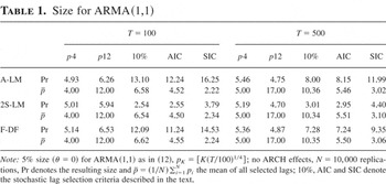
We present results for two different sample sizes: T = 100 and T = 500; further results for T = 200 and T = 1,000 are available upon request. No constant is included in the test regressions, and d = 1. Only two-sided tests were computed at the nominal level of 5%. We simulate with θ = 0 to explore size properties. Different lag length selection algorithms are employed to approximate the AR(∞) processes by autoregressions of order p: Schwert's deterministic rules with K = 12 and K = 4 (see (8)), sequential testing (see, e.g., Ng and Perron, 1995), and also information criteria, in particular the information criteria by Akaike (AIC) and Schwarz (SIC). Sequential testing was carried out by individual t-tests on the last lag at 10% significance level, where Schwert's rule with K = 12 was also applied to set the maximal lag for sequential testing and information criteria. Table 1 contains rejection frequencies and also means of the selected lag length over N = 10,000 replications. All tests rely on standard t-statistics without heteroskedasticity consistent standard errors.
Size for ARMA(1,1)

All three tests perform similarly well in terms of size if the lag length is selected deterministically following Schwert's rule with K = 4 and K = 12 (the choice of only p2 lags yields experimental size distortions not reported here). For small samples (T = 100), p12 is dominated by p4 in Table 1. But then we observe a result that is rather surprising at first glance: none of the three data-driven lag length selection methods does really work! The A-LM and F-DF tests are always oversized, and the 2S-LM test is undersized in all cases where lag length is estimated from the data, even in large samples (it is worth noting that there are no differences in the means of selected numbers of lags between the tests). At first sight this seems to be counterintuitive, especially if we think about the successful use of information criteria and significance testing applying the ADF test. But in contrast to the ADF test, only (asymptotically) stationary variables are included in the A-LM, F-DF, and 2S-LM test regressions. In particular,

is square summable and therefore stationary as t → ∞. Hence, the test statistics tφ and tai, i = 1,…, p, from regression (6) exhibit a certain amount of stochastic dependence even asymptotically, so that the selected lag length

and the test statistic tφ are dependent random variables. Our simulation evidence is related to the results of Leeb and Pötscher (2005), where the potentially disastrous impact of data-driven model selection on subsequent inference is explored.
This problem is not restricted to the regression-based tests investigated here. The same problem affects the tests of Tanaka (1999) and Robinson (1994). To illustrate this, we simulate xt = εt as a normal i.i.d. series, and we test at the 10% level whether a fitted AR(1) parameter is significant or not. Tanaka's test is then performed with an AR(0) specification, with an AR(1) specification, and with the specification indicated by the outcome of the significance test. Although both the AR(0) and AR(1) specifications produce sizes close to the 5% nominal level, the variant choosing between AR(0) and AR(1) does not work. In the latter case, Tanaka's test is just as conservative (even for T = 1,000) as the 2S-LM test in Table 1. Actually, this result is not surprising, because both tests are asymptotically equivalent. Similar results are available for Robinson's test.
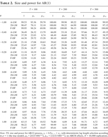
In Table 2 we turn our attention to power for the special case of an AR(1) process and in particular to the question of how much power is lost by implementing some deterministic rule pK given that the true lag length is p = 1. The following features are observed: First, all tests are more powerful when θ < 0 compared to θ > 0. Second, and not surprisingly, the augmentation with the true lag length p = 1 dominates the rule p4, which outperforms p12. In practice, however, the true lag length is not known. Given the superiority of the rule p4 over p12, we, third, rank the tests for p4: A-LM and (optimal) F-DF have very similar empirical (size and) power functions. F-DF is slightly superior for θ < 0, which is no longer the case for θ > 0. Generally, both tests dominate 2S-LM whenever p4 is applied. The power functions are not only asymmetric but also nonmonotonic for θ > 0. In particular, power collapses for θ = 1, unless p = 1 is employed. The reason for that is that this alternative is not fractional but purely autoregressive and hence not detected by the test. The dynamics are rather fully captured by the autoregression so that power is reduced to size. Further Monte Carlo results were collected but are not reported here. In particular, we observed more power for AR(1) processes with negative serial correlation, and we found that Schwert's p4 rule is recommendable also with the more persistent linear process

.
Size and power for AR(1)

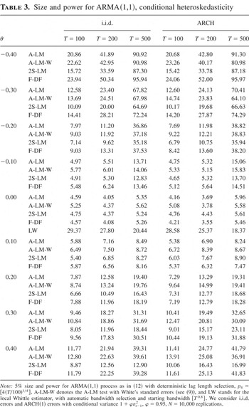
Given the superior performance of p4 over p12 with respect to size and power, we apply p4 to determine the lag length in what follows. Two further tests are now included. The first one builds on a semiparametric estimator of d that is asymptotically normally distributed. In particular, the local Whittle (LW) estimator is investigated because Robinson (1995) shows that it is more efficient than competing semiparametric estimators. Moreover, it has a couple of nice properties: It is robust to conditional heteroskedasticity (see Robinson and Henry, 1999), it remains consistent up to d < 1 and asymptotically normal up to d < 0.75 (Velasco, 1999), and a procedure to compute the required bandwidth m optimally from the data may follow Henry (2001). The second test is the A-LM variant with White standard errors from (9), (A-LM-W). One further aspect of Table 3 is conditional heteroskedasticity. In addition to i.i.d. sequences we allow for ARCH(1) innovations that are close to nonstationarity with conditional variance given as 1 + 0.95εt−12.
Size and power for ARMA(1,1), conditional heteroskedasticity

The LW estimator (or test) is included only under the null hypothesis, and it is computed from the differences of the series, which are I(0). Gross size distortions are observed still for T = 500, and hence the test is not investigated under the alternative. Given i.i.d. innovations we observe for A-LM (and A-LM-W), 2S-LM, and F-DF similar results as in Table 2: Tests against θ < 0 are more powerful than against θ > 0; A-LM, A-LM-W, and F-DF display very similar power functions and dominate 2S-LM. Under the assumption of the rather persistent ARCH(1) volatility we find that the White corrected version A-LM-W is closest to the nominal level, although the other tests (except for LW) work remarkably well under the null. At the same time A-LM-W is most powerful as long as |θ| ≤ 0.2. We conclude that use of White standard errors seems to be a good strategy given the fact that they have no negative affect with i.i.d. innovations and they improve the test under ARCH errors.
5. SUMMARY
Several variants of the LM test for integration against fractional alternatives have been studied since Robinson (1991). An open challenge still is how to account for serial short-run correlation as opposed to long memory and how to correct for heteroskedasticity. Those aspects are tackled in the present paper, where we present a lag augmented LM test, which is completely regression based and recommended with White's standard errors.
Our findings are the following. Lag augmentation leaves the limiting normal distribution unchanged. The short memory component does not have to be an ARMA process; it may follow a general linear process with weaker summability conditions. The limiting distribution is retained as long as the number of lags is growing with the sample size at appropriate rate. Further, the innovations driving this process are not required to be serially independent. We rather consider an MDS allowing for conditional heteroskedasticity. Finally, the new test is compared with competing procedures in Monte Carlo experiments. Special focus is on different strategies for model selection accounting for serial short-run correlation. It turns out that data-dependent rules for lag length selection do not provide valid inference for any of the tests, which is in line with findings by Leeb and Pötscher (2005). Therefore, we propose a simple deterministic rule of thumb. Moreover, the investigated correction for heteroskedasticity seems to improve the behavior in the presence of ARCH.
We only considered regression-based tests because we are not aware of empirical strategies regarding how to fit a model to the short-run component otherwise. For empirical work our findings may be cast into the following guidelines. (i) The number of lagged differences should not be determined following information criteria or significance of their coefficients. Such a stochastic, data-driven model selection (which is usually employed with the ADF test) implies invalid inference. (ii) Therefore, we explored deterministic choices of lag length selection, in particular pK = [K(T/100)1/4] for a sample of length T. For a variety of samples sizes and simulated processes we observed that K = 4 is large enough to yield experimental sizes of the tests close to the nominal one under the null hypothesis. At the same time, the power is reduced under the alternative as pK grows for given T. Therefore, we recommend working with p4 = [4(T/100)1/4] in practice and eventually varying the lag length around this value to check whether test results are robust and hence reliable with respect to the number of lags. (iii) Our proposed lag augmented LM (A-LM) test performed in one step is in finite samples superior to the two-step variant proposed by Breitung and Hassler (2002). (iv) We investigated the F-DF test by Dolado et al. (2002), too. It depends on a parameter d* that one has to choose. Throughout, we simulated with the optimal choice following Lobato and Velasco (2005). This variant behaves very similarly to our new test and is mildly more powerful under some alternatives. In practice, however, the optimal choice is not known but has to be estimated. The effect of uncertainty due to estimating d* on the F-DF test has not been addressed. (v) The power function is asymmetric. The tests are clearly more powerful when testing against d < d0 than under alternatives d > d0. In particular, under the alternative d0 + 1 power reduces to size because the alternative is not fractional but purely autoregressive and hence is not detected when lags are included. (vi) Monte Carlo experiments suggest that the considered tests are fairly robust with respect to some conditional heteroskedasticity. Nevertheless, we observe that our proposal to compute the A-LM test with White standard errors may improve the performance. At the same time, the correction for heteroskedasticity does no harm when no heteroskedasticity is present.
APPENDIX
Throughout the Appendix, we use for matrices the matrix norm induced by the euclidean vector norm, defined for any m × n matrix A as

. Further,

denotes the sequence of autocovariances of any stationary process ut, and

denotes the sequence of cross-covariances of ut with vt (also stationary). Explicitly, γj*x denotes cross-covariances of xt** (defined in (A.1), which follows, and xt. Finally, all sums are over {p + 1,…,T}, unless stated otherwise.
A.1. Auxiliary Lemmas.
LEMMA 1. Let Assumptions 1 and 2 hold true and define the process xt−1**

It then follows that the process xt−1** is square summable,

.
Proof of Lemma 1. The proof is omitted and provided in the working paper version instead. █
LEMMA 2. Consider the regression equation (6) and its ordinary least squares (OLS) estimator

but use the stationary process xt−1** instead of xt−1* and denote the corresponding OLS estimator as

. Then it follows that
(i)

, and
(ii)

.
Proof of Lemma 2. Define Δt−1* = xt−1** − xt−1*. It holds that

with

. Holding t fixed and letting j → ∞, it follows immediately that

Thanks to the MDS property of εt, we can write

or, equivalently,

.
The proof is completed along the lines of the proof of Proposition 4, which appears later in this Appendix; a complete argumentation is provided in the working paper version. █
LEMMA 3. For absolutely summable sequences {dj}j≥0, it holds that dj = o(j−1). For one summable sequences, it holds that dj = o(j−2). Finally, for absolutely summable multidimensional sequences,

, it holds that |di1… ik| = o(|i1|−1·····|ik|−1).
Proof of Lemma 3. Assume that dj = O(j−1) or has an even lower convergence rate. Then, [sum ]j≥0 dj diverges, and so {dj}j≥0 must be o(j−1). The proof proceeds similarly for one summable and multidimensional sequences. █
LEMMA 4. The cross-covariances

and the autocovariances

are square summable,

, and

.
Proof of Lemma 4. It holds that

Because of the MDS property of εt, only terms for which t − h − i = t − 1 − j have nonzero expected value, and so

Further, bi = o(i−1) because of Lemma 3 and ψi+h = O((i + h)−1); see the proof of Lemma 1 in the working paper version. Then,

With

it follows that

which leads to the desired result. The proof runs similarly for the autocovariance sequence γh*. █
LEMMA 5. Consider the vector Wtp = (xt−1**,xt−1,…, xt−p)′ and define the variance-covariance matrix

. Then, Σp is nonsingular and ∥Σp∥ and ∥Σp−1∥ are bounded as p → ∞.
Proof of Lemma 5. Note that Σp is singular if and only if the components of Wtp are linearly dependent, which is not the case. Then, we may obviously write

where Σ*p = (γ0*x,…, γp−1*x)′ and Σxp is the p × p autocovariance matrix of xt. Then, by triangle inequality, we obtain

From the definition of the norm it follows that the norm of a matrix B obtained by bordering a matrix A with zeros equals the norm of A, and so

The euclidean norm of Σ*p converges to a constant as p → ∞ because of square summability of γh*x, whereas the norm ∥Σxp∥ is bounded (Berk, 1974, p. 493).
The inverse can be computed (Lütkepohl, 1996, p. 148) from

with


Then,

and the desired result follows from


because ∥Σxp−1∥ < ∞ (Berk, 1974, p. 493), and σωp2 (defined in Lemma 6, which follows) converges to a positive constant. █
LEMMA 6. The sequence σωp2 = γ0* − Σ*p′Σxp−1Σ*p converges to a positive constant as p → ∞.
Proof of Lemma 6. Begin by expressing σωp2 as a series. To this end, one can use the decomposition

given in Berk (1974, p. 491) with

where, for given j ∈ {1,…, p},

represent the solutions to the minimum problem

or, equivalently, the values of the OLS estimators


are consistent for the conditions T → ∞ and j fixed. Because xt is ergodic with finite variance, the necessary conditions for Theorem 4.1.1 from Amemiya (1985), the theorem that ensures the claimed consistency, can be shown to be met. The matrix Dp has diagonal structure

where

is the respective minimum,

Obviously,

and

as p → ∞. Then,

and

It follows that

Note that σωp2 is bounded, |σωp2| ≤ |γ0*| + ∥Σ*p′∥∥Σxp−1∥∥Σ*p∥ < ∞. Hence, a sufficient condition for convergence in (A.2) is

as p → ∞. Because

converges to a nonzero constant, the sequence

is bounded, and this condition reduces to

. Standard OLS algebra leads to

with Xtp = (xt−1,xt−2,…, xt−p)′. Because xt is ergodic, it holds that

and

For any i,

or

The norm of Σxj−1 is bounded, and so

. Because

and ai = o(i−2) = o(i−1) we have

and also

and so it holds that

, as needed for the convergence result. Because it is the diagonal element of a positive definite matrix, Σp−1, the limit of σωp2 must be positive. █
LEMMA 7. The process utp = Σ*p′Σxp−1 Xtp, with Xtp = (xt−1,xt−2,…, xt−p)′, converges in probability as p → ∞ to a square summable process,

.
Proof of Lemma 7. Represent Xtp as a countable linear combination of the MDS innovations εt−1−j, j ≥ 0:

where Bp and εt−1 have infinitely many columns and lines respectively:


Note that, because the sequence {bj}j≥0 is s-summable, the norm of Bp is bounded as p → ∞. Then the process utp is nothing more than a linear process with innovations εt−1−j, j ≥ 0:

with coefficients that can be obtained by calculating the multiplication Σ*p′Σxp−1Bp. This is just another way of expressing the convolution of the filters Σ*p′Σxp−1, which is an MA(p), and {bj}, which is MA(∞). Denote by ut the asymptotic counterpart of utp,

where the coefficients ζj are obtained as a limit of the convolution Σ*p′Σxp−1Bp for p → ∞. The coefficients ζj are square summable, because

the matrices having bounded norms as p → ∞ (see Lemma 5 and the properties of Bp). Consider now the difference of the processes given by (A.3) and (A.4):

with second moment

From the definition of ut, it follows that

This leads to

as p → ∞, from which the result follows. █
LEMMA 8. Assume the fourth-order cumulants of the innovations εt are absolutely summable in the sense that

Then, the fourth-order cumulants of a linear process yt, yt = [sum ]j≥0 ψjεt−j, with ψ0 = 1 and |ψj| = O(1/(j + 1)) (a) are finite, and (b) satisfy the following summability condition:

Proof of Lemma 8. The proof is omitted and provided in the working paper version instead. █
LEMMA 9. The expression

is bounded for all p.
Proof of Lemma 9. Gonçalves and Kilian (2003) show that

is bounded for all p, and we use the same arguments here. Consider

and denote bj,p = (bj−1,…, bj−p)′ so that

and

where

for i ≠ j and

for i = j. We can also write

, and we obtain

Here ∥Σ*p∥ is bounded by Lemma 4 and ∥bj,pψi∥ is bounded because of the absolute summability of xt, and finally the assumption of absolutely summable eighth-order cumulants leads to the desired result. █
LEMMA 10. The sum

is bounded.
Proof of Lemma 10. The proof is omitted and provided in the working paper version instead. █
A.2. Propositions.
Proof of Proposition 1. From Lemma 2 we know that there is no difference between the variable xt−1* and its stationary counterpart xt−1** asymptotically, and so we may assume xt−1** to be observable and investigate the consistency of the corresponding OLS estimator. Let Wtp = (xt−1**,xt−1,…, xt−p). We get the OLS estimator as follows:

and accordingly

where

. Denote

and Σp the corresponding covariance matrix, where

,

, and

so that

Recall that ∥Σp∥, ∥Σp−1∥ are bounded because of Lemma 5. We assume that p = o(T1/4), or p4/T → 0, and adopt Lemma 3 from Berk (1974, p. 493) and auxiliary Lemma A.2 from Gonçalves and Kilian (2003, p. 14) in our case to show that

By the use of the spectral matrix norm we know that ∥A∥2 ≤ [sum ]i,j ai,j2 for any real matrix A = ai,j. The convergence of all elements included in Σxp, given the absolute summability of the process xt, is proved in Berk (1974) for the i.i.d. case and in Gonçalves and Kilian (2003, Lem. A.2) under the MDS assumption for εt. Therefore, we only are concerned about the components γ0* and Σ*p, which are generated by the square (but not absolutely) summable process xt**. We consider

which according to Gonçalves and Kilian (2003, Lem. A.2) is bounded by

where κ*(l1,l2,l3,l4) and γ0* denote the fourth-order cumulants of xt** and its autocovariances, respectively. The first sum is bounded (see Lemma 8), just like the second one, because of square summability of the autocovariances of xt** (see Lemma 4). Analogous results in the case of Σ*p can be shown in a similar way. Because of (A.7), we now have

where C is some positive constant. Then

because p4/T → 0 by assumption. The desired result follows now by

This result is used to prove consistency of the parameter estimates as follows:


Obviously

. To guarantee

-consistency we assume that

Equation (A.10) also determines our summability condition from Assumption 2, because as we know from Brillinger (1975, p. 52)

implies

. Thus, p must be of order higher than O(T1/2s) to allow for (A.10), and we need s > 2 in Assumption 2 to hold the upper bound p = o(T1/4). The results in Gonçalves and Kilian (2003, Thm. 2.1) and (A.10) lead without any considerable modification to

Now consider (A.9). We have


where (A.13) is O(pT−1) by Gonçalves and Kilian (2003, Thm. 2.1), and we only need to examine (A.12):

where

which is bounded by the absolute summability of eighth-order cumulants of εt and Lemma 10. The following result is now obvious:

By combining (A.11) and (A.14), we have

Now it is easy to see that

and therefore also

. █
Proof of Proposition 2. Define Xtp = (xt−1,…, xt−p)′ so that Wtp = (xt−1*,Xtp′)′. Now we have

where βp = (0,a1,…, ap)′. We investigate the asymptotic distribution of

, but from Lemma 2 we know that the difference to

vanishes asymptotically, and so we only have to study the asymptotic distribution of the latter term. Now we find an expression for

as follows:

where

We can also denote the estimated values of the true matrices in a more compact way:

Further, we define the asymptotic counterpart of

as follows:

Now we need to show that

To prove (A.15), denote

and A = [γ0* − Σ*p′Σxp−1Σ*p]−1 = σωp−2. We have

and we will show that this expression converges in probability to zero. Consider the first term following the equals and conclude according to (A.11) that

and

because of (A.5). Furthermore, it is easy to see that |T−1/2 [sum ]xt−1**εt| = Op(1) and

. The desired result is now obvious:

Denote

and B = [γ0* − Σ*p′Σxp−1Σ*p]−1Σ*p′Σxp−1 = AΣ*p′Σxp−1. Then we have

Consider the last term. We proceed with the following transformation:

where utp = Σ*p′Σxp−1 Xtp and

is bounded, because, according to Lemma 6, it converges to a constant as p grows. From Lemma 7, we know that utp = ut + op(1), where ut is a square summable process with the same innovations εt. It follows that

and similarly to (A.16) we conclude that

It is rather tedious but straightforward to show that

, and so the following relationship holds:

For the remaining term, it holds that

because of (A.11). Statement (A.15) is now proved.
Having shown that the distribution of

can be studied employing an expression with the same asymptotic distribution, we now investigate the distribution of this expression. We have

Denote πp2 as the variance of the term in the sum and calculate it:

Now we can define the following process with zero mean and unit variance:

Because the third term was shown in Gonçalves and Kilian (2003) to converge, it follows with Lemma 9 that πp2 is bounded and converges to a positive constant as T → ∞. We have to prove that

To that end, we apply a central limit theorem (CLT) for martingale differences (cf. Davidson, 1994, p. 383). Hence we need to show that
(a)

and
(b)

.
We start with (a) and have

where S1T, S2T, S3T are defined implicitly and are examined next. Consider

Because p = o(T), we may write

Because of stationarity, we employ a change of variable, τ = s − t, and have the following transformation neglecting the o(1) term:

Employing Theorem 2.3.2 of Brillinger (1975, p. 21) we can express the covariances in the last equality as the sum of products of cumulants of εt of order eight or lower; see also Gonçalves and Kilian (2003). We only consider the component of the sum including eighth-order cumulants. Lemma 10 shows that the following sum is finite:

The sums over other indecomposable partitions can be shown to be finite in the same way. This result implies that ∃K > 0, so that

Next we consider the second term,

where

We have

which equals

bounded by

again considering that p = o(T). The proof of boundedness of the covariance sum is similar to the case of S1T, and we have

because of p4/T → 0. The convergence of S3T is proved in Gonçalves and Kilian (2003), so that

which proves (a), given that πp−2 and ∥Σ*p′Σxp−1∥ are bounded; see Lemmas 9 and 5.
To prove (b) we note that for any η > 0 and some r > 1

By the Cauchy–Schwarz inequality we have

where πp−1 = O(1) and

for all r ≤ 4 by our assumptions. Now consider

where

and further

for all r ≤ 4 by the assumption about cumulants of εt and Lemma 8, which can be easily extended to the case of eighth-order cumulants of xt given the summability of eighth-order cumulants of εt, and also ∥Σ*p′Σxp−1∥ < ∞ according to Lemma 5. Finally,

because

for some r ≤ 4 and i = 1,…, p, and therefore we have

, leading to

for r = 3 because of p4/T → 0. The proof of (A.17) is now complete.
Now we define the matrix

where it is easy to see that

Obviously, (A.17) can be represented as

However, in practical applications Γp is of course unknown and therefore needs to be estimated consistently. We proceed in the manner of Gonçalves and Kilian (2003, Thm. 2.3) and estimate the matrix of fourth moments in the following way:

which is a version of the Eicker–White heteroskedasticity-robust estimator, where Vtp = (xt−1*,Xtp′)′ and

. Using Lemma 2 and Proposition 1 it is easy to show that

and employing the arguments of Theorem 2.3 in Gonçalves and Kilian (2003), results (A.18) and (A.19), and the assumption p4/T → 0 (for reference, see Gonçalves and Kilian, 2003, proof of Thm. 2.3), we conclude that

in (A.20) is a consistent estimator of the matrix of fourth moments. It also follows with slight modifications that

, with

defined in (9), has a proper positive probability limit as T → ∞. The desired result now follows. █
Proof of Proposition 3. Consider the OLS estimator under the local alternative,

. Correspondingly, denote

. Therefore, we have

Let us consider the properties of the process xt−2δ defined in (11). Just as in Lemma 2, define the asymptotic counterpart

in the proof of Lemma 2 and express it as an infinite moving average (MA) process,

, with ηj the convolution of ψj and 1/j. Tedious but straightforward calculations lead to the conclusion ηj = O(ln j/j), which ensures stationarity and ergodicity of the process xt−2δδ. The difference of the processes xt−2δ and xt−2δδ itself has an MA representation,

where the coefficients

, similarly to

in Lemma 2, converge for fixed t and j → ∞ to the theoretical coefficients ηj−1, and so, following Lemma 4, we may write

which, together with the MDS property of εt, leads to

Using the integral ∫(ln2 x/x2)dx = −(ln2 x/x) − (2 ln x/x) − (2/x) to approximate the sum, it follows that

It is straightforward to show, along the lines of Proposition 4, that

and so

“converges” to Σp. Now, consider the expression

. It can be easily seen that

where

Write

with

, or

Consider the first element of this vector:

Let

, with

, and note that

as p → ∞. Then, write

, with

. Postmultiply Bp with Σxp to obtain

We now have

where Σxp[j] is the jth column of the matrix Σxp. Further,

It follows that

and hence

Because the norms of the matrix Σxp and the vector

are bounded, it follows that the norm of Ap vanishes as p → ∞, and, because of the convergence of γ0* − Σ*p′Σxp−1Σ*p and of Qp, it holds that

It follows directly from the distribution of the estimators that

is of order op(p−1/2), and, because of this consistency, it is straightforward to show that the standard deviation of

behaves just as under the null hypothesis, which completes the result. █
Proof of Proposition 4. The proof consists of three steps. First, we show

.
To this end, recall that di = O(i−d−1) and d0 = 1. Then,

Now write

For t → ∞, it obviously holds that

, which is finite as long as α > −1 and d > 0. Thus the sum on the right-hand side of equation (A.22) is bounded and

OLS regression of xt,obs on (1 − L)td f (t) leads to

Two cases arise. On the one hand, α − d ≥ 0. Then, write

and the following result is easily shown to hold with W a Brownian motion:

It follows that

and, because (t/T)α−d = O(1),

On the other hand, α − d < 0, where we distinguish three subcases: −0.5 < α − d < 0, α − d = −0.5, and α − d < −0.5. For −0.5 < α − d < 0, we obtain just as before

from which it follows that

because T−0.5−(α−d)tα−d = T−0.5−(α−d)t0.5+α−dt−0.5 and (T/t)−0.5−(α−d) = O(1). For α − d = −0.5, the denominator of

is obviously O(ln T). With

, the variance of the numerator is

Because of Lemma 3, γj−ix = o((j − i)−1). Then,

The first summand on the right-hand side dominates the second, and, because j ≤ T, we obtain

Hence, because T > T − i,

The numerator is thus of order

, and

, leading to

For α − d < −0.5, the denominator of

converges to a constant. The numerator can be shown to be Op(1), and so

Note that the Op(t−0.5) terms in equations (A.23)–(A.26) can be written as O(t−0.5)·Op(1), where the Op(1) term is the same for all t.
In the second step, the term

is examined:

Further,

Because

,

,

, and, from Lemma 2, xt−1* = xt−1** + Op(t−0.5), it follows that

Again, the stochastic component of this

term is the same for all t.
The third step is concerned with the effect of these approximations on the estimators. Let

and consider

and

, thus accounting for equations (A.23)–(A.26) and also for (A.27). The OLS estimator

of βp is given by

First, we need to show that

and

Because inverting a matrix and building a matrix norm are continuous operations, the matrix (1/T)[sum ]WtpWtp′ is nonsingular with probability one for any fixed p; see Lemma 5. Consider the first diagonal element of

, which can be expressed as

because of [sum ](ln2 t/t) = O(ln3 T) and

Similar arguments apply to the other elements of

and

, which leads to

Hence,

because of

. Also,

Because

and ∥1p+1∥ are both of (stochastic) order

, it is easily derived that

Then we need to show that

where

. Elementary manipulations (the complete argumentation can be found in the working paper version) of

lead to the following expression for

:


For each term, the norm of

is bounded, and so is the norm of βp. The expression (A.29) is of stochastic order

Although

, the second term is trickier. Consider

. Because

for any λ > 0, we may choose some λ ∈ (0,0.25) and write

But

which is Op(1), because its variance,

, is easily checked to be finite. Hence,

is op(Tλ), as is

, in spite of long-range dependence of xt−h**. Because

, we have

, and, obviously, so is the expression (A.30). Finally, (A.28) can be shown to be op(1) using equation (7) and similar reasoning as before, thus concluding the proof. █