1 Introduction
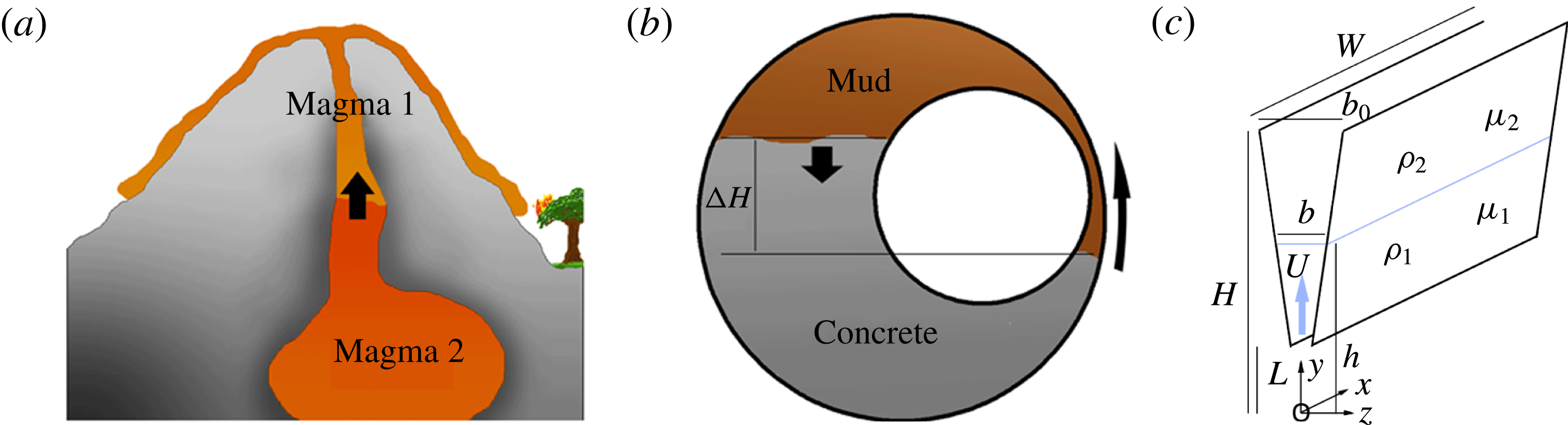
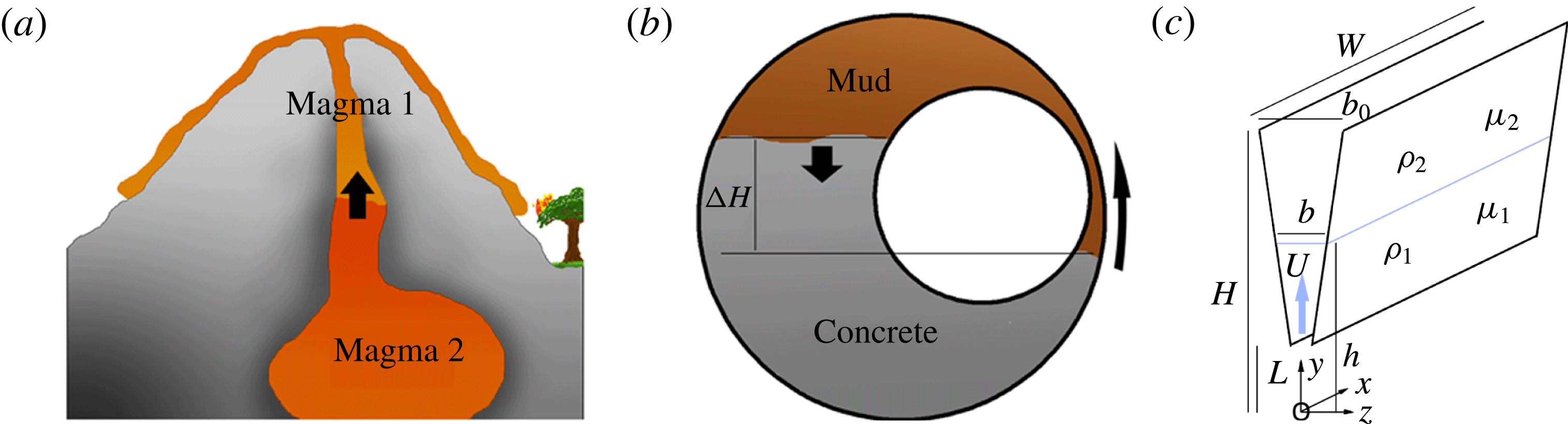
There are several situations in which fluid is squeezed through a narrow channel of variable width displacing a second fluid of different density or viscosity. For example, magma rising along a dyke from a stratified subsurface reservoir to the Earth’s surface may displace magma which issued earlier in the eruption sequence (Blake & Ivey Reference Blake and Ivey1986; figure 1 a), and cement which is pumped between a well bore and the casing pipe will displace the drilling mud and prevent fluid leakage from the exterior of an oil well. In this latter situation, the annular channel is often asymmetric, leading to channelling of the flow along the wider part of the annulus, and formation of an extensive along-annulus interface. Subsequently, a net hydrostatic pressure gradient may displace this interface in the azimuthal direction (figure 1 b). In coating flows, where a roller is used to apply a thin layer of fluid to a flat surface, the geometry of the roller forces a flow through a channel of variable width, leading to a flow with similar geometric constraints (see e.g. figure 8 of Ruschak (Reference Ruschak1985)).
(a) Illustration of a volcano in which magma of one composition is being forced up a dyke by magma of another composition. (b) Illustration of flow in a well bore, where, owing to the initial injection of the concrete along the well, the interface between the concrete and less dense mud has a different height on each side of the central pipe. This leads to a buoyancy-driven net azimuthal flow. (c) A schematic of the model flow geometry, with
 $W$
the along-channel length,
 $L$
the height of the inflow to the channel above the origin,
 $H$
the height of the outflow above the origin,
 $b_{0}$
the channel width at the outflow,
 $h$
the height of the interface above the origin and
 $b$
the width of the channel at the interface
 $h$
where mean upflow speed is
 $U$
.
With such fluid–fluid interfaces migrating through a narrow channel, instabilities may arise. First, owing to the viscosity difference between two fluids, if the less viscous fluid displaces the more viscous fluid, a Saffman–Taylor (ST) instability may develop (Saffman & Taylor Reference Saffman and Taylor1958; Homsy Reference Homsy1987). Second, if the more dense fluid is initially above the less dense fluid, a Rayleigh–Taylor (RT) instability may form (Gertsenshtein et al.
Reference Gertsenshtein, Kozlov, Prokof’ev, Reznichenko, Chernyi and Chernyavskii2008). Third, the surface tension in a direction transverse to the flow and parallel to the cell walls (we will refer to this as the perturbation surface tension) has a stabilising influence especially on short-wavelength perturbations to the interface. Fourth, the convergence of the channel causes a geometric instability, due to the quasi-static acceleration of the fluid as it is forced into the narrower part of the cell. This instability becomes dominant when the wavenumber
 $k$
is small.
There have been many analyses of these instabilities, as summarised in the seminal review by Homsy (Reference Homsy1987), in which both the linear and the nonlinear growth of the instability are discussed. Numerous studies have examined the effects of various complexities, including surface roughness (Chen Reference Chen1987; Paterson et al. Reference Paterson, Fermigier, Jenffer and Limat1995), temperature-dependent rheology relevant to lavas (Bruce & Huppert Reference Bruce and Huppert1989) and non-Newtonian fluids (Fontana, Dias & Miranda Reference Fontana, Dias and Miranda2014). Recently there has been interest in the problem of techniques to control the stability of the interface, by variation in flow rate (Dias, Parisio & Miranda Reference Dias, Parisio and Miranda2010; Brandao, Fontana & Miranda Reference Brandao, Fontana and Miranda2014), cell width (Zheng, Kim & Stone Reference Zheng, Kim and Stone2015), geometry (Brandao et al. Reference Brandao, Fontana and Miranda2014) and the effect of gap thickness (Al-Housseiny, Tsai & Stone Reference Al-Housseiny, Tsai and Stone2012; Al-Housseiny & Stone Reference Al-Housseiny and Stone2013; Dias & Miranda Reference Dias and Miranda2013).
The effect of a variable gap width is analogous to the original discovery of Pearson (Reference Pearson1960) and Pitts & Greiller (Reference Pitts and Greiller1961) in their analysis of the ribbing instability which is produced when a film of paint emerges from a roller moving across a plane. In that case, the air–paint interface is fixed relative to the roller, and the gradient in capillary pressure associated with perturbations to the position of this interface leads to stability of the interface, which otherwise becomes unstable by a process analogous to the ST instability. In that application the instability leads to formation of ribs in the emerging flow. More recently, the phenomenon by which a gradient in capillary pressure stabilises an interface was recognised formally in the context of ST instability by Al-Housseiny et al. (Reference Al-Housseiny, Tsai and Stone2012). They examined the case in which an interface moves at a constant speed through a tapering cell and found a condition for stability of the interface.
However, in considering flow through a tapering channel of finite size, the boundary conditions have an important influence on the speed of the interface as a function of the position within the channel. In turn, this has an impact on the stability of the interface. We focus on the case of a constant volume flux through the channel, but we also show that qualitatively similar results apply if there is a constant pressure difference applied across the channel. We show that, in both cases, the stability of the interface evolves as it migrates through the channel. These effects may be understood by considering the local pressure gradients within the channel.
For a fixed volume flux
 $Q$
in a tapering channel, conservation of mass implies that the flow speed changes with position along the cell. For a cross-channel average velocity
 $v$
and local channel width
 $b$
,
 $v\sim Q/b$
. This flow is resisted by the effect of no slip on the walls, giving an along-channel pressure gradient
 $$\begin{eqnarray}\frac{\text{d}p}{\text{d}y}=-12\unicode[STIX]{x1D707}\frac{Q}{b^{3}},\end{eqnarray}$$
where
 $y$
is the coordinate in the direction of flow. The change in pressure gradient across the interface from fluid of one viscosity to fluid of a second viscosity drives the ST instability, and from (1.1) we anticipate that this effect increases in magnitude at a rate proportional to
 $1/b^{3}$
as
 $b\rightarrow 0$
.
The pressure jump across the interface associated with surface tension is due to the narrow channel width (we will refer to this as the in-channel surface tension)
 $\unicode[STIX]{x0394}p=(2\unicode[STIX]{x1D6FE}\cos \unicode[STIX]{x1D703})/b$
, where
 $\unicode[STIX]{x1D703}$
is the contact angle and
 $\unicode[STIX]{x1D6FE}$
is the surface tension. In writing this expression, we have neglected the thickness of a residual wetting layer and the correction terms to the pressure jump: this is valid for small capillary number
 $Ca$
and a small channel width, as calculated by Park & Homsy (Reference Park and Homsy1984) and numerically demonstrated by De Lozar, Juel & Hazel (Reference De Lozar, Juel and Hazel2010). In this limit, the gradient of this pressure jump in the direction of flow,
 $y$
, increases at a rate proportional to
 $1/b^{2}$
, as given by the relation
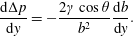 $$\begin{eqnarray}\frac{\text{d}\unicode[STIX]{x0394}p}{\text{d}y}=-\frac{2\unicode[STIX]{x1D6FE}\cos \unicode[STIX]{x1D703}}{b^{2}}\frac{\text{d}b}{\text{d}y}.\end{eqnarray}$$
Comparing (1.1) and (1.2), we find that, with an adverse viscosity ratio, the ST instability is able to develop in the narrowest part of the cell, while further upstream in the wider part of the cell, the gradient in capillary pressure due to in-channel surface tension is able to suppress the viscous instability. A qualitatively similar result applies with a constant pressure jump across the cell, although in this case, as the ratio of the volume of the less viscous to the more viscous fluid in the channel changes, there is a gradual change in flux, leading to a difference in detail in stability behaviour (§ 4).
In contrast, Al-Housseiny et al. (Reference Al-Housseiny, Tsai and Stone2012) and Al-Housseiny & Stone (Reference Al-Housseiny and Stone2013) considered the situation in which the interface speed is constant, and hence in which the viscous pressure gradient scales as
 $$\begin{eqnarray}\frac{\bar{u}\unicode[STIX]{x1D707}}{b^{2}}\end{eqnarray}$$
while the pressure gradient associated with the ST instability scales as
 $$\begin{eqnarray}\frac{\unicode[STIX]{x1D6FE}}{b^{2}}\frac{\text{d}b}{\text{d}y}.\end{eqnarray}$$
In this case, with
 $\text{d}b/\text{d}y$
being constant, the issue of stability is independent of position in the channel, and hence the result of Al-Housseiny et al. (Reference Al-Housseiny, Tsai and Stone2012) shows that, to keep the interface at conditions for incipient instability, the supply flux should change exactly in step with the change in channel width at the location of the interface.
We can build on these results by considering the effect of a density difference between the two fluids, which can lead to RT instability if the dense fluid overlies the less dense fluid, as driven by the buoyancy force
 $g\unicode[STIX]{x0394}\unicode[STIX]{x1D70C}$
. In a Hele-Shaw cell of uniform thickness, both the buoyancy-derived pressure gradient (BPG) and the viscous pressure gradient (VPG) are constant, and so the overall stability can be determined by consideration of the difference between the BPG and VPG, such that a stabilising VPG can suppress RT instability and a stabilising BPG can suppress ST instability, as described by Hill (Reference Hill1952) and Phillips (Reference Phillips1991, pp. 163–165). However, in the tapering channel, as described above, the VPG evolves with position, while the BPG is constant. If the geometric instability is suppressed (when fluid flow is directed into the wider section of the channel) and the VPG is stabilising, while the BPG is destabilising, it may now be the case that the system is absolutely unstable in the widest part of the channel, while being absolutely stable in the narrowest part of the channel, in contrast to the classical results of Hill (Reference Hill1952) and Phillips (Reference Phillips1991) for a channel of constant width.
In the different case that both effects are destabilising, the VPG may dominate in the narrowest part of the channel while the BPG may dominate in the widest part. Moreover, in this situation, the stabilisation which may be associated with the gradient in capillary pressure due to in-channel surface tension may in fact lead to a central region of the channel in which the system is stabilised to all effects except for the geometric instability. This region of the channel is bounded by the narrow part of the channel which is unstable to ST instability, and the wider part of the channel which is unstable to RT instability.
We explore the interaction of these effects in detail, developing an analysis of the stability of a moving interface in a channel of finite extent,
 $L<y<H$
, in the direction of flow. Figure 1(c) shows the model geometry, with relevant parameters labelled, including the height of the interface
 $h$
, the height of the top of the tank
 $H$
and the height of the bottom of the tank
 $L$
relative to the point
 $y=0$
defined as the point where the channel width,
 $b$
, would be zero if the channel extended to
 $y=0$
. Since the stability evolves as the interface moves through the channel, we also explore the evolution of the most unstable wavenumber as the interface migrates through the channel.
2 Governing equations
The geometry of the flow is illustrated in figure 1(c). The top of the cell has position
 $y=H$
; the base of the cell is given by
 $y=L$
(if
 $L=0$
then the cell tapers to
 $b=0$
); and the location of the interface is given by
 $y=h(t)$
, where
 $L<h<H$
. The cell is taken to have width
 $W$
in the cross-flow direction,
 $0<x<W$
. The thickness of the cell is given by
 $b=\unicode[STIX]{x1D6FC}y$
, with
 $\unicode[STIX]{x1D6FC}\ll 1$
, and
 $b_{0}=\unicode[STIX]{x1D6FC}H$
:
 $\unicode[STIX]{x1D6FC}$
is the wedge slope. For a flow in the
 $y$
direction with flux
 $Q$
per unit length in the
 $x$
direction, the Reynolds number
 $R=Q/\unicode[STIX]{x1D708}$
. Here we focus on
 $R\ll 1$
, allowing us to use the lubrication approximation (Wooding & Morel-Seytoux Reference Wooding and Morel-Seytoux1976; Dias & Miranda Reference Dias and Miranda2010). The velocity, pressure, viscosity and density in layer
 $i$
are denoted
 $u_{i}$
,
 $p_{i}$
,
 $\unicode[STIX]{x1D707}_{i}$
and
 $\unicode[STIX]{x1D70C}_{i}$
. Momentum and mass conservation then take the form
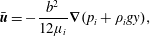 $$\begin{eqnarray}\displaystyle & \displaystyle \bar{\boldsymbol{u}}=-\frac{b^{2}}{12\unicode[STIX]{x1D707}_{i}}\unicode[STIX]{x1D735}(p_{i}+\unicode[STIX]{x1D70C}_{i}gy), & \displaystyle\end{eqnarray}$$
 $$\begin{eqnarray}\displaystyle & \displaystyle \unicode[STIX]{x1D735}\boldsymbol{\cdot }(b\bar{\boldsymbol{u}})=0. & \displaystyle\end{eqnarray}$$
In a converging cell,
 $b=\unicode[STIX]{x1D6FC}y$
, these equations suggest that
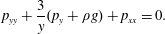 $$\begin{eqnarray}p_{yy}+\frac{3}{y}(p_{y}+\unicode[STIX]{x1D70C}g)+p_{xx}=0.\end{eqnarray}$$
If we consider a flow with vertical volume flux
 $Q$
, the channel-averaged velocity in the
 $y$
direction, at the point
 $y$
, is
 $\bar{v}=Q/\unicode[STIX]{x1D6FC}y$
and the pressure in the
 $i$
th layer is given by
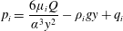 $$\begin{eqnarray}p_{i}=\frac{6\unicode[STIX]{x1D707}_{i}Q}{\unicode[STIX]{x1D6FC}^{3}y^{2}}-\unicode[STIX]{x1D70C}_{i}gy+q_{i}\end{eqnarray}$$
in each fluid layer
 $i$
. For a constant volume flux, the values
 $q_{i}$
are related by the pressure jump due to in-channel surface tension at the boundary. For unidirectional flow, the material boundary condition at the interface
 $y=h$
is
 $$\begin{eqnarray}\frac{\text{d}h}{\text{d}t}=\frac{Q}{\unicode[STIX]{x1D6FC}h}.\end{eqnarray}$$
Hence the evolution of the flat interface is governed by
 $h=\sqrt{(2Q/\unicode[STIX]{x1D6FC})t+h_{0}^{2}}$
, where
 $h_{0}$
is the initial interface height.
For calculation of the interface stability, we now consider a perturbation to the flow of the form
 $$\begin{eqnarray}\displaystyle & \displaystyle p_{i}=\frac{6\unicode[STIX]{x1D707}_{i}Q}{\unicode[STIX]{x1D6FC}^{3}y^{2}}-\unicode[STIX]{x1D70C}_{i}gy+q_{i}+\unicode[STIX]{x1D700}p_{i}^{\prime }(y)\text{e}^{\text{i}kx+\unicode[STIX]{x1D70E}t}, & \displaystyle\end{eqnarray}$$
 $$\begin{eqnarray}\displaystyle & \displaystyle h_{1}=h+\unicode[STIX]{x1D700}\unicode[STIX]{x1D702}_{0}\text{e}^{\text{i}kx+\unicode[STIX]{x1D70E}t}, & \displaystyle\end{eqnarray}$$
where
 $\unicode[STIX]{x1D70E}$
is the growth rate and
 $x$
is the direction transverse to the flow, in the plane of the cell. Substituting these perturbations into (2.1) and (2.2) leads to the equation governing the perturbation to the pressure field:
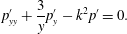 $$\begin{eqnarray}p_{yy}^{\prime }+\frac{3}{y}p_{y}^{\prime }-k^{2}p^{\prime }=0.\end{eqnarray}$$
This has solution
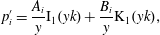 $$\begin{eqnarray}p_{i}^{\prime }=\frac{A_{i}}{y}\text{I}_{1}(yk)+\frac{B_{i}}{y}\text{K}_{1}(yk),\end{eqnarray}$$
where
 $\text{I}_{1}$
and
 $\text{K}_{1}$
are modified Bessel functions of the first and second kind, respectively. The original work of Pearson (Reference Pearson1960) identified some analogous Bessel function-type solutions, and this form of solution was also noted by Al-Housseiny & Stone (Reference Al-Housseiny and Stone2013).
The contact angle
 $\unicode[STIX]{x1D703}^{\prime }$
, measured from the wetting fluid, is the angle the interface makes with the boundary. In a parallel-sided cell, the reciprocal of the radius of curvature of the interface between the two fluids is
 $1/R=(2\cos \unicode[STIX]{x1D703}^{\prime })/b$
. However, if the cell converges, while the contact angle remains the same, the radius of curvature changes at
 $O(\unicode[STIX]{x1D6FC})$
,
 $$\begin{eqnarray}\frac{1}{R}=\frac{2}{b(4+\unicode[STIX]{x1D6FC}^{2})^{1/2}}(2\cos \unicode[STIX]{x1D703}^{\prime }+\unicode[STIX]{x1D6FC}\sin \unicode[STIX]{x1D703}^{\prime })=\frac{2\cos (\unicode[STIX]{x1D703}^{\prime }-\unicode[STIX]{x1D711})}{b},\end{eqnarray}$$
where
 $\tan \unicode[STIX]{x1D711}=\unicode[STIX]{x1D6FC}/2$
. Hence we can redefine an effective contact angle
 $\unicode[STIX]{x1D703}=\unicode[STIX]{x1D703}^{\prime }-\unicode[STIX]{x1D711}$
and use this instead of the true contact angle, to take account of the narrowing of the cell.
For a flow with constant volume flux, we require zero perturbation to the velocity at the top and bottom of the cell. At the interface
 $y=h_{1}+\unicode[STIX]{x1D700}\unicode[STIX]{x1D702}_{0}\text{e}^{\text{i}kx+\unicode[STIX]{x1D70E}t}$
the material boundary condition and pressure jump boundary condition take the forms (Park & Homsy Reference Park and Homsy1984)
 $$\begin{eqnarray}\displaystyle & \displaystyle \frac{\unicode[STIX]{x2202}(\unicode[STIX]{x1D702}_{0}\text{e}^{\text{i}kx+\unicode[STIX]{x1D70E}t})}{\unicode[STIX]{x2202}t}=v_{i}^{\prime }-\frac{Q\unicode[STIX]{x1D702}_{0}\text{e}^{\text{i}kx+\unicode[STIX]{x1D70E}t}}{\unicode[STIX]{x1D6FC}h^{2}}, & \displaystyle\end{eqnarray}$$
 $$\begin{eqnarray}\displaystyle & \displaystyle p_{2}^{\prime }-p_{1}^{\prime }=\unicode[STIX]{x1D702}_{0}\left(\frac{12Q\unicode[STIX]{x1D707}_{2}}{\unicode[STIX]{x1D6FC}^{3}h^{3}}(1-M)+\unicode[STIX]{x0394}\unicode[STIX]{x1D70C}g-\unicode[STIX]{x1D6FE}\left(k^{2}+\frac{2\cos \unicode[STIX]{x1D703}}{\unicode[STIX]{x1D6FC}h^{2}}\right)\right), & \displaystyle\end{eqnarray}$$
where
 $M=\unicode[STIX]{x1D707}_{1}/\unicode[STIX]{x1D707}_{2}$
is the viscosity ratio,
 $\unicode[STIX]{x1D6FE}$
is the surface tension,
 $\unicode[STIX]{x1D703}$
is the contact angle,
 $g$
is the acceleration due to gravity and
 $\unicode[STIX]{x0394}\unicode[STIX]{x1D70C}=\unicode[STIX]{x1D70C}_{2}-\unicode[STIX]{x1D70C}_{1}$
is the density difference. The last term in (2.12) corresponds to the effect of the converging channel.
After some algebra, these boundary conditions lead to a dispersion relation for
 $\unicode[STIX]{x1D70E}$
with a shape function
 $f$
where
 $$\begin{eqnarray}\unicode[STIX]{x1D70E}=\frac{b^{2}k}{12\unicode[STIX]{x1D707}_{2}}\left(\frac{12Q\unicode[STIX]{x1D707}_{2}}{b^{3}}(1-M)+\unicode[STIX]{x0394}\unicode[STIX]{x1D70C}g-\unicode[STIX]{x1D6FE}\left(k^{2}+\frac{2\unicode[STIX]{x1D6FC}\cos \unicode[STIX]{x1D703}}{b^{2}}\right)\right)f(hk,Lk,Hk,M)-\frac{Q\unicode[STIX]{x1D6FC}}{b^{2}},\end{eqnarray}$$
 $$\begin{eqnarray}\displaystyle f=\frac{(c_{2}-\unicode[STIX]{x1D70F}c_{1})(c_{1}-\unicode[STIX]{x1D714}c_{2})}{2kh((c_{1}-\unicode[STIX]{x1D714}c_{2})(\unicode[STIX]{x1D70F}\text{I}_{1}+\text{K}_{1})-M(\text{I}_{1}+\unicode[STIX]{x1D714}\text{K}_{1})(\unicode[STIX]{x1D70F}c_{1}-c_{2}))}, & & \displaystyle\end{eqnarray}$$
where the Bessel functions are evaluated at
 $kh$
and
 $$\begin{eqnarray}\displaystyle & \displaystyle c_{1}=hk(\text{I}_{0}(hk)+\text{I}_{2}(hk))-2\text{I}_{1}(hk), & \displaystyle\end{eqnarray}$$
 $$\begin{eqnarray}\displaystyle & \displaystyle c_{2}=hk(\text{K}_{0}(hk)+\text{K}_{2}(hk))+2\text{K}_{1}(hk), & \displaystyle\end{eqnarray}$$
 $$\begin{eqnarray}\displaystyle & \displaystyle \unicode[STIX]{x1D70F}=\frac{Hk(\text{K}_{0}(Hk)+\text{K}_{2}(Hk))+2\text{K}_{1}(Hk)}{Hk(\text{I}_{0}(Hk)+\text{I}_{2}(Hk))-2\text{I}_{1}(Hk)}, & \displaystyle\end{eqnarray}$$
 $$\begin{eqnarray}\displaystyle & \displaystyle \unicode[STIX]{x1D714}=\frac{Lk(\text{I}_{0}(Lk)+\text{I}_{2}(Lk))-2\text{I}_{1}(Lk)}{Lk(\text{K}_{0}(Lk)+\text{K}_{2}(Lk))+2\text{K}_{1}(Lk)}. & \displaystyle\end{eqnarray}$$
It is convenient to analyse the model using dimensionless variables. We use the height
 $H$
as the reference length scale, so that
 $L/H<{\hat{y}},{\hat{h}}<1$
, and two dimensionless control parameters, i.e. the Bond number
 $Bo$
and the capillary number
 $Ca$
, given by
 $$\begin{eqnarray}\displaystyle & \displaystyle Bo=\frac{\unicode[STIX]{x0394}\unicode[STIX]{x1D70C}gH^{2}}{\unicode[STIX]{x1D6FE}}, & \displaystyle\end{eqnarray}$$
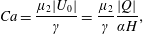 $$\begin{eqnarray}\displaystyle & \displaystyle Ca=\frac{\unicode[STIX]{x1D707}_{2}|U_{0}|}{\unicode[STIX]{x1D6FE}}=\frac{\unicode[STIX]{x1D707}_{2}}{\unicode[STIX]{x1D6FE}}\frac{|Q|}{\unicode[STIX]{x1D6FC}H}, & \displaystyle\end{eqnarray}$$
where
 $U_{0}$
is the velocity at the top (widest) part of the channel, and
 $\text{sgn}(Q)=Q/|Q|$
. In the rest of the paper, the volume flux is taken to be negative (from the wider into the narrower part of the channel), so
 $\text{sgn}(Q)=-1$
.
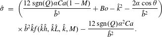
We can now write the dispersion relation, in dimensionless form, as
 $$\begin{eqnarray}\displaystyle \hat{\unicode[STIX]{x1D70E}} & = & \displaystyle \left(\frac{12\,\text{sgn}(Q)\unicode[STIX]{x1D6FC}Ca(1-M)}{\hat{b}^{3}}+Bo-\hat{k}^{2}-\frac{2\unicode[STIX]{x1D6FC}\cos \unicode[STIX]{x1D703}}{\hat{b}^{2}}\right)\nonumber\\ \displaystyle & & \displaystyle \times \,\hat{b}^{2}\hat{k}f(\hat{k}{\hat{h}},\hat{k}\hat{L},\hat{k},M)-\frac{12\,\text{sgn}(Q)\unicode[STIX]{x1D6FC}^{2}Ca}{\hat{b}^{2}}.\end{eqnarray}$$
For convenience, henceforth, we drop the hats from our dimensionless variables: all variables are non-dimensional.
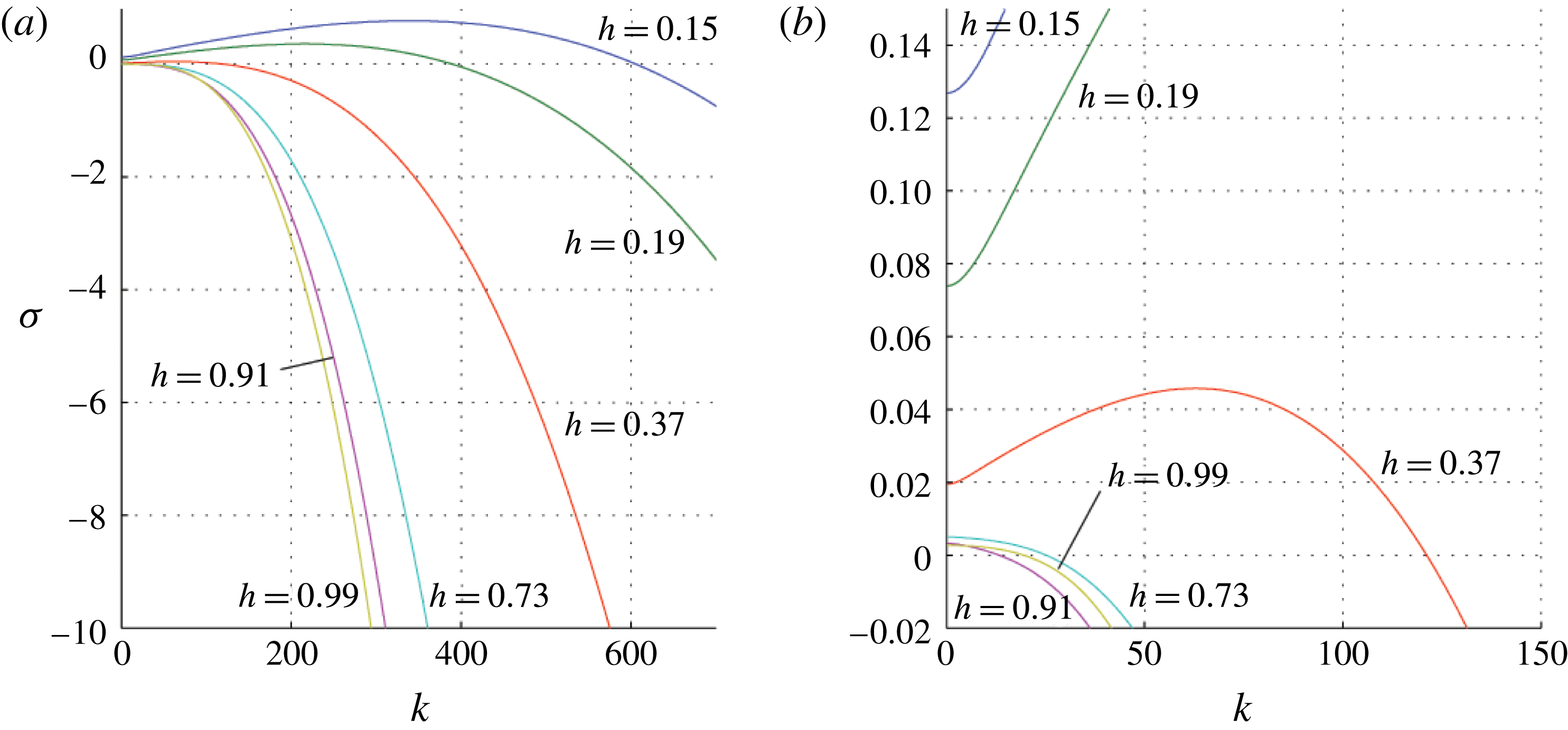
3 Saffman–Taylor instability
Variation of
 $\unicode[STIX]{x1D70E}$
as a function of
 $k$
(2.21) for the case
 $M=1.5$
,
 $Ca=2.2\times 10^{-5}$
,
 $\text{sgn}(Q)=-1$
,
 $Bo=0$
,
 $\unicode[STIX]{x1D6FC}=0.001$
and
 $L=0.1$
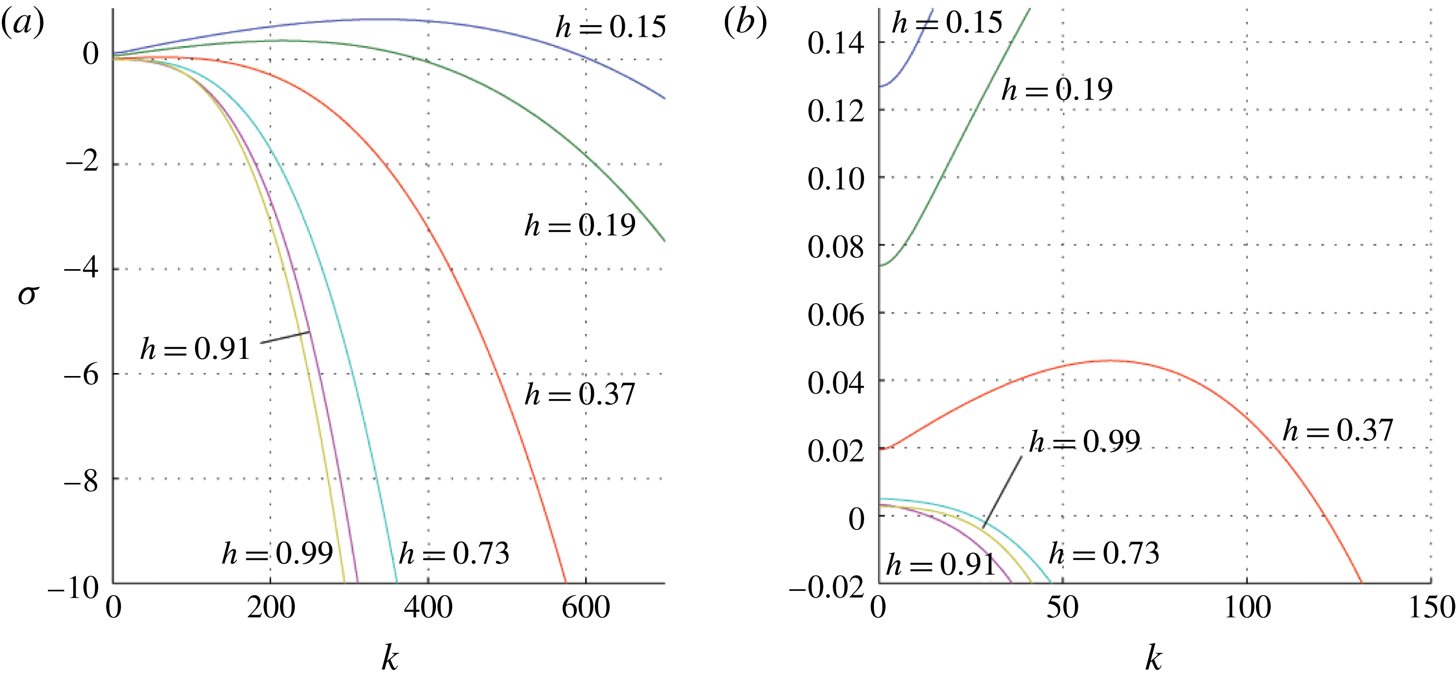
. The blue (
 $h=0.15$
), green (
 $h=0.19$
) and red (
 $h=0.37$
) lines represent small
 $h$
values and show that there is a region of instability; the cyan (
 $h=0.73$
), magenta (
 $h=0.91$
) and yellow (
 $h=0.99$
) lines represent large
 $h$
values for which the flow is stable for all
 $k$
, except for a geometric instability at very long wavelengths. Panel (a) illustrates that for large
 $k$
stability increases with
 $h$
, while panel (b) shows the detail at small
 $k$
and small growth rate
 $\unicode[STIX]{x1D70E}$
. Note that each value of
 $h$
has a particular value of
 $k=k_{c}$
for which
 $\unicode[STIX]{x1D70E}(k_{c})=0$
and such that if
 $k>k_{c}$
all modes are stable.
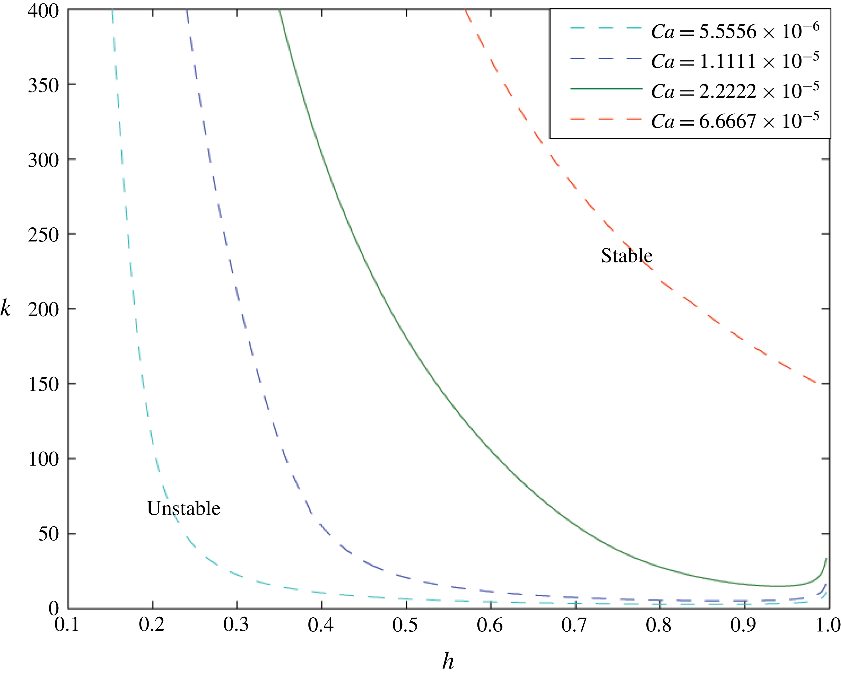
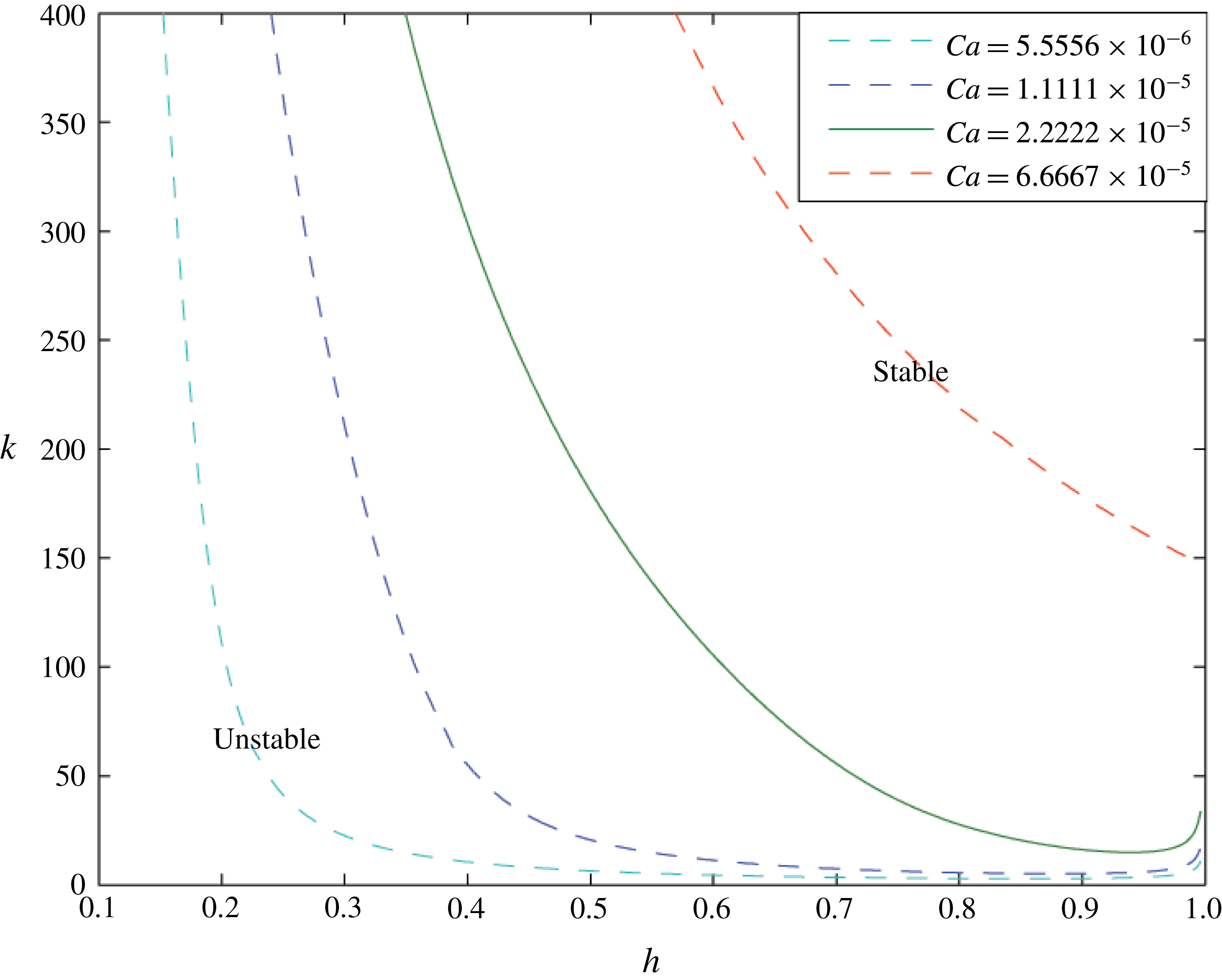
Variation of the critical wavenumber
 $k_{c}$
for neutral stability as a function of
 $h$
for four values of the capillary number
 $Ca$
as indicated in the legend. For
 $k>k_{c}$
the system is stable, whereas for
 $k<k_{c}$
the system is unstable. The solid green line corresponds to
 $Ca=2.2\times 10^{-5}$
. In this figure
 $M=1.5$
and
 $\unicode[STIX]{x1D6FC}=1\times 10^{-4}$
.
In figure 2 we illustrate the dispersion relations for a selection of values of the interface position
 $h$
, for the case
 $M=\unicode[STIX]{x1D707}_{1}/\unicode[STIX]{x1D707}_{2}=1.5$
,
 $\text{sgn}(Q)=-1$
,
 $Bo=0$
and
 $L=0.1$
, so that the less viscous fluid is displacing the more viscous fluid. Figure 2(a) shows the dispersion relation over a wide range of values of
 $\unicode[STIX]{x1D70E}$
and
 $k$
, while figure 2(b) illustrates the detail for small
 $k$
and
 $\unicode[STIX]{x1D70E}$
. The curve
 $h=0.15$
corresponds to the smallest value of
 $h$
shown on the figure and can be seen in blue: there is a range of values of
 $k$
for which
 $\unicode[STIX]{x1D70E}>0$
, illustrating that the interface is unstable for this value of
 $h$
, and for these small values of
 $h$
, the maximum value of
 $\unicode[STIX]{x1D70E}$
occurs when
 $k>0$
. This most unstable mode is associated with the ST instability. As
 $h$
increases, the range of values of
 $k$
for which there is stability increases, and eventually only the longest-wavelength modes remain unstable. The maximum value of
 $\unicode[STIX]{x1D70E}$
now occurs when
 $k=0$
, and this is the instability associated with the convergence of the flow in the channel.
In the narrower parts of the cell, which correspond to the smaller values of
 $h$
, the flow speed is larger and this enhances the viscous destabilisation of the interface: decreasing
 $h$
and hence the channel width increases the range of
 $k$
for which the growth rate
 $\unicode[STIX]{x1D70E}$
is positive.
There is a critical wavenumber
 $k_{c}$
such that for
 $k>k_{c}$
the system is stabilised by perturbation surface tension: this wavenumber
 $k_{c}$
is dependent on
 $h$
and can be seen in figure 2 by the point at which each curve intersects the
 $\unicode[STIX]{x1D70E}=0$
line. For example, for
 $h=0.15$
this critical wavenumber is approximately 600. In figure 3 the green line illustrates the variation of this critical wavenumber with
 $h$
for
 $Ca=2.2\times 10^{-5}$
. For a given
 $h$
, the interface is stable for
 $k>k_{c}(h)$
, and unstable for
 $k<k_{c}(h)$
. For a given value of
 $h$
, this critical wavenumber
 $k_{c}$
also varies with capillary number. In figure 3 the dashed cyan line corresponds to
 $Ca=5.6\times 10^{-6}$
, the dashed blue line to
 $Ca=1.1\times 10^{-5}$
and the red line to
 $Ca=6.7\times 10^{-5}$
. The higher the capillary number, the greater the region of instability both in wavenumber
 $k$
and in regions of the channel
 $h$
. However, the flow is never absolutely stable, since, as for very small wavelengths, the dominant effect is the destabilising geometric instability due to the flow accelerating quasi-statically as it moves into the narrower part of the channel. For modes of higher wavenumber we expect that the interface in a flow migrating towards the wider part of the channel may transition from instability to stability, whereas a flow which migrates to the narrow part of the channel may transition from stability to instability.
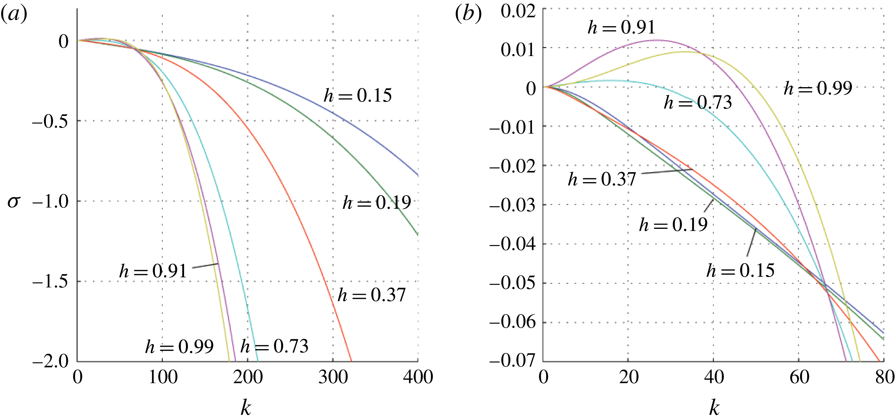
4 Rayleigh–Taylor instability
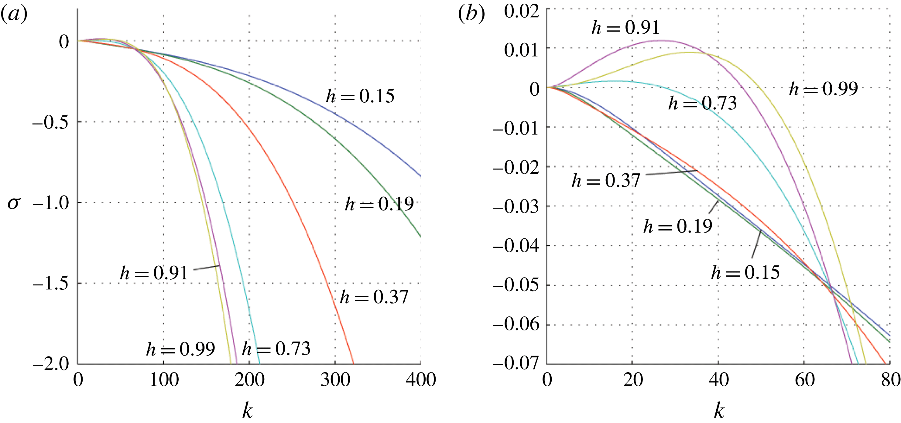
Variation of
 $\unicode[STIX]{x1D70E}$
as a function of
 $k$
(2.21) for the case
 $M=1.5$
,
 $Bo=4500$
,
 $\unicode[STIX]{x1D6FC}=0.001$
and
 $Ca=0$
. The blue (
 $h=0.15$
), green (
 $h=0.19$
) and red (
 $h=0.37$
) lines represent small values of
 $h$
for which the flow is stable. The cyan (
 $h=0.73$
), magenta (
 $h=0.91$
) and yellow (
 $h=0.99$
) lines represent larger values of
 $h$
. For each of these cases, there is a range of values of
 $k$
for which
 $\unicode[STIX]{x1D70E}>0$
and the flow is unstable. Again, panel (b) shows that for large
 $k$
the flow becomes progressively more stable as
 $h$
increases, while panel (a) shows the behaviour near the origin.
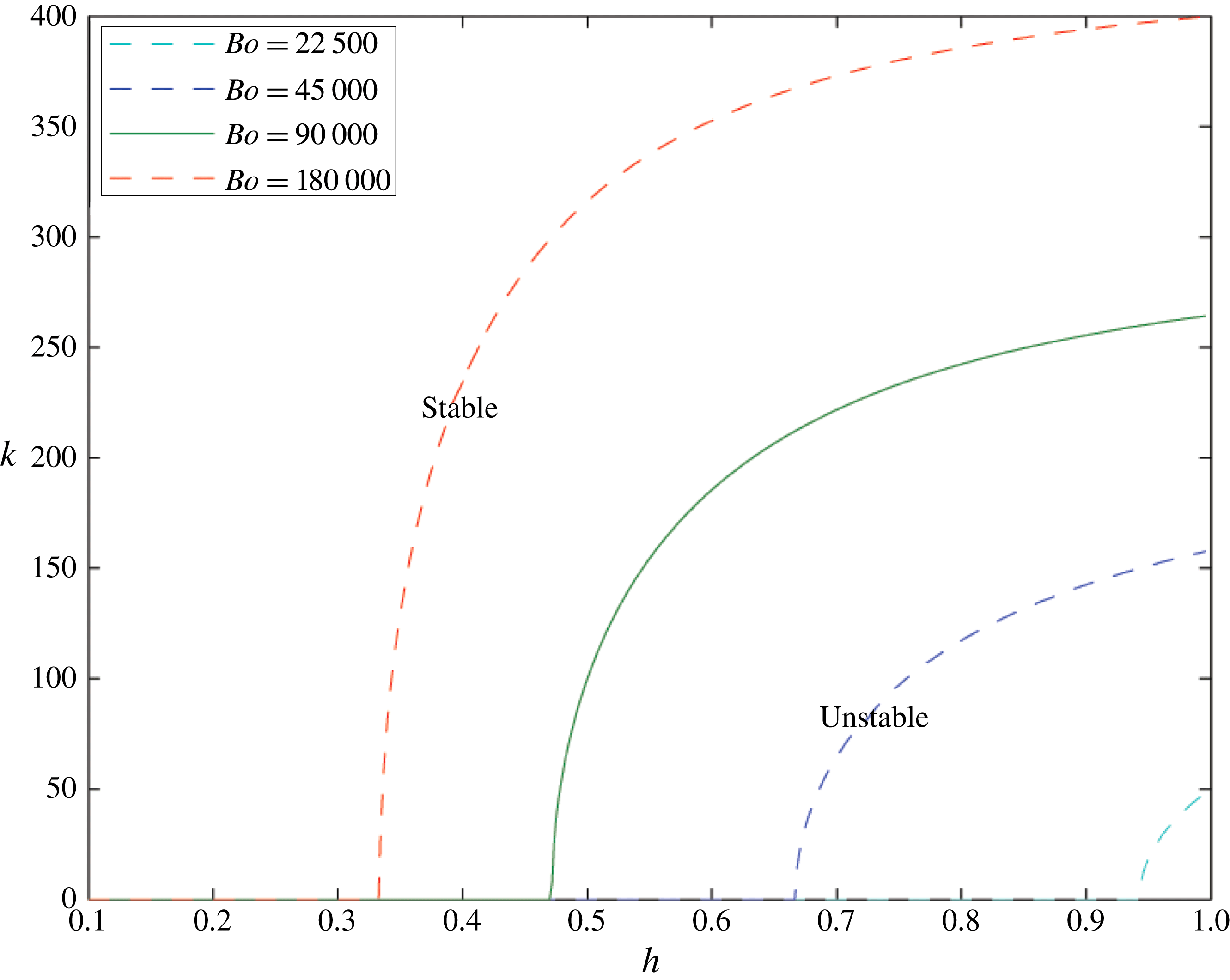
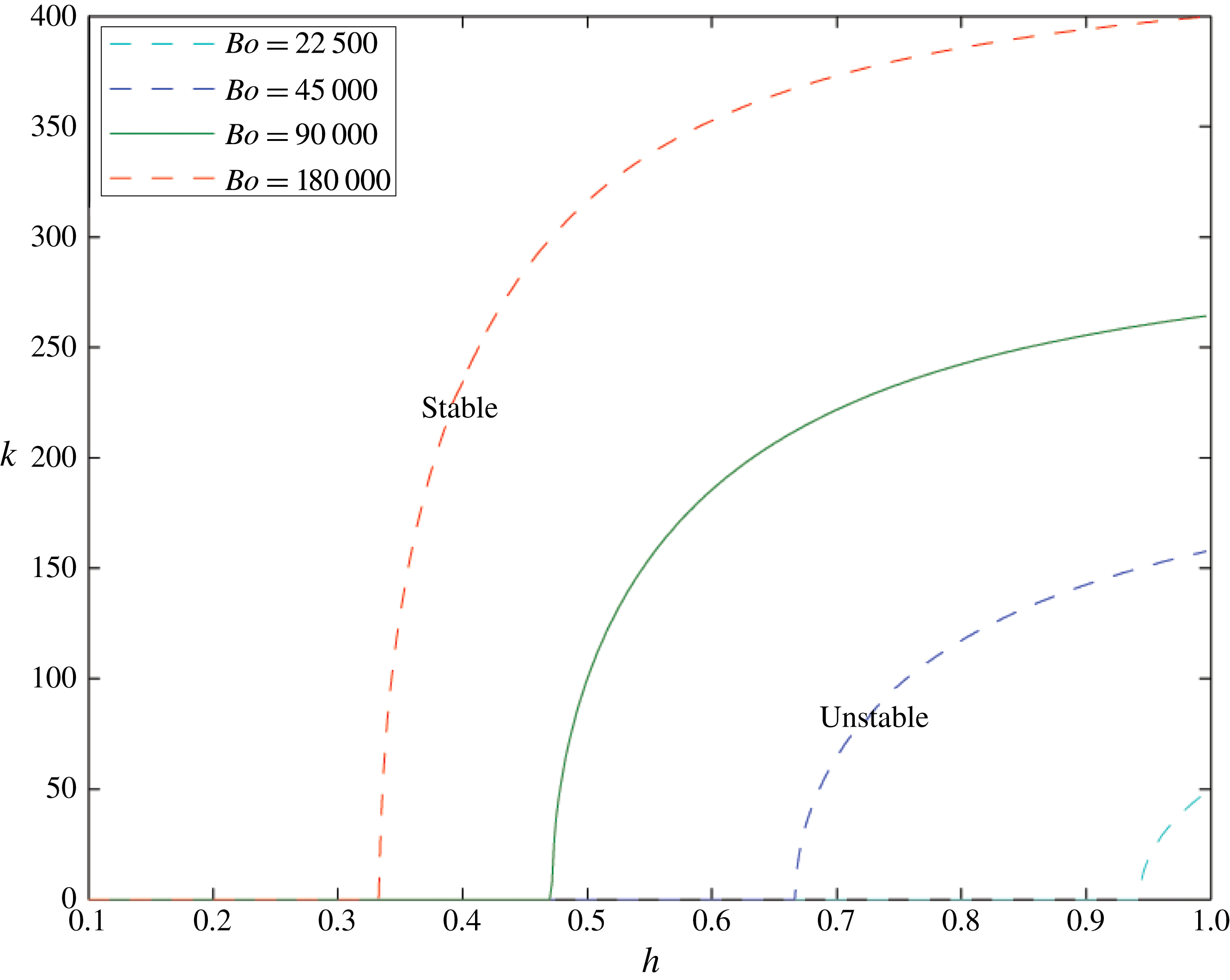
For a specific Bond number and given interface height
 $h$
there is a critical wavenumber above which the perturbation surface tension stabilises all modes. This wavenumber for
 $Bo=9\times 10^{4}$
is shown in green; if surface tension stabilises all modes with a wavenumber greater than 0, then the interface is absolutely stable, which we can see for
 $0.1<h<0.47$
. For smaller wavenumbers or greater interface heights than the critical value, the interface is unstable to a RT instability. Equivalent curves for different Bond numbers are also shown in cyan, blue and red. The smaller the Bond number, the smaller is the unstable region, and the higher the interface needs to be for the instability to manifest. Here
 $M=1.5$
and
 $\unicode[STIX]{x1D6FC}=1\times 10^{-4}$
.
We now consider a cell with zero capillary number (
 $Q=0$
), but with
 $Bo=4.5\times 10^{4}$
and
 $L=0.1$
. Figure 4 shows the dispersion relation for a series of values of
 $h$
. Figure 4(b) shows the same results as figure 4(a) but zoomed in on the detail at small
 $\unicode[STIX]{x1D70E}$
. The cases
 $h=0.99$
,
 $0.91$
and
 $0.73$
all include a range of values of
 $k$
for which
 $\unicode[STIX]{x1D70E}>0$
and the interface is unstable. In contrast, for smaller values of
 $h=0.15$
,
 $0.19$
and
 $0.37$
(hence narrower channel width), figure 4 illustrates that
 $\unicode[STIX]{x1D70E}<0$
for all
 $k$
and the system is absolutely stable. The in-channel surface tension stabilises the system when the channel thickness is small. We see that as
 $h\rightarrow 1$
the growth rate
 $\unicode[STIX]{x1D70E}$
becomes progressively more negative. The growth rate is zero when
 $k=0$
since with no flow (
 $Q=0$
) there is no geometric instability.
The solid green line in figure 5 again shows the critical wavenumber above which all modes are stable. The absence of the geometric instability leads to a range of
 $h$
for which the flow is absolutely stable (where the green line meets the
 $x$
axis). Equivalent results are shown for
 $Bo=2.25\times 10^{4}$
(cyan),
 $Bo=9\times 10^{4}$
(blue) and
 $Bo=1.8\times 10^{5}$
(red). We see that increasing
 $Bo$
reduces the range of interface heights which are absolutely stable as a result of the in-channel surface tension. For large
 $h$
, increasing
 $Bo$
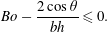
also reduces the number of stable modes: only very short-wavelength disturbances are stabilised by surface tension. With no flow, (2.21) shows that we have absolute stability when
 $$\begin{eqnarray}Bo-\frac{2\cos \unicode[STIX]{x1D703}}{bh}\leqslant 0.\end{eqnarray}$$
5 Combined problem
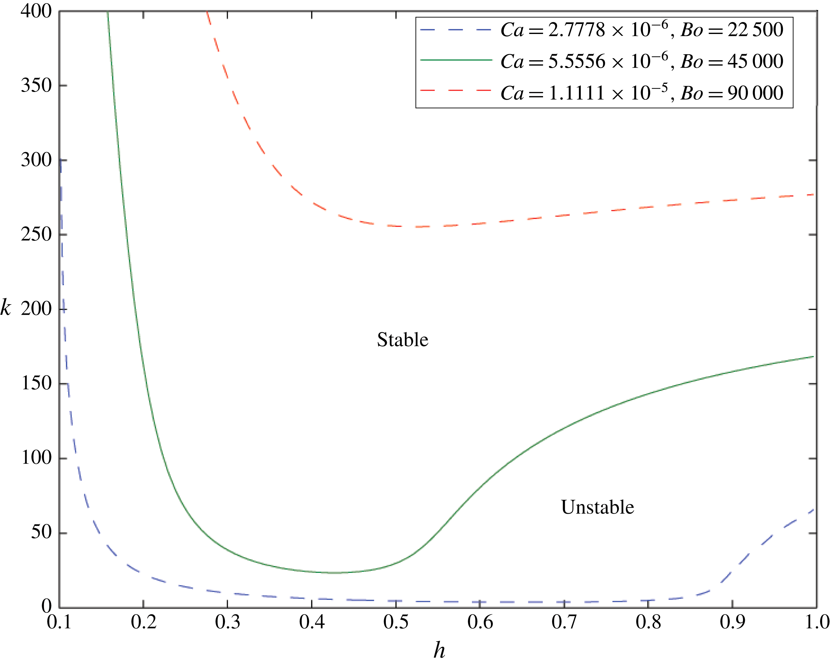
Similarly to figures 3 and 5 the green line shows the critical
 $k=k_{c}$
such that for
 $k>k_{c}$
all modes are stabilised by surface tension, in the case that
 $Ca=5.6\times 10^{-6}$
and
 $Bo=4.5\times 10^{4}$
, and
 $\text{sgn}(Q)=-1$
. The interface is unstable to a variety of modes for both large
 $h>0.55$
and small
 $h<0.25$
. These are connected by a predominantly stable region. In the small
 $h$
domain the system is unstable to ST fingering. In the large
 $h$
domain the flow is unstable to a RT-type instability. In the central region the in-channel surface tension stabilises both the ST and RT modes, but the geometric instability still dominates for small
 $k$
. A similar picture arises for other values of capillary/Bond number pairs: they vary at the same rate representing a change in the strength of surface tension. Here
 $M=1.5$
and
 $\unicode[STIX]{x1D6FC}=1\times 10^{-4}$
.
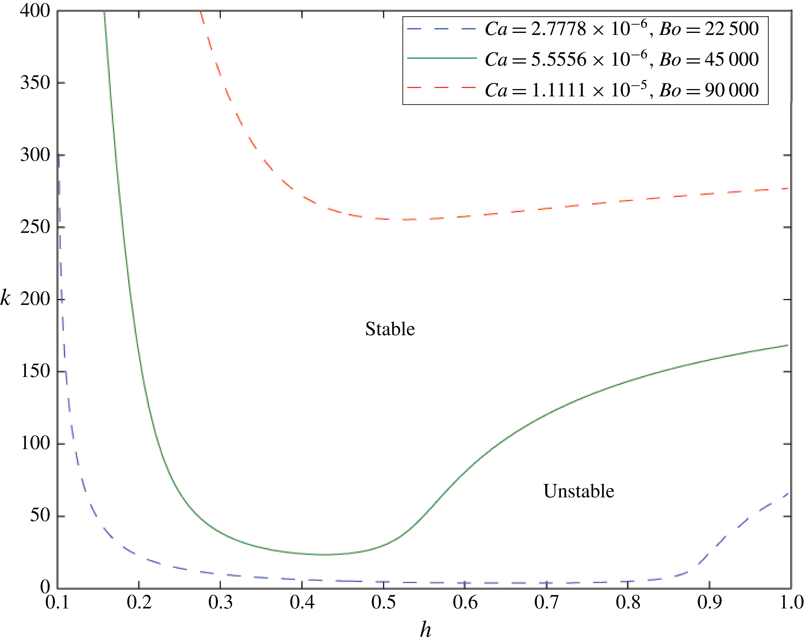
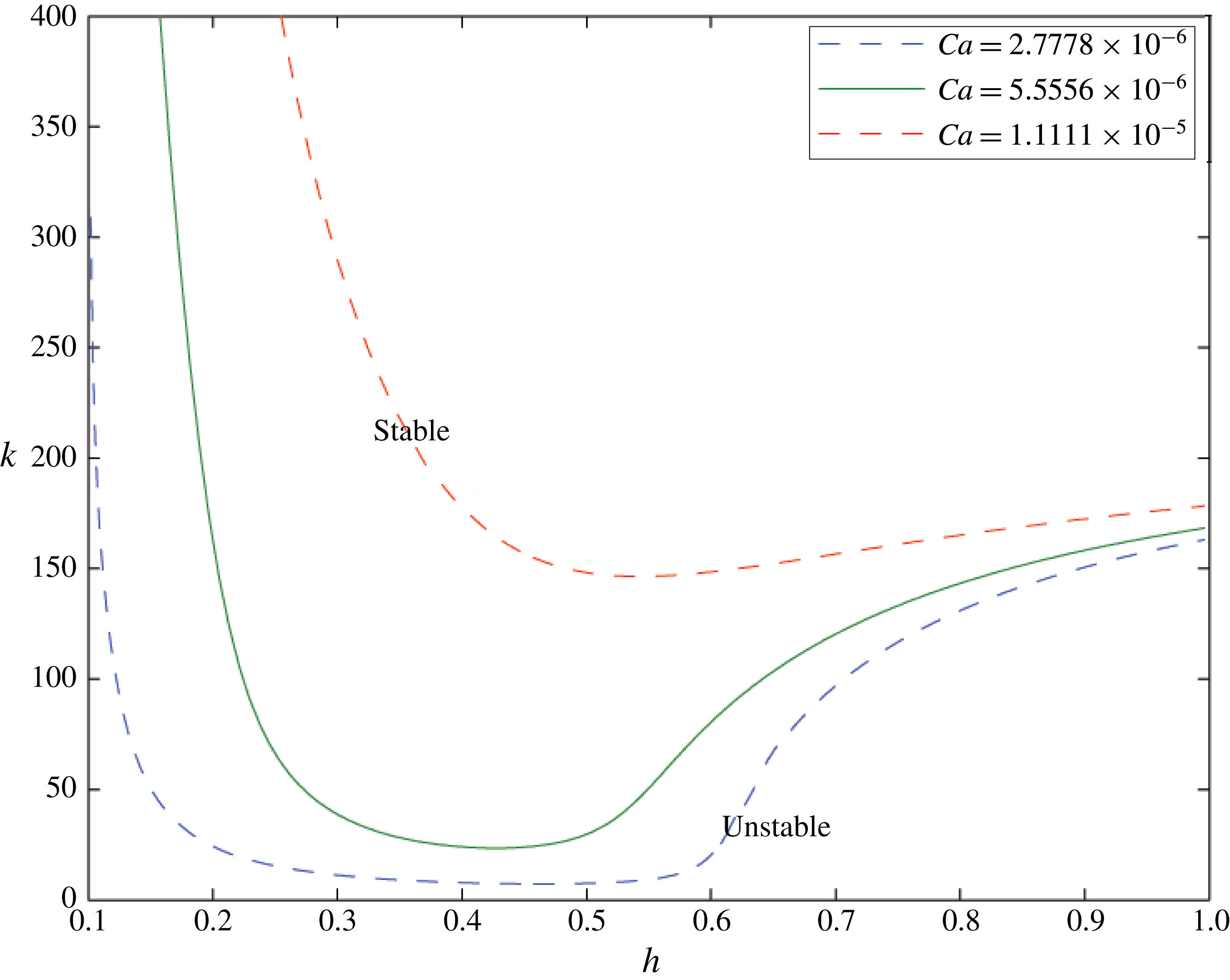
As in figure 6 the green line shows the critical wavenumber above which the interface is stable for
 $Ca=5.6\times 10^{-6}$
and
 $\text{sgn}(Q)=-1$
. In this figure the other lines show the equivalent results when the Bond number is held constant at
 $Bo=4.5\times 10^{4}$
and the capillary number is varied. We see that the behaviour near the wider part of the channel (large
 $h$
) is broadly similar while there are big differences in stability for small
 $h$
: this is where the ST instability is expected to develop. Here
 $M=1.5$
and
 $\unicode[STIX]{x1D6FC}=1\times 10^{-4}$
.
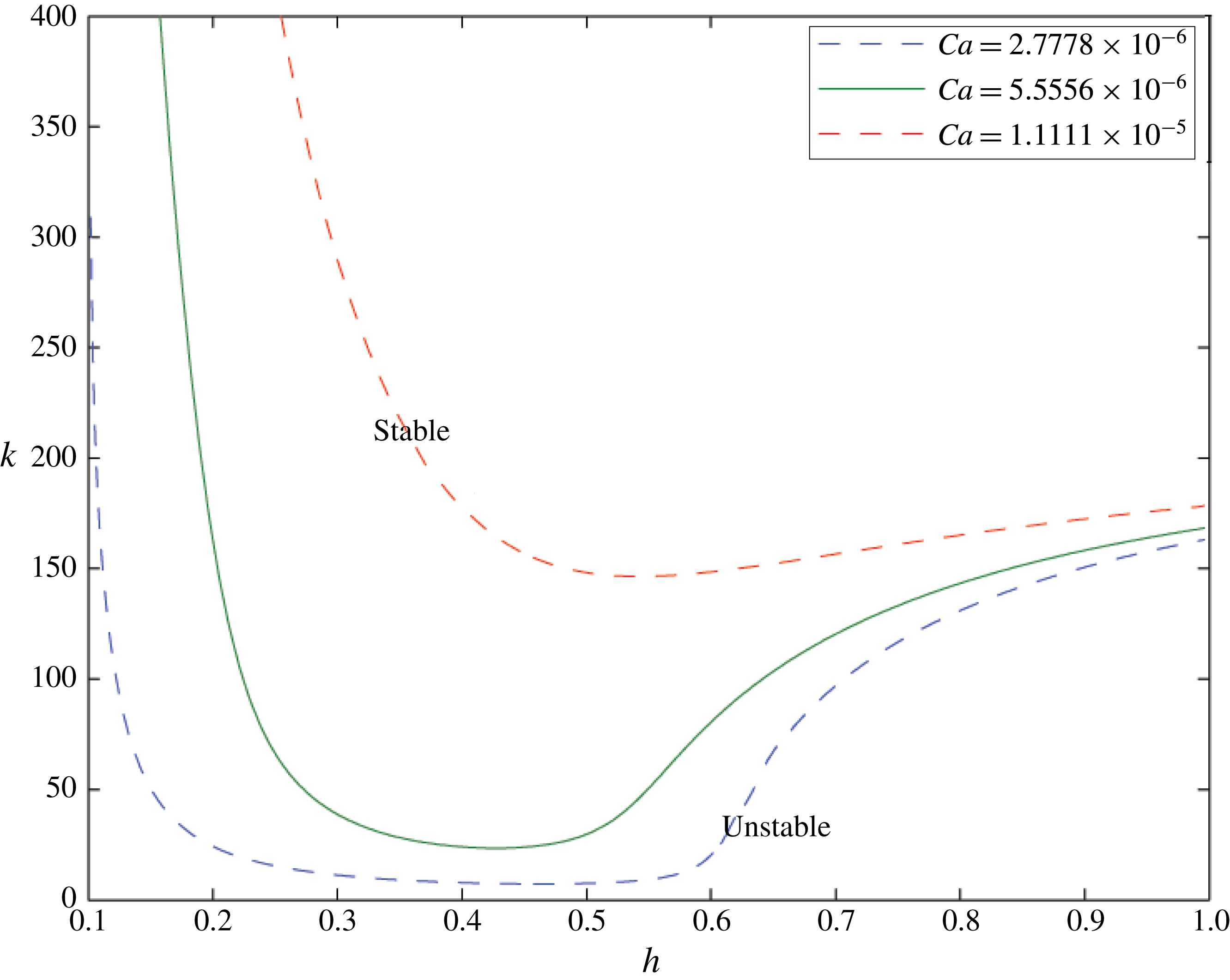
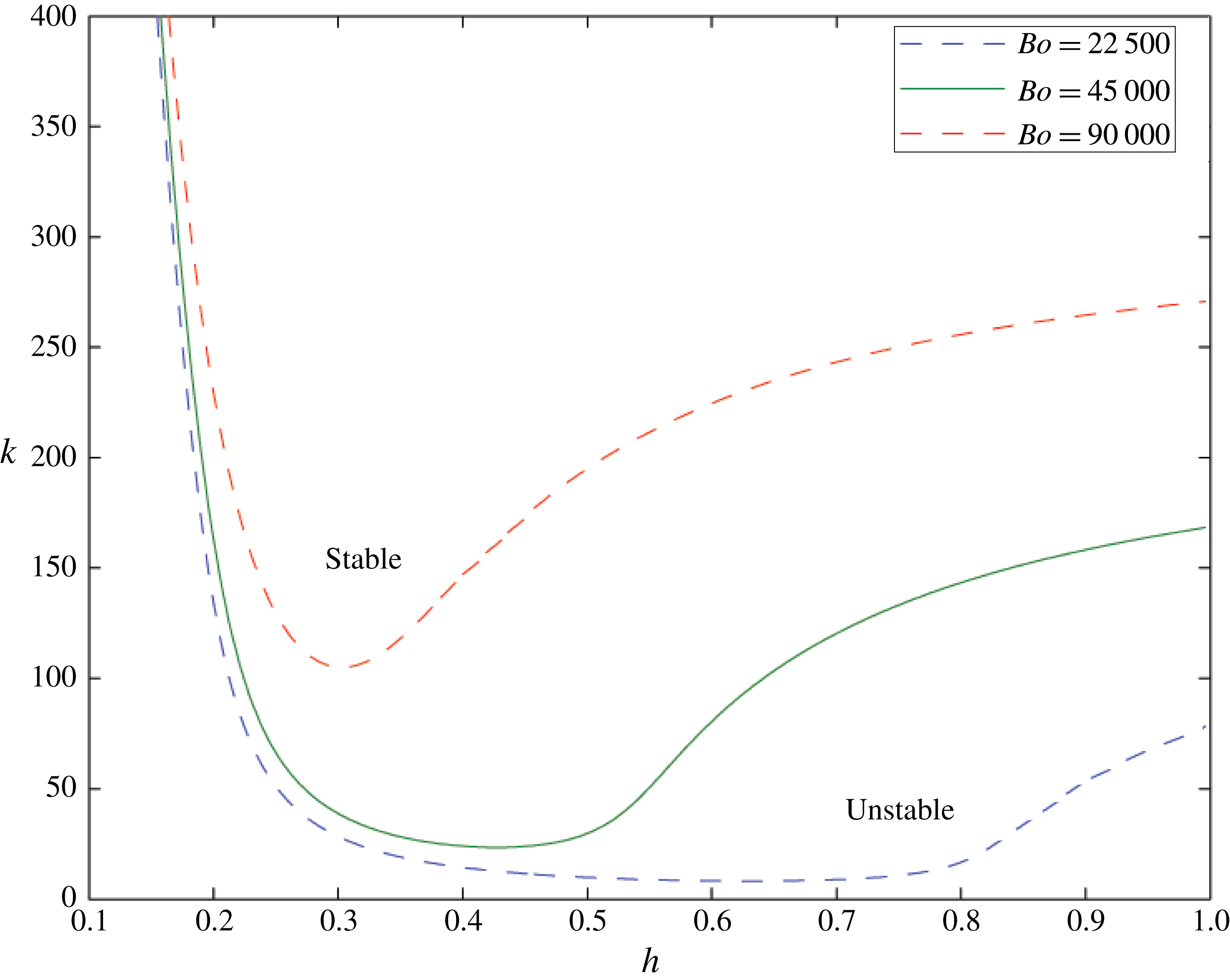
The equivalent to figure 7: the green line again shows the critical wavenumber above which the interface is stable for
 $Bo=45\,000$
,
 $Ca=5.6\times 10^{-6}$
and
 $\text{sgn}(Q)=-1$
. Here the other lines show the equivalent results when the capillary number is held constant and the Bond number is varied. This time the behaviour of the different lines differs for large
 $h$
as the density difference is more important in the wider section of the channel, while the stability behaviour is similar for small
 $h$
. Here
 $M=1.5$
and
 $\unicode[STIX]{x1D6FC}=1\times 10^{-4}$
.
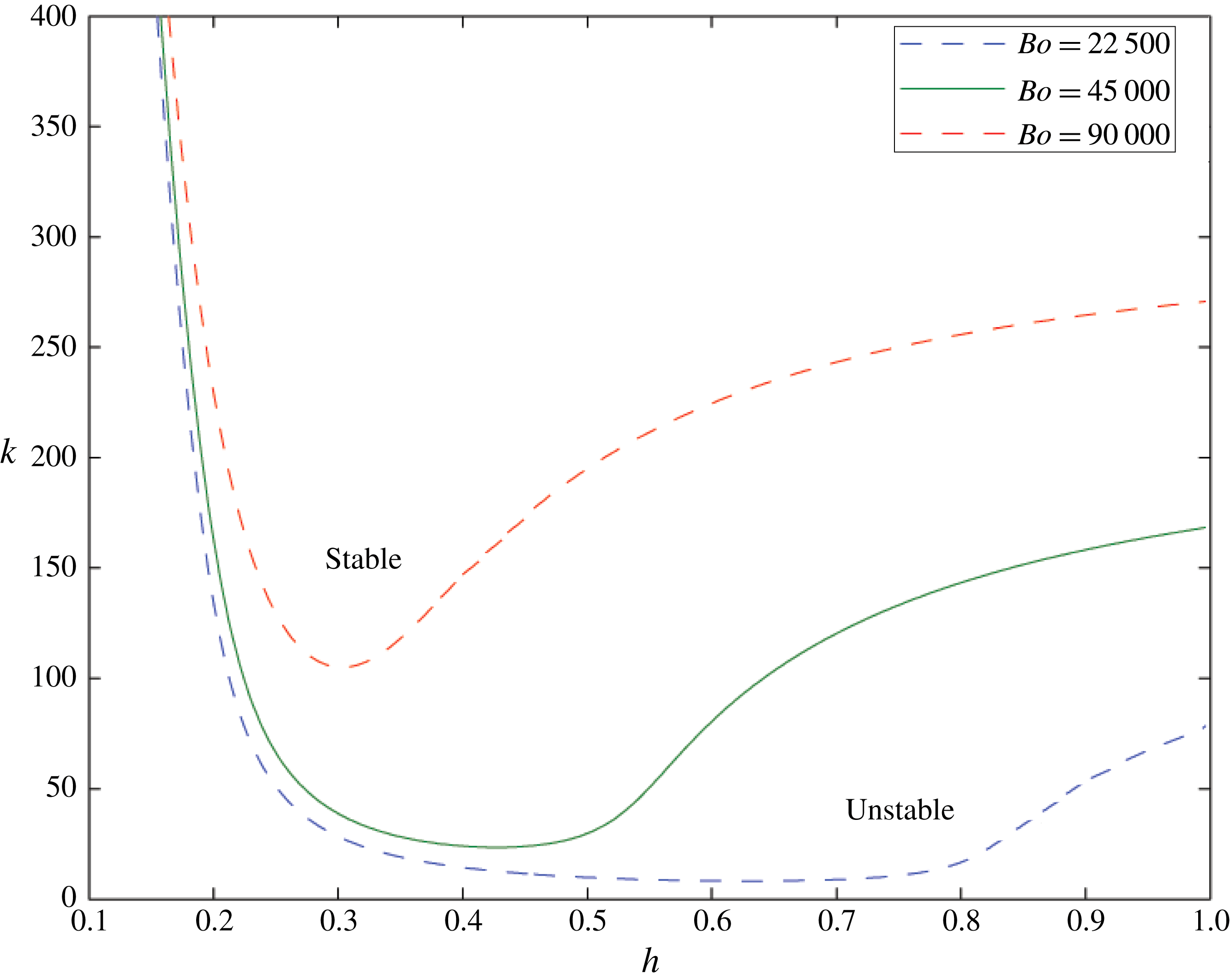
Figures 2 and 4 show that the two different instabilities are quite distinct, and when they are combined we anticipate that, if an interface migrates through a converging channel, the flow may initially be unstable to RT instability, but then may become stabilised by the effect of in-channel surface tension (except for the very long-wavelength modes which continue to be destabilised by the converging walls of the channel), while finally the interface becomes unstable to ST instability in the narrowest part of the cell where the flow speed is highest.
To illustrate this change in the stability of the system, figures 6–8 show the stable and unstable wavenumbers at different interface heights within the channel for a selection of capillary and Bond numbers. The solid green line in each figure uses the same capillary and Bond numbers. Modes with wavenumber greater than the wavenumber on the green line are stabilised while those with smaller wavenumber are destabilised. Figure 6 shows equivalent lines in which both the capillary and Bond numbers are varied, as a result of changing surface tension alone. We can see that the stronger the surface tension, the smaller are the regions that are unstable to RT (large
 $h$
) and ST (small
 $h$
) instability.
In figure 7 we keep the Bond number the same. The wide channel behaviour is very similar for all capillary numbers: the effect of changing the flow speed has only a small impact here. However, in the narrower part of the channel, the region of ST instability becomes markedly bigger as the capillary number is increased.
Conversely figure 8 illustrates that when we change the Bond number but keep the capillary number constant, and thereby change the strength of the RT instability, the stability regime diagram remains similar in the narrow part of the channel, but changes in the wider part of the channel, where the effect of the RT instability is dominant.
As mentioned in § 3, in all cases, a region of instability persists for very small
 $k$
owing to the growth of modes associated with the convergence of the channel. In a cell of sufficiently small finite cross-flow size, this effect will not be seen, but we include it in the analysis and results for completeness.
6 Constant pressure drop
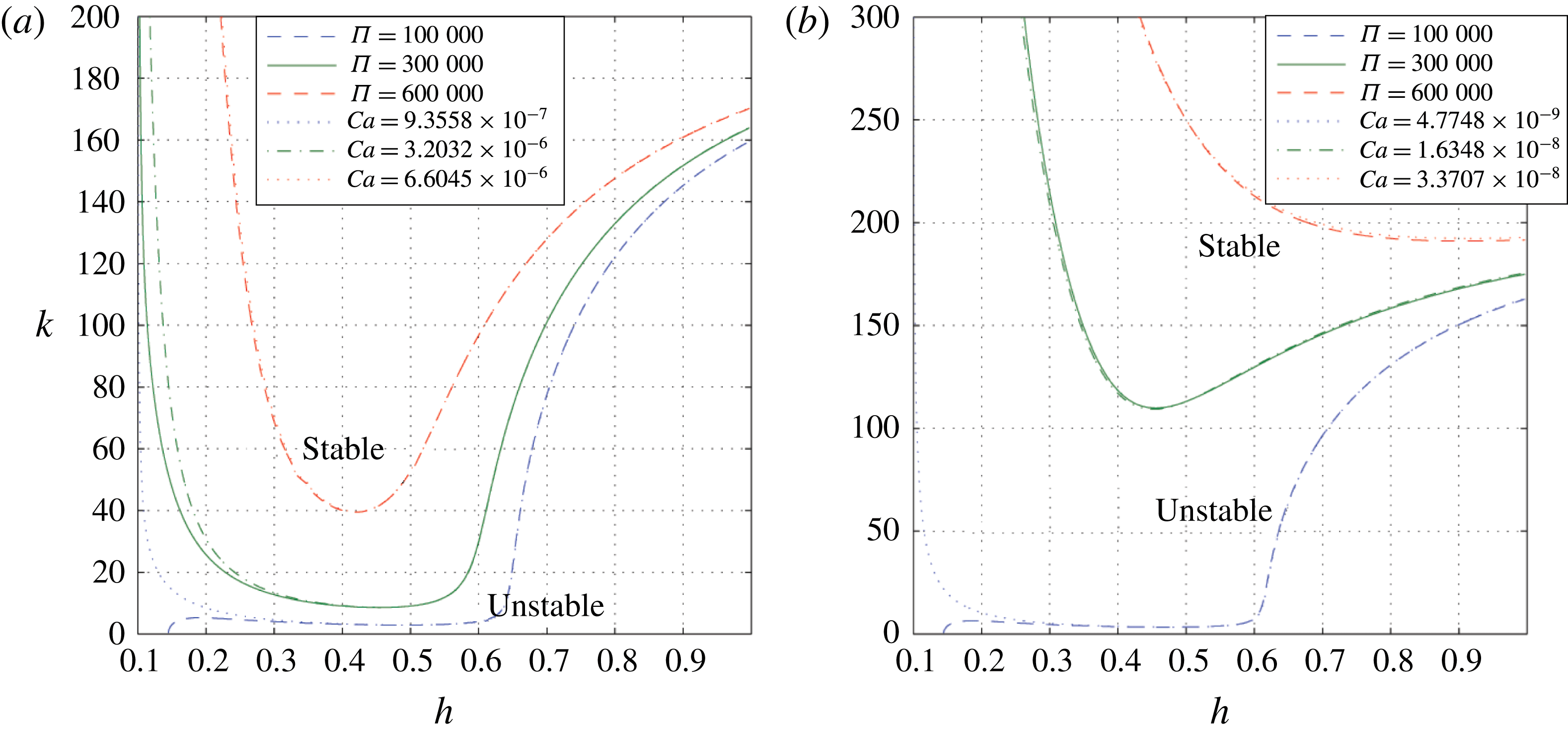
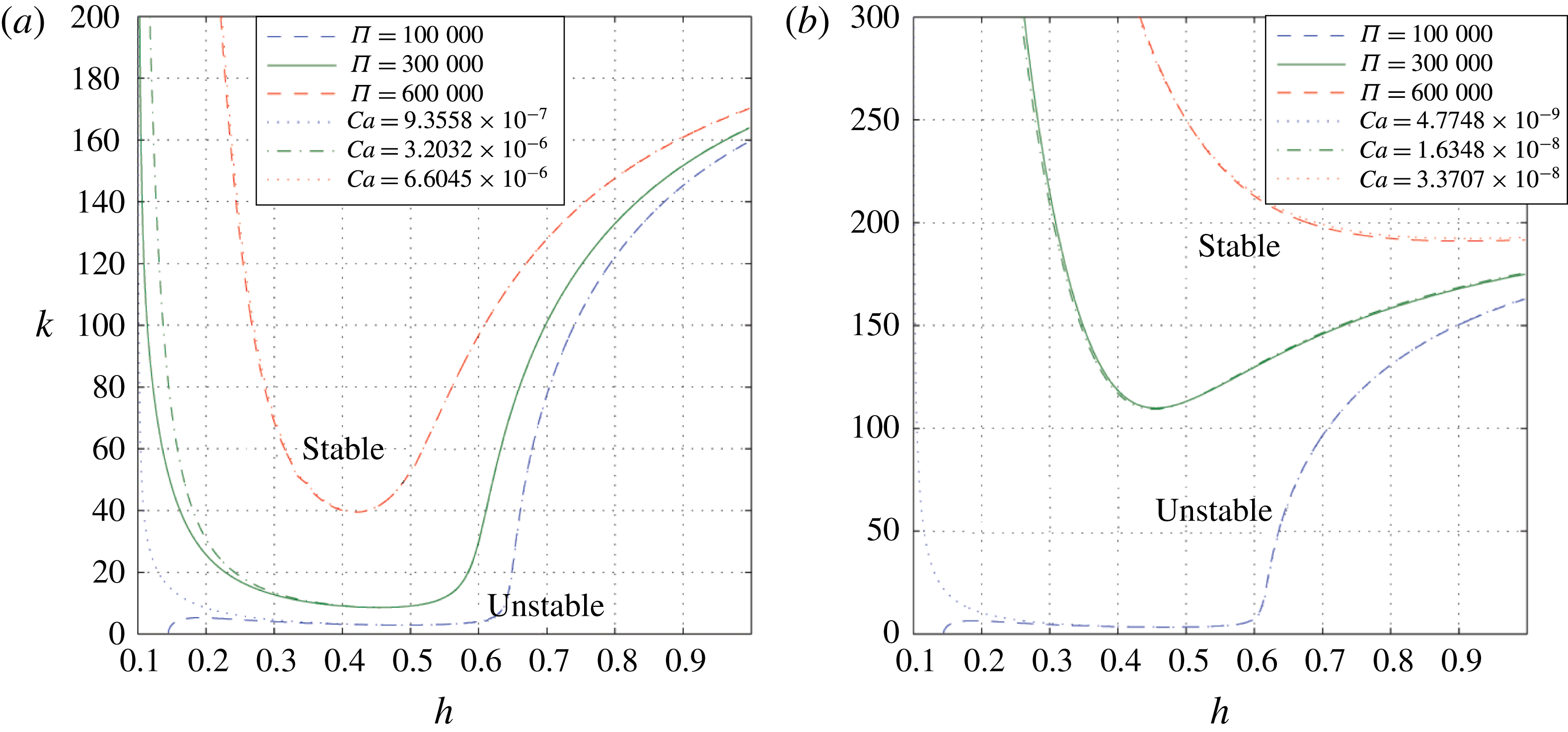
An equivalent plot to figure 6, showing in solid green the critical wavenumber above which the interface is stable for the case that the pressure drop is held constant over the cell (
 $\unicode[STIX]{x1D6F1}=3\times 10^{5}$
). Modes above this line are stable; those below are unstable. For comparison, the equivalent constant volume flux result (
 $Ca=3.2\times 10^{-6}$
) is shown in dash-dotted green, chosen so that the flow speeds in both cases are equal at
 $h=0.5$
. Critical wavenumber lines for different values of
 $\unicode[STIX]{x1D6F1}$
are shown in dashed blue and red, as well as their equivalent capillary number cases in dotted blue and red. Panel (a) shows the results for
 $M=1.5$
while panel (b) shows the results for
 $M=300$
. Here
 $\unicode[STIX]{x1D6EC}=20$
,
 $Bo=4.5\times 10^{4}$
and
 $\unicode[STIX]{x1D6FC}=1\times 10^{-4}$
.
In this paper, we have assumed a constant volume flux through the channel. An alternative approach could be to hold the pressure drop across the channel constant. Then we expect the volume flux to change as the ratio of more viscous to less viscous fluid in the cell changes. We introduce two new dimensionless numbers corresponding to the Bond and capillary numbers, respectively:
 $$\begin{eqnarray}\displaystyle & \displaystyle \unicode[STIX]{x1D6EC}=\frac{gH^{2}\unicode[STIX]{x1D70C}_{1}}{\unicode[STIX]{x1D6FE}}, & \displaystyle\end{eqnarray}$$
 $$\begin{eqnarray}\displaystyle & \displaystyle \unicode[STIX]{x1D6F1}=\frac{\unicode[STIX]{x0394}pH}{\unicode[STIX]{x1D6FE}}, & \displaystyle\end{eqnarray}$$
where
 $\unicode[STIX]{x0394}p$
is the difference in pressure between the top and the bottom of the cell. If we solve for the flow with the constant pressure boundary conditions, we find an expression for an equivalent capillary number based on
 $\unicode[STIX]{x1D6EC}$
,
 $\unicode[STIX]{x1D6F1}$
and
 $h$
:
 $$\begin{eqnarray}Ca=\left|\frac{b^{2}L^{2}(\unicode[STIX]{x1D6F1}+Bo(1-h)+\unicode[STIX]{x1D6EC}(1-L)-2\cos \unicode[STIX]{x1D703}/b)}{6(h^{2}L^{2}-(1-M)L^{2}-h^{2}M)}\right|.\end{eqnarray}$$
Figure 9 shows two comparison plots of the critical wavenumber
 $k$
corresponding to the case of neutral stability as a function of
 $h$
, for
 $M=1.5$
in figure 9(a) and for
 $M=300$
in figure 9(b). The solid green line shows the case in which
 $\unicode[STIX]{x1D6F1}=3\times 10^{5}$
corresponding to a constant pressure drop across the channel. For a given interface height, the flow is unstable if
 $k<k_{c}$
, where neutrally stable
 $k_{c}$
is shown as the green line, and the system is unstable if
 $k>k_{c}$
. The dashed blue and red lines represent the corresponding neutral stability curve for these alternative values of
 $\unicode[STIX]{x1D6F1}$
. The dash-dotted green line and dotted blue and red lines show the corresponding calculations for constant
 $Ca$
in which the volume flux through the channel is kept constant, as we have assumed elsewhere in the paper. The values of
 $Ca$
are chosen so that the lines intersect at
 $h=0.5$
: this corresponds to the interface speeds being the same at
 $h=0.5$
.
We see that, except for small
 $h$
, the lines are very similar – for the stability analysis it matters little whether the problem is one of constant volume flux or constant pressure drop, unless the transition between stability and instability is in the narrow part of the channel. One key difference between the cases is that, for a given small pressure change across the cell,
 $\unicode[STIX]{x1D6F1}$
, the flow becomes stable to all wavenumbers for small values of
 $h$
. In the region of the channel narrower than this transition value, the effect of surface tension becomes stronger than the imposed pressure gradient, and so the flow changes direction. In the upward direction the flow is stable both to ST instability and to the geometric instability, leading to this small region of absolute stability.
7 Growth as the interface migrates through the channel
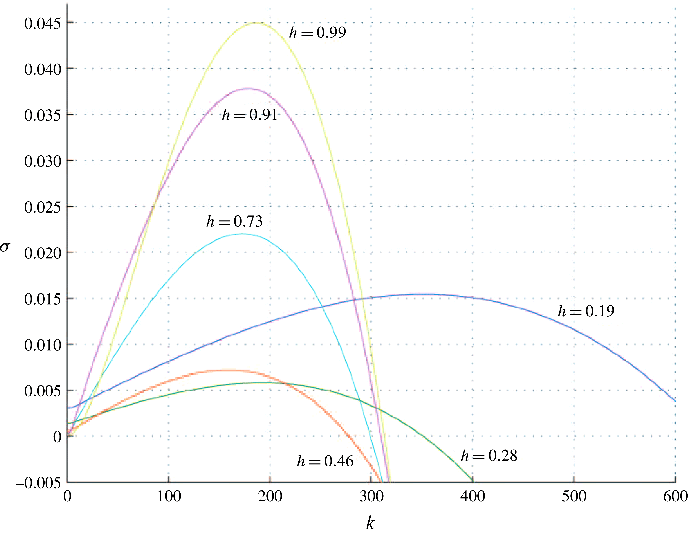
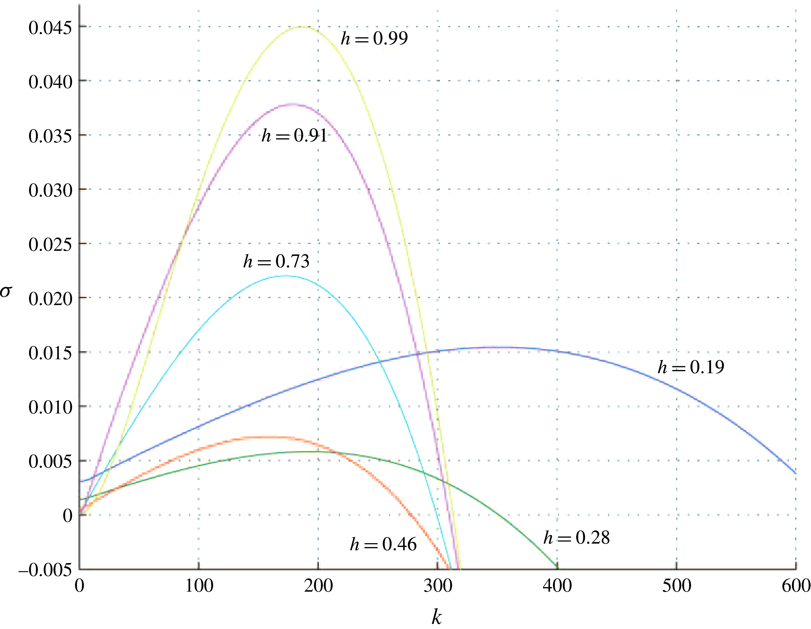
Variation of
 $\unicode[STIX]{x1D70E}$
as a function of
 $k$
(2.21) for the case
 $M=1.5$
,
 $Ca=-9.3\times 10^{-6}$
,
 $\text{sgn}(Q)=-1$
,
 $Bo=1.1\times 10^{5}$
,
 $\unicode[STIX]{x1D6FC}=1\times 10^{-4}$
and
 $L=0.1$
. The blue (
 $h=0.19$
) and green (
 $h=0.28$
) lines represent small
 $h$
values. In these regions the interface is unstable to a ST instability; the range of unstable wavenumbers increases closer to the end of the channel (where the flow is faster). The intermediate
 $h$
values in red (
 $h=0.46$
) and cyan (
 $h=0.73$
) show lower growth rates as both the RT and ST effects are smaller compared to the effect of the in-channel surface tension. Finally, the magenta (
 $h=0.91$
) and yellow (
 $h=0.99$
) lines for large
 $h$
values show an increase in growth rate as well as another increase in the most unstable wavenumber, as both in-channel and perturbation surface tension become weaker compared to the RT instability.
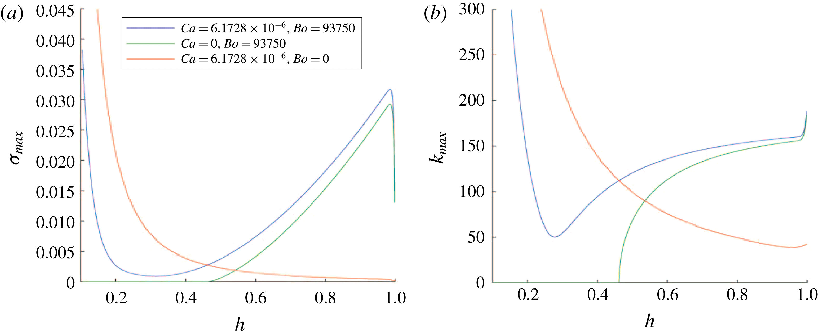
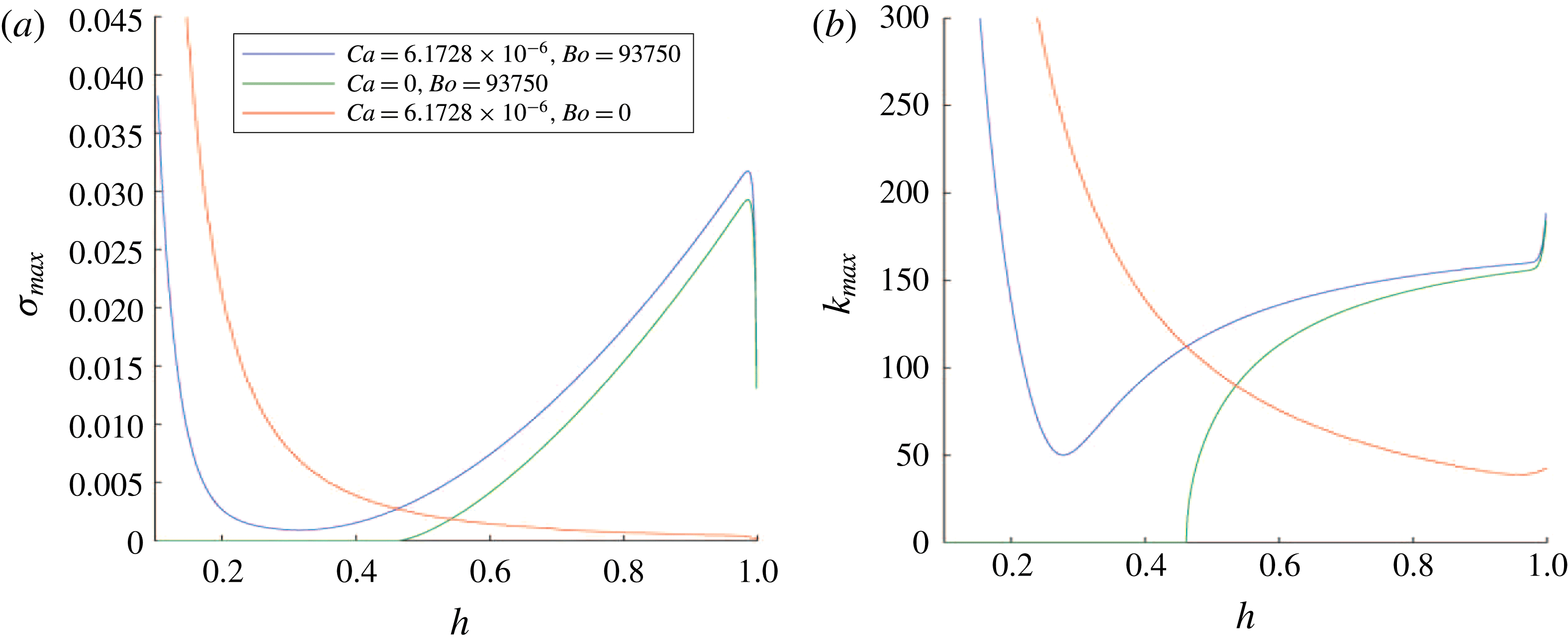
(a) The maximum value over all wavenumbers
 $k$
of the growth rate as a function of
 $h$
. This is displayed for three sets of parameter values. When
 $Ca=0$
(green) there is no ST instability in the narrow part of the channel. When
 $Bo=0$
(red) there is no RT instability in the wide part of the channel. When they are both non-zero (blue) there is a surface tension-induced minimum growth rate in an intermediate section of the channel where ST and RT effects are relatively weak. (b) The wavenumber corresponding to the mode of the maximum growth rate. This wavenumber is 0 when surface tension suppresses the RT instability (shown in green for
 $h<0.46$
) and is close to 0 when surface tension suppresses the ST instability but not the geometric instability (red line). The blue line shows how the surface tension causes the maximal wavenumber to decrease in the centre of the channel, but, as the strength of the ST or RT instability increases at the narrow or wide end of the channel, so does the most unstable wavenumber.
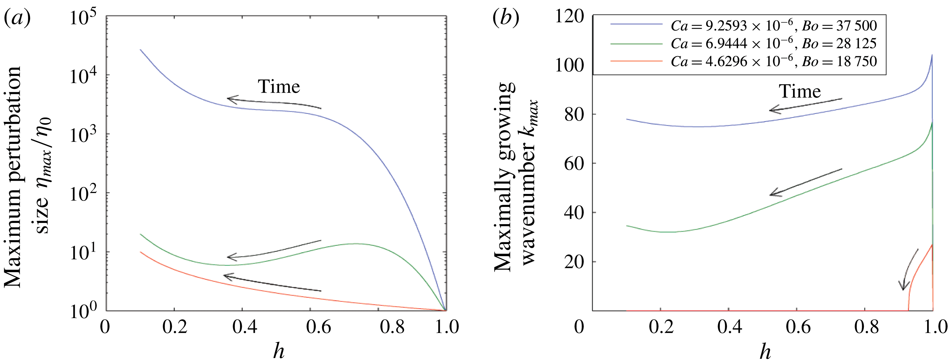
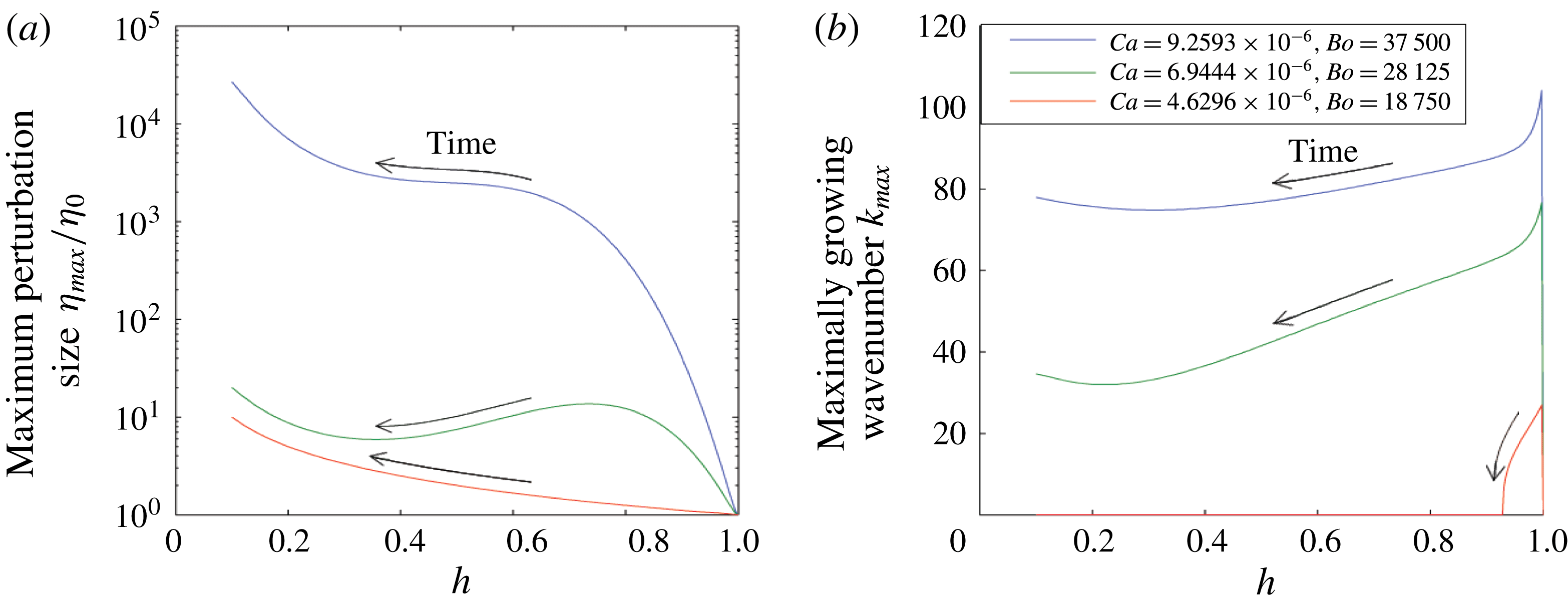
(a) Variation of the magnitude of the mode with the largest amplitude as a function of the height of the interface in the cell
 $h(t)$
for three different sets of capillary and Bond numbers. The arrows indicate the evolution along these curves as a function of time. (b) Variation of the wavenumber of the mode with the largest amplitude as a function of
 $h(t)$
, for the same parameters as in panel (a). The arrows again show the direction of time. While for larger instabilities the most unstable wavenumber changes slowly in time, for
 $Ca=4.6\times 10^{-6}$
and
 $Bo=1.9\times 10^{4}$
the most unstable wavenumber is non-zero only for
 $h>0.92$
. Below this point the in-channel surface tension stabilises the ST and RT modes and the only instability is geometric.
In figure 10 we illustrate how the growth rate as a function of wavenumber can change depending on the position of the interface within the channel. In the wide part of the channel (
 $h=0.99$
,
 $h=0.91$
) the flow is unstable to the RT instability. For intermediate channel widths (
 $h=0.73$
,
 $h=0.46$
) the in-channel surface tension significantly reduces the magnitude of the mode with maximum growth rate. Finally, the interface becomes more unstable again in the narrow part of the channel (
 $h=0.28$
,
 $h=0.19$
) when the ST instability becomes more pronounced owing to the increase in flow speed. The most unstable wavenumber also increases in this narrow part of the channel as progressively shorter wavelengths are destabilised by the viscous instability. In figure 11 we show this explicitly. Figure 11(a) shows the maximum growth rate taken over all
 $k$
as a function of
 $h$
for three different pairs of capillary and Bond numbers. As expected, the maximum growth rate as a function of
 $k$
is larger at both the narrowest and widest sections of the channel, but the maxima occur at different wavenumbers, as shown in figure 11(b). For
 $Ca=6.2\times 10^{-6}$
and
 $Bo=9.4\times 10^{4}$
, shown in blue, we see that there is a minimum wavenumber: this is because perturbation surface tension acts strongly on shorter waves. When
 $Ca=0$
, green line, the flow becomes absolutely stable in the region
 $h<0.47$
, as the in-channel surface tension dominates the RT instability. When
 $Bo=0$
, shown in red, the maximum growth rate decreases as
 $h$
increases; it never becomes stable owing to the geometric instability, even while surface tension suppresses the ST instability.
Given the changing magnitude and wavenumber of the mode with maximal growth rate, it is of interest to calculate the cumulative growth of each mode as the interface moves across the channel. To this end, we assume that the perturbations remain small, and integrate the growth of each mode using the relation
 $$\begin{eqnarray}\displaystyle & \displaystyle \unicode[STIX]{x2202}_{t}(\log \unicode[STIX]{x1D702}(t,k))=\unicode[STIX]{x1D70E}(h(t),k), & \displaystyle\end{eqnarray}$$
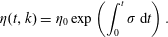 $$\begin{eqnarray}\displaystyle & \displaystyle \unicode[STIX]{x1D702}(t,k)=\unicode[STIX]{x1D702}_{0}\exp \left(\int _{0}^{t}\unicode[STIX]{x1D70E}\,\text{d}t\right). & \displaystyle\end{eqnarray}$$
We perform this integration numerically from
 $t=0$
(at which
 $h=1$
) until the time at which the flow reaches
 $h=L$
. We then find the maximum value of
 $\unicode[STIX]{x1D702}/\unicode[STIX]{x1D702}_{0}$
taken over all wavenumbers. Figure 12(a) shows an example calculation of the maximum (with respect to the wavenumber
 $k$
) amplitude of the perturbation on a
 $\log$
scale, as a function of the distance which the interface has migrated through the channel, starting at the widest point where
 $h=1$
and the RT instability is dominant. Figure 12(b) shows the corresponding evolution of the wavenumber of the mode with maximum amplitude, again as a function of the position in the channel.
As time progresses,
 $h$
decreases, and the magnitude of the maximum disturbance over wavenumber generally increases, as shown in blue for the case
 $Ca=9.3\times 10^{-6}$
and
 $Bo=3.8\times 10^{4}$
. However, for specific parameter values (examples of which are shown in green, corresponding to
 $Ca=6.9\times 10^{-6}$
and
 $Bo=2.8\times 10^{4}$
) it is possible that, while every individual mode is unstable either to a ST or RT instability, the amplitude of the maximum perturbation decreases. This is because the rate at which the perturbation grows is slower than the rate at which the wavenumber of the most unstable mode changes.
For both of the above cases (the blue and green lines), as the interface passes through the channel, the wavenumber of the most unstable mode reaches a minimum because the perturbation surface tension acts most strongly for shorter wavelengths, and so the higher wavenumbers are stabilised more effectively than the smaller wavenumbers: in the region where both ST and RT are weak, surface tension is comparatively strong, and so in this intermediate region of the channel the most unstable wavelength increases.
The red line (for
 $Ca=4.6\times 10^{-6}$
and
 $Bo=1.9\times 10^{4}$
) illustrates a third case where the flow is always stable with respect to the ST instability and is unstable to the RT instability in
 $h>0.92$
. For smaller values of
 $h$
the only instability is the geometric instability, acting on very small-wavenumber disturbances but still leading to significant growth.
8 Oil well application
In the introduction it was mentioned that such an instability may arise in the context of drilling in oil wells, when an oil-based suspension of drilling fluid in the annular region between the well bore and a casing pipe is displaced by cement. In many long-reach wells, the wells are nearly horizontal, and extend several kilometres through the reservoir. Typically, owing to the small curvature of the well along its axis, the casing pipe is not located exactly in the centre of the well bore, and so the cement tends to migrate along the widest part of the annular gap. This can lead to the formation of a laterally extensive interface between the two fluids, analogous to that shown in the experiments of Woods & Mingotti (Reference Woods and Mingotti2016). If the mud is not located above the cement, then this interface will subsequently migrate around the annulus under gravitational forces (e.g. figure 1
b), and, since the gap width varies around the annulus, aspects of the evolution of the interface may be captured by the analysis herein. Although, in general, drilling fluids exhibit non-Newtonian rheology, if we assume the yield strength of the fluids is exceeded and the flow has commenced, then we can assess the values of the control parameters in the present flow. We expect that the mud and cement have viscosities of approximately
 $0.01{-}0.1~\text{Pa}~\text{s}$
, and densities in the range
 $1100{-}1200~\text{kg}~\text{m}^{-3}$
. The flow around the annulus will be driven by the overall pressure gradient associated with the buoyancy, leading to a flow speed of the order of
 $Q=10^{-7}~\text{m}^{3}\text{s}^{-1}$
and a speed of the order of
 $0.001{-}0.1~\text{ms}^{-1}$
.
It follows that, with surface tension
 $0.04~\text{N}~\text{m}^{2}$
and a gradient in gap width of
 $0.001{-}0.01~\text{m}^{-1}~\text{m}$
, we could have
 $\unicode[STIX]{x0394}\unicode[STIX]{x1D70C}g\sim 1000~\text{kg}~\text{m}^{-2}~\text{s}^{-2}$
,
 $2\unicode[STIX]{x1D6FE}\unicode[STIX]{x1D6FC}\cos \unicode[STIX]{x1D703}\sim 10^{-3}~\text{kg}~\text{s}^{-2}$
and
 $12Q\unicode[STIX]{x1D707}_{2}(1-M)\sim 10^{-7}~\text{kg}~\text{ms}^{-2}$
. This would mean that for gap widths
 $b>10^{-3}~\text{m}$
the system would be unstable to a RT instability, for
 $b<10^{-4}~\text{m}$
the system would be unstable to a ST instability, and for intermediate values of
 $b$
the stabilising in-channel surface tension would dominate both the RT and ST instability effects.
9 Conclusion
We have analysed the stability of a fluid–fluid displacement through a thin channel the width of which gradually changes in the direction of flow. Depending on the parameters, we have found that the Saffman–Taylor instability may dominate in the narrow part of the channel where the flow is fastest, while the Rayleigh–Taylor instability may dominate in the widest part of the channel. For intermediate channel widths, the flow may be stabilised by the gradient of the pressure jump across the interface associated with the in-channel surface tension. Corresponding results for the case in which the surface tension is destabilising and the viscosity difference of the fluids across the interface leads to a stabilising effect arise in the case that the effective contact angle
 $\unicode[STIX]{x1D703}-\unicode[STIX]{x1D711}>\unicode[STIX]{x03C0}/2$
and in which
 $\text{sgn}(Q)=1$
. Our results are consistent with the local stability analysis presented by Al-Housseiny et al. (Reference Al-Housseiny, Tsai and Stone2012) but provide new insight into the competition between the stabilising and destabilising processes and their evolution as the flow migrates across the channel.
The evolution of the dispersion relation as an interface migrates across a channel with non-uniform channel width leads to an evolution of the most unstable wavenumber, and in some cases there may be a change in the stability of particular wavenumbers. In particular, owing to the stabilising effect of the in-channel surface tension, there is a shift to larger-wavelength perturbations being of largest amplitude in the centre of the channel, before returning to the smaller wavelengths associated with the ST or RT instabilities in the narrow or wide part of the channel.
Acknowledgement
This work was supported by the BP Institute for Multiphase Flow.