2.1. Data structure for loss reserve

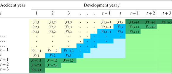
The run-off triangle aligns the claim/loss history of claim/loss size or frequency for a certain type of insurance across accident and development years. The triangular array in yellow colour in Table 1 displays this structure. The entry $y_{i,j}$ are incremental losses in accident year i and development year j where $i,j=1,2, \dots,t$ where t represents current year. Let the set of all observable $T = t(t + 1)/2$ losses in the run-off triangle in calendar year $k=i+j-1\le t$ be the vector

(2.1) \begin{equation} \textbf{y}_{1:T} = \left\{\text{y}_n=y_{i,j}: (i, j) \in \mathcal{I}_{1:t}, \ n=\sum_{r=1}^{i-1} (t-r+1)+j \right\} \end{equation}

that appends rows of the run-off triangle into a vector where $\text{y}_n, n=1, \dots, T$ denotes each loss in $\textbf{y}_{1:T}$ that corresponds to certain $y_{i,j}$ in the run-off triangle and the index sets of losses in calendar year k and in calendar years 1 to t are given respectively by

(2.2) \begin{equation} \mathcal{I}_{k}=\{(i, j)\,{:}\, i + j = k+1 \}\ \mbox{and}\ \mathcal{I}_{1:t} = \bigcup\limits_{k=1}^t \mathcal{I}_{k}. \end{equation}

Table 1.

Layout of incremental loss data with the run-off triangle highlighted in yellow. Unobserved losses within t accident and development years are in blue or otherwise in green. Losses for the future three calendar years are in deep blue and mid to deep green in the trapezoid.

Let $\textbf{y}^c_{k}=\{y_{i,j}: (i, j) \in \mathcal{I}_{k}\}=(\,y_{1,k},y_{2,k-1},\dots, y_{k,1})$ be the vector of losses in calendar year k. Then, the sum of losses for calendar year k is the sum of the k-th diagonal entries

(2.3) \begin{equation} s_k=\sum_{r=1}^k y_{r,k-r+1}, k=t+1, t+2, \dots. \end{equation}

Let $\textbf{y}^p_{t}=\{y_{i,j}: i, j \le t, i+j>t+1\}$ be the vector of non-observable losses in the lower triangle (blue cells of Table 1) and $\textbf{y}^t_{t}=\textbf{y}^p_{t} \cup \{y_{i,j}: i>t \ \mbox{or} \ j > t \ \mbox{or} \ i,j>t\}$ be the vector of all non-observable losses (blue and green cells in Table 1) outside the run-off triangle. The Costa and Pizzinga (Reference Costa and Pizzinga2020) called those losses $y_{i,j},i>t$ or $j>t$ or both (light, mid, and dark green cells) “the tail effects.” Most loss reserve models predict losses in $\textbf{y}^p_{t}$ . Since these losses are within the rectangle, it is easier to predict using observable losses $y_{i,j}, i+j \le t+1$ . However, those tail effect losses are harder to predict because the observable losses do not provide information for future accident, development, and calendar year effects when $i,j>t$ . Costa et al. (Reference Costa, Pizzinga and Atherino2016) and Costa and Pizzinga (Reference Costa and Pizzinga2020) defined three types of reserves:

1. 1. Partial reserve refers to the sum of losses in $\textbf{y}^p_{t}$ (light and dark blue cells in Table 1) in the lower triangle (Renshaw and Verrall, Reference Renshaw and Verrall1998; Chan et al., Reference Chan, Choy and Makov2008; Costa et al., Reference Costa, Pizzinga and Atherino2016).

2. 2. Total reserve represents the sum of losses in $\textbf{y}^t_{t}$ (all blue and green cells) outside the run-off triangle (Atherino et al., Reference Atherino, Pizzinga and Fernandes2010; Costa et al., Reference Costa, Pizzinga and Atherino2016).

3. 3. Calendar year reserve corresponds to the sum of losses in $\textbf{y}^d_{k}$ for calendar year $k >t$ (each lower diagonal of the run-off triangle). These reserves are important for managing short-term financial decisions, as they are the reserves for payments expected to occur soon. Costa et al. (Reference Costa, Pizzinga and Atherino2016) considered one step ahead calendar year reserve forecast.

In this paper, we forecast $h=3$ calendar year reserve $s_{k}, \ k=t+1,t+2,$ $t+3$ . We also provide the popular partial reserve forecast. The calendar year reserve forecasts require losses that are highlighted in dark green ( $i,j=1$ ) and mid green in Table 1 for three future calendar years. Models that capture the trend of effects by the ANCOVA model and the CARR model for development year effect facilitate the forecast of losses beyond year t. For the ANOVA models, we make further assumptions to enable the forecast. Details are provided in Section 3.1.1. As the $h=3$ diagonals of loss forecasts take the shape of a trapezoid, we call these losses the trapezoidal losses.

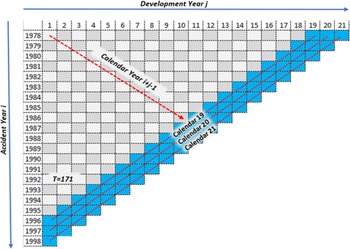
The layout of the data structure in Table 1 is further depicted in Figure 1 for the data we analyse. These data were analysed by Chan et al. (Reference Chan, Choy and Makov2008) and Chan (Reference Chan2015) previously. It contains paid to the insured of an insurance company in Israel during the accident year 1978–1995 and the development year 1–18 with $t=18$ accident, development, and calendar years. There are $T=171$ observations in the upper triangle highlighted in grey. The three calendar year reserves for 1996–1998 are highlighted in the blue trapezoid with red dashed lines.

Figure 1.

Data structure with observed losses in the upper triangle in grey and forecast losses in the trapezoid in blue. The red dashed line indicates the three future calendar years.

2.2. Data features

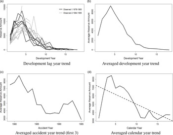
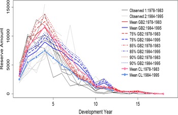
Figure 2 visualises the trend of effects across accident year, development year, and calendar year. For the development year effect, Figure 2(a) shows two distinct quadratic trends: the trend for years 1978–1983 (in black) peaks in the fourth development year and drops gradually thereafter, whereas the trend for years 1984–1995 (in grey) peaks in the sixth development year and drops more gently. Figure 2(b) shows the average of these trends with a sharp peak in the fourth development year. To display the trend of the accident year effect, we note that averaging over development years can be misleading as later accident years do not have the lower losses coming from later development years. A compromise is to plot in Figure 2(c) the trend of accident year losses averaged over the first three development years. For years 1994 and 1995, the averages are based on the first two losses and first loss, respectively. For accident year effect, we observe a general decreasing trend with noises. Lastly, for calendar year effect, Figure 2(d) plots the average of diagonal entities across calendar years. Apart from the first two values with noises, there is a downward trend, showing some linear effect.

Figure 2.

Trends of development, accident, and calendar year effects in the run-off triangle data.

3.1. Proposed statistical models

3.1.1. Mean functions

We model the incremental loss $y_{i,j}$ using different error distributions $\mathcal{D}(\boldsymbol \theta)$ and mean functions $\mu_{i,j}$ as below:

(3.1) \begin{eqnarray}y_{i,j} & = & \mu_{i,j} \epsilon_{i,j}, \epsilon_{i,j} \sim \mathcal{D}(1,\boldsymbol \nu), \ \mbox{E}(\epsilon_{i,j})=1,\end{eqnarray}

where $y_{i,j} \sim \mathcal{D}(\mu_{i,j},\boldsymbol \nu)$ denotes any distribution defined on the positive real support $\mathbb{R}^+$ such as GB2, GG, Weibull, and EE (see Section 3.1.2), $\mbox{E}(\,y_{i,j})=\mu_{i,j}=g(\eta_{i,j})$ , $\eta_{i,j}$ is a linear function of predictors and $\boldsymbol \nu$ is a vector of shape parameters for the distribution. The mean function $\mu_{i,j}$ is defined in three aspects: 1. the type of parameters in $\eta_{i,j}$ ; 2, the functional form of the predictors, for example, in the ANOVA and ANCOVA models; 3. the link function $g(\eta_{i,j})$ that links $\eta_{i,j}$ to $\mu_{i,j}$ .

For the first aspect, the linear function $\eta_{i,j}$ contains four types of parameters: 1. $\alpha_i$ for the accident year effect, 2. $\beta_j$ for the development year effect, 3. $\delta_{i+j-1}$ for the calendar year effect, and 4. $\gamma_{1l}$ for the autoregressive effect and $\gamma_{2l}$ for the persistent effect across development years using the CARR model. We call the model with ANOVA and CARR(p,q) mean function as the ANOVA-CARR(p,q) model. It is defined as:

(3.2) \begin{align} \mu_{i,j}|\boldsymbol{{y}}_{\boldsymbol{{i}},\textbf{1:}(\,\boldsymbol{{j}}-\textbf{1})},\boldsymbol \mu_{i,1:(\,j-1)}&= \eta_{i,j} =\mu_0+\alpha_{i}+\beta_j+\delta _{i+j-1}\nonumber\\[3pt] &\quad +\sum_{l=1}^{p} \gamma_{1l} \, y_{i,j-l} + \sum_{l=1}^{q} \gamma_{2l} \, \mu_{i,j-l}, \end{align}

where the parameter constraints are $\sum_{i=1}^t \alpha_i=\sum_{j=1}^t \beta_j=\sum_{k=1}^t \delta_k=0$ . We assume $y_{i,0}=r_0 y_{i,1}$ and $\mu_{i,0}=0$ where the initial development factor $r_0 \simeq 0.7$ is estimated by the average of $y_{i,1}/y_{i,2}, \ i=1,\dots,17$ . In our studies, we consider only order $(p,q)=(1,1)$ as higher-order effects are often insignificant, and they also need longer development year data to estimate.

For the second aspect, there are three models to specify the predictor effects: the ANOVA, ANCOVA, and mixed ANOVA/ANCOVA models. Predictors in the ANCOVA model can describe the trend patterns using the general additive model $\theta_u=\sum_{l=1}^g w_l f_{l}(u)$ where $\theta_u=\alpha_i,\beta_j,\delta_{i+j-1}$ , $w_l$ is the weight for function $f_{l}(\cdot)$ and g is the number of $f_{l}(\cdot)$ to describe the trend pattern (Verrall, Reference Verrall1996). Although the general additive model can be very general, the trend patterns observed in Figure 2 are not sophisticated but noisy. Hence, we propose the following parsimonious ANCOVA-type predictors:

1. 1. linear accident year effect $\alpha_i =\alpha_s=\alpha \, y_{i1}$ proportional to the first development year loss $y_{i1}$ (denoted by $\alpha_s$ in Table 2),

2. 2. quadratic development year effect $\beta_j=\beta_q=\beta_{1} \, j+\beta_{2}\, j^2$ (denoted by $\beta_q$ ), and

3. 3. linear calendar year effect $\delta_{i+j-1} =\delta \, (i+j-1)$ (denoted by $\delta_l$ ) (Verrall, Reference Verrall1996).

Table 2.

List of mean functions expressed using the symbols in (3.2) and (3.3) in Section 3.1.1.

Note: 1. models in bold face with DIC $<3070$ are selected in Section 5.1; 2. model with has no log transformation.

These terms can replace the corresponding ANOVA-type predictors in (3.2). For the third aspect, the mean function $\mu_{i,j}=g(\eta_{i,j})$ is linked to a linear function of predictors $\eta_{i,j}$ through the link function $g(\cdot)$ . We consider two types of link function: 1. the identity link $\mu_{i,j}=g(\eta_{i,j})=\eta_{i,j}$ in which all location parameters $\mu_0,\alpha_i,\beta_j,\delta_{k},\gamma_{1l},\gamma_{2l}>0$ , for $i,j,k<t$ and $\mu_0$ is adjusted to ensure a positive mean $\mu_{i,j}>0$ for the distributions $\mathcal{D}(\mu_{i,j},\boldsymbol \nu)$ on the positive support and 2. the log link $\log(\mu_{i,j})=\eta_{i,j}$ or $\mu_{i,j}=\exp(\eta_{i,j})$ to describe the non-linear effects of predictors on the mean function. Accordingly, the model in (3.2) becomes

(3.3) \begin{align} \mu_{i,j}|\boldsymbol{{y}}_{\boldsymbol{{i}},\textbf{1:}(\,\boldsymbol{{j}}-\textbf{1})},\boldsymbol \mu_{i,1:(\,j-1)}&=\exp(\eta_{i,j}) =\exp[\mu_0+\alpha_{i}+\beta_j+\delta _{i+j-1}\nonumber\\[3pt]&\quad +\sum_{l=1}^{p} \gamma_{1l} \, \log(\,y_{i,j-l}) + \sum_{l=1}^{q} \gamma_{2l} \, \log(\mu_{i,j-l})], \end{align}

where $\alpha_i, \beta_j, \delta_k$ have no positive constraints.

The models with mean functions (3.2) and (3.3) are used to estimate in-sample losses (yellow cells in Table 1) and forecast out-of-sample losses (blue cells in Table 1). However, for losses outside the observation period with $i,j>t$ (green cells in Table 1), the ANOVA terms $\alpha_i, \beta_j, \delta_k, \, i,j,k>t$ in the mean function $\mu_{i,j}$ are unavailable. We propose to estimate $\hat{\alpha}_i=\hat{\alpha}_t,\, \hat{\beta}_j=\hat{\beta}_t, \hat{\delta}_{k+1}=r_d \hat{\delta}_k, \, i,j,k>t$ . The first assumption is justified by Figure 2(c) showing no clear trend in later accident years. The impact of the second assumption for the development year effect should be minimal as it approaches zero in later development years. The last assumption for the calendar year effect captures the decreasing trend in Figure 2(d) where the ratio $r_d$ can be estimated from the data. For the autoregressive and persistence terms, we set 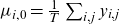$\mu_{i,0}=\frac{1}{T} \sum_{i,j} y_{i,j}$ , $y_{i,0}=r_0 y_{i,1}, i \le t$ and $y_{i,0}=y_{t,0},\, i>t$ again since there is no clear trend for later accident years. The ratio $r_0$ is estimated using $r_0=\frac{1}{17}\sum_{i=1}^{17} \frac{y_{i,1}}{y_{i,2}} \simeq 0.7$ . We also estimate the unobserved $y_{i,j-1},\, i+j>t+2$ as required in the CARR model forecast by simulation, that is, $\hat{y}_{i,j-1} \sim \mathcal{D}(\mu_{i,j-1},\boldsymbol \nu)$ . These assumptions allow reasonable guesses for the unknown parameters using data information. Better ways to estimate these boundary parameters can be adopted if additional information can be obtained from the insurance companies. Details for the four distributions and their shape parameters are provided in the next section.

3.2. Models for comparison

Models including the state-space model in (1.3), the Hoerl curve model in (1.6), and the CSR model in (1.7) attempt to capture the changes in development year pattern across accident years. Among these models, the CSR model (Meyers, Reference Meyers2015) interprets the changes in terms of changing settlement rates and attributes the accelerating claim settlement, for example, due to technological advancement. Our proposed CARR model, on the other hand, uses autoregressive parameter $\gamma_1$ and persistent parameter $\gamma_2$ to describe the development year pattern changes. To facilitate comparison with the CSR model, we assume the losses $y_{i,j}$ in the CSR model given by (3.1) with mean function (1.7) to follow some distributions $\mathcal{D}(\mu_{i,j},\boldsymbol \nu)$ in Section 3.1.2 and call the model GB2-CSR if the CSR model adopts the GB2 distribution.

We also compare our proposed models with the popular CL method based on cumulative claims

\[ z_{i,j}=\sum_{j^{\prime}=1}^{j} y_{i,j^{\prime}},\ \ j=1,\dots, t-i+1,\ \ i=1,\dots, t \]

as the sum of incremental losses from start to current development year. The method first evaluates the lag-to-lag development factor

(3.10) \begin{equation} \varphi_j =\frac{\sum_{i=1}^{t-j+1} z_{i, j}}{\sum_{i=1}^{t-j+1} z_{i,j-1}}, \quad 2\leq j \leq t, \end{equation}

which is the ratio of the sum of cumulative losses over accident years from one development year j to the previous year $j-1$ . Then, it applies the factor $\varphi_j$ to the cumulative loss $z_{i,j-1}$ to estimate the next cumulative loss

\[\hat{z}_{ij}=z_{i,j-1} \times \varphi_j, \quad 2\leq j \leq t-i+1.\]

By assuming constant development factors $\varphi_j$ independent of the accident year i and applying the method recursively to the next cumulative loss, the CL method can be used to estimate cumulative losses

(3.11) \begin{equation} \hat{z}_{ij}=\hat{z}_{i,t-i+1} \times \prod_{j^{\prime}=t-i+2}^{j} \varphi_{j^{\prime}},\quad i=2, ..., t, j>t-i+1 \end{equation}

in the lower triangle as highlighted in blue in Table 1 using the latest observable cumulative losses $\hat{z}_{i,t-i+1}=z_{i,t-i+1}$ for accident year i. However, the method fails to estimate future cumulative losses $z_{i,j}, \ i,j > t$ when the accident or development years are greater than t (in green in Table 1). The problem stems from the unavailability of loss information $z_{i,j}, \ i > t$ for future accident and future development factors $\varphi_{j}, \ j>t$ . To solve the problem, we propose to estimate $z_{t+h, 1},h=1,2,\dots$ and $z_{1, t+h},h=1,2,\dots$ which are highlighted in dark green in Table 1 using other models such as our best-proposed model with additional assumptions. Then, we can estimate $z_{t+h, j}, \ j=2,\dots$ and $z_{i, t+h}, \ i=2,\dots$ using (3.11) replacing t with $t+h$ . Lastly, the estimated incremental losses can be obtained by differencing the two consecutive cumulative losses. This modified CL method is called the trapezoidal CL method.

4.1. Bayesian approach

The fitting of the elaborated loss reserve models in (3.1) and (3.2) via the likelihood approach can be difficult because the density functions such as (3.6) and (3.9) and their derivatives are complicated. We adopt the Bayesian MCMC approach, which has several advantages over the classical likelihood approach.

Firstly, it incorporates both data information $f(\textbf{y}_{1:T} |\boldsymbol{\theta})$ ( $\textbf y_{1:T}$ is defined in (2.1)) and prior information $\pi(\boldsymbol{\theta})$ in estimating the posterior distribution

\[\pi(\boldsymbol{\theta} | \textbf{y}_{1:T} )=\frac{f(\textbf{y}_{1:T} |\boldsymbol{\theta})\ \pi(\boldsymbol{\theta})}{\int f(\textbf{y}_{1:T} | \boldsymbol{\theta})\ \pi(\boldsymbol{\theta}) \ d\boldsymbol{\theta}}\propto f(\textbf{y}_{1:T}| \boldsymbol{\theta})\pi(\boldsymbol{\theta}), \]

where $\boldsymbol \theta=(\boldsymbol \vartheta,\boldsymbol \nu)$ is the vector of all parameters and $\boldsymbol \vartheta$ is the vector of regression parameters. The joint density $f(\textbf{y}_{1:T} |\boldsymbol{\theta})$ is the product of density for each observation $y_{i,j} \in \textbf{y}_{1:T}$ given by (3.6), (35) (in Appendix B), (38) (in Appendix C), and (3.9), respectively, for the four distributions. The mean function $\mu_{i,j}=g(\eta_{i,j})$ where $\eta_{i,j}$ is defined in (3.2) using the vector of regression parameters $\boldsymbol \vartheta$ . The specification of prior information $\pi(\boldsymbol{\theta})$ provides a powerful mechanism to incorporate expert knowledge often available to insurance companies. In the situation where there is a lack of prior information, non-informative or reference priors can be used. The use of non-informative priors leads to objective Bayesian inference (Berger, Reference Berger2006). We use non-informative gamma priors for parameters defined on positive supports and normal priors for unrestricted parameters, both with large variance. These unrestricted parameters refer to the regression parameters in the mean function with log transformation. The hyperparameters are set or tuned to provide large variance and stable posterior distribution.

Secondly, inference for any parameter of interest can be conducted based on the posterior sample without relying on the asymptotic normality assumption in the likelihood approach. This asymptotic normality assumption is often not applicable due to insufficient sample size in real applications. Thirdly, by combining the posterior distributions with the sampling distribution, the entire posterior predictive distribution of future losses can be obtained for reserve forecast.

To illustrate the idea of posterior predictive distribution, we consider forecast of the future h years of losses as an example. These losses $\{y_{i,j}: (i,j) \in \mathcal{I}_{(t+1):(t+h)}\}$ where $\mathcal{I}_{a:b}$ defined in (2.2) are the diagonal entities of the dash lines in Figure 1. The vector of these $M=h(2t+h+1)/2$ losses is written as

(4.1) \begin{align} \textbf{y}_{(T+1):(T+M)}&=(\textbf{y}^d_{t+1},\textbf{y}^d_{t+2},\dots,\textbf{y}^d_{t+h})\nonumber\\[3pt]&=(\,y_{t+1,1},\dots,y_{1,t+1}, y_{t+2,1},\dots,y_{1,t+2},\dots,y_{1,t+h},\dots,y_{t+h,1}) \end{align}

in the order of calendar year (instead of accident year for the in-sample data) to facilitate forecasts by calendar years. Loss forecasts $\text{y}_{T+m}, \, m=1,\dots,M$ are based on the posterior predictive distribution defined as

(4.2) \begin{align}&f(\text{y}_{T+m}|\textbf{y}_{1:T})\nonumber\\[3pt] &\quad = \int \dots \int \prod_{s=1}^{m} \left[ f( \text{y}_{T+s}| \boldsymbol \theta,\textbf{y}_{(T+1):(T+s-1)}, \textbf{y}_{1:T}) \,d\textbf{y}_{(T+1):(T+s-1)} \right] \pi(\boldsymbol \theta|\textbf{y}_{1:T}) d\boldsymbol \theta. \end{align}

The integral over $d\textbf{y}_{(T+1):(T+s-1)}$ is to integrate out the unobserved $\textbf{y}_{(T+1):(T+s-1),}$ whereas the integral over $d\boldsymbol \theta$ is to incorporate prior information. These integrals can be approximated by the Monte Carlo estimator, constructed from the posterior samples according to

(4.3) \begin{eqnarray}& & \hat{f}( \text{y}_{T+m}|\textbf{y}_{1:T}) = \frac{1}{L}\sum_{l=1}^{L} f(\text{y}_{T+m}|\boldsymbol \theta^{(l)},\textbf{y}_{(T+1):(T+m-1)}^{(l)}, \textbf{y}_{1:T}),\end{eqnarray}

where L is the number of iterations after burn-in in each MCMC sampler run given the current window of information, and 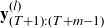$\textbf{y}_{(T+1):(T+m-1)}^{(l)}$ and $\boldsymbol \theta^{(l)}$ are the l-th draw in the posterior sample of $\textbf{y}_{(T+1):(T+m-1)}$ and $\boldsymbol \theta,$ respectively. Essentially, (4.3) implies that the mean forecast $\hat{\text{y}}_{T+m}$ is the mean of the posterior sample

\[\mathcal{S}_{\text{y},T+m}=\left\{\text{y}_{T+m}^{(l)}: \text{y}_{T+m}^{(l)} \sim \mathcal{D}(\mu_{T+m}^{(l)}(\textbf{y}_{(T+1):(T+m-1)}^{(l)},\textbf{y}_{1:T}),\boldsymbol \nu^{(l)}), \, l=1,\dots,L\right\},\]

where the distribution $\mathcal{D}(\cdot)$ has the density $f(\cdot)$ , mean parameter $\mu_{T+m}^{(l)}$ and shape parameters $\boldsymbol \nu^{(l)}$ . The mean parameter is the function $\mu_{T+m}^{(l)}(\textbf{y}_{(T+1):(T+m-1)}^{(l)},\textbf{y}_{1:T})$ defined in (3.2) or (3.3). It depends on simulated observations 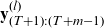$\textbf{y}_{(T+1):(T+m-1)}^{(l)}$ , regression parameters $\boldsymbol \vartheta^{(l)}$ and data $\textbf{y}_{1:T}$ . The vector of all parameters is $\boldsymbol \theta^{(l)}=(\boldsymbol \vartheta^{(l)}, \boldsymbol \nu^{(l)})$ at the l-th draw. The distribution $\mathcal{D}(\cdot)$ is one of the four distributions we consider. The posterior predictive sample $\text{y}_{T+m}^{(l)}$ can be simulated using (32), (36), (39), and (40) (in Appendices A–D), respectively. Apart from the mean forecast, these posterior predictive samples $\mathcal{S}_{\text{y},T+m}$ also provide any u-th ( $u \in (0,1)$ ) level quantile forecast $\hat{\text{y}}_{T+m,u}$ given by the u-th quantile of the posterior sample $\mathcal{S}_{\text{y},T+m}$ . In-sample mean or quantile loss estimates are defined similarly based on the posterior samples $\mathcal{S}_{\text{y},t}, t \le T$ given the data $\textbf{y}_{1:T}$ . Parameter estimates are given by the mean of the posterior samples, that is, 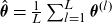$\hat{\boldsymbol \theta}=\frac{1}{L} \sum_{l=1}^L \boldsymbol \theta^{(l)}$ .

Lastly, the models are implemented via the user-friendly Bayesian software Stan which applies the efficient Hamiltonian Monte Carlo (HMC) and No-U-Turn samplers (Hoffman and Gelman, Reference Hoffman and Gelman2014). RStan (Carpenter et al., Reference Carpenter, Gelman, Hoffman, Lee, Goodrich, Betancourt, Brubaker, Guo, Li and Riddell2017) utilises the Stan program within R developed in the C++ language. The HMC sampler (Duane et al., Reference Duane, Kennedy, Pendleton and Roweth1987; Neal, Reference Neal1994) as a class of MCMC sampling methods converges faster than the conventional samplers such as random-walk Metropolis (Metropolis et al., Reference Metropolis, Rosenbluth, Rosenbluth, Teller and Teller1953) and Gibbs sampler (Geman and Geman, Reference Geman and Geman1984) for some complicated models with many parameters. See also Taylor (Reference Taylor2012), Meyers (Reference Meyers2015), Venter et al. (Reference Venter, Gutkovich and Gao2017), Venter (Reference Venter2018), and Venter and Sahin (Reference Venter and Sahin2018) for more prominent contributions of Bayesian MCMC to the actuarial literature.

4.2. Convergence diagnostics

It is salient to ensure the convergence and independence of the MCMCs. To check these two conditions, graphical plots and numerical measures can be applied. The autocorrelation function (ACF) plot visualises the autocorrelation for each parameter. If an MCMC is dependent, it should decrease quickly with increasing lag. Hence, a positive long-lagged ACF indicates high autocorrelation. To reduce the autocorrelation, Annis et al. (Reference Annis, Miller and Palmeri2017) suggested running longer chains and drawing subsamples from the longer chains. However, if these procedures do not decrease the ACF, the model may be unstable (Vehtari et al., Reference Vehtari, Gelman, Simpson, Carpenter and Bürkner2021). A negative ACF, on the other hand, indicates antithetic Markov chains. To avoid his problem, one can increase the number of chains. Another graphical plot is the traceplot (within the Rstan package). A fuzzy-caterpillar-look trace plot indicates convergence and independence of the MCMC (Lee and Wagenmakers, Reference Lee and Wagenmakers2014).

To evaluate the extent of convergence, we report two measures. The first measure is the number of effective samples $n_{\rm eff}$ after allowing for the dependency in the Monte Carlo sample. Samples that display positive autocorrelation often give smaller $n_{\rm eff}$ . On the other hand, those with negative autocorrelation have larger $n_{\rm eff}$ . We expect $n_{\rm eff}$ to be sufficiently large, such as at least 2000. The second measure proposed by Gelman and Rubin (Reference Gelman and Rubin1992) is a scale reduction measure called $\widehat{R}$ . It is the ratio of the variance of a parameter when the data are pooled across all of the chains to the variance within a chain. The criterion used for convergence is $\widehat{R}$ within $1 \pm 0.0001$ for each parameter. More information for the two criteria can be found in Peters et al. (Reference Peters, Wüthrich and Shevchenko2010).

We carefully inspect the ACF and trace plots for each model parameter. When the two criteria, namely $n_{\rm eff}\ge 2000$ and $\widehat{R} \in 1 \pm 0.0001$ , are not met (confirmed by the ACF and trace plots), we increase the Monte Carlo sample size (iter), including burn-in, gradually. Depending on model complexity, the sample size is chosen from 5000 to 60,000 per chain including the burn-in of 5000 iterations per chain, and we use four chains.

4.3. Model performance measures

Model selection is based on two model performance measures. The DIC consists of two components:

\[\mbox{DIC}=\bar{D}+p_{D} \]

which measures the model fit and penalises model complexity, respectively. The first component is defined as the posterior expectation of the deviance

\[\bar{D}=E_{\theta|\text{y}}[D(\boldsymbol \theta)]=E_{\theta| \text{y}}[-2\ln f(\textbf{y}|\boldsymbol \theta)],\]

where the deviance is $-2$ times the log-likelihood and the second component evaluates the effective number of parameters defined as the difference between the posterior mean of the deviance and the deviance evaluated at the posterior mean $\bar{\boldsymbol \theta}$ of the parameters:

\begin{align*}p_{D}&=\bar{D}-D(\bar{\boldsymbol \theta})=E_{\theta|\text{y}}[-2\ln f(\textbf{y}|\boldsymbol \theta)]+2\ln f(\textbf{y}|\bar{\boldsymbol \theta}).\end{align*}

The posterior expectation is estimated based on the posterior sample of the MCMC output.

The predictive performance of the models is also assessed by comparing the observed losses with the predicted losses using the mean squared error (MSE)

\[ \mbox{MSE}= \frac{1}{T} \sum_{i=1}^t \sum_{j=1}^i \left(\,y_{i,j}-\hat{y}_{i,j} \right)^2, \]

where $\hat{y}_{i,j}=\mu_{i,j}$ in (3.2) or (3.3) for mean estimate and $\hat{y}_{i,j}=\hat{y}_{i,j,u}, \, u \in (0,1)$ where $y_{i,j,u}$ is the u-th quantile of $y_{i,j}$ . In summary, DIC provides adjusted model fit allowing for model complexity whereas MSE assesses prediction accuracy which is more important in loss reserving.

5.1. Model selection

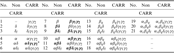
Our data analysis begins with searching for some efficient mean functions adopting the most flexible $\mbox{GB2}$ error distribution. Table 2 shows 41 mean functions we consider. These functions are arranged in two panels (with and without persistence), each with 21 mean functions of accident (A), development (D), and calendar (C) year effects. The 21 mean functions, in seven groups of three each, are identified by a list of parameter symbols (see Section 3.1.1) which indicates the type of parameters included in the mean function. The three members of each group are none, C-ANOVA ( $\delta$ ), and C-ANCOVA ( $\delta_l$ ), showing the exclusion of calendar year effect, inclusion of ANOVA-type calendar year effect, and inclusion of ANCOVA type calendar year effect, respectively. Then, the seven groups correspond to the exclusion or inclusion of the accident and development year effects, namely none, A-ANOVA ( $\alpha$ ), D-ANOVA ( $\beta$ ), AD-ANOVA ( $\alpha\beta$ ), D-ANCOVA ( $\beta_q$ ), A-ANOVA-D-ANCOVA ( $\alpha\beta_q$ ), and AD-ANCOVA ( $\alpha_s\beta_q$ ). We represent the mean function using these symbols and write, for example, GB2- $\alpha\beta$ to represent the model with parameters $\alpha_i$ and $\beta_j$ in the mean function and GB2 as the data distribution.

In fitting these 41 mean functions with the most flexible GB2 distribution, we find the log-transformed mean functions provide consistently better model fit with lower DIC (<3070) except the mean function $\alpha\delta\gamma_1\gamma_2$ . Hence, the mean functions in (3.2) without log transformation are indicated by “ $^*$ ”. We remark that some of these models do not converge or have poor model fits. We report, in Table 3, the model performance measures DIC and MSE for the best GB2- $\beta\delta_l$ model according to DIC. In this model, the calendar year effect replaces the accident year effect possibly because the former displays a clearer linear trend in Figure 2. We also report the GB2- $\beta\delta_l\gamma_1\gamma_2$ model with additional development year persistence effect as it provides the lowest MSE. We repeat this search for the best mean functions with GG, Weibull, and EE distributions. The results are also reported in Table 3. We rank the eight models according to DIC and MSE. Results show that, in general, models with the persistence effect are more likely to provide better in-sample estimates according to MSE. Across distributions, GB2 and GG provide the best model performance. Weibull is slightly worse and EE is the worst.

Table 3.

Performance measures and ranks in bracket for the best fitted model of each distribution without and with development year persistence as well as for the GB2-CSR model.

Note: 1. models in bold face are the best according to DIC & MSE; 2. model with $^*$ has no log transformation.

Previously, Nadarajah and Haghighi (Reference Nadarajah and Haghighi2011) and AbuJarad and Khan (Reference AbuJarad and Khan2018) recommended EE distribution. The former preferred EE among the three distributions, Gamma, Weibull, and the Exponentiated Exponential in Bayesian inference. AbuJarad and Khan (Reference AbuJarad and Khan2018) suggested EE contrasting with exponential and exponentiated exponential distributions for running Stan. However, our experience with this data set shows that EE- $\beta\gamma_1\gamma_2$ model provides in-sample estimates with very high MSE. According to the sum of ranks, the GB2- $\beta\delta_l\gamma_1\gamma_2$ model provides the best overall fit. This model is selected because it provides the most accurate in-sample estimates. We also apply the CSR model in (1.7) and the CL method in Section 3.2 for comparison.

Comparing CARR models with the GB2-CSR model adopting the best GB2 distribution, Table 3 shows that GB2-CSR model performs the worst according to $\mbox{DIC}$ and $\mbox{MSE}$ . One possible reason is that the CARR models adopt a more relaxed assumption on the development year pattern change across accident years which is driven by persistence across development years in the form $\gamma_1 \log(\,y_{i,j-1})+\gamma_2 \log(\mu_{i,j-1})$ using parameters $\gamma_1$ and $\gamma_2$ . Essentially, it uses the previous claim information to forecast claims in the next development year based on development year persistence. This assumed pattern is more data-driven. So, it is different from the explicit pattern $\beta_j (1-\omega)^{(i-1)}$ based on parameter $\omega$ in the CSR model making the CARR model more adaptive to different data. For the CSR model, an increase (decrease) in payment rate during the earlier development period will cause more (less) payments as the accident year increases. However, the converse is not always true as other hidden factors can give rise to the observed phenomenon. Nevertheless, a slowdown in claim settlement is found in our loss data because $\omega$ is estimated to be significantly positive ( $0.0133$ ), in agreement with Figure 2(a) showing slower claim increment for later accident years. Perhaps the technological advancement may not yet affect the settlement rate during the data period of 1978–1995.

The estimation accuracy using the GB2- $\beta\delta_l\gamma_1\gamma_2$ model can be visualised by comparing the observed and estimated losses in Figure 3. The estimated losses are provided at the mean and 75%, 85%, and 90% quantiles. These losses are indicated by red and blue lines respectively for the earlier (1978–1983) and later (1984–1995) accident year periods with two different observed development year patterns as shown in Figure 2(a). The earlier accident years show a sharper and earlier rise and drop of claims across development years than the later accident years. Although the mean function with one common development year ANOVA model ( $\beta$ ) does not differentiate effects between these two periods, the estimated mean and quantile lines capture well the slower decay trend in the later period. The CL method tends to provide underestimates which do not differentiate between the two periods.

Figure 3.

Observed and estimated losses using the mean and quantile estimates of the $\beta\delta_l\gamma_1\gamma_2$ -GB2 model as well as the CL method.

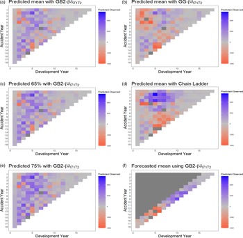
To further visualise the estimation/prediction accuracy, Figure 4 provides the heat maps to distinguish over and underestimation of losses by plotting the differences between estimated and observed losses. The slower rise in the fitted mean in Figure 3 gives more under-fits (red) in early development year (1–4) and more over-fits in later development year (5–8) for earlier accident years than later accident years in Figure 4(a). Figure 4(a) and (b) also show that GG distribution tends to provide more underestimates (in red) which can be hazardous to insurance companies, whereas GB2 distribution provides more accurate losses (in grey). Figure 4(c), (e), and (d) display the accuracy for the 65% quantile of GB2- $\beta\delta_l\gamma_1,\gamma_2$ model, 75% quantile of GB2- $\beta\delta_l\gamma_1,\gamma_2$ model, and the CL method, respectively. It is clear that the quantile estimates show some overestimation. However, the CL method displays both heavier over and underestimation, indicating lower accuracy. Figure 4(f) depicts out-of-sample forecasts which will be discussed in Section 6.3.3.

Figure 4.

Differences between predicted and observed losses in (a) and (b) for comparing between GB2 and GG distributions using the GB2- $\beta\delta_l \gamma_1 \gamma_2$ model; in (c), (e), and (d) for comparing between 65%, 75% quantile of the GB2- $\beta\delta_l \gamma_1 \gamma_2$ model and CL method; and in (f) for validating the out-of-sample forecast using the GB2- $\beta\delta_l \gamma_1 \gamma_2$ model fitted to data with $t \le 15$ .

5.2. Simulation experiments

5.2.1. Validating parameter accuracy

It is challenging to evaluate the accuracy of the parameter estimates from the Stan program in R as the true values are unknown. In this situation, researchers often conduct simulation experiments. Based on the best GB2- $\beta\delta_l\gamma_1\gamma_2$ model, we start by simulating many run-off triangles, each with $T=171$ observations (yellow cells in Table 1), using the parameter estimates as the true values. Then, we fit the GB2- $\beta\delta_l\gamma_1\gamma_2$ model to each simulated data set. If a data set gives one or more cases of $n_{\rm eff}<1000$ , $\widehat{R} \notin 1 \pm 0.001$ or $\mbox{DIC}>3080$ , the model is considered unstable. We will then replace the data with another simulated data and refit the model. We continue the procedures until we obtain $S=100$ sets of parameter estimates.

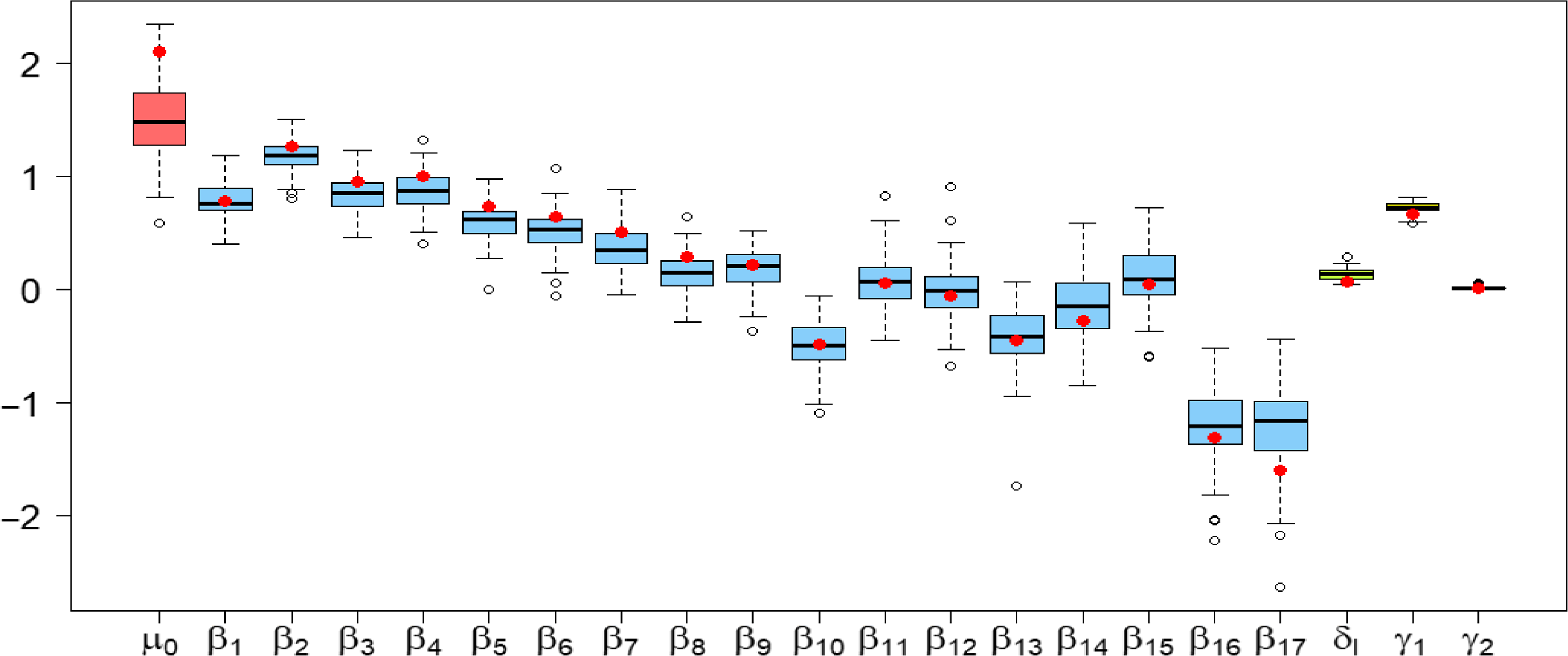
Figure 5 displays the boxplots of 100 estimates for 21 regression parameters, coloured according to the type of regression parameters. We focus on regression parameters in the figure because our experience shows that the mean and quantile estimates are less sensitive to the shape parameters. On inspecting these boxplots, it is not surprising that parameters $\delta_l$ , $\gamma_1$ , and $\gamma_2$ display higher precision than parameters $\beta_j$ because the calendar year effect is clearly linear. Also, there are more observations to estimate the development year persistence $\gamma_1$ and $\gamma_2$ than $\beta_j$ . 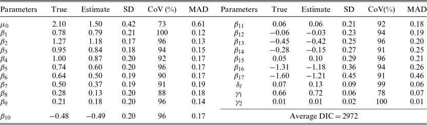Moreover, the precision of $\beta_j$ decreases with j with fewer observations. Table 4 reports the average and standard deviation (SD) for these 100 estimates of each regression parameter. The SDs of $\delta_l$ , $\gamma_k$ , and $\beta_j$ reflect their precision observed in Figure 5. To assess the accuracy for each parameter, we report two measures. The first measure is the mean absolute deviation (MAD) defined for parameter $\theta$ as

\[ \mbox{MAD}(\theta)= \frac{1}{S} \sum_{r=1}^S |\hat \theta_{r}-\theta_{\rm 0}|,\]

where $\theta_{\rm 0}$ denotes the true parameter value and $\hat \theta_r$ is the estimate for the r-th simulated data. The second measure called coverage (CoV) reports the proportion of the 95% credible intervals that cover the true parameter. The CoV measure is defined as

\[ \mbox{CoV}(\theta) = \frac{1}{S} \sum_{r=1}^S I\left(\theta_{\rm 0} \in \left(\hat \theta_{r,0.025}, \hat \theta_{r,0.975}\right)\right) \times 100, \]

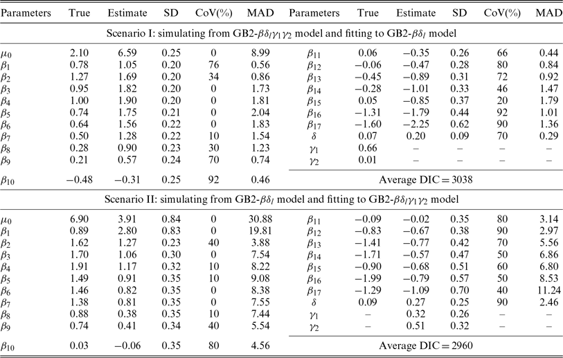
where $\hat \theta_{r,u}$ is the $u \in (0,1)$ quantile in the posterior sample of $\theta$ for the r-th simulated data and I(E) is the indicator function for an event E. The accuracy of the estimates is reasonable for all parameters according to MAD and CoV. Moreover, the DIC averaged over 100 simulations is 2972. This value is close to 3007 in the real data analysis. In summary, parameter estimates using Stan program are reliable.

Figure 5.

Boxplots of 100 estimates for 21 regression parameters with true values indicated by red dots.

Table 4.

True parameter values, estimates, standard deviation, coverage percentage, and MAD of in-sample fit using GB2- $\beta\delta_l\gamma_1\gamma_2$ model with $T=171$ observations and $S=100$ simulated data sets.

5.2.2. Validating CARR model robustness

In this simulation study, we vary the data generating process so that some effects in (3.3) are switched on and off to compare the robustness of models to different data generating processes. To investigate the robustness of the CARR model, we consider models GB2- $\beta\delta_l\gamma_1\gamma_2$ (model A) and GB2- $\beta\delta_l$ (model B). We simulate data from one model and fit it to the other using parameter estimates as true values. We obtain $S=100$ sets of parameter estimates with DIC $<3080$ by simulating around 300 sets for Scenario I (from A to B) and 150 sets for Scenario II (from B to A). Results are reported in Table 5. We note that $\hat \mu_0$ is higher for Scenario I but lower for Scenario II due to the non-inclusion and inclusion of persistence effect $\gamma_1,\gamma_2$ in the fitted model. Inclusion of persistence effect can partially account for the claim level so that $\hat \mu_0$ can be lower. These biases affect the accuracy of the first few $\beta_j$ related to high claim levels. Moreover, the average DIC is 3038 for Scenario I and 2960 for Scenario II, showing the relative advantage in robustness for the in-sample fit of the CARR model even when the data do not display development year persistence. Results for calendar year reserve forecasts are presented in Section 6.3.3. We remark that the DIC of 2960 is also close to the DIC of 3007 in Table 3 for the loss data.

Table 5.

True parameter values, estimates, standard deviation, coverage percentage, and MAD of in-sample fit for each scenario with $T=171$ observations and $S=100$ simulated data sets.

6.1. Partial and calendar year reserve forecasts

Given the in-sample data $\textbf{y}_{1:T}$ , the posterior samples of parameters $\boldsymbol \theta^{(l)}$ and the forecasts 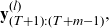$\textbf{y}_{(T+1):(T+m-1)}^{(l)},$ $l=1, \dots, L$ where L is the posterior sample size, the posterior samples of the means 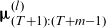$\mathbf{\unicode{x03BC}}_{(T+1):(T+m-1)}^{(l)}$ and the next mean $\mathbf{\unicode{x03BC}}_{(T+m)}^{(l)}$ can be calculated using the mean functions in (3.2) and (3.3).

Then the posterior predictive distribution in (4.3) for the next loss $\text{y}_{T+m}$ is given by

(6.1) \begin{equation} \hat{f}\left(\text{y}_{T+m}|\textbf{y}_{(T+1):(T+m-1)}^{(l)}, \boldsymbol \theta^{(l)},\textbf{y}_{1:T}\right)=\hat{f}\left(\text{y}_{T+m}|\unicode{x03BC}_{T+m}^{(l)},\boldsymbol \theta^{(l)}\right). \end{equation}

Then, the posterior sample of $\text{y}_{T+m}^{(l)},l=1, \dots,L$ can be obtained from simulation, that is, $ \text{y}_{T+m}^{(l)} \sim \hat{f}(\text{y}_{T+m}|\unicode{x03BC}_{T+m}^{(l)},\boldsymbol \theta^{(l)})$ . The mean of these posterior samples of forecasts at various cells is reported in Table 6. The sum of deep and light blue loss forecasts in the lower run-off triangle provides the partial reserve forecast of 223,905 using the GB2- $\beta\delta_l\gamma_1\gamma_2$ model.

We also provide $h=3$ future calendar year loss forecasts $s_{t+1},\dots, s_{t+h}$ in (2.3). These sums of future losses per calendar year include future losses denoted by $\text{y}_{T+m}, \, m=1,\dots, M$ where $M=h(2t+h+1)/2$ . The vector of these losses is denoted by $\textbf{y}_{(T+1):(T+M)}$ and defined in (4.1). The posterior predictive samples $\mathcal{S}_{t+k}=\left\{s_{t+k}^{(l)}, \, l=1,\dots, L\right\}, \, k=1,\dots,h$ of the sum of future loss forecasts by calendar years can be obtained by summing the future losses $\text{y}_{T+m}^{(l)}$ in the posterior predictive sample in calendar year $t+k$ given by

(6.2) \begin{equation} s_{t+k}^{(l)}=\sum_{r=1}^{t+k} y_{r,t+k-r+1}^{(l)}=\sum_{m\,{=}\,(k-1)t+(k-1)k/2+1}^{kt+k(k+1)/2} \text{y}_{T+m}^{(l)}. \end{equation}

Similarly, the mean and quantiles of the posterior predictive samples $\mathcal{S}_{t+k}, k=1,\dots,h$ can be obtained for forecasting.

Table 6.

Mean forecasts using GB2- $\beta\delta_l\gamma_1\gamma_2$ for calendar year reserves (deep blue and green highlights) and partial reserve (lower run-off triangle in deep and light blue highlights).

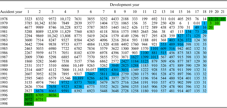
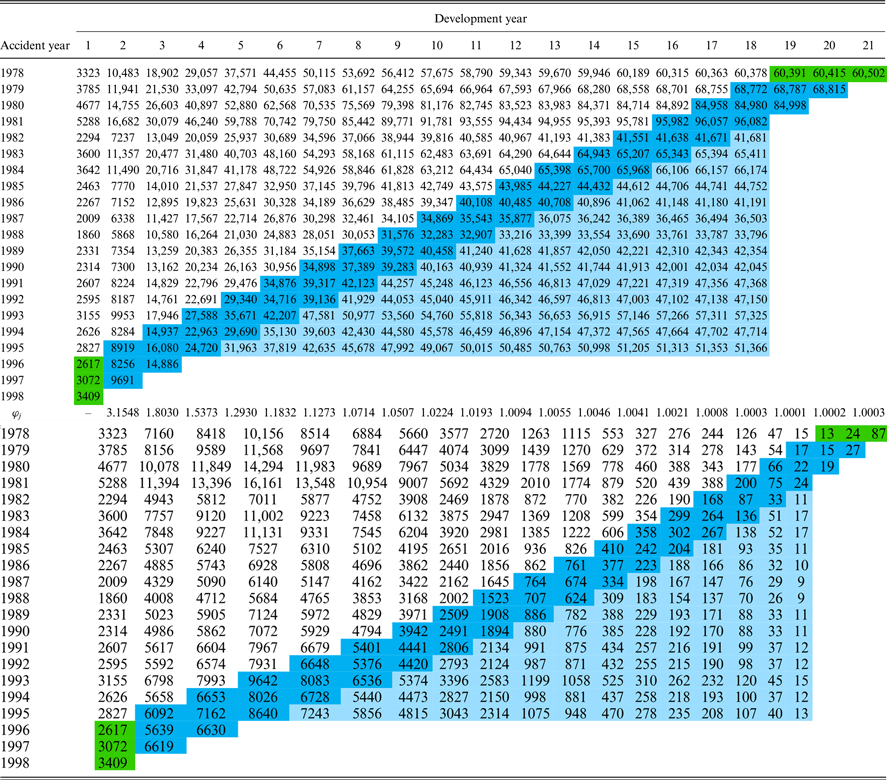
Forecasts using the trapezoidal CL method are also provided for comparison. The observed cumulative (upper panel) and incremental (lower panel) losses and forecasts (in blue and green cells) are reported in Table 7. The upper panel also reports the development factors $\varphi_j$ defined in (3.10) in Section 3.2. These factors show fast increases in earlier development years, slower increases in the middle (after the peak of incremental losses), and near-zero increases near the end. 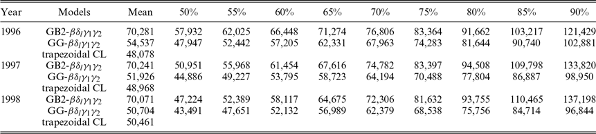The incremental losses in the first row and first column of the lower panel in green cells are estimated using the best GB2- $\beta\delta_l\gamma_1\gamma_2$ model. The mean and quantile calendar year reserve forecasts are reported in Table 8 for the GB2- $\beta\delta_l\gamma_1\gamma_2$ model, GG- $\beta\delta_l\gamma_1\gamma_2$ model, and trapezoidal CL method. The partial reserve forecast is estimated to be 206,383 using the CL method, with individual loss estimates reported in Table 7(b). This partial reserve forecast is lower than 223,905 using the GB2- $\beta\delta_l\gamma_1\gamma_2$ model with individual loss estimates reported in Table 6.

Table 7.

Upper panel: (a) Observed and forecasted (in blue and green highlights) cumulative losses using CL trapezoid method; Lower panel: (b) Observed and forecasted (in blue and green highlights) incremental losses based on the cumulative losses.

Table 8.

Calender year reserve forecast for years 1996, 1997 and 1998.

6.2. Comparing calendar year reserve forecasts

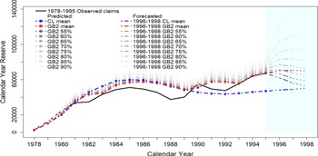
Results of the calendar year reserve forecasts in Table 8 show that the GB2 distribution provides higher forecasts than the GG distribution for all the mean and quantile estimates of all calendar years. The trapezoidal CL method provides the lowest forecasts. Across calendar years, forecasts using GB2 distribution tend to drop for quantiles less than 75%, stabilise for mean and increase for quantiles greater than 80%. These trends drop consistently for GG distribution and trapezoidal CL method. Figure 6 visualises these trends of calendar year reserve by graphing the observed (black line), estimated/forecasted mean (red line), and estimated/forecasted quantiles (grey lines) using the GB2- $\beta\delta_l\gamma_1\gamma_2$ model and the trapezoidal CL method (blue line). The forecast period is highlighted with a light blue background. All calendar year reserve forecasts follow some quadratic trends from 1978 to 1989. These quadratic trends tend to move above the observed calendar year losses from 1981. The red (mean) and grey (quantiles) lines using the GB2- $\beta\delta_l\gamma_1\gamma_2$ model tend to converge to the observed calendar year loss in 1990 and move up closely together. On the other hand, the blue line using the trapezoidal CL method tends to stabilise below the observed calendar year losses from 1990. These underestimates using the trapezoidal CL method can be seen in Figure 3 and confirmed by the MSE of 4800 thousands using the trapezoidal CL method compared to 2671 thousands using the GB2- $\beta\delta_l\gamma_1\gamma_2$ model. The heat map in Figure 4(d) for the trapezoidal CL method also shows more deep red cells (underestimates) in the diagonals. Moreover, the trends of the red and grey lines in Figure 6 display clear lag-1 effects when adopting the development year persistence effect in the model. In summary, the GB2- $\beta\delta_l\gamma_1\gamma_2$ model provides more accurate in-sample estimates of calendar year loss than the trapezoidal CL method.

Figure 6.

Observed, predicted, and forecasted of calendar year reserves at (a) the mean (red line) and quantiles (grey lines) using the GB2- $\beta\delta_l\gamma_1\gamma_2$ model; and (b) the mean (blue line) using the CL trapezoid method.

During the forecast period from 1995 to 1998, the red and grey lines continue to rise gradually in 1996 but start to stabilise in 1997 and 1998 except the quantiles higher than 80%. For the trapezoidal CL method, the blue line shows a mild upward trend. We remark that the quantile lines diverge due to the increase in forecast variability across the forecast period. The variability of calendar year reserve forecast should increase with calendar year k as the posterior predictive sample $\text{y}_{T+m}^{(l)}$ in (6.1) depends on more posterior predictive samples $\textbf{y}_{(T+1):(T+m-1)}^{(l)}$ , adding more sampling variability to $\text{y}_{T+m}^{(l)}$ and hence the calendar year reserve forecast $s_{t+k}^{(l)}$ in (6.2). Moreover, uncertainty also increases in the later accident years with less observed losses and in the later development years with more noises or irregularities. These factors add to the variability of calendar year reserve forecasts. Hence, we expect the flexible $\mbox{GB2}$ distribution can capture these heterogeneities and provide more reliable forecasts. To testify to its flexibility to provide more reliable forecasts, we explore the properties of GB2 distribution in the next section. We also study the amount of over and under-reserve and perform experiments to validate the calendar year reserve forecasts.

6.3. Forecast performance studies

6.3.1. Flexibility of GB2 distribution

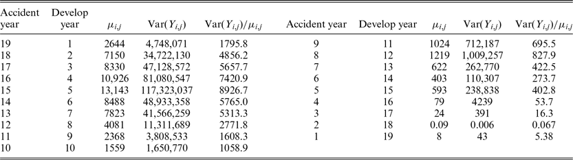
Heterogeneity is often encountered in insurance data. It frequently results in distributions with thick tails. GB2 distribution provides flexible variance to mean ratio compared with the over-dispersed Poisson CL model with a constant variance to mean ratio across cells. Table 9 reports estimates of $\mu_{i,j}$ , $\mbox{Var}(Y_{i,j})$ according to (3.5) and the variance to mean ratio $\mbox{Var}(Y_{i,j})/\mu_{i,j}$ across losses in the first forecasted calendar year 1996. Results show large variabilities in the variance and variance to mean ratio. This ratio is closely related to the mean level across development years. Results show that GB2 distribution allows larger variance to mean ratio when the mean level increases. Hence, it provides extra flexibility to model loss data.

Table 9.

Mean, variance and variance to mean ratio using GB2- $\beta\delta_l\gamma_1\gamma_2$ model for calendar year 1996.

We also compare the flexibility of GB2 distribution with GG distribution within the family to address the discrepancy in calendar year reserve forecasts using the GB2- $\beta\delta_l\gamma_1\gamma_2$ and GG- $\beta\delta_l\gamma_1\gamma_2$ models in Table 8. Cummins et al. (Reference Cummins, Dionne, McDonald and Pritchett1990) stated that GB2 distribution arises from the structural GG $(\,y; a, \theta, p)$ distribution where the scale parameter $\theta$ is distributed as GG $(\theta; - a, b, q)$ . 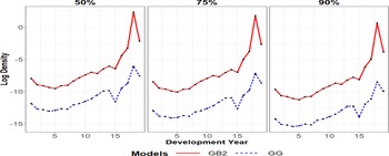Being a scale mixture of GG distributions, GB2 distribution possesses extra heterogeneity relative to the GG distribution. The limiting case when q tends to infinity which signifies GG distribution corresponds to homogeneity. See also Appendix E which explains the difference between the two distributions in terms of Gamma generating distributions. The three shape parameters a, p, and q for GB2 distribution are estimated to be 8.44, 0.22, and 0.34, respectively, whereas a and p for GG distribution are 4.20 and 0.33, respectively. Hence, part of the difference between the two distributions come from q being 0.34 and $\infty$ , respectively. Parameter a is lower in GG distribution to compensate for the thin tail from large q. To testify to this, we compare the log of densities in (3.4) and (33) in Appendix B for the two distributions at three quantiles for each loss in the calendar year 1996. See Appendix F for the calculations. Figure 7 plots the log densities at 50%, 75%, and 90% quantiles across development years. The plots show consistently higher log density for GB2 relative to GG distribution, indicating thicker tails for GB2 distributions. These results explain the lower forecasts using GG distributions since their tails are not thick enough to accommodate extreme losses. In summary, the tail property is an important consideration in choosing loss distribution.

Figure 7.

Log density across development years for calendar year 1996 at 50%, 75%, and 90% quantiles using GB2- $\beta\delta_l\gamma_1\gamma_2$ and GG- $\beta\delta_l\gamma_1\gamma_2$ models.

6.3.2. Under and over loss reserve

Over- and under-reserves for the calendar year reserve forecasts have different implications for insurance companies. Over-reserved during prosperous financial years may not materially impact the company’s current financial condition. However, it reduces the profit and leads to low surplus levels during lean years (Zhang and Browne, Reference Zhang and Browne2013). This incident is viewed in the insurance industry as a dangerous complacency. On the other hand, under-reserving may expose the company to the risk of a shortfall in outstanding liabilities and potential bankruptcy. The amount of over- and under-estimations of individual losses is graphed in Figure 4(a)–(e) for various types of estimates.

McKenzie (Reference McKenzie2011) and De Myttenaere et al. (Reference De Myttenaere, Golden, Le Grand and Rossi2016) proposed to measure the amount of over- and under-reserve using the mean absolute percentage error (MAPE) defined as

(6.3) \begin{equation} \mbox{MAPE}= \frac{1}{t}\sum_{k=1}^t \frac{|\hat s_k-s_k|}{s_k} \times 100, \end{equation}

where t denotes the current year and $\hat{s}_k$ is the estimate of $s_k$ defined in (2.3). Anderson (Reference Anderson1971) suggested that the percentage error for a loss reserve that falls within five percent of the actual loss is reasonable from an actuarial point of view. We adopt an asymmetric criterion of within $-5$ to 15% accepting more over-reserve than under-reserve because under-reserve is more hazardous to an insurance company. To assess the level of over- ( $\hat{s}_k>1.15s_k$ ), acceptable ( $0.95 s_k \le \hat{s}_k \le 1.15 s_k$ ) and under-( $\hat{s}_k<0.95s_k$ ) reserves, we generalise the MAPE measure in (6.3) to the three cases and define

(6.4) \begin{equation} \mbox{MAPE}_g= \frac{1}{t_g}\sum_{k=1}^t I_{k,g} \frac{|\hat s_k-s_k|}{s_k} \times 100, g=+,0,-, \end{equation}

where $I_{k,+}=I(\hat{s}_k>1.15s_k)$ , $I_{k,0}=I(0.95 s_k\le \hat{s}_k \le 1.15 {s}_k)$ , $I_{k,-}=I(\hat{s}_k<0.95s_k)$ and the counts $t_g=\sum_{k=1}^t I_{k,g}, \, g=+, 0, -$ .

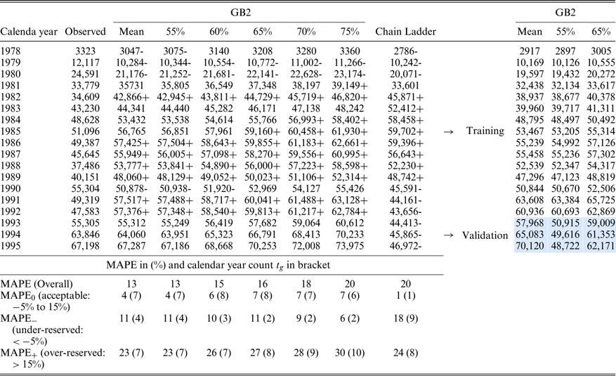
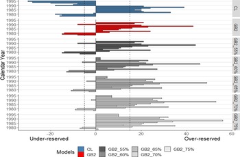
The top left panel of Table 10 reports the calendar year reserve forecast $s_k$ , indicated with “ $+$ ” if it is an over-reserve and “ $-$ ” if it is an under-reserve. The bottom left panel reports $\mbox{MAPE}, \mbox{MAPE}_0$ , $\mbox{MAPE}_-, \mbox{MAPE}_+$ , and the counts $t_g$ in a bracket using the GB2- $\beta\delta_l\gamma_1\gamma_2$ model and the trapezoidal CL method. It is reasonable to see the percentage of under-reserves ( $\mathrm{MAPE}_-$ ) drops, and the percentage of over-reserves ( $\mathrm{MAPE}_+$ ) increases with quantile levels. Comparing the loss reserves using the mean of GB2- $\beta\delta_l\gamma_1\gamma_2$ model and the trapezoidal CL method, the former perform better by having lower MAPE, $\mathrm{MAPE}_-,$ and $\mathrm{MAPE}_+$ with reasonable numbers of counts. Comparing the loss reserves using the mean and quantiles of the $\mbox{GB2}-\beta\delta_l\gamma_1\gamma_2$ model, the loss reserve using the mean estimates is marginally better than the reserve using the 55% quantile estimates. These 55% quantile estimates provide, in term, the best loss reserve among other quantile estimates.

Table 10.

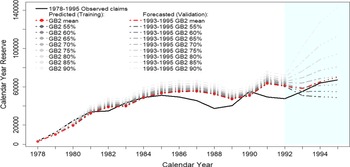
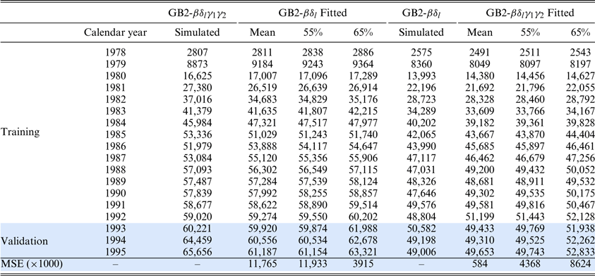
Top left: (a) Observed, estimated, and forecasted calendar year loss using the mean and quantiles of the GB2- $\beta\delta_l\gamma_1\gamma_2$ model as well as using the trapezoidal CL method; Top right: (b) Estimated and forecasted calendar year loss using training data of years 1978–1992; Bottom left: MAPE in percentage with year count in bracket.

Figure 8 plots the percentages of under- (< $-5$ %) and over-reserves (>15%) indicated by two dash lines at $-5$ % and 15%, respectively, for all estimators in all calendar years. The trapezoidal CL method has substantially more under-reserve than the reserves using the $\mbox{GB2}-\beta\delta_l\gamma_1\gamma_2$ model. The amount of over-reserves is relatively similar to the reserves using the mean estimates of the $\mbox{GB2}-\beta\delta_l\gamma_1\gamma_2$ model. As the quantile level rises, it is clear that the amount of under-reserves drops at the cost of increasing over-reserves. Between the reserves using the mean estimates and 55% quantile estimates, the former are slightly better as confirmed in Figure 8.

Figure 8.

Percentages of under- and over-reserves across types of estimators and calendar years.

6.3.3. Validation using 1978–1992 losses

To assess the accuracy of these calendar year reserve forecasts, we conduct two experiments that begin by dividing the data into a training set with losses in 1978–1992 and a validation set with losses in 1993–1995. We fit the GB2- $\beta\delta_l\gamma_1\gamma_2$ model to the training set with 15 years and $N=120$ observations and forecast the losses for three calendar years 1993, 1994, and 1995. Results of the first experiment using the loss data are reported in the right panel of Table 10. The model for the training data has $\mbox{DIC}=2185$ and $\mbox{MSE}=3161$ thousands. Figure 9 graphs the observed, estimated, and forecasted mean and quantiles for the calendar year losses or reserve forecasts. The calendar year reserve forecasts for 1993–1995 are very close to the observed calendar year losses. The amount of over or under-forecast for each loss is shown in the heat map of Figure 4(f). There are a few over-forecasts in the earlier accident years and under-forecasts in the later accident years so that the sums of these loss forecasts in the diagonals approximate the observed sums. In conclusion, the GB2- $\beta\delta_l\gamma_1\gamma_2$ model provides reasonable calendar year reserve forecasts.

Figure 9.

Observed, predicted, and forecasted of total losses at the mean (red line) and quantiles (grey lines) using the GB2- $\beta\delta_l\gamma_1\gamma_2$ model. Data in years 1978–1992 are for training and data in years 1993–1995 are for validation.

The second experiment continues from Section 5.2.2 with the 100 simulated data for Scenario I & II. This time, we fit the models using 15-year losses. Calendar year losses (1978–1992) and reserve forecasts (1993–1995; year 16–18) at the mean, 55% quantile, and 65% quantile are reported in Table 11. Scenario I with GB2- $\beta\delta_l$ fitted model has $\mbox{DIC}=1841,$ whereas Scenario II with GB2- $\beta\delta_l\gamma_1\gamma_2$ fitted model has $\mbox{DIC}=1763$ . To assess the calendar year reserve forecast accuracy, the MSE with three-year validation is better for scenario II using mean and 55% quantiles forecasts. In summary, results again confirm the relative advantage of the CARR model in providing calendar year reserve forecast even when fitting the model to data without persistence.

Table 11.

Simulated calendar year losses (1978–1992), the mean, 55% quantile, and 65% quantile calendar year reserve forecasts (1993–1995) averaged over 100 simulated data sets with models trained using losses in 1978–1992 and MSEs with validation using losses in 1993–1995.