1 Introduction
Recently, Maklakov & Petrov (Reference Maklakov and Petrov2015a , hereinafter referred to as paper 1) deduced several exact formulae for the wave resistance of a two-dimensional body that moves horizontally at a constant speed in a channel of finite depth. The formulae were derived under assumptions that in the body-fixed reference frame the flow is steady and irrotational and the capillarity effect on the free surface is negligibly small. It was demonstrated that to compute the wave resistance, it is enough to know the wave properties far downstream of the body. If, for example, the length, mean depth and amplitude of the waves are given, then the wave resistance can be determined. Although in paper 1 the computations of the waves were carried out only numerically by the method of self-generating converging meshes suggested in Maklakov (Reference Maklakov2002), at the end of the paper, it was indicated that by using the obtained results, it would be possible to deduce analytical formulae which connect the wave resistance with the wavelength, wave depth and amplitude. One of the ways to do so is the use of the second Stokes method, which has been applied in the presented paper.
Stokes (Reference Stokes1847, Reference Stokes1880) proposed two analytical methods of calculating the form of steady, irrotational waves of finite amplitude on water of finite depth. The first method (see Stokes Reference Stokes1847) involves the expansion of the complex velocity potential
 $w=\unicode[STIX]{x1D719}+\text{i}\unicode[STIX]{x1D713}$
as a function of the space complex coordinate
 $z=x+\text{i}y$
in powers of a small perturbation parameter responsible for the wave steepness. Later, he saw that the calculations would be simplified by expressing
 $z$
as a function of
 $w$
(see Stokes Reference Stokes1880). This is the second Stokes method, where the complex potential
 $w$
is taken as an independent variable.
In the presented paper, we apply the second Stokes method to construct high-order analytical expansions in powers of the dimensionless wave amplitude
 $a$
for the wave resistance and other wave properties. The coefficients of these expansions depend only on the dimensionless mean depth
 $h_{a}$
. The reference length for non-dimensionalization is
 $\unicode[STIX]{x1D706}/(2\unicode[STIX]{x03C0})$
, where
 $\unicode[STIX]{x1D706}$
is the wavelength. The application of the method requires determining the so-called Stokes coefficients, which are the Fourier coefficients for the function
 $z(w)$
. In the literature, there is a considerable number of works devoted to this subject.
Stokes (Reference Stokes1880) computed the solution to
 $O(b^{3})$
for finite depth and to
 $O(b^{5})$
for the particular case of infinite depth, where
 $b$
is the first Fourier coefficient in the expansion of
 $z(w)$
. Wilton (Reference Wilton1914) carried the infinite depth computation up to
 $O(b^{10})$
, but, as was noticed by Schwartz (Reference Schwartz1974), Wilton’s expansions have errors starting with his eighth-order results. De (Reference De1955) has published a fifth-order solution for finite depth. It is to be noted that De’s expansions are in powers of
 $b$
with coefficients depending on the mean depth
 $h_{a}$
.
It is worth mentioning also the work by Fenton (Reference Fenton1985), although he used not the second but the first Stokes method. Fenton developed the fifth-order theory for waves of finite depth, and in his investigation the expansions are in powers of
 $a$
with coefficients which are functions of
 $h_{a}$
. In the presented paper, the expansions for the wave properties are of the same structure, and because exact asymptotic expansions are independent of the method by which they have been obtained, we have a good opportunity for comparison.
It seems that the works by Wilton (Reference Wilton1914), De (Reference De1955) and Fenton (Reference Fenton1985) involve the order of solution which is the practical limit of hand calculations. The first computer algorithm was developed by Schwartz (Reference Schwartz1974). As in Stokes (Reference Stokes1880), Schwartz used the boundary condition of constant pressure on the free surface and obtained a cubic system of equations with respect to the Stokes coefficients. Expanding the latter in powers of a certain perturbation parameter, the algorithm allowed Schwartz to find the coefficients sequently. Schwartz used initially the first Stokes coefficient
 $b$
as the perturbation parameter and demonstrated that at given values of
 $b$
, the solution is not always unique. He showed also that this deficiency disappears by replacing
 $b$
with the dimensionless wave amplitude
 $a$
. The computations for finite depth were carried out by Schwartz up to
 $O(b^{70})$
and
 $O(a^{48})$
. For the special case of infinite depth, the solution was found up to
 $O(a^{117})$
. For this particular case, Schwartz presented also explicit analytical expansions of the Stokes coefficients up to
 $O(a^{9})$
. In these expansions, the coefficients are rational numbers, which were obtained by recognizing repeating patterns in the computer-produced decimals.
Cokelet (Reference Cokelet1977) applied the Schwartz algorithm with another perturbation parameter, suggested by Longuet-Higgins (Reference Longuet-Higgins1975), and made an extensive tabulation of the wave properties for different depth-to-wavelength ratios. The highest order of the perturbation parameter was 110. Rather recently, Dallaston & McCue (Reference Dallaston and McCue2010), using a modern desktop computer and exact arithmetics, which eliminates any loss of accuracy due to accumulation of round-off error, reproduced the Schwartz and Cokelet computations for the infinite depth case to an order of 300.
Thus the computer algorithms applied in the papers by Schwartz (Reference Schwartz1974), Cokelet (Reference Cokelet1977) and Dallaston & McCue (Reference Dallaston and McCue2010) are based on solving a cubic system of equations for the Stokes coefficients. Longuet-Higgins (Reference Longuet-Higgins1978) was the first to notice that after some transformations, the cubic system can be reduced to a quadratic one. He derived such quadratic systems both for the infinite and finite depth cases and developed for infinite depth a computer algorithm for finding expansions of the coefficients in powers of any perturbation parameter.
For infinite depth, analogous systems of quadratic equations were deduced later by Balk (Reference Balk1996) and Petrov (Reference Petrov2009) from the Hamilton variational principle with the Lagrangian
 $L=T-V$
, where
 $T$
and
 $V$
are the kinetic and potential energies of one wave period. For finite depth, a quadratic system of equations was deduced also in the paper by Dyachenko, Zakharov & Kuznetsov (Reference Dyachenko, Zakharov and Kuznetsov1996) on the basis of a combination of the canonical formalism, introduced by Zakharov (Reference Zakharov1968), and conformal mapping of the flow region onto a horizontal strip.
It is to be noted that in the works by Longuet-Higgins (Reference Longuet-Higgins1978) and Dyachenko et al. (Reference Dyachenko, Zakharov and Kuznetsov1996), the quadratic systems of equations for the case of finite depth were deduced but not solved. In Dyachenko et al. (Reference Dyachenko, Zakharov and Kuznetsov1996), the authors confined themselves to expressing the second Fourier coefficient in terms of the first one and finding the second approximation for the dispersion relation. Longuet-Higgins (Reference Longuet-Higgins1978, p. 262) noticed that for finite depth the system deduced by him is not pure quadratic and developed the computer algorithm only for infinite depth.
In this work, we consider the steady wave train generated by a moving body on water of finite depth, and to compute the properties of the downstream waves, we derive also a system of quadratic equations with respect to the Stokes coefficients. To do so, we make use of the Luke variational principle (see Luke Reference Luke1967) and demonstrate that for steady periodic waves the principle has a pure geometric interpretation, in the sense that the functional to be varied includes only geometric properties of periodic domains which are candidates for the gravity wave domain to be found. So the problem of steady periodic gravity waves can be reformulated in pure geometric terms (see § 2).
In § 3, by making use of this geometric interpretation, we obtain a compact system of pure quadratic equations with respect to the Stokes coefficients and one complementary parameter, which is the Bernoulli constant as it was defined in Schwartz (Reference Schwartz1974) and Cokelet (Reference Cokelet1977). It is worthwhile to notice that, formally, the same system can be obtained from the Hamilton variational principle (see Maklakov & Petrov Reference Maklakov and Petrov2015b
), but for finite depth the Lagrangian
 $L=T-V$
should be extended to provide the fixed mean depth
 $h_{a}$
. In this case, the complementary parameter, mentioned above, contains a Lagrange multiplier, and to prove that this parameter coincides with the Bernoulli constant is not a simple task.
In § 4, we describe an algorithm for finding the Stokes coefficients and in § 5, using some formulae from paper 1, derive asymptotic expansions for the wave resistance and other wave properties in powers of the wave amplitude
 $a$
with coefficients depending on the mean depth
 $h_{a}$
.
We should emphasize that among numerous works devoted to computing the progressive finite depth waves by the Stokes methods, there is only one in which exact analytical expansions are expressed in terms of the physical parameters,
 $a$
and
 $h_{a}$
. This is the work of Fenton (Reference Fenton1985), where the maximum order of the expansions is five. The same maximum order, five, was achieved by De (Reference De1955), but instead of
 $a$
, De used the first Stokes coefficient
 $b$
, whose physical meaning is not quite clear. To obtain the order of expansions higher than five, all authors specified the parameter responsible for the wave depth as a number, rational or real (see, e.g. Schwartz Reference Schwartz1974; Cokelet Reference Cokelet1977; Dallaston & McCue Reference Dallaston and McCue2010). This leads to an asymptotic series in powers of a certain perturbation parameter with coefficients which are also numbers. To get the latter, the authors need to run some computer programme, so such approaches cannot be considered to be purely analytical. The main goal of the presented paper is to obtain exact analytical expansions of order much higher than five by making use of the second Stokes method.
It is also to be noted that the results for the wave resistance obtained in the paper are correct not only for a body that moves under a free surface but also for a plate planing on a water surface without spray formation, for a bump on a horizontal bottom or for a free-surface flow over a system of concentrated singularities, such as vortices and doublets. So the results are independent of the type of flow disturbance under the assumption that on the free surface there are no wavebreaking and sprays. The only requirement is that the levels of the bottom far upstream and far downstream of the disturbance are equal.
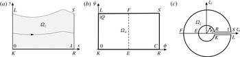
(a) One period of a
 $\unicode[STIX]{x1D706}$
-periodic domain in the physical
 $z$
-plane, (b) plane of the complex potential
 $w=\unicode[STIX]{x1D719}+\text{i}\unicode[STIX]{x1D713}$
, (c) parametric
 $\unicode[STIX]{x1D701}$
-plane.

2 Geometric interpretation of the Luke variational principle for steady periodic gravity waves
Consider a steady two-dimensional irrotational flow of an ideal incompressible fluid in an infinite
 $\unicode[STIX]{x1D706}$
-periodic domain bounded by a
 $\unicode[STIX]{x1D706}$
-periodic line
 $y=\unicode[STIX]{x1D702}(x)$
from above and by a horizontal bottom
 $y=0$
from below. One period
 $\unicode[STIX]{x1D6FA}_{z}$
of such a flow is shown in figure 1(a). The function
 $\unicode[STIX]{x1D702}(x)$
satisfies the conditions
 $$\begin{eqnarray}\displaystyle \unicode[STIX]{x1D702}(x)>0,\quad \unicode[STIX]{x1D702}(x+\unicode[STIX]{x1D706})=\unicode[STIX]{x1D702}(x). & & \displaystyle\end{eqnarray}$$
Let
 $\unicode[STIX]{x1D719}(x,y)$
be the potential of the flow. For the harmonic function
 $\unicode[STIX]{x1D719}(x,y)$
, we have the following boundary conditions
 $$\begin{eqnarray}\displaystyle \left[\frac{\unicode[STIX]{x2202}\unicode[STIX]{x1D719}}{\unicode[STIX]{x2202}n}\right]_{y=\unicode[STIX]{x1D702}(x)}=0,\quad \left[\frac{\unicode[STIX]{x2202}\unicode[STIX]{x1D719}}{\unicode[STIX]{x2202}n}\right]_{y=0}=-\left[\frac{\unicode[STIX]{x2202}\unicode[STIX]{x1D719}}{\unicode[STIX]{x2202}y}\right]_{y=0}=0, & & \displaystyle\end{eqnarray}$$
where
 $\boldsymbol{n}$
is the unit outer normal to the boundaries of the flow domain. The velocity vector
 $\boldsymbol{q}$
and its components
 $u$
,
 $v$
are
 $$\begin{eqnarray}\displaystyle \boldsymbol{q}=\unicode[STIX]{x1D735}\unicode[STIX]{x1D719},\quad u=\frac{\unicode[STIX]{x2202}\unicode[STIX]{x1D719}}{\unicode[STIX]{x2202}x},\quad v=\frac{\unicode[STIX]{x2202}\unicode[STIX]{x1D719}}{\unicode[STIX]{x2202}y}, & & \displaystyle\end{eqnarray}$$
where
 $\unicode[STIX]{x1D735}$
is the nabla operator. The volume flux
 $Q$
is
 $$\begin{eqnarray}\displaystyle Q=\int _{0}^{\unicode[STIX]{x1D702}(x)}u(x,y)\,\text{d}y. & & \displaystyle\end{eqnarray}$$
We assume that
 $Q>0$
, i.e. the fluid moves from left to right.
In the flow domain, the components of the velocity vector
 $u(x,y)$
,
 $v(x,y)$
are
 $\unicode[STIX]{x1D706}$
-periodic functions with respect to the variable
 $x$
, but the potential
 $\unicode[STIX]{x1D719}(x,y)$
increases by an increment
 $C$
(by a circulation) on every period:
 $$\begin{eqnarray}\displaystyle \unicode[STIX]{x1D719}(x+\unicode[STIX]{x1D706},y)-\unicode[STIX]{x1D719}(x,y)=C. & & \displaystyle\end{eqnarray}$$
For a fixed upper boundary the flow is defined uniquely by specifying the circulation
 $C$
.
Consider now a system of two-dimensional irrotational periodic waves of wavelength
 $\unicode[STIX]{x1D706}$
propagating with phase velocity
 $c$
under the influence of gravity
 $g$
without change of form from right to left on the surface of a fluid of finite depth. In the wave-fixed frame of reference the flow appears to be steady. Hence, we have a
 $\unicode[STIX]{x1D706}$
-periodic flow which moves from left to right, and its potential
 $\unicode[STIX]{x1D719}(x,y)$
satisfies the boundary conditions (2.2).
In addition to (2.2), on the unknown free surface
 $y=\unicode[STIX]{x1D702}(x)$
the Bernoulli equation should be fulfilled:
 $$\begin{eqnarray}\displaystyle \left[{\textstyle \frac{1}{2}}q^{2}+gy\right]_{y=\unicode[STIX]{x1D702}(x)}=R, & & \displaystyle\end{eqnarray}$$
where
 $q=|\unicode[STIX]{x1D735}\unicode[STIX]{x1D719}|$
is the modulus of the velocity vector
 $\boldsymbol{q}$
and
 $R$
is the Bernoulli constant. Thus, the steady gravity wave problem is fully determined by the boundary conditions (2.2), (2.6) at specified values of
 $\unicode[STIX]{x1D706}$
,
 $C$
and
 $R$
.
For the
 $\unicode[STIX]{x1D706}$
-periodic flows, consider the Luke Lagrangian, which we take as the integral of pressure over one period (see Luke Reference Luke1967):
 $$\begin{eqnarray}\displaystyle L=\frac{1}{\unicode[STIX]{x1D70C}}\int _{0}^{\unicode[STIX]{x1D706}}\,\text{d}x\int _{0}^{\unicode[STIX]{x1D702}(x)}p(x,y)\,\text{d}y, & & \displaystyle\end{eqnarray}$$
where
 $\unicode[STIX]{x1D70C}$
is the density of the fluid,
 $p$
is the pressure. At fixed
 $R$
and
 $C$
by virtue of the Bernoulli equation,
 $$\begin{eqnarray}\displaystyle \frac{p}{\unicode[STIX]{x1D70C}}=R-\frac{q^{2}}{2}-gy, & & \displaystyle\end{eqnarray}$$
so the functional
 $L$
depends only on
 $\unicode[STIX]{x1D702}(x)$
because
 $q(x,y)=|\unicode[STIX]{x1D735}\unicode[STIX]{x1D719}|$
is fully determined by the boundary condition (2.2). Hence, we can write
 $$\begin{eqnarray}\displaystyle L[\unicode[STIX]{x1D702}]=\int _{0}^{\unicode[STIX]{x1D706}}\,\text{d}x\int _{0}^{\unicode[STIX]{x1D702}(x)}\left(R-\frac{1}{2}|\unicode[STIX]{x1D735}\unicode[STIX]{x1D719}|^{2}-gy\right)\,\text{d}y.\hspace{-10.00002pt} & & \displaystyle\end{eqnarray}$$
Varying the functional
 $L[\unicode[STIX]{x1D702}]$
at a fixed
 $R$
, we obtain
 $$\begin{eqnarray}\displaystyle \unicode[STIX]{x1D6FF}L[\unicode[STIX]{x1D702}]=\int _{0}^{\unicode[STIX]{x1D706}}\left(R-\frac{1}{2}q^{2}[x,\unicode[STIX]{x1D702}(x)]-g\unicode[STIX]{x1D702}(x)\right)\unicode[STIX]{x1D6FF}\unicode[STIX]{x1D702}(x)\,\text{d}x-\iint _{\unicode[STIX]{x1D6FA}_{z}}\unicode[STIX]{x1D735}(\unicode[STIX]{x1D6FF}\unicode[STIX]{x1D719})\boldsymbol{\cdot }\unicode[STIX]{x1D735}\unicode[STIX]{x1D719}\,\text{d}x\,\text{d}y, & & \displaystyle\end{eqnarray}$$
where
 $\unicode[STIX]{x1D6FF}\unicode[STIX]{x1D719}(x,y)$
is the dependent variation of the potential
 $\unicode[STIX]{x1D719}(x,y)$
corresponding to the independent variation
 $\unicode[STIX]{x1D6FF}\unicode[STIX]{x1D702}(x)$
.
Applying Green’s first identity to the second integral in (2.10) and taking into account that the function
 $\unicode[STIX]{x1D719}(x,y)$
is harmonic, we get
 $$\begin{eqnarray}\displaystyle \iint _{\unicode[STIX]{x1D6FA}_{z}}\unicode[STIX]{x1D735}(\unicode[STIX]{x1D6FF}\unicode[STIX]{x1D719})\boldsymbol{\cdot }\unicode[STIX]{x1D735}\unicode[STIX]{x1D719}\,\text{d}x\,\text{d}y=\oint _{\unicode[STIX]{x2202}\unicode[STIX]{x1D6FA}_{z}}\unicode[STIX]{x1D6FF}\unicode[STIX]{x1D719}\frac{\unicode[STIX]{x2202}\unicode[STIX]{x1D719}}{\unicode[STIX]{x2202}n}\,\text{d}s, & & \displaystyle\end{eqnarray}$$
where
 $\unicode[STIX]{x2202}\unicode[STIX]{x1D6FA}_{z}$
is the boundary of
 $\unicode[STIX]{x1D6FA}_{z}$
,
 $\boldsymbol{n}$
is the unit outer normal to
 $\unicode[STIX]{x2202}\unicode[STIX]{x1D6FA}_{z}$
,
 $\text{d}s$
is the line element along
 $\unicode[STIX]{x2202}\unicode[STIX]{x1D6FA}_{z}$
. By virtue of (2.2), the contour integrals over
 $y=\unicode[STIX]{x1D702}(x)$
and
 $y=0$
vanish. Further, the integrals along the vertical lines
 $x=0$
and
 $x=\unicode[STIX]{x1D706}$
cancel each other. Indeed, because the circulation
 $C$
is fixed,
 $$\begin{eqnarray}\displaystyle \unicode[STIX]{x1D6FF}\unicode[STIX]{x1D719}(\unicode[STIX]{x1D706},y)-\unicode[STIX]{x1D6FF}\unicode[STIX]{x1D719}(0,y)=\unicode[STIX]{x1D6FF}C=0. & & \displaystyle\end{eqnarray}$$
Besides, the function
 $u(x,y)$
is
 $\unicode[STIX]{x1D706}$
-periodic with respect to
 $x$
, and on the vertical lines, we have
 $$\begin{eqnarray}\displaystyle \left[\frac{\unicode[STIX]{x2202}\unicode[STIX]{x1D719}}{\unicode[STIX]{x2202}n}\right]_{x=0}=-u(0,y),\quad \left[\frac{\unicode[STIX]{x2202}\unicode[STIX]{x1D719}}{\unicode[STIX]{x2202}n}\right]_{x=\unicode[STIX]{x1D706}}=u(\unicode[STIX]{x1D706},y)=u(0,y). & & \displaystyle\end{eqnarray}$$
Thus, the variation
 $$\begin{eqnarray}\displaystyle \unicode[STIX]{x1D6FF}L[\unicode[STIX]{x1D702}]=\int _{0}^{\unicode[STIX]{x1D706}}\left\{R-\frac{1}{2}q^{2}[x,\unicode[STIX]{x1D702}(x)]-g\unicode[STIX]{x1D702}(x)\right\}\unicode[STIX]{x1D6FF}\unicode[STIX]{x1D702}(x)\,\text{d}x & & \displaystyle\end{eqnarray}$$
under the constrain that
 $C$
is fixed. It follows from (2.14) that for
 $\unicode[STIX]{x1D706}$
-periodic flows with a fixed circulation
 $C$
, the dynamic boundary condition (2.6) will be satisfied if and only if
 $\unicode[STIX]{x1D6FF}L[\unicode[STIX]{x1D702}]$
=0.
It is to be noted that for any
 $\unicode[STIX]{x1D706}$
-periodic flow
 $$\begin{eqnarray}\displaystyle \iint _{\unicode[STIX]{x1D6FA}_{z}}q^{2}(x,y)\,\text{d}x\,\text{d}y=CQ & & \displaystyle\end{eqnarray}$$
(see, e.g. paper 1, p. 297).
Let
 $z=x+\text{i}y$
be the complex variable. In the plane
 $w=\unicode[STIX]{x1D719}+\text{i}\unicode[STIX]{x1D713}$
, consider the rectangle
 $\unicode[STIX]{x1D6FA}_{w}$
of length
 $C$
and width
 $Q$
, which corresponds to the flow period
 $\unicode[STIX]{x1D6FA}_{z}$
in the physical
 $z$
-plane (see figure 1
a,b). By means of the function
 $$\begin{eqnarray}\displaystyle \unicode[STIX]{x1D701}=r_{0}\exp \left(-\frac{2\unicode[STIX]{x03C0}w\text{i}}{C}\right),\quad \text{where }r_{0}=\exp \left(-\frac{2\unicode[STIX]{x03C0}Q}{C}\right), & & \displaystyle\end{eqnarray}$$
we map conformally
 $\unicode[STIX]{x1D6FA}_{w}$
onto an annulus with an outer radius of unity and inner radius of
 $r_{0}$
(see figure 1
b,c). It follows from (2.16) that
 $$\begin{eqnarray}\displaystyle Q=-\frac{C}{2\unicode[STIX]{x03C0}}\log r_{0}. & & \displaystyle\end{eqnarray}$$
Taking into account (2.9), (2.15) and (2.17), we come to the formula
 $$\begin{eqnarray}\displaystyle L[\unicode[STIX]{x1D702}]=\int _{0}^{\unicode[STIX]{x1D706}}\,\text{d}x\int _{0}^{\unicode[STIX]{x1D702}(x)}(R-gy)\,\text{d}y+\frac{c_{a}^{2}\unicode[STIX]{x1D706}^{2}}{4\unicode[STIX]{x03C0}}\log r_{0}, & & \displaystyle\end{eqnarray}$$
where
 $$\begin{eqnarray}\displaystyle c_{a}=\frac{C}{\unicode[STIX]{x1D706}}=\frac{1}{\unicode[STIX]{x1D706}}\int _{0}^{\unicode[STIX]{x1D706}}u(x,y)\,\text{d}x & & \displaystyle\end{eqnarray}$$
is the averaged horizontal component of velocity at any level
 $y=\text{const.}$
completely within the fluid.
As in Longuet-Higgins (Reference Longuet-Higgins1975) and many other works, we non-dimensionalize all flow parameters by choosing
 $\unicode[STIX]{x1D706}/(2\unicode[STIX]{x03C0})$
,
 $\sqrt{g\unicode[STIX]{x1D706}/(2\unicode[STIX]{x03C0})}$
and
 $\unicode[STIX]{x1D70C}$
as the scales for length, velocity and density, respectively. In what follows, all physical quantities will be dimensionless with accordance to the chosen scales. Now, the dimensionless wavelength is
 $2\unicode[STIX]{x03C0}$
,
 $\unicode[STIX]{x1D70C}=g=1$
, the potential
 $\unicode[STIX]{x1D719}$
, circulation
 $C$
and flux
 $Q$
are scaled by
 $\sqrt{g\unicode[STIX]{x1D706}^{3}/(2\unicode[STIX]{x03C0})^{3}}$
. The relation between
 $Q$
and
 $c_{a}$
is
 $$\begin{eqnarray}\displaystyle Q=-c_{a}\log r_{0}. & & \displaystyle\end{eqnarray}$$
The Luke functional
 $L$
, scaled by
 $g\unicode[STIX]{x1D706}^{2}/(2\unicode[STIX]{x03C0})^{2}$
, takes the form (for convenience, we double the functional and divide it by
 $\unicode[STIX]{x1D706}$
)
 $$\begin{eqnarray}\displaystyle L[\unicode[STIX]{x1D702}]=2Rh_{a}-H_{a}^{2}+c_{a}^{2}\log r_{0}, & & \displaystyle\end{eqnarray}$$
where
 $h_{a}$
and
 $H_{a}$
are the mean and root-mean-square depths:
 $$\begin{eqnarray}\displaystyle h_{a}=\frac{1}{2\unicode[STIX]{x03C0}}\int _{0}^{2\unicode[STIX]{x1D70B}}\unicode[STIX]{x1D702}(x)\,\text{d}x,\quad H_{a}^{2}=\frac{1}{2\unicode[STIX]{x03C0}}\int _{0}^{2\unicode[STIX]{x1D70B}}\unicode[STIX]{x1D702}^{2}(x)\,\text{d}x. & & \displaystyle\end{eqnarray}$$
Any
 $2\unicode[STIX]{x03C0}$
-periodic domain can be transformed into a doubly connected one by means of the conformal mapping
 $t=\exp (\text{i}z)$
. The conformal invariant
 $M$
, that is defined as the ratio
 $r_{1}/r_{2}$
(
 $r_{1}>r_{2}$
) of the radii of an annulus onto which the doubly connected domain can be mapped, is called the modulus of the domain (see Bergman Reference Bergman1950, p. 102). Taking into account that in our case
 $M=1/r_{0}$
, one can see that the Luke Lagrangian
 $L$
in the form (2.21) contains only geometric characteristics of
 $2\unicode[STIX]{x03C0}$
-periodic domains: the mean depths and the modulus. In terms of these geometric characteristics, the variational principal can be formulated in the form of the following proposition.
Proposition 1. A
 $2\unicode[STIX]{x03C0}$
-periodic domain is that of steady gravity waves if and only if
 $$\begin{eqnarray}\displaystyle \unicode[STIX]{x1D6FF}L[\unicode[STIX]{x1D702}]=\unicode[STIX]{x1D6FF}(2R\;h_{a}-H_{a}^{2}+c_{a}^{2}\log r_{0})=0, & & \displaystyle\end{eqnarray}$$
where the parameters
 $R$
and
 $c_{a}^{2}$
are fixed.
The parameter
 $r_{0}$
is responsible for the wave depth-to-length ratio and ranges between 0 and 1. For the waves of infinite depth
 $r_{0}$
=0, for the solitary waves
 $r_{0}=1$
. Application of the functional (2.21) is especially convenient when the parameter
 $r_{0}$
is given, as for example, in computations by Schwartz (Reference Schwartz1974) and Cokelet (Reference Cokelet1977). Indeed, in this case, at fixed
 $c_{a}$
the variation
 $\unicode[STIX]{x1D6FF}(c_{a}\log r_{0})=0$
, and the functional
 $L[\unicode[STIX]{x1D702}]$
is equivalent to
 $$\begin{eqnarray}\displaystyle L_{M}[\unicode[STIX]{x1D702}]=2R\;h_{a}-H_{a}^{2}. & & \displaystyle\end{eqnarray}$$
So we can formulate the following proposition.
Proposition 2. In the class of
 $2\unicode[STIX]{x03C0}$
-periodic domains with the same modulus
 $M=1/r_{0}$
, the domain of periodic gravity waves is that for which
 $$\begin{eqnarray}\displaystyle \unicode[STIX]{x1D6FF}L_{M}[\unicode[STIX]{x1D702}]=0, & & \displaystyle\end{eqnarray}$$
where in (2.24) the parameter
 $R$
is fixed.
We consider Propositions 1 and 2 as a geometric interpretation of the Luke variational principle.
3 System of quadratic equations for the Stokes coefficients
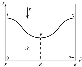
Let us assume that the waves are symmetric and the axis of ordinate is that of symmetry which goes through one of the wave crests. One period of the flow is shown in figure 2. We shall seek the conformal mapping of the annulus (figure 1
c) in the parametric
 $\unicode[STIX]{x1D701}$
-plane onto the flow domain of one wave period
 $\unicode[STIX]{x1D6FA}_{z}$
in the form
 $$\begin{eqnarray}\displaystyle z(\unicode[STIX]{x1D701})=2\unicode[STIX]{x03C0}+\text{i}\log \unicode[STIX]{x1D701}-\text{i}\log r_{0}+\text{i}\mathop{\sum }_{n=1}^{\infty }y_{n}\left(\unicode[STIX]{x1D701}^{n}-\frac{r_{0}^{2n}}{\unicode[STIX]{x1D701}^{n}}\right). & & \displaystyle\end{eqnarray}$$
The representation (3.1) is a variant of the second Stokes method, suggested by Schwartz (Reference Schwartz1974). By virtue of the wave symmetry, the Stokes coefficients
 $y_{n}$
(
 $n=1,2,3\ldots$
) are real. Moreover, for the representation (3.1) the condition on the bottom
 $\text{Im}z=0$
is automatically fulfilled. The parametric equations of the free surface are
 $$\begin{eqnarray}\displaystyle \hspace{-12.0pt}x_{s}(\unicode[STIX]{x1D6FE})=2\unicode[STIX]{x03C0}-\unicode[STIX]{x1D6FE}-\mathop{\sum }_{n=1}^{\infty }\unicode[STIX]{x1D6FC}_{n}y_{n}\sin n\unicode[STIX]{x1D6FE},\quad y_{s}(\unicode[STIX]{x1D6FE})=-\log r_{0}+\mathop{\sum }_{n=1}^{\infty }\unicode[STIX]{x1D6FD}_{n}y_{n}\cos n\unicode[STIX]{x1D6FE},\hspace{12.0pt} & & \displaystyle\end{eqnarray}$$
where
 $\unicode[STIX]{x1D6FC}_{n}=1+r_{0}^{2n}$
,
 $\unicode[STIX]{x1D6FD}_{n}=1-r_{0}^{2n}$
,
 $\unicode[STIX]{x1D6FE}$
is the polar angle in the
 $\unicode[STIX]{x1D701}$
-plane.
One wave period in the physical
 $z$
-plane.

It is to be noted that the mapping (3.1) specifies a family of
 $2\unicode[STIX]{x03C0}$
-periodic domains with the same modulus
 $M=1/r_{0}$
. Thus, we are under the conditions of Proposition 2. In appendix A to the paper, it will be proved that
 $$\begin{eqnarray}\displaystyle h_{a}={\textstyle \frac{1}{2}}\unicode[STIX]{x1D6EC}-\log r_{0},\quad H_{a}^{2}={\textstyle \frac{1}{2}}(\unicode[STIX]{x1D6EC}_{1}+G)-\unicode[STIX]{x1D6EC}\log r_{0}+\log ^{2}r_{0}, & & \displaystyle\end{eqnarray}$$
where
 $$\begin{eqnarray}\displaystyle \unicode[STIX]{x1D6EC}=\mathop{\sum }_{n=1}^{\infty }n\unicode[STIX]{x1D6FD}_{2n}y_{n}^{2},\quad \unicode[STIX]{x1D6EC}_{1}=\mathop{\sum }_{n=1}^{\infty }\unicode[STIX]{x1D6FD}_{n}^{2}y_{n}^{2},\quad G=\mathop{\sum }_{k=2}^{\infty }y_{k}\mathop{\sum }_{n=1}^{k-1}\unicode[STIX]{x1D6E4}_{k-n,n}y_{n}y_{k-n}, & & \displaystyle\end{eqnarray}$$
 $$\begin{eqnarray}\displaystyle \unicode[STIX]{x1D6FD}_{n}=1-r_{0}^{2n},\quad \unicode[STIX]{x1D6E4}_{m,n}=m\unicode[STIX]{x1D6FD}_{n}\unicode[STIX]{x1D6FD}_{2m+n}+n\unicode[STIX]{x1D6FD}_{m}\unicode[STIX]{x1D6FD}_{m+2n}. & & \displaystyle\end{eqnarray}$$
Inserting (3.3) into (2.24) yields
 $$\begin{eqnarray}\displaystyle L_{M}=(R+\log r_{0})\unicode[STIX]{x1D6EC}-{\textstyle \frac{1}{2}}(\unicode[STIX]{x1D6EC}_{1}+G)-\log ^{2}r_{0}-2R\log r_{0}. & & \displaystyle\end{eqnarray}$$
It follows from (3.4) and (3.5) that
 $L_{M}$
is a function of the Stokes coefficients
 $y_{n}$
(
 $n=1,2,3,\ldots$
) and the parameter
 $r_{0}$
. In accordance with (2.25) of Proposition 2, we variate
 $L_{M}$
with respect to
 $y_{n}$
at fixed
 $r_{0}$
to get
 $$\begin{eqnarray}\displaystyle (n\unicode[STIX]{x1D6FD}_{2n}K-\unicode[STIX]{x1D6FD}_{n}^{2})y_{n}=\frac{1}{2}\frac{\unicode[STIX]{x2202}G}{\unicode[STIX]{x2202}y_{n}},\quad n=1,2,3,\ldots , & & \displaystyle\end{eqnarray}$$
where
 $$\begin{eqnarray}\displaystyle K=2(R+\log r_{0}). & & \displaystyle\end{eqnarray}$$
In appendix A to the paper, we shall prove that
 $$\begin{eqnarray}\displaystyle \frac{\unicode[STIX]{x2202}G}{\unicode[STIX]{x2202}y_{n}}=\mathop{\sum }_{m=1}^{n-1}\unicode[STIX]{x1D6E4}_{n-m,m}y_{n-m}y_{m}+2\mathop{\sum }_{m=1}^{\infty }\unicode[STIX]{x1D6E4}_{m,n}y_{m+n}y_{m}. & & \displaystyle\end{eqnarray}$$
With allowance for (3.9) we deduce
 $$\begin{eqnarray}\displaystyle \hspace{-12.0pt}(n\unicode[STIX]{x1D6FD}_{2n}K-\unicode[STIX]{x1D6FD}_{n}^{2})y_{n}=\frac{1}{2}\mathop{\sum }_{m=1}^{n-1}\unicode[STIX]{x1D6E4}_{n-m,m}y_{n-m}y_{m}+\mathop{\sum }_{m=1}^{\infty }\unicode[STIX]{x1D6E4}_{m,n}y_{m+n}y_{m},\quad n=1,2,3,\ldots \hspace{12.0pt} & & \displaystyle\end{eqnarray}$$
and at
 $n=1$
the first sum in (3.10) vanishing. The system (3.10) is an infinite system of quadratic equations with respect to the Stokes coefficients
 $y_{n}$
.
Equation (2.23) of Proposition 1 allows us to express
 $c_{a}^{2}$
in terms of the Stokes coefficients. Indeed, fixing
 $y_{n}$
and varying only
 $r_{0}$
, we obtain
 $$\begin{eqnarray}\displaystyle c_{a}^{2}=-r_{0}\frac{\unicode[STIX]{x2202}L_{M}}{\unicode[STIX]{x2202}r_{0}}=K-\unicode[STIX]{x1D6EC}+\frac{r_{0}}{2}\left(\frac{\unicode[STIX]{x2202}\unicode[STIX]{x1D6EC}_{1}}{\unicode[STIX]{x2202}r_{0}}+\frac{\unicode[STIX]{x2202}G}{\unicode[STIX]{x2202}r_{0}}-K\frac{\unicode[STIX]{x2202}\unicode[STIX]{x1D6EC}}{\unicode[STIX]{x2202}r_{0}}\right), & & \displaystyle\end{eqnarray}$$
where
 $$\begin{eqnarray}\displaystyle \frac{\unicode[STIX]{x2202}\unicode[STIX]{x1D6EC}}{\unicode[STIX]{x2202}r_{0}}=\mathop{\sum }_{n=1}^{\infty }n\frac{\text{d}\unicode[STIX]{x1D6FD}_{2n}}{\text{d}r_{0}}y_{n}^{2},\quad \frac{\unicode[STIX]{x2202}\unicode[STIX]{x1D6EC}_{1}}{\unicode[STIX]{x2202}r_{0}}=\mathop{\sum }_{n=1}^{\infty }2\unicode[STIX]{x1D6FD}_{n}\frac{\text{d}\unicode[STIX]{x1D6FD}_{n}}{\text{d}r_{0}}y_{n}^{2}, & & \displaystyle\end{eqnarray}$$
 $$\begin{eqnarray}\displaystyle \frac{\unicode[STIX]{x2202}G}{\unicode[STIX]{x2202}r_{0}}=\mathop{\sum }_{k=2}^{\infty }y_{k}\mathop{\sum }_{n=1}^{k-1}\frac{\text{d}\unicode[STIX]{x1D6E4}_{k-n,n}}{\text{d}r_{0}}y_{n}y_{k-n}. & & \displaystyle\end{eqnarray}$$
The conformal mapping of the annulus
 $\unicode[STIX]{x1D6FA}_{\unicode[STIX]{x1D701}}$
onto the rectangle
 $\unicode[STIX]{x1D6FA}_{w}$
in the
 $w$
-plane (see figure 1
b,c) is determined by the equation
 $$\begin{eqnarray}\displaystyle w=c_{a}\text{i}(\log \unicode[STIX]{x1D701}-\log r_{0}-2\unicode[STIX]{x03C0}\text{i}). & & \displaystyle\end{eqnarray}$$
If the depth of the fluid is infinite, then
 $r_{0}\rightarrow 0$
,
 $\unicode[STIX]{x1D6FD}_{n}=1$
,
 $\unicode[STIX]{x1D6E4}_{m,n}=m+n$
, and the system (3.10) becomes simpler:
 $$\begin{eqnarray}\displaystyle (nK-1)y_{n}=\frac{n}{2}\mathop{\sum }_{m=1}^{n-1}y_{n-m}y_{m}+\mathop{\sum }_{m=1}^{\infty }(m+n)y_{m+n}y_{m},\quad n=1,2,3,\ldots & & \displaystyle\end{eqnarray}$$
Equation (3.11) transforms to the relation
 $$\begin{eqnarray}\displaystyle c_{a}^{2}=K-\unicode[STIX]{x1D6EC}. & & \displaystyle\end{eqnarray}$$
If
 $r_{0}\rightarrow 0$
, then
 $\log r_{0}\rightarrow -\infty$
, and the formula of the conformal mapping (3.1) loses its sense. To avoid this, it is enough to transfer the
 $x$
-axes of the
 $z$
-plane onto the mean level of waves by setting
 $z_{1}=z-\text{i}h_{a}$
. It follows from (3.3a
) that
 $\log r_{0}=\unicode[STIX]{x1D6EC}/2-h_{a}$
, and then for the infinite depth,
 $$\begin{eqnarray}\displaystyle z_{1}(\unicode[STIX]{x1D701})=2\unicode[STIX]{x03C0}+\text{i}\log \unicode[STIX]{x1D701}-\text{i}\frac{\unicode[STIX]{x1D6EC}}{2}+\text{i}\mathop{\sum }_{n=1}^{\infty }y_{n}\unicode[STIX]{x1D701}^{n}. & & \displaystyle\end{eqnarray}$$
Thus, for the fixed parameters
 $K=2(R+\log r_{0})$
and
 $r_{0}$
, any non-trivial solution to system (3.10) and formulae (3.1), (3.14) define a
 $2\unicode[STIX]{x03C0}$
-periodic wave domain and the parametric equations for the complex potential
 $w$
.
We should remark that Schwartz (Reference Schwartz1974), and later Cokelet (Reference Cokelet1977), located the
 $x$
-axes in the physical plane at the level
 $d$
above the bottom, defining
 $d$
as the depth of uniform stream flowing with speed
 $c_{a}$
whose mass flux equals that of the wave. Hence,
 $d=Q/c_{a}$
. Since
 $Q=-c_{a}\log r_{0}$
, it is clear that
 $d=-\log r_{0}$
. This elucidates the physical sense of the parameter
 $K$
in system (3.10). Indeed, by virtue of (2.6) and (3.8), on the free surface we have
 $$\begin{eqnarray}\displaystyle [q^{2}+2(y-d)]_{y=\unicode[STIX]{x1D702}(x)}=K. & & \displaystyle\end{eqnarray}$$
This means that the parameter
 $K$
is simply the Bernoulli constant as it was defined and designated in Schwartz (Reference Schwartz1974) and Cokelet (Reference Cokelet1977). If in solving system (3.10) we specify another parameter instead of
 $K$
, for example,
 $y_{1}$
as in Stokes (Reference Stokes1880), then (3.10) is a pure quadratic system of equations with respect to the unknowns
 $K$
and
 $y_{n}$
.
4 Algorithm for solving system (3.10)
Let
 $a$
be the amplitude of the wave (one half the vertical distance from the crest to the trough). The goal of this section is to develop an algorithm for finding expansions for the Stokes coefficient
 $y_{n}$
in powers of the wave amplitude
 $a$
with coefficients depending on the mean depth
 $h_{a}$
.
Because in system (3.10) the coefficients
 $\unicode[STIX]{x1D6FD}_{n}$
and
 $\unicode[STIX]{x1D6E4}_{m,n}$
depend only on
 $r_{0}^{2}$
, it is convenient to introduce
 $$\begin{eqnarray}\displaystyle r=r_{0}^{2},\quad \text{and hence,}\quad \unicode[STIX]{x1D6FD}_{n}=1-r^{n}. & & \displaystyle\end{eqnarray}$$
Now in (3.10), the coefficients
 $\unicode[STIX]{x1D6FD}_{n}$
,
 $\unicode[STIX]{x1D6E4}_{m,n}$
depend on
 $r$
, formula (3.11) for
 $c_{a}^{2}$
transforms to
 $$\begin{eqnarray}\displaystyle c_{a}^{2}=K-\unicode[STIX]{x1D6EC}+r\left(\frac{\unicode[STIX]{x2202}\unicode[STIX]{x1D6EC}_{1}}{\unicode[STIX]{x2202}r}\right.+\left.\frac{\unicode[STIX]{x2202}G}{\unicode[STIX]{x2202}r}-K\frac{\unicode[STIX]{x2202}\unicode[STIX]{x1D6EC}}{\unicode[STIX]{x2202}r}\right), & & \displaystyle\end{eqnarray}$$
and in (3.12), (3.13) we need to replace
 $r_{0}$
by
 $r$
.
At the first step, we follow Stokes (Reference Stokes1880), namely, we assume that
 $y_{1}=b$
, where
 $b$
is a specified small parameter. Since
 $y_{1}$
is given, the parameter
 $K$
is now unknown. We shall seek the coefficients
 $y_{n}$
(
 $n=2,3,\ldots$
) and the parameter
 $K$
in the form of expansions in powers of
 $b$
. Let an odd number
 $N$
be the greatest power in these expansions, then
 $$\begin{eqnarray}\displaystyle K=\mathop{\sum }_{n=0}^{(N-1)/2}K_{2n}b^{2n}+O(b^{N+1}),\quad y_{i}=\mathop{\sum }_{n=0}^{[(N-i)/2]}b_{i,2n}b^{i+2n}+o(b^{N}),\quad i=2,3,\ldots ,N, & & \displaystyle \nonumber\\ \displaystyle & & \displaystyle\end{eqnarray}$$
where
 $[\;\;]$
denotes the integer part of a real number, and the coefficients
 $K_{2n}$
and
 $b_{i,2n}$
are to be found. The general number of unknown coefficients is
 $(N+1)^{2}/4$
. The procedure of their consecutive search appears as follows.
(i) We substitute the expressions for
 $K$
and
 $y_{i}$
from (4.3) in the first
 $N$
equations of system (3.10) and expand each of the equations into the series in powers of
 $b$
up to the power
 $N$
inclusively. We obtain
 $N$
equations of the form
 $P_{i}(b)=0$
,
 $i=1,2,\ldots ,N$
, where
 $P_{i}(b)$
are
 $N$
-degree polynomials in
 $b$
. The coefficients of these polynomials depend on the unknowns
 $K_{2n}$
and
 $b_{i,2n}$
. Equating these coefficients to zero, we obtain a system of
 $(N+1)^{2}/4$
equations with respect to
 $(N+1)^{2}/4$
unknowns
 $K_{2n}$
and
 $b_{i,2n}$
. It is to be noted that if
 $N$
is chosen to be even, then the number of unknowns will be greater by one than the number of equations, and not all coefficients will be found.
(ii) We organize the external loop for
 $j=1,2,\ldots ,N$
, where
 $j$
is the power of the parameter
 $b$
labelling the coefficients at
 $b^{j}$
in the polynomials
 $P_{i}(b)$
. Let the function
 $\lceil x\rceil$
designate a so called ‘ceiling’, i.e. the least integer greater than or equal to
 $x$
. The unknown coefficients
 $K_{2n}$
and
 $b_{i,2n}$
are determined by portions with
 $\lceil j/2\rceil$
coefficients in each portion. In the external loop over
 $j$
, we organize the internal loop for
 $k=1,2,\ldots ,\lceil j/2\rceil$
. For each
 $k$
we find
 $$\begin{eqnarray}\displaystyle i_{k}=j-2\lceil j/2\rceil +2k. & & \displaystyle\end{eqnarray}$$
We equate the coefficient at
 $b^{j}$
in the polynomial
 $P_{i_{k}}(b)$
to zero and from the obtained equation we find either
 $$\begin{eqnarray}\displaystyle K_{j-1}\;(\text{if }j\text{ is odd and }k=1)\quad \text{or}\quad b_{i_{k},j-i_{k}}\;(\text{if }j\text{ is even or }k\not =1), & & \displaystyle\end{eqnarray}$$
and in so doing all equations for finding
 $K_{j-1}$
or
 $b_{i_{k},j-i_{k}}$
being linear.
Formulae (4.4), (4.5) define exactly the consecutive procedure of determining
 $K_{2n}$
,
 $b_{i,2n}$
, and for each pair
 $(j,k)$
, allow us to express a new unknown coefficient in terms of the coefficients which have been already found. Note, by the way, that as follows from (4.5a
), if
 $N$
is even, then
 $K_{2N}$
remains indefinite.
The above algorithm results in the expansions (4.3) with coefficients which are rational functions of
 $r=r_{0}^{2}$
. Inserting these expansions into (4.2) gives
 $$\begin{eqnarray}\displaystyle c_{a}^{2}=\mathop{\sum }_{n=1}^{(N-1)/2}c_{2n}b^{2n}+O(b^{N+1}), & & \displaystyle\end{eqnarray}$$
where the coefficients
 $c_{2n}$
are also rational functions of
 $r$
.
The second step is to express the parameter
 $b$
in terms of the amplitude
 $a$
and to reconstruct the expansions (4.3) and (4.6) in powers of
 $a$
. It follows from (3.2b
) that
 $$\begin{eqnarray}\displaystyle a-\mathop{\sum }_{n=1}^{(N+1)/2}\unicode[STIX]{x1D6FD}_{2n-1}y_{2n-1}=0. & & \displaystyle\end{eqnarray}$$
Taking into account that the coefficients
 $y_{2n-1}$
contain only odd powers of
 $b$
, we shall seek the parameter
 $b$
as
 $$\begin{eqnarray}\displaystyle b=\mathop{\sum }_{n=1}^{(N+1)/2}b_{2n-1}a^{2n-1}. & & \displaystyle\end{eqnarray}$$
Substituting (4.8) into (4.7) and expanding the left-hand side of (4.7) in powers of
 $a$
up to the power
 $N$
inclusively, we obtain an
 $N$
-degree polynomial in odd powers of
 $a$
with
 $(N+1)/2$
coefficients depending on the parameter
 $r$
and the unknowns
 $b_{2n-1}$
. Equating these coefficients to zero, we sequently find
 $b_{1},b_{3},\ldots ,b_{N}$
, which again turn out to be rational functions of
 $r$
. Now we reconstruct the expansions (4.3) and (4.6) in powers of
 $a$
by inserting in these expansions the expression (4.8) for
 $b$
. As a result we have
 $$\begin{eqnarray}\displaystyle K=\mathop{\sum }_{n=0}^{(N-1)/2}K_{2n}^{\prime }a^{2n}+O(a^{N+1}),\quad c_{a}^{2}=\mathop{\sum }_{n=1}^{(N-1)/2}c_{2n}^{\prime }a^{2n}+O(a^{N+1}), & & \displaystyle\end{eqnarray}$$
 $$\begin{eqnarray}\displaystyle y_{i}=\mathop{\sum }_{n=0}^{[(N-i)/2]}b_{i,2n}^{\prime }a^{i+2n}+o(a^{N}),\quad i=1,2,\ldots ,N, & & \displaystyle\end{eqnarray}$$
where the coefficients
 $K_{2n}^{\prime }$
,
 $c_{2n}^{\prime }$
and
 $b_{i,2n}^{\prime }$
are rational functions of
 $r=r_{0}^{2}$
.
The third and last step is to express the parameter
 $r=r_{0}^{2}$
in terms of the mean depth
 $h_{a}$
and to reconstruct the expansions (4.9) and (4.10) so that they would be in powers of
 $a$
with coefficients depending
 $h_{a}$
. Let
 $\unicode[STIX]{x1D700}=\exp (-2h_{a})$
. It follows from (3.3a
) and (3.4a
) that
 $$\begin{eqnarray}\displaystyle r-\unicode[STIX]{x1D700}\exp \left(\mathop{\sum }_{n=1}^{(N-1)/2}n\unicode[STIX]{x1D6FD}_{2n}y_{n}^{2}\right)=0. & & \displaystyle\end{eqnarray}$$
We shall seek the dependence between
 $r$
and
 $\unicode[STIX]{x1D700}$
in the form
 $$\begin{eqnarray}\displaystyle r=\unicode[STIX]{x1D700}\left(1+\mathop{\sum }_{n=1}^{(N-1)/2}\unicode[STIX]{x1D708}_{2n}a^{2n}\right), & & \displaystyle\end{eqnarray}$$
where
 $\unicode[STIX]{x1D708}_{2n}$
are unknown coefficients depending on
 $\unicode[STIX]{x1D700}=\exp (-2h_{a})$
.
Substituting (4.12) into (4.11) and expanding the left-hand side of (4.11) in powers of
 $a$
up to the power
 $N-1$
inclusively, we obtain an
 $(N-1)$
-degree polynomial in even powers of
 $a$
with
 $(N-1)/2$
non-zero coefficients depending on the parameter
 $\unicode[STIX]{x1D700}$
and the unknowns
 $\unicode[STIX]{x1D708}_{2n}$
. The coefficient at
 $a^{0}$
in this polynomial is zero. Equating the remainder coefficients to zero, we sequently find
 $\unicode[STIX]{x1D708}_{2},\unicode[STIX]{x1D708}_{4},\ldots ,\unicode[STIX]{x1D708}_{N-1}$
, which are now rational functions of
 $\unicode[STIX]{x1D700}$
. Reconstruction of the expansions (4.9) and (4.10) by means of (4.12) yields
 $$\begin{eqnarray}\displaystyle K=\mathop{\sum }_{n=0}^{(N-1)/2}\unicode[STIX]{x1D705}_{2n}a^{2n}+O(a^{N+1}),\quad c_{a}^{2}=\mathop{\sum }_{n=1}^{(N-1)/2}\unicode[STIX]{x1D70E}_{2n}a^{2n}+O(a^{N+1}), & & \displaystyle\end{eqnarray}$$
 $$\begin{eqnarray}\displaystyle y_{i}=\mathop{\sum }_{n=0}^{[(N-i)/2]}a_{i,2n}a^{i+2n}+o(a^{N}),\quad i=1,2,\ldots ,N, & & \displaystyle\end{eqnarray}$$
where the coefficients
 $\unicode[STIX]{x1D705}_{2n}$
,
 $\unicode[STIX]{x1D70E}_{2n}$
and
 $a_{i,2n}$
are known rational functions of
 $\unicode[STIX]{x1D700}=\exp (-2h_{a})$
.
This algorithm has been realized by means of Mathematica package which allows symbolic computations and exact arithmetics to be applied (see Wolfram Reference Wolfram2003). In so doing, the routines Series, Coefficient and Solve have been used systematically. It is worth noticing that steps 1 and 2 of the algorithm correspond to the formulations by Schwartz (Reference Schwartz1974) and Cokelet (Reference Cokelet1977), when the depth
 $d=-\log r_{0}$
is fixed. The third step correspond to the formulations by De (Reference De1955) and Fenton (Reference Fenton1985), when instead of the parameter
 $d=-\log r_{0}$
, whose physical meaning is not quite clear, the mean wave depth
 $h_{a}$
is specified.
We should remark that the first two steps can be programmed in such computer languages as Fortran or C++, but the most time-consuming third step requires necessarily the symbolic computations because in (4.11) we need to know the coefficients
 $y_{n}$
as functions of
 $r$
and
 $a$
. Realizing all three steps, we have carried out the computations at
 $N=21$
.
5 Expansions for the wave resistance and other wave properties in terms of the geometric wave parameters:
 $h_{a}$
and
$a$


Applying the algorithm of § 4, we obtain the expansions (4.13) and (4.14) in powers of
 $a$
with coefficients which are rational functions of the parameter
 $\unicode[STIX]{x1D700}=\exp (-2h_{a})$
. As we shall see in what follows, finding the expansion for the wave resistance requires the knowledge of the expansions for the mean potential energy
 $V$
and the root-mean-square velocity
 $c_{b}$
at the bottom in steady motion, which are defined as
 $$\begin{eqnarray}\displaystyle V=\frac{1}{4\unicode[STIX]{x03C0}}\int _{0}^{2\unicode[STIX]{x03C0}}[\unicode[STIX]{x1D702}(x)-h_{a}]^{2}\,\text{d}x,\quad c_{b}^{2}=\frac{1}{2\unicode[STIX]{x03C0}}\int _{0}^{2\unicode[STIX]{x03C0}}u^{2}(\unicode[STIX]{x1D709},0)\,\text{d}\unicode[STIX]{x1D709}. & & \displaystyle\end{eqnarray}$$
It can be easily seen from the definitions of
 $V$
and
 $H_{a}^{2}$
that
 $V=(H_{a}^{2}-h_{a}^{2})/2$
. This relation and equations (3.3) yield
 $$\begin{eqnarray}\displaystyle V=\frac{1}{4}\left(\unicode[STIX]{x1D6EC}_{1}+G-\frac{\unicode[STIX]{x1D6EC}^{2}}{2}\right). & & \displaystyle\end{eqnarray}$$
Using (3.4) and (4.14), we get the expansion for
 $V$
. In so doing, the coefficients
 $\unicode[STIX]{x1D6FD}_{n}$
and
 $\unicode[STIX]{x1D6E4}_{mn}$
, which depend on
 $r$
, should be also expanded in powers of
 $a$
by means of formula (4.12).
For the parameter
 $c_{b}^{2}$
, it is possible to prove the identity
 $$\begin{eqnarray}\displaystyle c_{b}^{2}+2h_{a}=2R & & \displaystyle\end{eqnarray}$$
(see equation (3.22) in paper 1). From this identity and equations (3.3a ), (3.8) we conclude that
 $$\begin{eqnarray}\displaystyle c_{b}^{2}=K-\unicode[STIX]{x1D6EC}, & & \displaystyle\end{eqnarray}$$
which allows us to find the expansion for
 $c_{b}^{2}$
.
Implementation of the algorithm of § 4 and the above manipulations leads to expansions for the wave parameters
 $c_{a}^{2}$
,
 $c_{b}^{2}$
,
 $V$
,
 $\unicode[STIX]{x1D6EC}$
, which are needed to get the expansion for the wave resistance. All these expansions are in powers of
 $a$
with coefficients which are rational functions of
 $\unicode[STIX]{x1D700}=\exp (-2h_{a})$
. Besides, the expansions for
 $c_{a}^{2}$
,
 $c_{b}^{2}$
,
 $V$
and
 $\unicode[STIX]{x1D6EC}$
contain only even powers of
 $a$
, moreover, they possess a very useful feature: the numerators of their coefficients (but not denominators) are so-called palindromic polynomials of
 $\unicode[STIX]{x1D700}$
. By definition, a polynomial
 $P_{n}(\unicode[STIX]{x1D700})$
of degree
 $n$
is palindromic if
 $$\begin{eqnarray}\displaystyle P_{n}(\unicode[STIX]{x1D700})=\unicode[STIX]{x1D700}^{n}P_{n}(1/\unicode[STIX]{x1D700}). & & \displaystyle\end{eqnarray}$$
This feature allows us to shorten representations of polynomials by one-half, for example,
 $$\begin{eqnarray}\displaystyle P_{2}(2,3)=2+3\unicode[STIX]{x1D700}+2\unicode[STIX]{x1D700}^{2},\quad P_{3}(2,3)=2+3\unicode[STIX]{x1D700}+3\unicode[STIX]{x1D700}^{2}+2\unicode[STIX]{x1D700}^{3},\quad P_{4}(1,0,4)=1+4\unicode[STIX]{x1D700}^{2}+\unicode[STIX]{x1D700}^{4},\hspace{-10.00002pt} & & \displaystyle \nonumber\\ \displaystyle & & \displaystyle\end{eqnarray}$$
and so on.
In appendix B to the paper, formulae (B 1)–(B 4) present the expansions for
 $c_{a}^{2}$
,
 $c_{b}^{2}$
,
 $\unicode[STIX]{x1D6EC}$
and
 $V$
up to
 $a^{6}\,(N=7)$
. In spite of the fact that we have carried out the computations at
 $N=21$
, expansions for
 $N\geqslant 9$
become too long to be printed. For example, the formula for
 $c_{a}^{2}$
at
 $N=21$
after conversion to LaTeX takes approximately 75 kilobytes, i.e. approximately 25 journal pages. For completeness, an expansion for the mean kinetic energy
 $T_{c_{a}}$
, computed under the assumption that the waves propagate with the speed
 $c_{a}$
in the bottom-fixed reference frame, is also presented by (B 5). The expansion for
 $T_{c_{a}}$
can be easily obtained from (3.3a
) and formula (5.21) from the paper by Cokelet (Reference Cokelet1977):
 $$\begin{eqnarray}\displaystyle T_{c_{a}}={\textstyle \frac{1}{2}}c_{a}^{2}(h_{a}+\log r_{0})={\textstyle \frac{1}{4}}c_{a}^{2}\unicode[STIX]{x1D6EC}. & & \displaystyle\end{eqnarray}$$
In paper 1, we have derived formula (3.13) for the wave resistance
 $R_{w}$
of a two-dimensional body that moves horizontally at a constant speed
 $c$
in a channel of finite depth
 $h$
. In dimensionless form, this formula can be written as
 $$\begin{eqnarray}\displaystyle R_{w}=3V+{\textstyle \frac{3}{2}}\unicode[STIX]{x1D6FF}_{1}^{2}+(h-c^{2})\unicode[STIX]{x1D6FF}_{1}, & & \displaystyle\end{eqnarray}$$
where
 $\unicode[STIX]{x1D6FF}_{1}=h_{a}-h$
is the defect of levels (the difference between the mean level far downstream and the undisturbed level far upstream). The scale for
 $R_{w}$
in (5.8) is
 $\unicode[STIX]{x1D70C}g\unicode[STIX]{x1D706}^{2}/(2\unicode[STIX]{x03C0})^{2}$
. The formula has been derived under assumptions that in the body-fixed reference frame the flow is steady and irrotational.
Assume that for the waves far downstream we know the mean depth
 $h_{a}$
and amplitude
 $a$
. The knowledge of these parameters is enough to compute all wave properties, but to find the wave resistance by means of (5.8), we should determine the parameters
 $c$
and
 $h$
. In a sense, this is an inverse problem: in the body-fixed reference frame find the speed
 $c$
and depth
 $h$
of a uniform stream which without dissipation is able to create a given system of waves far downstream due to some disturbance located in the stream.
By virtue of the fact that the Bernoulli constant
 $R$
and the flow flux
 $Q$
far upstream and far downstream are the same, the parameters
 $c$
and
 $h$
satisfy the following system of equations
 $$\begin{eqnarray}\displaystyle \frac{c^{2}}{2}+h=R,\quad ch=Q, & & \displaystyle\end{eqnarray}$$
where
 $R$
and
 $Q$
are known wave properties. With the help of some results obtained in the works by Keady & Norbury (Reference Keady and Norbury1975) and Benjamin (Reference Benjamin1995), it has been demonstrated in paper 1 that system (5.9) always has two solutions,
 $(c_{1},h_{1})$
and
 $(c_{2},h_{2})$
. For the first solution, the Froude number
 $Fr=c_{1}/\sqrt{h_{1}}<1$
, for the second one, the Froude number
 $Fr=c_{2}/\sqrt{h_{2}}>1$
. So, for the first solution, the upstream flow is subcritical, for the second one, it is supercritical.
In this paper, for convenience, we rename the designations for these solutions. The first, subcritical solution, we designate simply as
 $(c,h)$
, and the second, supercritical one, we designate as
 $(c_{conj},h_{conj})$
, taking into consideration that two uniform streams whose speed
 $c$
and depth
 $h$
satisfy (5.9) with the same
 $R$
and
 $Q$
are called conjugate streams (see, e.g. Keady & Norbury Reference Keady and Norbury1975). Now, the subcritical Froude number is simply
 $Fr$
, and supercritical one is
 $Fr_{conj}$
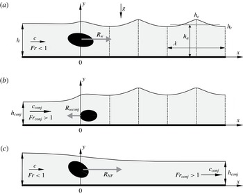
. The sketches of the subcritical and supercritical flows are shown in figure 3(a,b). It is worthwhile to stress that for both cases the waves far downstream are the same, but the bodies which generate these waves can differ in shape, size and their location with respect to the bottom.
Sketches of subcritical flows (a), supercritical flows (b) and hydraulic falls (c).

In paper 1, we have derived explicit analytical formulae (4.11), (4.12), (3.28b,c) for the solutions to system (5.9). In dimensionless form, the formulae can be rewritten as
 $$\begin{eqnarray}\displaystyle h=\frac{2R}{Fr^{2}+2},\quad c^{2}=Fr^{2}h, & & \displaystyle\end{eqnarray}$$
 $$\begin{eqnarray}\displaystyle h_{conj}=\unicode[STIX]{x1D705}h,\quad c_{conj}^{2}=\frac{Fr^{2}h}{\unicode[STIX]{x1D705}^{2}},\quad Fr_{conj}^{2}=\frac{Fr^{2}}{\unicode[STIX]{x1D705}^{3}}, & & \displaystyle\end{eqnarray}$$
where
 $$\begin{eqnarray}\displaystyle & \displaystyle \unicode[STIX]{x1D705}=\frac{Fr^{2}}{4}\left(1+\sqrt{1+\frac{8}{Fr^{2}}}\right)<1, & \displaystyle\end{eqnarray}$$
 $$\begin{eqnarray}\displaystyle \displaystyle Fr^{2}=6p\sin \left[\frac{1}{3}\arcsin \left(\frac{1}{p}\right)\right]-2<1,\quad p=\sqrt{\frac{8R^{3}}{27Q^{2}}}>1. & & \displaystyle\end{eqnarray}$$
5.1 Analytical formulae for
$R_{w}$
in the subcritical case

By making use of (5.8), (5.10), (5.12) and the expansions for
 $c_{a}^{2}$
,
 $c_{b}^{2}$
,
 $\unicode[STIX]{x1D6EC}$
,
 $V$
, the wave resistance for the subcritical case can be easily computed. Indeed, with the help of the identity (5.3) and equations (2.20), (3.3a
), (5.8) (5.10a
), we derive that
 $$\begin{eqnarray}\displaystyle R_{w}=3V-\frac{3}{2}\unicode[STIX]{x1D6FF}_{1}^{2}+h_{a}(1-Fr_{b}^{2})\unicode[STIX]{x1D6FF}_{1},\quad \unicode[STIX]{x1D6FF}_{1}=h_{a}\frac{Fr^{2}-Fr_{b}^{2}}{Fr^{2}+2},\quad p=\sqrt{\frac{(c_{b}^{2}+2h_{a})^{3}}{27c_{a}^{2}(\unicode[STIX]{x1D6EC}/2-h_{a})^{2}}}, & & \displaystyle \nonumber\\ \displaystyle & & \displaystyle\end{eqnarray}$$
where
 $Fr_{b}$
is the Froude number based on the mean depth
 $h_{a}$
and the root-mean-square bottom velocity
 $c_{b}$
:
 $$\begin{eqnarray}\displaystyle Fr_{b}=\frac{c_{b}}{\sqrt{h_{a}}}. & & \displaystyle\end{eqnarray}$$
Now, if the geometric parameters of the waves
 $a$
and
 $h_{a}$
are given, we compute the parameter
 $p$
by (5.13c
),
 $Fr^{2}$
by (5.12b
),
 $Fr_{b}$
by (5.14),
 $\unicode[STIX]{x1D6FF}_{1}$
by (5.13b
) and, finally,
 $R_{w}$
by (5.13a
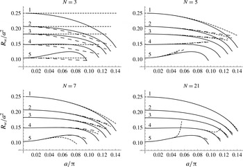
). In figure 4, we compare the results obtained by this analytical approach (long-dashed lines) with accurate numerical computations of
 $R_{w}$
carried out by the method of Maklakov (Reference Maklakov2002) (solid lines). The long-dashed lines are plotted only for
 $h_{a}<\infty$
, because for
 $h_{a}=\infty$
such a multistep technique of computing
 $R_{w}$
cannot be applied. As one can see, if the waves are not very steep, then even for small depths the results are in good agreement. The variable of the abscissa axes for the graphs of figure 4 is the waves steepness
 $a/\unicode[STIX]{x03C0}$
.
Comparison of analytical formulae with accurate numerical results for different
 $N$
and
 $h_{a}/2\unicode[STIX]{x03C0}=\infty$
, 0.3, 0.25, 0.2, 0.15 (1–5). Solid lines, numerical method of Maklakov (Reference Maklakov2002); long-dashed lines, analytical formulae (5.12)–(5.14); dashed lines, the direct asymptotic expansion of
 $R_{w}$
in powers of
 $a$
.

Application of formulae (5.12)–(5.14) for computing
 $R_{w}$
leaves some feeling of dissatisfaction caused by the necessity of taking several steps before getting the final result for
 $R_{w}$
. It seems that it would be better to obtain a direct asymptotic expansion of
 $R_{w}$
in powers of
 $a$
. A simple way to do this is to rewrite system (5.9) by the use of (2.20), (3.3a
) and (5.3) in the form
 $$\begin{eqnarray}\displaystyle c^{2}-2\unicode[STIX]{x1D6FF}_{1}=c_{b}^{2},\quad c(h_{a}-\unicode[STIX]{x1D6FF}_{1})=c_{a}(h_{a}-\unicode[STIX]{x1D6EC}/2). & & \displaystyle\end{eqnarray}$$
Excluding the unknown
 $c$
from system (5.15), we obtain the following cubic equation with respect to
 $\unicode[STIX]{x1D6FF}_{1}$
:
 $$\begin{eqnarray}\displaystyle (c_{b}^{2}+2\unicode[STIX]{x1D6FF}_{1})(h_{a}-\unicode[STIX]{x1D6FF}_{1})^{2}-c_{a}^{2}(h_{a}-\unicode[STIX]{x1D6EC}/2)^{2}=0, & & \displaystyle\end{eqnarray}$$
where the expansions for
 $c_{a}^{2}$
,
 $c_{b}^{2}$
and
 $\unicode[STIX]{x1D6EC}$
are known. To find an expansion for
 $\unicode[STIX]{x1D6FF}_{1}$
, we proceed in the same manner as in solving (4.8) or (4.11), namely, let
 $$\begin{eqnarray}\displaystyle \unicode[STIX]{x1D6FF}_{1}=\mathop{\sum }_{n=1}^{(N-1)/2}d_{2n}a^{2n}, & & \displaystyle\end{eqnarray}$$
where
 $d_{2n}$
are unknown coefficients. Substituting (5.17) into (5.16) and expanding the left-hand side of (5.16) in powers of
 $a$
up to the power
 $N$
inclusively, we obtain an
 $(N-1)$
-degree polynomial in even powers of
 $a$
with
 $(N-1)/2$
coefficients depending on the parameters
 $\unicode[STIX]{x1D700}=\exp (-2h_{a})$
,
 $h_{a}$
and the unknowns
 $d_{2n}$
. The coefficient at
 $a^{0}$
in this polynomial is zero. Equating the remainder coefficients to zero, we sequently find
 $d_{2},d_{4},\ldots ,\text{d}_{N-1}$
, which are now rational functions not only of
 $\unicode[STIX]{x1D700}$
but of
 $\unicode[STIX]{x1D700}$
and
 $h_{a}$
. After determining the expansion for
 $\unicode[STIX]{x1D6FF}_{1}$
, we find the expansion for
 $c$
by means of (5.15a
). Inserting the obtained values of
 $h=h_{a}-\unicode[STIX]{x1D6FF}_{1}$
and
 $c$
into (5.8), we find the expansion for the wave resistance
 $R_{w}$
. Another way to do the same is to insert
 $\unicode[STIX]{x1D6FF}_{1}$
directly into (5.13a
).
It needs to be emphasized that the values of
 $h$
and
 $c$
, found in such a manner, correspond to the subcritical solution to the system (5.9). This is a consequence of the representation (5.17). Indeed, if the amplitude
 $a\rightarrow 0$
, then we conclude from (5.17) that
 $\unicode[STIX]{x1D6FF}_{1}\rightarrow 0$
. In this case, as follows from (5.15a
),
 $c^{2}\rightarrow c_{b}^{2}$
. Taking into account that, when
 $a\rightarrow 0$
, the velocity
 $c_{a}$
satisfies the ordinary dispersion relation of the linear theory and
 $c_{a}=c_{b}$
, we find that
 $$\begin{eqnarray}\displaystyle c^{2}=\frac{1-\unicode[STIX]{x1D700}}{1+\unicode[STIX]{x1D700}}=\tanh h_{a}. & & \displaystyle\end{eqnarray}$$
This means that the Froude number
 $Fr=c/\sqrt{h_{a}}<1$
as
 $a\rightarrow 0$
. Hence, the representation (5.17) corresponds to the subcritical branch of solutions to system (5.9).
Formulae (B 6) and (B 7) of appendix B present these direct asymptotic expansions for
 $R_{w}$
and
 $\unicode[STIX]{x1D6FF}_{1}$
up to
 $a^{6}$
. If we take (B 6) only up to
 $a^{2}$
, then
 $$\begin{eqnarray}\displaystyle R_{w}=a^{2}\left[\frac{h_{a}\unicode[STIX]{x1D700}}{(\unicode[STIX]{x1D700}-1)(\unicode[STIX]{x1D700}+1)}+\frac{1}{4}\right]=\frac{a^{2}}{4}\left(1-\frac{2h_{a}}{\sinh 2h_{a}}\right), & & \displaystyle\end{eqnarray}$$
which exactly coincides with Kelvin’s formula for
 $R_{w}$
obtained from the linear wave theory (see Kelvin Reference Kelvin1887). Formula (B 6) generalizes the deep water fourth-order result by Duncan (Reference Duncan1983):
 $$\begin{eqnarray}\displaystyle R_{w}={\textstyle \frac{1}{4}}a^{2}-{\textstyle \frac{3}{8}}a^{4}, & & \displaystyle\end{eqnarray}$$
on to the case of finite depth up to
 $a^{6}$
.
We should remark that the mixture of
 $h_{a}$
and
 $\unicode[STIX]{x1D700}=\exp (-2h_{a})$
in the coefficients at
 $a^{n}$
makes the expansions for
 $R_{w}$
and
 $\unicode[STIX]{x1D6FF}_{1}$
much longer than the previous ones when the coefficients depend only on
 $\unicode[STIX]{x1D700}=\exp (-2h_{a})$
. For example, the expansion for
 $R_{w}$
at
 $N=21$
after conversion to LaTeX takes approximately 1300 kilobytes (compare with 75 kilobytes for
 $c_{a}^{2}$
), which corresponds to approximately several hundreds of journal pages.
In figure 4, the dashed lines are the results of computations of
 $R_{w}$
by its direct expansion in powers of
 $a$
. As one can see, for small depths (
 $h_{a}/2\unicode[STIX]{x03C0}=0.2,0.15$
) the results are worse than those obtained by the multistep method (long-dashed lines in figure 4). An explanation to this is the behaviour of the function
 $Fr^{2}(p)$
defined by formula (5.12b
). Indeed, the same direct asymptotic expansion of
 $R_{w}$
can be found by expanding the parameter
 $p$
, defined by (5.13c
), and after that, by expanding the function
 $Fr^{2}(p)$
in the Taylor series at the point
 $p_{0}$
, where
 $p_{0}$
is the value of
 $p$
at
 $a=0$
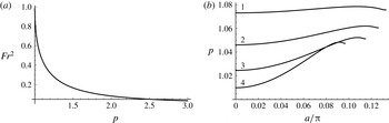
. The graph of the function
 $Fr^{2}(p)$
is shown in figure 5(a), and as one can see, near the point
 $p=1$
the derivatives of
 $Fr^{2}(p)$
are very large. As can be seen from figure 5(b), for
 $h_{a}/2\unicode[STIX]{x03C0}=0.2,0.15$
the values of
 $p_{0}$
is very close to unity. So it is difficult to expect a good result in the case of shallow water for the direct expansion of
 $R_{w}$
when we have such an unpleasant behaviour of
 $Fr^{2}(p)$
in the vicinity of
 $p=1$
.
Graph of the function
 $Fr^{2}(p)$
and the dependence of
 $p$
on
 $a/\unicode[STIX]{x03C0}$
for
 $h_{a}/2\unicode[STIX]{x03C0}=0.3$
, 0.25, 0.2, 0.15 (1–4), computed by the numerical method of Maklakov (Reference Maklakov2002).

The infinite depth case is also subcritical with the Froude number
 $Fr=0<1$
. For this case formulae (B 8)–(B 11) of appendix B present asymptotic expansions up to
 $a^{21}$
for
 $R_{w}$
,
 $c^{2}=c_{a}^{2}=c_{b}^{2}$
,
 $V$
and
 $T$
. Dallaston & McCue (Reference Dallaston and McCue2010) presented the formula for
 $c_{a}^{2}$
to
 $a^{14}$
(equation (11) of their paper). Comparison shows that all coefficients in their formula coincide with those of (B 9). In figure 4, the dashed lines labelled by number 1 demonstrate the results of computations of
 $R_{w}$
by formula (B 8) in comparison with accurate numerical computations by the method of Maklakov (Reference Maklakov2002) (solid lines). As one can see, the coincidence is not so bad, especially at
 $N=21$
.
5.2 Supercritical case
Free-surface flows with periodic downstream waves generated by a supercritical stream past an obstacle were discovered by Dias & Vanden-Broek (Reference Dias and Vanden-Broek2002), and further examples were computed by a number of authors (see, e.g. Dias & Vanden-Broek Reference Dias and Vanden-Broek2004; Binder, Vanden-Broek & Dias Reference Binder, Vanden-Broek and Dias2009). In figure 3(a,b), we demonstrate the sketches of subcritical and supercritical flows. For the supercritical case, the total pressure force exerted to the obstacle from the side of fluid we denote
 $R_{wconj}$
. As has been rigorously proved in paper 1, the values of
 $R_{w}$
(subcritical case) are always positive, but those of
 $R_{wconj}$
(supercritical case) are negative, which makes doubtful the physical realizability of flows in figure 3(b). Now we want to estimate the contribution of periodic waves to these negative values.
Consider the dimensionless form of the wave parameter introduced by Benjamin & Lighthill (Reference Benjamin and Lighthill1954), namely, the flow force
 $$\begin{eqnarray}\displaystyle S=\int _{0}^{\unicode[STIX]{x1D702}(x)}[u^{2}(x,y)+p]\,\text{d}y. & & \displaystyle\end{eqnarray}$$
It follows from the momentum equation that
 $$\begin{eqnarray}\displaystyle R_{w}=S_{u}(c,h)-S,\quad R_{wconj}=S_{u}(c_{conj},h_{conj})-S, & & \displaystyle\end{eqnarray}$$
where
 $S_{u}(c,h)$
is the flow force
 $S$
for a uniform stream with speed
 $c$
and depth
 $h$
. This leads to the formula
 $$\begin{eqnarray}\displaystyle R_{wconj}=R_{w}-[S_{u}(c,h)-S_{u}(c_{conj},h_{conj})]. & & \displaystyle\end{eqnarray}$$
The difference in square brackets is just the wave resistance for a so-called hydraulic fall: a waveless free-surface flow which is subcritical far upstream and supercritical far downstream (see Forbes Reference Forbes1988; Shen & Shen Reference Shen and Shen1990). The sketch of the hydraulic fall is shown in figure 3(c). We denote the wave resistance for such flows by
 $R_{HF}$
, its value being given by formula (3.28a) of paper 1. Thus, we come to the equations
 $$\begin{eqnarray}\displaystyle R_{wconj}=R_{w}-R_{HF},\quad R_{HF}=\frac{h^{2}}{2}\frac{(1-\unicode[STIX]{x1D705})^{3}}{1+\unicode[STIX]{x1D718}}, & & \displaystyle\end{eqnarray}$$
where
 $\unicode[STIX]{x1D705}=h_{conj}/h$
is defined by (5.12a
). Since
 $\unicode[STIX]{x1D705}<1$
, we have
 $R_{HF}>0$
, and according to the corollary to Proposition 1 of paper 1 (p. 299),
 $R_{HF}>R_{w}$
. So, the contribution of periodic wave train to the wave resistance is positive independently of the case, subcritical or supercritical. It is curious that all free flows shown in figure 3 are nonlinear, but their wave resistances are connected by the linear relationship (5.24a
).
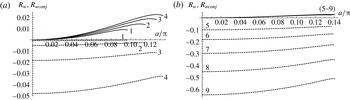
We do not give any expansions for the supercritical case due to our doubtfulness of its physical realizability, but for completeness we plot the graphs of
 $R_{w}$
(solid lines) together with its negative counterpart
 $R_{wconj}$
(dashed lines) in figure 6 for the depths
 $h_{a}/2\unicode[STIX]{x03C0}=0.15{-}0.55$
with a step of 0.05. The computations have been carried out by the method of the paper of Maklakov (Reference Maklakov2002). As one can see from the graphs, as the depths increase, the moduli of
 $R_{wconj}<0$
increase much faster than those of
 $R_{w}>0$
, creating a significant ‘wave thrust’.
Dependences of
 $R_{w}$
(solid lines) and
 $R_{wconj}$
(dashed lines) on the wave steepness
 $a/\unicode[STIX]{x03C0}$
for different depths
 $h_{a}/2\unicode[STIX]{x03C0}=0.15{-}0.55$
with a step of 0.05 (1–9). Computations have been carried out by the method of Maklakov (Reference Maklakov2002).

5.3 Comparison with Fenton’s fifth-order wave theory
Fenton (Reference Fenton1985) published a fifth-order wave theory based on the first Stokes method and presented explicit analytical expansions of wave properties in powers of
 $a$
with coefficients depending on
 $h_{a}$
. Since our expansions have the same structure but have been obtained by the second Stokes method, it is useful to compare the results of these independent calculations. Table 1 of Fenton’s work contains 22 coefficients which take part in formulae for the potential
 $\unicode[STIX]{x1D719}(x,y)$
, mean velocity
 $c_{a}$
, shape of free surface
 $\unicode[STIX]{x1D702}(x)$
, volume flux
 $Q$
and Bernoulli constant
 $R$
. These 22 coefficients have a rather complex structure and depend mainly on the parameter
 $S=\text{sech}(2h_{a})$
(do not confuse this
 $S$
with the flow force, defined by (5.21)). Taking into account that
 $$\begin{eqnarray}\displaystyle c_{a}=\sqrt{c_{a}^{2}},\quad Q=c_{a}(h_{a}-\unicode[STIX]{x1D6EC}/2),\quad R=c_{b}^{2}/2+h_{a} & & \displaystyle\end{eqnarray}$$
and using (B 1)–(B 3), we have obtained the corresponding expansions and compared them with those presented by Fenton. The results turn out to be in full coincidence.
To compare the mean potential energy
 $V$
, given by (B 4), we have used the explicit analytical expression for
 $\unicode[STIX]{x1D702}(x)$
of Fenton’s work. By means of (5.1a
), we have calculated
 $V$
to
 $a^{4}$
and compared the result with (B 4). Again, we have had the same full coincidence.
6 Concluding remarks
In this paper, for steady periodic gravity waves in water on finite depth, we have derived a quadratic system of equations with respect to the coefficients of the second Stokes method and developed an effective computer algorithm for solving the system. Making use of exact arithmetics and symbolic calculations, we have obtained explicit analytical expansions in powers of the wave amplitude
 $a$
for the wave resistance and other wave properties to
 $a^{21}$
. The coefficients of these expansions depend only on the mean wave depth
 $h_{a}$
.
To our regret, the expansions of order higher than seven are too long to be printed, and in appendix B to the paper we have presented the results only up to
 $a^{7}$
. Having taken a look at these formulae, the reader can easily imagine the length of expansions of order
 $a^{9}$
and higher. In spite of this evident deficiency, the formulae have also an important advantage: because even their LaTeX forms for printout have been generated by computer, they cannot contain any typos or calculational errors. On the other hand, these long analytical formulae, which sometimes take several hundreds of journal pages, are a logical consequence of accurate application of the famous analytical Stokes approach.
A usual way to enhance the convergence of the high-order Stokes expansions is the use of Padé approximants. However, this approach is effective when the Stokes coefficients are numbers, decimal as in Schwartz (Reference Schwartz1974) and Cokelet (Reference Cokelet1977) or rational as in Dallaston & McCue (Reference Dallaston and McCue2010). In our case, the coefficients are rational functions of
 $\unicode[STIX]{x1D700}=\exp (-2h_{a})$
(at best) or a mixture of
 $h_{a}$
and
 $\unicode[STIX]{x1D700}$
(at worst). By specifying
 $a$
and
 $h_{a}$
, we are able to compute these coefficients and represent them as numbers with any quantity of decimal places, but then all analyticity of our approach will be lost and we return to the previous investigations.
We have compared our asymptotic expansions with those obtained by the fifth-order theory of Fenton (Reference Fenton1985) and found that the results are in full coincidence. Comparison also has been made with the results obtained in paper 1, where the waves resistance
 $R_{w}$
was computed by the accurate numerical method of the work by Maklakov (Reference Maklakov2002). The conclusion is as follows: analytical expansions to
 $a^{7}$
can be applied if the depth-to-wavelength ratio is not less than 0.15 and the wave amplitude is approximately 60 % of its limiting value.
All expansions used in the paper are stored in the supplementary materials and are available at https://doi.org/10.1017/jfm.2017.62 in the form of Mathematica expressions. The order of the stored expressions is 21. The materials contain the file ‘Instruction.nb’, which explains how to use the stored information.
Acknowledgements
The work was supported by the Russian Science Foundation, project no. 14-19-01633. The authors are very grateful to the referees for valuable comments which were very constructive and allowed us to improve the manuscript substantially.
Supplementary materials
Supplementary materials are available at https://doi.org/10.1017/jfm.2017.62.
Appendix A. Proofs of formulae (3.3), (3.4) and (3.9)
First, we prove formula (3.3a ). In terms of the Stokes coefficients the mean depth
 $$\begin{eqnarray}\displaystyle h_{a}=\frac{1}{2\unicode[STIX]{x03C0}}\int _{0}^{2\unicode[STIX]{x03C0}}\left(-\log r_{0}+\mathop{\sum }_{n=1}^{\infty }\unicode[STIX]{x1D6FD}_{n}y_{n}\cos n\unicode[STIX]{x1D6FE}\right)\left(1+\mathop{\sum }_{n=1}^{\infty }n\unicode[STIX]{x1D6FC}_{n}y_{n}\cos n\unicode[STIX]{x1D6FE}\right)\,\text{d}\unicode[STIX]{x1D6FE}. & & \displaystyle\end{eqnarray}$$
Opening the brackets and integrating leads to (3.3a ) and (3.4a ).
Now, we prove (3.3b
). For the root-mean-squared depth
 $H_{a}$
we have
 $$\begin{eqnarray}\displaystyle H_{a}^{2}=\frac{1}{2\unicode[STIX]{x03C0}}\int _{0}^{2\unicode[STIX]{x03C0}}\left(-\log r_{0}+\mathop{\sum }_{n=1}^{\infty }\unicode[STIX]{x1D6FD}_{n}y_{n}\cos n\unicode[STIX]{x1D6FE}\right)^{2}\left(1+\mathop{\sum }_{n=1}^{\infty }n\unicode[STIX]{x1D6FC}_{n}y_{n}\cos n\unicode[STIX]{x1D6FE}\right)\,\text{d}\unicode[STIX]{x1D6FE}. & & \displaystyle\end{eqnarray}$$
Again, we open the brackets and integrate to obtain
 $$\begin{eqnarray}\displaystyle H_{a}^{2}=\log ^{2}r_{0}-\unicode[STIX]{x1D6EC}\log r_{0}+\frac{\unicode[STIX]{x1D6EC}_{1}}{2}+\frac{G}{2}, & & \displaystyle\end{eqnarray}$$
where
 $\unicode[STIX]{x1D6EC}_{1}$
is defined by (3.4b
), and
 $$\begin{eqnarray}\displaystyle G=\frac{1}{\unicode[STIX]{x03C0}}\int _{0}^{2\unicode[STIX]{x03C0}}\underbrace{\left(\mathop{\sum }_{n=1}^{\infty }\unicode[STIX]{x1D6FD}_{n}y_{n}\cos n\unicode[STIX]{x1D6FE}\right)^{2}}_{f(\unicode[STIX]{x1D6FE})}\left(\mathop{\sum }_{n=1}^{\infty }n\unicode[STIX]{x1D6FC}_{n}y_{n}\cos n\unicode[STIX]{x1D6FE}\right)\,\text{d}\unicode[STIX]{x1D6FE}. & & \displaystyle\end{eqnarray}$$
The first factor of the integrand in (A 4) we denote by
 $f(\unicode[STIX]{x1D6FE})$
. Then
 $$\begin{eqnarray}\displaystyle f(\unicode[STIX]{x1D6FE}) & = & \displaystyle \left(\mathop{\sum }_{n=1}^{\infty }\unicode[STIX]{x1D6FD}_{n}y_{n}\cos n\unicode[STIX]{x1D6FE}\right)\left(\mathop{\sum }_{m=1}^{\infty }\unicode[STIX]{x1D6FD}_{m}y_{m}\cos m\unicode[STIX]{x1D6FE}\right)\nonumber\\ \displaystyle & = & \displaystyle \frac{1}{2}\mathop{\sum }_{n=1}^{\infty }\unicode[STIX]{x1D6FD}_{n}y_{n}\mathop{\sum }_{m=1}^{\infty }\unicode[STIX]{x1D6FD}_{m}y_{m}[\cos (n+m)\unicode[STIX]{x1D6FE}+\cos (n-m)\unicode[STIX]{x1D6FE}].\end{eqnarray}$$
Representing
 $f(\unicode[STIX]{x1D6FE})$
as a Fourier series in cosine, we obtain
 $$\begin{eqnarray}\displaystyle f(\unicode[STIX]{x1D6FE}) & = & \displaystyle \frac{\unicode[STIX]{x1D6EC}_{1}}{2}+\frac{1}{2}\mathop{\sum }_{k=1}^{\infty }\cos k\unicode[STIX]{x1D6FE}\left(\mathop{\sum }_{m+n=k}\unicode[STIX]{x1D6FD}_{n}\unicode[STIX]{x1D6FD}_{m}y_{n}y_{m}+\mathop{\sum }_{n-m=k}\unicode[STIX]{x1D6FD}_{n}\unicode[STIX]{x1D6FD}_{m}y_{n}y_{m}\right.\nonumber\\ \displaystyle & & \displaystyle \left.+\,\mathop{\sum }_{m-n=k}\unicode[STIX]{x1D6FD}_{n}\unicode[STIX]{x1D6FD}_{m}y_{n}y_{m}\right),\quad m,n=1,2,3,\ldots ,\end{eqnarray}$$
where for the sums in brackets, the lower equalities define the indexes which take part in forming the summands. Inserting this expression for
 $f(\unicode[STIX]{x1D6FE})$
in (A 4) and taking into account that
 $$\begin{eqnarray}\displaystyle \mathop{\sum }_{n-m=k}\unicode[STIX]{x1D6FD}_{n}\unicode[STIX]{x1D6FD}_{m}y_{n}y_{m}=\mathop{\sum }_{m-n=k}\unicode[STIX]{x1D6FD}_{n}\unicode[STIX]{x1D6FD}_{m}y_{n}y_{m},\quad k,m,n=1,2,3,\ldots , & & \displaystyle\end{eqnarray}$$
after integration we get
 $$\begin{eqnarray}\displaystyle G=\mathop{\sum }_{k=1}^{\infty }k\unicode[STIX]{x1D6FC}_{k}y_{k}\left(\frac{1}{2}\mathop{\sum }_{m+n=k}\unicode[STIX]{x1D6FD}_{n}\unicode[STIX]{x1D6FD}_{m}y_{n}y_{m}+A\right), & & \displaystyle\end{eqnarray}$$
where
 $$\begin{eqnarray}\displaystyle A=\mathop{\sum }_{k=1}^{\infty }k\unicode[STIX]{x1D6FC}_{k}y_{k}\mathop{\sum }_{n-m=k}\unicode[STIX]{x1D6FD}_{n}\unicode[STIX]{x1D6FD}_{m}y_{n}y_{m}. & & \displaystyle\end{eqnarray}$$
In the sum
 $A$
, the index
 $n$
changes from 1 to infinity, and at fixed
 $n$
we have
 $m+k=n$
. Now, we reorder the summation by forming the outer sum over
 $n$
. This gives
 $$\begin{eqnarray}\displaystyle A=\mathop{\sum }_{n=1}^{\infty }\unicode[STIX]{x1D6FD}_{n}y_{n}\mathop{\sum }_{m+k=n}k\unicode[STIX]{x1D6FC}_{k}\unicode[STIX]{x1D6FD}_{m}y_{k}y_{m}=\mathop{\sum }_{k=1}^{\infty }\unicode[STIX]{x1D6FD}_{k}y_{k}\mathop{\sum }_{m+n=k}n\unicode[STIX]{x1D6FC}_{n}\unicode[STIX]{x1D6FD}_{m}y_{n}y_{m}, & & \displaystyle\end{eqnarray}$$
where to obtain the last equality we swap indexes
 $k$
and
 $n$
. Inserting this expression for
 $A$
into (A 8) and taking into account that
 $k=m+n$
, we infer
 $$\begin{eqnarray}\displaystyle G=\mathop{\sum }_{k=2}^{\infty }y_{k}\mathop{\sum }_{m+n=k}\unicode[STIX]{x1D70E}_{m,n}y_{m}y_{n}, & & \displaystyle\end{eqnarray}$$
where
 $$\begin{eqnarray}\displaystyle \unicode[STIX]{x1D70E}_{m,n}={\textstyle \frac{1}{2}}(m+n)\unicode[STIX]{x1D6FC}_{m+n}\unicode[STIX]{x1D6FD}_{m}\unicode[STIX]{x1D6FD}_{n}+n\unicode[STIX]{x1D6FC}_{n}\unicode[STIX]{x1D6FD}_{m+n}\unicode[STIX]{x1D6FD}_{m}. & & \displaystyle\end{eqnarray}$$
Here, the summation starts with
 $k=2$
since
 $m+n=k\geqslant 2$
. To make the coefficients in the inner sum symmetric with respect to
 $m$
and
 $n$
, we introduce
 $$\begin{eqnarray}\displaystyle \unicode[STIX]{x1D6E4}_{m,n}=(\unicode[STIX]{x1D70E}_{m,n}+\unicode[STIX]{x1D70E}_{n,m})/2. & & \displaystyle\end{eqnarray}$$
Then
 $$\begin{eqnarray}\displaystyle G=\mathop{\sum }_{k=2}^{\infty }y_{k}\mathop{\sum }_{m+n=k}\unicode[STIX]{x1D6E4}_{m,n}y_{m}y_{n}=\mathop{\sum }_{k=2}^{\infty }y_{k}\mathop{\sum }_{n=1}^{k-1}\unicode[STIX]{x1D6E4}_{k-n,n}y_{n}y_{k-n},\quad \unicode[STIX]{x1D6E4}_{m,n}=\unicode[STIX]{x1D6E4}_{n,m}. & & \displaystyle\end{eqnarray}$$
After a little algebra, it is possible to demonstrate that
 $\unicode[STIX]{x1D6E4}_{m,n}$
is defined by equation (3.5b
). This finalizes the proof of formulae (3.3b
) and (3.4c
). It is to be noted that reordering the summation in (A 9) is the key point for obtaining a compact expression for
 $G$
.
Now we prove the equality (3.9). We denote
 $$\begin{eqnarray}\displaystyle C_{k}=\mathop{\sum }_{m=1}^{k-1}\unicode[STIX]{x1D6E4}_{k-m,m}y_{m}y_{k-m},\quad k=2,3,4,\ldots & & \displaystyle\end{eqnarray}$$
It is easy to see that
 $$\begin{eqnarray}\displaystyle \frac{\unicode[STIX]{x2202}C_{k}}{\unicode[STIX]{x2202}y_{n}}=\left\{\begin{array}{@{}ll@{}}0 & \text{if }n>k-1\Leftrightarrow k<n+1,\\ 2\unicode[STIX]{x1D6E4}_{k-n,n}y_{k-n} & \text{if }n\leqslant k-1\Leftrightarrow k\geqslant n+1.\end{array}\right. & & \displaystyle\end{eqnarray}$$
Now,
 $$\begin{eqnarray}\displaystyle \frac{\unicode[STIX]{x2202}G}{\unicode[STIX]{x2202}y_{n}}=\mathop{\sum }_{m=1}^{n-1}\unicode[STIX]{x1D6E4}_{n-m,m}y_{m}y_{n-m}+2\mathop{\sum }_{k=n+1}^{\infty }\unicode[STIX]{x1D6E4}_{k-n,n}y_{k}y_{k-n}. & & \displaystyle\end{eqnarray}$$
If we put in the second sum of (A 17) that
 $k-n=m$
, we come to (3.9). It is worth noting that if
 $n=1$
, then the first sum on the right-hand side of (3.9) vanishes.
Appendix B. Eleven asymptotical expansions for wave properties
The expansions below have been generated and converted into LaTeX by computer. For this reason, they cannot contain any typos or calculational errors. A principle of choosing the order of expansions has been very simple: we present an expansion only if any fraction in it takes not more than one line of the journal page. The notation
 $P_{n}(x_{1},x_{2},\ldots ,x_{[n/2]+1})$
is that for palindromic polynomials of degree
 $n$
in powers of
 $\unicode[STIX]{x1D700}$
, the arguments being the first half of coefficients.
B.1 Expansions for finite depth with coefficients depending only on
$\unicode[STIX]{x1D700}=\exp (-2h_{a})$

 $$\begin{eqnarray}\displaystyle \displaystyle c_{a}^{2} & = & \displaystyle \displaystyle -\frac{a^{6}P_{20}(9,72,-2767,-2614,114687,491970,1155180,2005398,2928016,3608614,3897270)}{6(\unicode[STIX]{x1D700}-1)^{15}(\unicode[STIX]{x1D700}+1)P_{2}(2,1)P_{2}(3,4)}\nonumber\\ \displaystyle & & \displaystyle \displaystyle +\,\frac{a^{4}P_{10}(-1,-7,39,400,166,426)}{2(\unicode[STIX]{x1D700}-1)^{9}(\unicode[STIX]{x1D700}+1)}-\frac{a^{2}P_{4}(1,0,16)}{(\unicode[STIX]{x1D700}-1)^{3}(\unicode[STIX]{x1D700}+1)}-\frac{\unicode[STIX]{x1D700}-1}{\unicode[STIX]{x1D700}+1},\end{eqnarray}$$
 $$\begin{eqnarray}\displaystyle \displaystyle c_{b}^{2} & = & \displaystyle \displaystyle -\frac{a^{6}P_{20}(9,-132,-1954,7640,127743,496104,1139076,2002512,2912560,3620356,3886572)}{6(\unicode[STIX]{x1D700}-1)^{15}(\unicode[STIX]{x1D700}+1)P_{2}(2,1)P_{2}(3,4)}\nonumber\\ \displaystyle & & \displaystyle \displaystyle +\,\frac{a^{4}P_{10}(-1,-3,71,296,302,290)}{2(\unicode[STIX]{x1D700}-1)^{9}(\unicode[STIX]{x1D700}+1)}-\frac{a^{2}P_{4}(1,2,12)}{(\unicode[STIX]{x1D700}-1)^{3}(\unicode[STIX]{x1D700}+1)}-\frac{\unicode[STIX]{x1D700}-1}{\unicode[STIX]{x1D700}+1},\end{eqnarray}$$
 $$\begin{eqnarray}\displaystyle \displaystyle \unicode[STIX]{x1D6EC} & = & \displaystyle \displaystyle -\frac{a^{6}(\unicode[STIX]{x1D700}+1)P_{16}(-13,-56,671,2866,7542,10250,16461,16724,20710)}{2(\unicode[STIX]{x1D700}-1)^{13}P_{2}(2,1)P_{2}(3,4)}\nonumber\\ \displaystyle & & \displaystyle \displaystyle +\,\frac{a^{4}(\unicode[STIX]{x1D700}+1)P_{2}(1,-1)P_{4}(1,2,12)}{(\unicode[STIX]{x1D700}-1)^{7}}-\frac{a^{2}(\unicode[STIX]{x1D700}+1)}{\unicode[STIX]{x1D700}-1},\end{eqnarray}$$
 $$\begin{eqnarray}\displaystyle V & = & \displaystyle \displaystyle \frac{a^{6}P_{16}(-19,-49,376,2061,5840,11203,16032,19281,20150)}{8(\unicode[STIX]{x1D700}-1)^{12}P_{2}(2,1)P_{2}(3,4)}\nonumber\\ \displaystyle & & \displaystyle \displaystyle -\,\frac{a^{4}P_{2}(1,4)P_{4}(1,0,4)}{8(\unicode[STIX]{x1D700}-1)^{6}}+\frac{a^{2}}{4},\end{eqnarray}$$
 $$\begin{eqnarray}\displaystyle T_{c_{a}} & = & \displaystyle \displaystyle \frac{a^{6}P_{16}(-19,-25,108,473,4656,10679,17532,20313,22166)}{8(\unicode[STIX]{x1D700}-1)^{12}P_{2}(2,1)P_{2}(3,4)}\nonumber\\ \displaystyle & & \displaystyle \displaystyle -\,\frac{3a^{4}\unicode[STIX]{x1D700}P_{4}(1,-2,8)}{4(\unicode[STIX]{x1D700}-1)^{6}}+\frac{a^{2}}{4},\end{eqnarray}$$
B.2 Expansions for finite depth with coefficients which depend on a mixture of
$\unicode[STIX]{x1D700}=\exp (-2h_{a})$
and
$h_{a}$


 $$\begin{eqnarray}\displaystyle \displaystyle R_{w} & = & \displaystyle \displaystyle a^{6}\left[\frac{h_{a}^{4}\unicode[STIX]{x1D700}(\unicode[STIX]{x1D700}+1)^{2}P_{16}(-68,135,3756,11729,21080,25063,28084,25953,27736)}{4(\unicode[STIX]{x1D700}-1)^{13}P_{2}(2,1)P_{2}(3,4)(h_{a}\unicode[STIX]{x1D700}+h_{a}+\unicode[STIX]{x1D700}-1)^{3}}\right.\nonumber\\ \displaystyle & & \displaystyle \displaystyle +\,\frac{h_{a}^{3}(\unicode[STIX]{x1D700}+1)P_{18}(-19,-543,1461,29124,91280,158624,198664,220060,223558,229182)}{8(\unicode[STIX]{x1D700}-1)^{12}P_{2}(2,1)P_{2}(3,4)(h_{a}\unicode[STIX]{x1D700}+h_{a}+\unicode[STIX]{x1D700}-1)^{3}}\nonumber\\ \displaystyle & & \displaystyle \displaystyle +\,\frac{h_{a}^{2}P_{18}(-51,-754,3161,42450,131460,225936,288948,329998,351778,364548)}{8(\unicode[STIX]{x1D700}-1)^{11}P_{2}(2,1)P_{2}(3,4)(h_{a}\unicode[STIX]{x1D700}+h_{a}+\unicode[STIX]{x1D700}-1)^{3}}\nonumber\\ \displaystyle & & \displaystyle \displaystyle +\,\frac{h_{a}P_{18}(-39,-406,3052,27914,82337,142176,187347,221974,244551,255788)}{8(\unicode[STIX]{x1D700}-1)^{10}(\unicode[STIX]{x1D700}+1)P_{2}(2,1)P_{2}(3,4)(h_{a}\unicode[STIX]{x1D700}+h_{a}+\unicode[STIX]{x1D700}-1)^{3}}\nonumber\\ \displaystyle & & \displaystyle \left.\displaystyle +\,\frac{P_{16}(-8,-67,2264,9339,16832,23481,28248,32623,33776)}{16(\unicode[STIX]{x1D700}-1)^{9}P_{2}(2,1)P_{2}(3,4)(h_{a}\unicode[STIX]{x1D700}+h_{a}+\unicode[STIX]{x1D700}-1)^{3}}\right]\nonumber\\ \displaystyle & & \displaystyle \displaystyle +\,a^{4}\left[-\frac{h_{a}^{2}\unicode[STIX]{x1D700}P_{6}(1,10,-7,10)}{(\unicode[STIX]{x1D700}-1)^{7}(h_{a}\unicode[STIX]{x1D700}+h_{a}+\unicode[STIX]{x1D700}-1)}-\frac{h_{a}P_{8}(3,14,118,-10,38)}{8(\unicode[STIX]{x1D700}-1)^{6}(\unicode[STIX]{x1D700}+1)(h_{a}\unicode[STIX]{x1D700}+h_{a}+\unicode[STIX]{x1D700}-1)}\right.\nonumber\\ \displaystyle & & \displaystyle \left.\displaystyle -\,\frac{P_{6}(2,1,11,-10)}{4(\unicode[STIX]{x1D700}-1)^{5}(h_{a}\unicode[STIX]{x1D700}+h_{a}+\unicode[STIX]{x1D700}-1)}\right]+a^{2}\displaystyle \left[\frac{h_{a}\unicode[STIX]{x1D700}}{(\unicode[STIX]{x1D700}-1)(\unicode[STIX]{x1D700}+1)}+\frac{1}{4}\right],\end{eqnarray}$$
 $$\begin{eqnarray}\displaystyle \displaystyle \unicode[STIX]{x1D6FF}_{1} & = & \displaystyle \displaystyle a^{6}\left[\frac{h_{a}^{5}\unicode[STIX]{x1D700}(\unicode[STIX]{x1D700}+1)^{4}P_{16}(-68,135,3756,11729,21080,25063,28084,25953,27736)}{4(\unicode[STIX]{x1D700}-1)^{13}P_{2}(2,1)P_{2}(3,4)(h_{a}\unicode[STIX]{x1D700}+h_{a}+\unicode[STIX]{x1D700}-1)^{5}}\right.\nonumber\\ \displaystyle & & \displaystyle \displaystyle +\,\frac{h_{a}^{4}(\unicode[STIX]{x1D700}+1)^{3}P_{18}(19,-197,655,15018,49952,61276,65136,29054,33950,8674)}{4(\unicode[STIX]{x1D700}-1)^{12}P_{2}(2,1)P_{2}(3,4)(h_{a}\unicode[STIX]{x1D700}+h_{a}+\unicode[STIX]{x1D700}-1)^{5}}\nonumber\\ \displaystyle & & \displaystyle \displaystyle +\,\frac{h_{a}^{3}(\unicode[STIX]{x1D700}+1)^{2}P_{18}(170,-75,2588,38862,127206,80752,-56918,-244606,-295670,-341418)}{8(\unicode[STIX]{x1D700}-1)^{11}P_{2}(2,1)P_{2}(3,4)(h_{a}\unicode[STIX]{x1D700}+h_{a}+\unicode[STIX]{x1D700}-1)^{5}}\nonumber\\ \displaystyle & & \displaystyle \displaystyle +\,\frac{h_{a}^{2}(\unicode[STIX]{x1D700}+1)P_{18}(270,709,960,11402,18362,-112344,-354978,-581050,-695942,-721978)}{8(\unicode[STIX]{x1D700}-1)^{10}P_{2}(2,1)P_{2}(3,4)(h_{a}\unicode[STIX]{x1D700}+h_{a}+\unicode[STIX]{x1D700}-1)^{5}}\nonumber\\ \displaystyle & & \displaystyle \displaystyle -\,\frac{h_{a}P_{18}(-140,-664,2335,14944,56641,163208,316859,452336,532369,553024)}{8(\unicode[STIX]{x1D700}-1)^{9}P_{2}(2,1)P_{2}(3,4)(h_{a}\unicode[STIX]{x1D700}+h_{a}+\unicode[STIX]{x1D700}-1)^{5}}\nonumber\\ \displaystyle & & \displaystyle \left.\displaystyle -\,\frac{(\unicode[STIX]{x1D700}+1)P_{16}(50,-61,3188,10533,27616,44927,63932,70649,76732)}{16(\unicode[STIX]{x1D700}-1)^{8}P_{2}(2,1)P_{2}(3,4)(h_{a}\unicode[STIX]{x1D700}+h_{a}+\unicode[STIX]{x1D700}-1)^{5}}\right]\nonumber\\ \displaystyle & & \displaystyle \displaystyle +\,a^{4}\left[-\frac{h_{a}^{3}\unicode[STIX]{x1D700}(\unicode[STIX]{x1D700}+1)^{2}P_{6}(1,10,-7,10)}{(\unicode[STIX]{x1D700}-1)^{7}(h_{a}\unicode[STIX]{x1D700}+h_{a}+\unicode[STIX]{x1D700}-1)^{3}}-\frac{3h_{a}^{2}\unicode[STIX]{x1D700}(\unicode[STIX]{x1D700}+1)P_{4}(1,14,24)}{2(\unicode[STIX]{x1D700}-1)^{4}(h_{a}\unicode[STIX]{x1D700}+h_{a}+\unicode[STIX]{x1D700}-1)^{3}}\right.\nonumber\\ \displaystyle & & \displaystyle \left.\displaystyle +\,\frac{3h_{a}P_{8}(1,0,0,32,78)}{8(\unicode[STIX]{x1D700}-1)^{5}(h_{a}\unicode[STIX]{x1D700}+h_{a}+\unicode[STIX]{x1D700}-1)^{3}}+\frac{(\unicode[STIX]{x1D700}+1)P_{6}(3,2,13,0)}{4(\unicode[STIX]{x1D700}-1)^{4}(h_{a}\unicode[STIX]{x1D700}+h_{a}+\unicode[STIX]{x1D700}-1)^{3}}\right]\nonumber\\ \displaystyle & & \displaystyle \displaystyle +\,a^{2}\left[\frac{h_{a}\unicode[STIX]{x1D700}}{(\unicode[STIX]{x1D700}-1)(h_{a}\unicode[STIX]{x1D700}+h_{a}+\unicode[STIX]{x1D700}-1)}-\frac{\unicode[STIX]{x1D700}+1}{2(h_{a}\unicode[STIX]{x1D700}+h_{a}+\unicode[STIX]{x1D700}-1)}\right].\end{eqnarray}$$
B.3 Expansions for infinite depth
 $$\begin{eqnarray}\displaystyle \displaystyle R_{w} & = & \displaystyle \displaystyle \frac{a^{2}}{4}-\frac{3a^{4}}{8}-\frac{19a^{6}}{48}-\frac{2597a^{8}}{2880}-\frac{559733a^{10}}{201600}-\frac{9766021889a^{12}}{1016064000}\nonumber\\ \displaystyle & & \displaystyle -\,\displaystyle \frac{1007540062126771a^{14}}{28165294080000}-\frac{1417604531750289802727a^{16}}{10149645374668800000}\nonumber\\ \displaystyle & & \displaystyle -\,\displaystyle \frac{2063615976870165517551724279a^{18}}{3657526207215648768000000}\nonumber\\ \displaystyle & & \displaystyle -\,\displaystyle \frac{52376619112355935298282434064177671a^{20}}{22406444448547930230620160000000},\end{eqnarray}$$
 $$\begin{eqnarray}\displaystyle \displaystyle c^{2}=c_{a}^{2}=c_{b}^{2} & = & \displaystyle \displaystyle 1+a^{2}+\frac{a^{4}}{2}+\frac{a^{6}}{4}-\frac{22a^{8}}{45}-\frac{115069a^{10}}{25200}-\frac{6379033039a^{12}}{254016000}\nonumber\\ \displaystyle & & \displaystyle \displaystyle -\,\frac{875167353344611a^{14}}{7041323520000}-\frac{1509490905485738054687a^{16}}{2537411343667200000}\nonumber\\ \displaystyle & & \displaystyle \displaystyle -\,\frac{2573919846675736709873575159a^{18}}{914381551803912192000000}\nonumber\\ \displaystyle & & \displaystyle \displaystyle -\,\frac{74381757900412915700748130785581431a^{20}}{5601611112136982557655040000000},\end{eqnarray}$$
 $$\begin{eqnarray}\displaystyle V & = & \displaystyle \displaystyle \frac{a^{2}}{4}-\frac{a^{4}}{8}-\frac{19a^{6}}{48}-\frac{3077a^{8}}{2880}-\frac{702113a^{10}}{201600}-\frac{12793118129a^{12}}{1016064000}\nonumber\\ \displaystyle & & \displaystyle \displaystyle -\,\frac{1366685377769731a^{14}}{28165294080000}-\frac{1981974995491975924247a^{16}}{10149645374668800000}\nonumber\\ \displaystyle & & \displaystyle \displaystyle -\,\frac{2965179893909091084219806119a^{18}}{3657526207215648768000000}\nonumber\\ \displaystyle & & \displaystyle \displaystyle -\,\frac{77199563300878281492652707790632631a^{20}}{22406444448547930230620160000000},\end{eqnarray}$$
 $$\begin{eqnarray}\displaystyle T & = & \displaystyle \displaystyle \frac{a^{2}}{4}-\frac{19a^{6}}{48}-\frac{3317a^{8}}{2880}-\frac{773303a^{10}}{201600}-\frac{14306666249a^{12}}{1016064000}\nonumber\\ \displaystyle & & \displaystyle \displaystyle -\,\frac{1546258035591211a^{14}}{28165294080000}-\frac{2264160227362818985007a^{16}}{10149645374668800000}\nonumber\\ \displaystyle & & \displaystyle \displaystyle -\,\frac{3415961852428553867553847039a^{18}}{3657526207215648768000000}\nonumber\\ \displaystyle & & \displaystyle \displaystyle -\,\frac{89611035395139454589837844653860111a^{20}}{22406444448547930230620160000000}.\end{eqnarray}$$