1 Introduction
Rayleigh–Bénard (RB) convection is a paradigm in hydrodynamic stability and pattern formation studies (Chandrasekhar Reference Chandrasekhar1961; Normand, Pomeau & Velarde Reference Normand, Pomeau and Velarde1977; Cross & Hohenberg Reference Cross and Hohenberg1993; Bodenschatz, Pesch & Ahlers Reference Bodenschatz, Pesch and Ahlers2000). It is commonly investigated under the Oberbeck–Boussinesq (OB) approximation, assuming an incompressible flow and constant fluid properties except for a linear relationship between density and temperature in the buoyancy term (Oberbeck Reference Oberbeck1879; Boussinesq Reference Boussinesq1903).
However, non-Oberbeck–Boussinesq (NOB) effects must be taken into account under some practical circumstances, such as the thermal insulation systems in nuclear reactors, where the typical temperature difference is of the order of several hundred kelvins. When convection occurs with such a large temperature difference, the variations of fluid properties or flow compressibility are so significant that OB approximation is no longer valid (Gray & Giorgini Reference Gray and Giorgini1976; Paolucci Reference Paolucci1982).
It is well known that NOB effects will break the reflection symmetry of an RB system about the horizontal mid-plane and have strong influences on instabilities and flow transitions, as shown in previous studies. A sizable literature is devoted to the study of NOB influences on pattern-forming instabilities of spatially extended systems. Busse (Reference Busse1967) theoretically investigated the NOB influences due to temperature dependence of material properties on the dominant RB convection pattern near convection onset. It was found that NOB convection appears in the form of a hexagonal pattern at lower Rayleigh number, and transition to a roll pattern occurs at higher Rayleigh number. Several experiments have been reported to further explore these NOB influences (Ahlers Reference Ahlers1980; Ciliberto, Pampaloni & Perez-Garcia Reference Ciliberto, Pampaloni and Perez-Garcia1988; Ciliberto et al. Reference Ciliberto, Coullet, Lega, Pampaloni and Perez-Garcia1990; Bodenschatz et al. Reference Bodenschatz, de Bruyn, Ahlers and Cannell1991; Pampaloni et al. Reference Pampaloni, Perez-Garcia, Albavetti and Ciliberto1992). We refer to Bodenschatz et al. (Reference Bodenschatz, Pesch and Ahlers2000) for a review. Recently Ahlers et al. (Reference Ahlers, Dressel, Oh and Pesch2010) experimentally and theoretically studied the strong NOB effects near convection onset using sulfur hexafluoride near its gas–liquid critical point. The NOB effects were divided into two disjunct parts, one preserving the reflection symmetry of the system about the horizontal mid-plane and the other breaking that symmetry.
There have been several studies devoted to the NOB effects in two-dimensional RB convection. By numerically solving the low-Mach-number equations, Paolucci & Chenoweth (Reference Paolucci and Chenoweth1987) investigated the instability of convection onset and heat transfer of the RB system of perfect gas in a two-dimensional cavity of aspect ratio 20. Corrections of critical Rayleigh number and Nusselt number were found to depend to the second order on the departures from the OB approximation. Fröhlich, Laure & Peyret (Reference Fröhlich, Laure and Peyret1992) studied the NOB convection of perfect gas in a two-dimensional periodic system via linear and weakly nonlinear stability analysis and direct numerical simulation (DNS) of the low-Mach-number equations. Qualitative change of the bifurcation nature of convection onset was observed and the transition to convection rolls was found to be subcritical with strong NOB effects.
The NOB effects in other convection problems have also been studied. Suslov & Paolucci (Reference Suslov and Paolucci1995) studied the linear stability of fully developed mixed convection in a differentially heated vertical channel. New unstable modes due entirely to NOB effects were found. Weakly nonlinear analysis of NOB convection in a tall vertical enclosure was performed in Suslov & Paolucci (Reference Suslov and Paolucci1997). Bifurcation characteristics of shear- and buoyancy-driven instabilities and their interactions were investigated. The NOB influences on weakly nonlinear instability of mixed convection in an open system were also studied (Suslov & Paolucci Reference Suslov and Paolucci1999a ,Reference Suslov and Paolucci b ), and bifurcations and mean flow characteristics were investigated in detail. Recently the NOB influences on large-scale dynamics and heat transport of high-Rayleigh-number convection have also received considerable attention (Ahlers et al. Reference Ahlers, Brown, Araujo, Funfschilling, Grossmann and Lohse2006; Sugiyama et al. Reference Sugiyama, Calzavarini, Grossmann and Lohse2007; Ahlers, Grossmann & Lohse Reference Ahlers, Grossmann and Lohse2009; Chillà & Schumacher Reference Chillà and Schumacher2012; Horn, Shishkina & Wagner Reference Horn, Shishkina and Wagner2013; Horn & Shishkina Reference Horn and Shishkina2014; Xia et al. Reference Xia, Wan, Liu, Wang and Sun2016).
So far, the NOB influences on RB instabilities have been studied extensively in spatially extended systems, while less attention has been paid to systems of finite aspect ratios. In Robinson & Chan (Reference Robinson and Chan2004) the secondary instability of RB convection of perfect gas in a rigid box was studied numerically under OB and NOB conditions. In this paper we investigate the NOB influences on instabilities and bifurcation characteristics of two-dimensional RB convection in rigid cavities of finite aspect ratios, which is of practical and theoretical interest. In many practical applications thermal convection occurs subject to a large temperature difference and within confined domains, e.g. heat exchangers in electronic devices. On the one hand, due to the large temperature difference, the variations of fluid properties or flow compressibility can be significant and NOB effects are relevant. On the other hand, geometry confinement has a strong influence on flow evolution. In order to describe these phenomena properly, both factors should be taken into account. In finite systems, geometry confinement of various degrees can induce flow structures with different characteristics, e.g. symmetries. It is of theoretical interest to study how these different flows respond to the NOB effects. It is expected that the combination of symmetry breaking due to NOB effects and selection of flow structures by geometry confinement will have non-trivial influences on flow evolutions.
The low-Mach-number equations with acoustic waves filtered are used to model this type of flow both theoretically and numerically (Paolucci Reference Paolucci1982). There are two major purposes for choosing this model. On the one hand, the relationships between fluid properties and temperature are described by Sutherland’s law and perfect gas law, which permits us to investigate the influences of variations in fluid properties in an accurate way. On the other hand, flow compressibility due to a large temperature difference is appropriately taken into account in the low-Mach-number equations, which is favourable for gaining insights into the possible influence of compressibility on instabilities of RB systems. Firstly, linear stability analysis of the thermal conduction state is performed and the variations of critical quantities of convection onset due to NOB effects are given. Secondly, through perturbation expansion of the linear stability equations (LSE) and budget analysis of disturbance kinetic energy, we investigate in particular the influence of aspect ratio on instabilities under NOB conditions. Finally, based on centre-manifold reduction, amplitude equations are constructed to study the NOB influences on the bifurcation process near convection onset. Rich bifurcation regimes are identified by weakly nonlinear analysis, and also confirmed by DNS, showing that current weakly nonlinear analysis is fruitful for organizing and understanding the DNS results.
The remainder of this paper is organized as follows. Problem description is provided in § 2. Linear stability analysis is performed in § 3 and weakly nonlinear analysis in § 4, where major results are presented. A summary and discussion are given in § 5. Finally, some technical details are provided in two appendices.
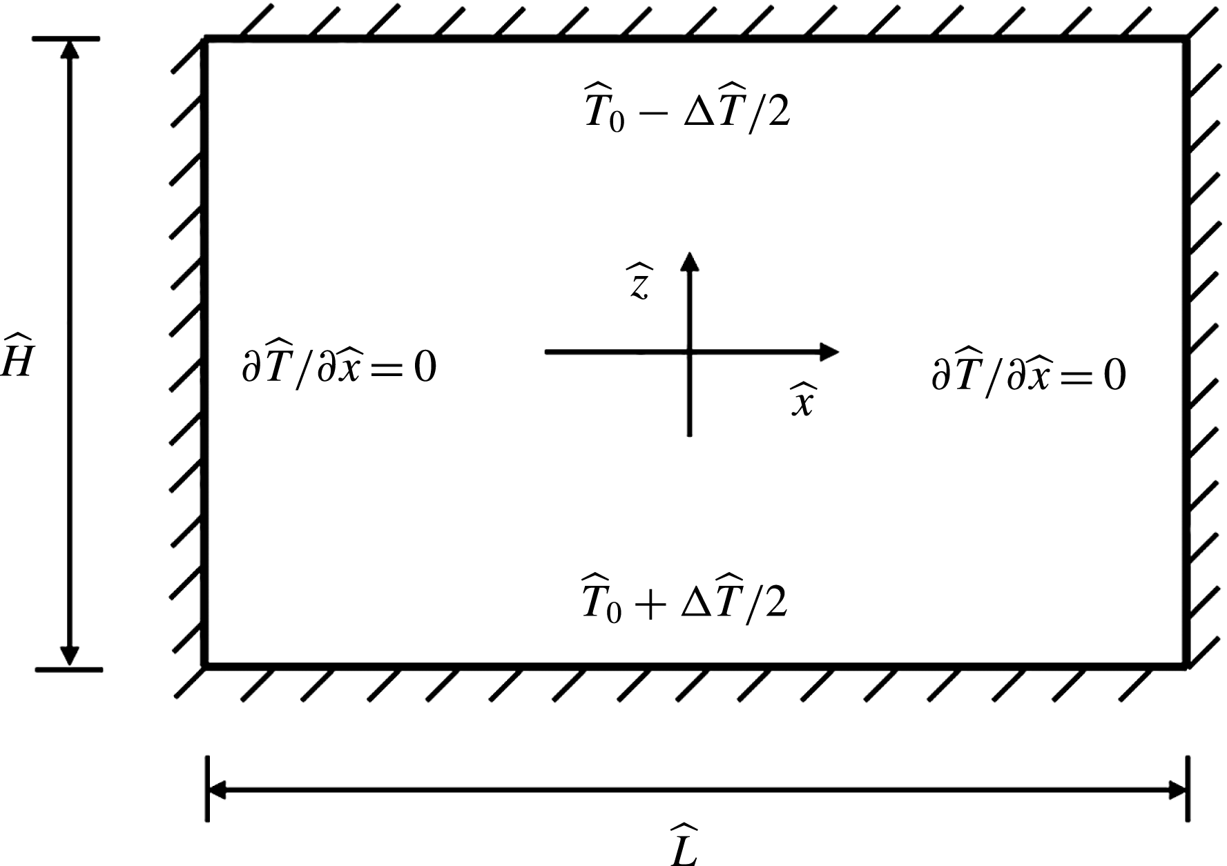
Schematic of two-dimensional RB system.

2 Problem description
The schematic of the two-dimensional RB system is illustrated in figure 1. The flow region is confined in a rigid cavity of height
 ${\hat{H}}$
and width
 $\hat{L}$
(hatted quantities are dimensional). The top and bottom plates are kept at constant temperatures, which are
 $\hat{T}_{0}-\unicode[STIX]{x0394}\hat{T}/2$
and
 $\hat{T}_{0}+\unicode[STIX]{x0394}\hat{T}/2$
, respectively, where
 $\unicode[STIX]{x0394}\hat{T}$
is the temperature drop across the fluid layer. The sidewalls are thermally insulated. In this paper air is used as the working fluid and the low-Mach-number equations with acoustic waves filtered are employed to describe the fluid flow (Paolucci Reference Paolucci1982). In dimensionless form the governing equations read
 $$\begin{eqnarray}\displaystyle \frac{\unicode[STIX]{x2202}\unicode[STIX]{x1D70C}}{\unicode[STIX]{x2202}t}+\frac{\unicode[STIX]{x2202}\unicode[STIX]{x1D70C}u_{j}}{\unicode[STIX]{x2202}x_{j}} & = & \displaystyle 0,\end{eqnarray}$$
 $$\begin{eqnarray}\displaystyle \frac{\unicode[STIX]{x2202}\unicode[STIX]{x1D70C}u_{i}}{\unicode[STIX]{x2202}t}+\frac{\unicode[STIX]{x2202}\unicode[STIX]{x1D70C}u_{i}u_{j}}{\unicode[STIX]{x2202}x_{j}}+\frac{\unicode[STIX]{x2202}\unicode[STIX]{x1D70B}}{\unicode[STIX]{x2202}x_{i}} & = & \displaystyle \sqrt{\frac{Pr}{Ra}}\frac{\unicode[STIX]{x2202}\unicode[STIX]{x1D70F}_{ij}}{\unicode[STIX]{x2202}x_{j}}+\frac{1}{2\unicode[STIX]{x1D716}}(\unicode[STIX]{x1D70C}-1)n_{i},\end{eqnarray}$$
 $$\begin{eqnarray}\displaystyle \unicode[STIX]{x1D70C}c_{p}\left(\frac{\unicode[STIX]{x2202}T}{\unicode[STIX]{x2202}t}+u_{j}\frac{\unicode[STIX]{x2202}T}{\unicode[STIX]{x2202}x_{j}}\right) & = & \displaystyle \frac{1}{\sqrt{RaPr}}\frac{\unicode[STIX]{x2202}}{\unicode[STIX]{x2202}x_{j}}\left(k\frac{\unicode[STIX]{x2202}T}{\unicode[STIX]{x2202}x_{j}}\right)+\unicode[STIX]{x1D6E4}\frac{\text{d}p}{\text{d}t},\end{eqnarray}$$
 $$\begin{eqnarray}\displaystyle p & = & \displaystyle \unicode[STIX]{x1D70C}T.\end{eqnarray}$$
Here
 $u_{i}=(u,w)$
denotes the velocity components along the horizontal and vertical directions
 $x_{i}=(x,z)$
;
 $T$
is the temperature and
 $\unicode[STIX]{x1D70C}$
the fluid density;
 $\unicode[STIX]{x1D70B}$
denotes the hydrodynamic pressure;
 $p$
represents the thermodynamic pressure, which is spatially constant;
 $\unicode[STIX]{x1D70F}_{ij}=\unicode[STIX]{x1D707}(\unicode[STIX]{x2202}u_{i}/\unicode[STIX]{x2202}x_{j}+\unicode[STIX]{x2202}u_{j}/\unicode[STIX]{x2202}x_{i})+\unicode[STIX]{x1D706}\unicode[STIX]{x1D6FF}_{ij}\unicode[STIX]{x2202}u_{k}/\unicode[STIX]{x2202}x_{k}$
is the viscosity stress tensor, where
 $\unicode[STIX]{x1D707}$
is the dynamical viscosity,
 $\unicode[STIX]{x1D706}=-2\unicode[STIX]{x1D707}/3$
is the volume viscosity and
 $\unicode[STIX]{x1D6FF}_{ij}$
is the Kronecker delta;
 $n_{i}=(0,-1)$
indicates the direction of gravity;
 $c_{p}$
is the isobaric specific heat, which is fixed at 1; and
 $\unicode[STIX]{x1D6E4}=(\unicode[STIX]{x1D6FE}-1)/\unicode[STIX]{x1D6FE}$
quantifies the resilience of the fluid, with the ratio of specific heats
 $\unicode[STIX]{x1D6FE}=1.4$
. Fluid viscosity
 $\unicode[STIX]{x1D707}$
and thermal conductivity
 $k$
are temperature-dependent and given by Sutherland’s law
 $$\begin{eqnarray}\displaystyle \unicode[STIX]{x1D707}=T^{3/2}\frac{1+S_{\unicode[STIX]{x1D707}}}{T+S_{\unicode[STIX]{x1D707}}},\quad k=T^{3/2}\frac{1+S_{k}}{T+S_{k}}, & & \displaystyle\end{eqnarray}$$
where
 $S_{\unicode[STIX]{x1D707}}=0.368$
and
 $S_{k}=0.648$
with reference temperature
 $\hat{T}_{0}=300~\text{K}$
. The arithmetic average temperature
 $\hat{T}_{0}$
, cavity height
 ${\hat{H}}$
, free-fall velocity
 $\hat{U} =(2\unicode[STIX]{x1D716}{\hat{g}}{\hat{H}})^{1/2}$
, reference time
 ${\hat{H}}/\hat{U}$
, average density
 $\hat{\unicode[STIX]{x1D70C}}_{0}$
, reference hydrodynamic pressure
 $\hat{\unicode[STIX]{x1D70C}}_{0}\hat{U} ^{2}$
and reference thermodynamic pressure
 $\hat{\unicode[STIX]{x1D70C}}_{0}\hat{R}\hat{T}_{0}$
are used to non-dimensionalize the equations, where
 ${\hat{g}}$
is the gravitational acceleration,
 $\hat{R}$
is the gas constant and
 $\unicode[STIX]{x1D716}$
is the dimensionless temperature differential, which will be defined later. Fluid properties evaluated at the reference temperature and thermodynamic pressure are also introduced as reference quantities, including
 ${\hat{c}}_{p0}$
,
 $\hat{\unicode[STIX]{x1D707}}_{0}$
and
 $\hat{k}_{0}$
.
The three dimensionless parameters in the governing equations are the Rayleigh number
 $Ra$
, the Prandtl number
 $Pr$
and the dimensionless temperature differential
 $\unicode[STIX]{x1D716}$
, which are defined as
 $$\begin{eqnarray}\displaystyle Ra=\frac{\unicode[STIX]{x0394}\hat{T}{\hat{c}}_{p0}\hat{\unicode[STIX]{x1D70C}}_{0}^{2}{\hat{g}}{\hat{H}}^{3}}{\hat{T}_{0}\hat{\unicode[STIX]{x1D707}}_{0}\hat{k}_{0}},\quad Pr=\frac{{\hat{c}}_{p0}\hat{\unicode[STIX]{x1D707}}_{0}}{\hat{k}_{0}},\quad \unicode[STIX]{x1D716}=\frac{\unicode[STIX]{x0394}\hat{T}}{2\hat{T}_{0}}. & & \displaystyle\end{eqnarray}$$
Besides these, there is a geometric parameter, i.e. the aspect ratio
 $A=\hat{L}/{\hat{H}}$
; the local Prandtl number is not spatially constant and varies slightly with temperature around the reference value 0.71 (Xia et al.
Reference Xia, Wan, Liu, Wang and Sun2016); and
 $\unicode[STIX]{x1D716}$
quantifies the intensity of NOB effects, with
 $\unicode[STIX]{x1D716}\leqslant 0.6$
corresponding to
 $\unicode[STIX]{x0394}\hat{T}\leqslant 360~\text{K}$
.
The governing equations are supplemented by the following boundary conditions:
 $$\begin{eqnarray}\displaystyle \left.\begin{array}{@{}c@{}}\displaystyle u=w=\frac{\unicode[STIX]{x2202}T}{\unicode[STIX]{x2202}x}=0,\quad \text{at}~x=\pm A/2,\\ \displaystyle u=w=0,\quad T=1\mp \unicode[STIX]{x1D716},\quad \text{at}~z=\pm 1/2.\end{array}\right\} & & \displaystyle\end{eqnarray}$$
Based on (2.1), (2.3) and (2.4) and the fact that the thermodynamic pressure
 $p$
is spatially constant, the time derivative of
 $p$
and velocity divergence can be obtained as
 $$\begin{eqnarray}\displaystyle \frac{\text{d}p}{\text{d}t} & = & \displaystyle \frac{1}{(1-\unicode[STIX]{x1D6E4})V}\frac{1}{\sqrt{RaPr}}\int _{V}\frac{\unicode[STIX]{x2202}}{\unicode[STIX]{x2202}x_{j}}\left(k\frac{\unicode[STIX]{x2202}T}{\unicode[STIX]{x2202}x_{j}}\right)\text{d}V,\end{eqnarray}$$
 $$\begin{eqnarray}\displaystyle \frac{\unicode[STIX]{x2202}u_{j}}{\unicode[STIX]{x2202}x_{j}} & = & \displaystyle \frac{1}{p}\left[(\unicode[STIX]{x1D6E4}-1)\frac{\text{d}p}{\text{d}t}+\frac{1}{\sqrt{RaPr}}\frac{\unicode[STIX]{x2202}}{\unicode[STIX]{x2202}x_{j}}\left(k\frac{\unicode[STIX]{x2202}T}{\unicode[STIX]{x2202}x_{j}}\right)\right]\nonumber\\ \displaystyle & = & \displaystyle \frac{1}{T}\left[\frac{\unicode[STIX]{x2202}T}{\unicode[STIX]{x2202}t}+u_{j}\frac{\unicode[STIX]{x2202}T}{\unicode[STIX]{x2202}x_{j}}-\frac{1}{\unicode[STIX]{x1D70C}}\frac{\text{d}p}{\text{d}t}\right],\end{eqnarray}$$
where
 $V$
is the cavity volume. Based on the equation of state (2.4) and global mass conservation condition,
 $p$
can be obtained as
 $$\begin{eqnarray}\displaystyle p=V\left(\int _{V}\frac{\text{d}V}{T}\right)^{-1}. & & \displaystyle\end{eqnarray}$$
In the limit
 $\unicode[STIX]{x1D716}\rightarrow 0$
, the OB approximation can be recovered from the low-Mach-number equations (Paolucci Reference Paolucci1982). In this study, quantities (e.g. the critical Rayleigh number for convection onset) within the OB approximation are estimated using the low-Mach-number equations with
 $\unicode[STIX]{x1D716}=10^{-5}$
, unless otherwise stated. Under the OB approximation, the RB system is equivariant under spatial reflections
 $R_{z}$
and
 $R_{x}$
about the horizontal and vertical mid-planes. The actions of these spatial transformations on the velocity field are given by
 $$\begin{eqnarray}\displaystyle \left.\begin{array}{@{}c@{}}\displaystyle R_{z}[u,w](t,x,z)=[u,-w](t,x,-z),\\ \displaystyle R_{x}[u,w](t,x,z)=[-u,w](t,-x,z).\end{array}\right\} & & \displaystyle\end{eqnarray}$$
When NOB effects are considered, the
 $R_{z}$
symmetry is broken and the system is equivariant only under spatial transformation
 $R_{x}$
. These symmetries play an important role in the bifurcation processes of the system (Golubitsky, Stewart & Schaeffer Reference Golubitsky, Stewart and Schaeffer1988; Crawford & Knobloch Reference Crawford and Knobloch1991; Hoyle Reference Hoyle2006).
Besides stability analysis, DNS is also performed. The governing equations are solved by a finite difference method with a second-order fractional-step method for time stepping and a second-order central difference scheme for spatial derivative terms. A non-uniform staggered grid is used with grid points clustered near walls. Our code was carefully validated and the DNS results are in good agreement with previous results in the literature. For more details see Xia et al. (Reference Xia, Wan, Liu, Wang and Sun2016).
3 Linear stability analysis
3.1 The base flow: thermal conduction state
The motionless conduction state is always a solution of the system and is stable when
 $Ra$
is small enough. Once the top and bottom boundary conditions are given, the distribution of temperature
 $\overline{T}$
(overline indicates quantities of the conduction state) can be determined by numerically solving the nonlinear equation (Chenoweth & Paolucci Reference Chenoweth and Paolucci1985)
 $$\begin{eqnarray}\displaystyle \frac{\text{d}}{\text{d}z}\left(\overline{k}\frac{\text{d}\overline{T}}{\text{d}z}\right)=0. & & \displaystyle\end{eqnarray}$$
Then other quantities of the conduction state (e.g.
 $\overline{p}$
,
 $\overline{\unicode[STIX]{x1D70C}}$
and
 $\overline{\unicode[STIX]{x1D70B}}$
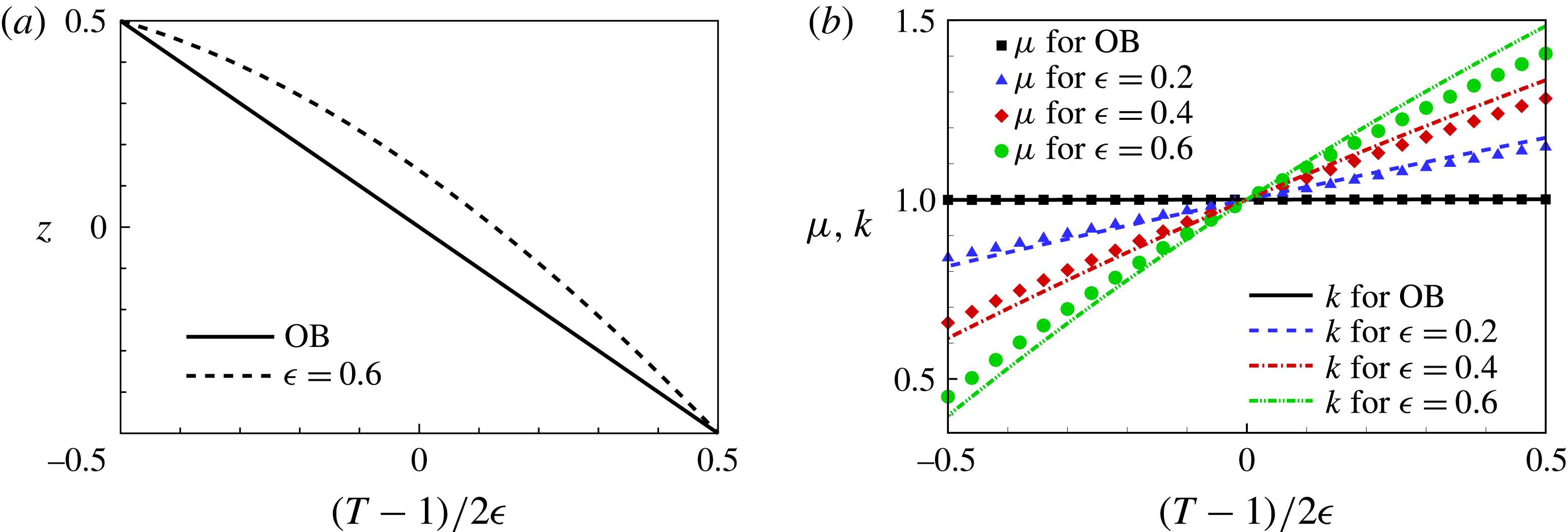
) can be obtained. Figure 2 shows the temperature profiles of the conduction states for the OB approximation and
 $\unicode[STIX]{x1D716}=0.6$
. The variations of
 $\unicode[STIX]{x1D707}$
and
 $k$
with
 $T$
are also shown. Within the OB approximation, the temperature varies linearly with
 $z$
. However, when
 $\unicode[STIX]{x1D716}=0.6$
, the linear relationship is lost and the temperature gradient is larger (smaller) near the cold (hot) horizontal plate. This is attributed to the fact that fluid conductivity
 $k$
is a monotonically increasing function of temperature as shown in figure 2(b).
(a) Temperature profiles of the conduction states for the OB approximation and NOB case
 $\unicode[STIX]{x1D716}=0.6$
. (b) Variations of
 $\unicode[STIX]{x1D707}$
and
 $k$
with
 $T$
.

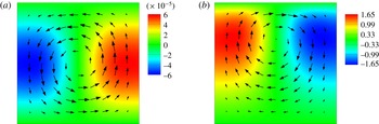
Disturbance velocity (arrows) and temperature (colour maps) distributions of critical eigenmodes for
 $A=1$
. (a) OB approximation, (b) NOB,
 $\unicode[STIX]{x1D716}=0.6$
.

3.2 Linear stability analysis and critical quantities
According to linear stability theory, the vector of dependent variables
 $\boldsymbol{q}=[u,w,T,\unicode[STIX]{x1D70B}]^{\text{T}}$
can be decomposed into two parts: the base flow
 $\overline{\boldsymbol{q}}$
and disturbance
 $\boldsymbol{q}^{\prime }$
. Substituting this decomposition into the fully nonlinear equations (2.2), (2.3) and (2.9), and neglecting the nonlinear terms of
 $\boldsymbol{q}^{\prime }$
, the following LSE is obtained, which governs the evolution of infinitesimal disturbance:
 $$\begin{eqnarray}\displaystyle \boldsymbol{C}\frac{\unicode[STIX]{x2202}\boldsymbol{q}^{\prime }}{\unicode[STIX]{x2202}t}=\boldsymbol{L}\boldsymbol{q}^{\prime }. & & \displaystyle\end{eqnarray}$$
Linear operators
 $\boldsymbol{C}$
and
 $\boldsymbol{L}$
are given in appendix A. Considering a normal-mode solution
 $$\begin{eqnarray}\displaystyle \boldsymbol{q}^{\prime }(t,x,z)=\tilde{\boldsymbol{q}}(x,z)\text{e}^{\unicode[STIX]{x1D70E}t}, & & \displaystyle\end{eqnarray}$$
and substituting it into (3.2), we obtain the boundary value equation
 $$\begin{eqnarray}\displaystyle \unicode[STIX]{x1D70E}\boldsymbol{C}\tilde{\boldsymbol{q}}=\boldsymbol{L}\tilde{\boldsymbol{q}}, & & \displaystyle\end{eqnarray}$$
which is supplemented with the homogeneous boundary conditions
 $$\begin{eqnarray}\displaystyle \left.\begin{array}{@{}c@{}}\displaystyle \tilde{u} =\tilde{w}=\frac{\unicode[STIX]{x2202}\tilde{T}}{\unicode[STIX]{x2202}x}=0,\quad \text{at }x=\pm A/2,\\ \displaystyle \tilde{u} =\tilde{w}=\tilde{T}=0,\quad \text{at}~z=\pm 1/2.\end{array}\right\} & & \displaystyle\end{eqnarray}$$
Here
 $\unicode[STIX]{x1D70E}$
denotes the growth rate of eigenmode
 $\tilde{\boldsymbol{q}}$
. The Chebyshev collocation method is used to discretize the boundary value equation above and the resulting matrix eigenvalue problem is solved using the QZ algorithm (Trefethen Reference Trefethen2000). Grid independence is verified for linear stability analysis and the leading eigenvalue is computed with an accuracy of at least
 $10^{-7}$
. For
 $A=1$
and
 $\unicode[STIX]{x1D716}=10^{-5}$
we obtain the critical Rayleigh number
 $Ra_{cr}$
of convection onset to be 2585.0187, which is in good agreement with the value 2585.0195 obtained by Mizushima (Reference Mizushima1995) based on the OB equations. When NOB effects are strong, the computed leading disturbance growth rate near criticality is also consistent with that obtained by DNS. Note that the instability of convection onset is found to be always stationary.
When
 $A=1$
, the critical eigenmodes for the OB approximation (
 $\unicode[STIX]{x1D716}=10^{-5}$
) and NOB case (
 $\unicode[STIX]{x1D716}=0.6$
) are depicted in figure 3. Compared with the OB case, it is clearly found that, under NOB conditions, the stagnation point of the dominant roll deviates from the mid-plane
 $z=0$
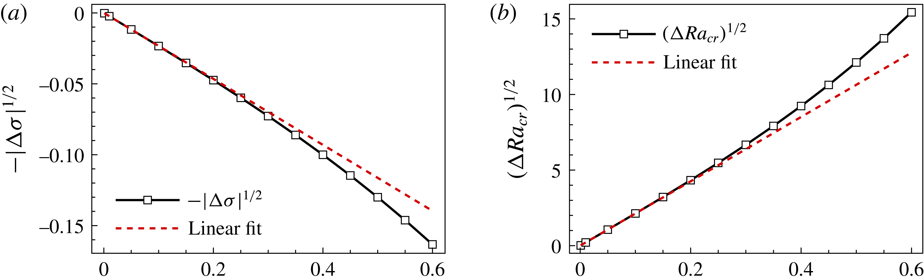
towards the cold plate, and the disturbance velocity and temperature gradient near the cold plate are larger than those near the hot plate. Variations of
 $-|\unicode[STIX]{x0394}\unicode[STIX]{x1D70E}|^{1/2}$
(for
 $Ra=2585.0187$
) and
 $(\unicode[STIX]{x0394}Ra_{cr})^{1/2}$
with
 $\unicode[STIX]{x1D716}$
are shown in figure 4, where
 $\unicode[STIX]{x0394}\unicode[STIX]{x1D70E}=\unicode[STIX]{x1D70E}(\unicode[STIX]{x1D716})-\unicode[STIX]{x1D70E}_{OB}$
and
 $\unicode[STIX]{x0394}Ra_{cr}=Ra_{cr}(\unicode[STIX]{x1D716})-Ra_{cr,OB}$
(subscript OB indicates quantities under the OB approximation). It is observed that both
 $-|\unicode[STIX]{x0394}\unicode[STIX]{x1D70E}|^{1/2}$
and
 $(\unicode[STIX]{x0394}Ra_{cr})^{1/2}$
are proportional to
 $\unicode[STIX]{x1D716}$
when
 $\unicode[STIX]{x1D716}$
is small. In other words,
 $\unicode[STIX]{x1D70E}$
and
 $Ra_{cr}$
vary with
 $\unicode[STIX]{x1D716}$
, with leading-order corrections
 ${\sim}\unicode[STIX]{x1D716}^{2}$
. For large
 $\unicode[STIX]{x1D716}$
, deviations from this
 $\unicode[STIX]{x1D716}^{2}$
scaling are visible. Based on numerical simulation of the low-Mach-number equations in a cavity of aspect ratio 20, Paolucci & Chenoweth (Reference Paolucci and Chenoweth1987) also observed the
 $\unicode[STIX]{x1D716}^{2}$
scaling of
 $\unicode[STIX]{x0394}Ra_{cr}$
and obtained the
 $Ra_{cr}$
–
 $\unicode[STIX]{x1D716}$
relation quantitatively.
Variations of (a)
 $-|\unicode[STIX]{x0394}\unicode[STIX]{x1D70E}|^{1/2}$
(for
 $Ra=2585.0187$
) and of (b)
 $(\unicode[STIX]{x0394}Ra_{cr})^{1/2}$
with
 $\unicode[STIX]{x1D716}$
for
 $A=1$
. Linear fits of small-
 $\unicode[STIX]{x1D716}$
data (red dashed lines) are also depicted, indicating that
 $-|\unicode[STIX]{x0394}\unicode[STIX]{x1D70E}|^{1/2}$
and
 $(\unicode[STIX]{x0394}Ra_{cr})^{1/2}$
are proportional to
 $\unicode[STIX]{x1D716}$
when
 $\unicode[STIX]{x1D716}$
is small.

This
 $\unicode[STIX]{x1D716}^{2}$
scaling originates from an intrinsic symmetry of the system. When
 $\unicode[STIX]{x1D716}$
changes sign and
 $Ra$
remains positive, the temperature boundary conditions of two horizontal plates are interchanged and the direction of gravity is reversed (due to the presence of
 $\unicode[STIX]{x1D716}$
in the buoyancy term). The resulting convection system is actually the same. Thus, the eigenvalues of the linear stability analysis are irrelevant to the sign of
 $\unicode[STIX]{x1D716}$
and
 $\tilde{\boldsymbol{q}}(-\unicode[STIX]{x1D716})=R_{z}[\tilde{\boldsymbol{q}}(+\unicode[STIX]{x1D716})]$
. We assume that the NOB influences on
 $\unicode[STIX]{x1D70E}$
and
 $Ra_{cr}$
can be accounted for by the following expansions in powers of
 $\unicode[STIX]{x1D716}$
:
 $$\begin{eqnarray}\displaystyle \left.\begin{array}{@{}c@{}}\unicode[STIX]{x1D70E}(\unicode[STIX]{x1D716})=\unicode[STIX]{x1D70E}_{OB}+\unicode[STIX]{x1D716}\unicode[STIX]{x1D70E}_{1}+\unicode[STIX]{x1D716}^{2}\unicode[STIX]{x1D70E}_{2}+\cdots \,,\\ Ra_{cr}(\unicode[STIX]{x1D716})=Ra_{cr,OB}+\unicode[STIX]{x1D716}R_{1}+\unicode[STIX]{x1D716}^{2}R_{2}+\cdots \,.\end{array}\right\} & & \displaystyle\end{eqnarray}$$
Then the intrinsic
 $\pm \unicode[STIX]{x1D716}$
symmetry implies
 $\unicode[STIX]{x1D70E}_{2n+1}=R_{2n+1}=0$
for
 $n=0,1,2,\ldots ,$
and the leading-order corrections of
 $\unicode[STIX]{x1D70E}$
and
 $Ra_{cr}$
due to NOB effects are at the order of
 $\unicode[STIX]{x1D716}^{2}$
.
3.3 Perturbation expansion of the LSE and influence of the aspect ratio
In order to quantitatively investigate flow instabilities of the conduction state with weak NOB effects, a perturbation expansion of the LSE in
 $\unicode[STIX]{x1D716}$
is performed. An analogous treatment of the LSE has been used in a variety of flow problems (Gao & Lu Reference Gao and Lu2006; Wang Reference Wang2008). Since instability of convection onset is found to be always stationary by linear stability analysis, it is appropriate to set the growth rate
 $\unicode[STIX]{x1D70E}$
to 0 in (3.4). Then
 $Ra_{cr}$
can be obtained by calculating the new eigenvalue
 $\unicode[STIX]{x1D706}=\sqrt{Ra_{cr}/Pr}$
of the resulting LSE.
Here we only consider the non-degenerate case, where only one eigenmode loses stability at criticality. Assume that the influences of weak NOB effects on
 $\unicode[STIX]{x1D706}$
can be accounted for by the following expansion in powers of
 $\unicode[STIX]{x1D716}$
:
 $$\begin{eqnarray}\displaystyle \unicode[STIX]{x1D706}=\unicode[STIX]{x1D706}_{0}+\unicode[STIX]{x1D716}\unicode[STIX]{x1D706}_{1}+\unicode[STIX]{x1D716}^{2}\unicode[STIX]{x1D706}_{2}+\cdots \,. & & \displaystyle\end{eqnarray}$$
Base flow
 $\overline{\boldsymbol{q}}=[\overline{u},\overline{w},\overline{T},\overline{\unicode[STIX]{x1D70B}}]^{\text{T}}$
and associated boundary conditions, linear operators of the LSE and eigenmode
 $\tilde{\boldsymbol{q}}=[\tilde{u} ,\tilde{w},\tilde{T},\tilde{\unicode[STIX]{x1D70B}}]^{\text{T}}$
are also expanded in
 $\unicode[STIX]{x1D716}$
analogously. Substituting these series expansions into the LSE and collecting terms of equal power of
 $\unicode[STIX]{x1D716}$
, a sequence of linear equations is obtained. The leading-order equation is of order
 $\unicode[STIX]{x1D716}^{-1}$
due to the presence of
 $\unicode[STIX]{x1D716}$
in the buoyancy term, and we obtain
 $\tilde{T}_{0}=0$
. At the order of
 $\unicode[STIX]{x1D716}^{0}$
, an eigenvalue problem is obtained:
 $$\begin{eqnarray}\displaystyle \unicode[STIX]{x1D706}_{0}\boldsymbol{B}\tilde{\boldsymbol{q}}_{0}=\boldsymbol{A}\tilde{\boldsymbol{q}}_{0}, & & \displaystyle\end{eqnarray}$$
where
 $\tilde{\boldsymbol{q}_{\mathbf{0}}}=[\tilde{u} _{0},\tilde{w}_{0},\tilde{T}_{1},\tilde{\unicode[STIX]{x1D70B}}_{0}]^{\text{T}}$
, and linear operators
 $\boldsymbol{A}$
and
 $\boldsymbol{B}$
are given in appendix B, and
 $\unicode[STIX]{x1D706}_{0}=\sqrt{Ra_{cr,OB}/Pr}$
and
 $\tilde{\boldsymbol{q}}_{0}$
are eigenpairs under the OB approximation. The smallest
 $\unicode[STIX]{x1D706}_{0}$
is of interest and gives the critical
 $Ra$
for convection onset. At the order of
 $\unicode[STIX]{x1D716}^{1}$
, we obtain an inhomogeneous equation
 $$\begin{eqnarray}\displaystyle \unicode[STIX]{x1D706}_{0}\boldsymbol{B}\tilde{\boldsymbol{q}}_{1}-\boldsymbol{A}\tilde{\boldsymbol{q}}_{1}=-(\unicode[STIX]{x1D706}_{1}\boldsymbol{B}\tilde{\boldsymbol{q}}_{0}+\boldsymbol{F}_{1}), & & \displaystyle\end{eqnarray}$$
where
 $\tilde{\boldsymbol{q}}_{1}=[\tilde{u} _{1},\tilde{w}_{1},\tilde{T}_{2},\tilde{\unicode[STIX]{x1D70B}}_{1}]^{\text{T}}$
and
 $\boldsymbol{F}_{1}$
is calculated from known quantities. Notice that the linear operator
 $\unicode[STIX]{x1D706}_{0}\boldsymbol{B}-\boldsymbol{A}$
is singular. In order to keep (3.9) solvable, the following orthogonality condition should be satisfied:
 $$\begin{eqnarray}\displaystyle \unicode[STIX]{x1D706}_{1}\tilde{\unicode[STIX]{x1D74D}}^{\text{H}}\boldsymbol{B}\tilde{\boldsymbol{q}}_{0}+\tilde{\unicode[STIX]{x1D74D}}^{\text{H}}\boldsymbol{F}_{1}=0, & & \displaystyle\end{eqnarray}$$
where
 $(\cdot )^{\text{H}}$
denotes complex-conjugate transpose and
 $\tilde{\unicode[STIX]{x1D74D}}$
is the critical adjoint eigenmode obtained by solving the adjoint eigenvalue problem
 $$\begin{eqnarray}\displaystyle \unicode[STIX]{x1D706}_{0}\boldsymbol{B}^{\text{H}}\tilde{\unicode[STIX]{x1D74D}}=\boldsymbol{A}^{\text{H}}\tilde{\unicode[STIX]{x1D74D}}. & & \displaystyle\end{eqnarray}$$
Normalization is performed so that
 $\tilde{\unicode[STIX]{x1D74D}}^{\text{H}}\boldsymbol{B}\tilde{\boldsymbol{q}}_{0}=1$
. When the compatibility condition (3.10) is satisfied,
 $\tilde{\boldsymbol{q}}_{1}$
is defined up to an arbitrary component of
 $\tilde{\boldsymbol{q}}_{0}$
. An additional condition
 $\tilde{\unicode[STIX]{x1D74D}}^{\text{H}}\boldsymbol{B}\tilde{\boldsymbol{q}}_{1}=0$
is introduced to uniquely determine
 $\tilde{\boldsymbol{q}}_{1}$
, which now quantifies the deviation of the eigenmode from that under the OB approximation. Then
 $\unicode[STIX]{x1D706}_{1}$
and
 $\tilde{\boldsymbol{q}}_{1}$
can be calculated at once by solving the bordered linear system (Carini, Auteri & Giannetti Reference Carini, Auteri and Giannetti2015)
 $$\begin{eqnarray}\displaystyle \left[\begin{array}{@{}cc@{}}\unicode[STIX]{x1D706}_{0}\boldsymbol{B}-\boldsymbol{A} & \boldsymbol{B}\tilde{\boldsymbol{q}}_{0}\\ \tilde{\unicode[STIX]{x1D74D}}^{\text{H}}\boldsymbol{B} & 0\end{array}\right]\left(\begin{array}{@{}c@{}}\tilde{\boldsymbol{q}}_{1}\\ \unicode[STIX]{x1D706}_{1}\end{array}\right)=\left(\begin{array}{@{}c@{}}-\boldsymbol{F}_{1}\\ 0\end{array}\right). & & \displaystyle\end{eqnarray}$$
At the order of
 $\unicode[STIX]{x1D716}^{2}$
, we obtain the equation
 $$\begin{eqnarray}\displaystyle \unicode[STIX]{x1D706}_{0}\boldsymbol{B}\tilde{\boldsymbol{q}}_{2}-\boldsymbol{A}\tilde{\boldsymbol{q}}_{2}=-(\unicode[STIX]{x1D706}_{2}\boldsymbol{B}\tilde{\boldsymbol{q}}_{0}+\boldsymbol{F}_{2}), & & \displaystyle\end{eqnarray}$$
where
 $\tilde{\boldsymbol{q}}_{2}=[\tilde{u} _{2},\tilde{w}_{2},\tilde{T}_{3},\tilde{\unicode[STIX]{x1D70B}}_{2}]^{\text{T}}$
and
 $\boldsymbol{F}_{2}$
is obtained from known quantities. The solvability condition of (3.13) yields
 $$\begin{eqnarray}\displaystyle \unicode[STIX]{x1D706}_{2}\tilde{\unicode[STIX]{x1D74D}}^{\text{H}}\boldsymbol{B}\tilde{\boldsymbol{q}}_{0}+\tilde{\unicode[STIX]{x1D74D}}^{\text{H}}\boldsymbol{F}_{2}=0. & & \displaystyle\end{eqnarray}$$
Then
 $\unicode[STIX]{x1D706}_{2}$
and
 $\tilde{\boldsymbol{q}}_{2}$
are also calculated at once by solving the bordered linear system
 $$\begin{eqnarray}\displaystyle \left[\begin{array}{@{}cc@{}}\unicode[STIX]{x1D706}_{0}\boldsymbol{B}-\boldsymbol{A} & \boldsymbol{B}\tilde{\boldsymbol{q}}_{0}\\ \tilde{\unicode[STIX]{x1D74D}}^{\text{H}}\boldsymbol{B} & 0\end{array}\right]\left(\begin{array}{@{}c@{}}\tilde{\boldsymbol{q}}_{2}\\ \unicode[STIX]{x1D706}_{2}\end{array}\right)=\left(\begin{array}{@{}c@{}}-\boldsymbol{F}_{2}\\ 0\end{array}\right). & & \displaystyle\end{eqnarray}$$
With homogeneous boundary conditions for
 $\tilde{\boldsymbol{q}}_{i}$
, the equations above are solved numerically using the Chebyshev collocation method for discretization, and the eigenvalue problem at the order of
 $\unicode[STIX]{x1D716}^{0}$
is solved using the QZ algorithm (Trefethen Reference Trefethen2000). The results show that generally
 $|\unicode[STIX]{x1D706}_{1}|\ll |\unicode[STIX]{x1D706}_{2}|$
and
 $|\unicode[STIX]{x1D706}_{1}|<10^{-6}$
for various
 $A$
, implying that
 $\unicode[STIX]{x0394}\unicode[STIX]{x1D706}=\unicode[STIX]{x1D706}(\unicode[STIX]{x1D716})-\unicode[STIX]{x1D706}_{0}$
is proportional to
 $\unicode[STIX]{x1D716}^{2}$
at the leading order. Since
 $\unicode[STIX]{x1D706}\sim \sqrt{Ra_{cr}}$
,
 $Ra_{cr}$
also varies with
 $\unicode[STIX]{x1D716}$
with a leading-order correction
 ${\sim}\unicode[STIX]{x1D716}^{2}$
, in qualitative consistency with the results of direct linear stability analysis and the
 $\pm \unicode[STIX]{x1D716}$
symmetry of the system. We attribute the small non-zero value of
 $\unicode[STIX]{x1D706}_{1}$
to numerical errors. The proportionality factor
 $2Pr\unicode[STIX]{x1D706}_{0}\unicode[STIX]{x1D706}_{2}$
between
 $\unicode[STIX]{x0394}Ra_{cr}$
and
 $\unicode[STIX]{x1D716}^{2}$
obtained by perturbation expansion of the LSE agrees well with that evaluated by direct linear stability analysis. The
 $\pm \unicode[STIX]{x1D716}$
symmetry implies that
 $\unicode[STIX]{x1D706}_{2n+1}$
be equal to 0 for
 $n=0,1,2,\ldots \,$
.
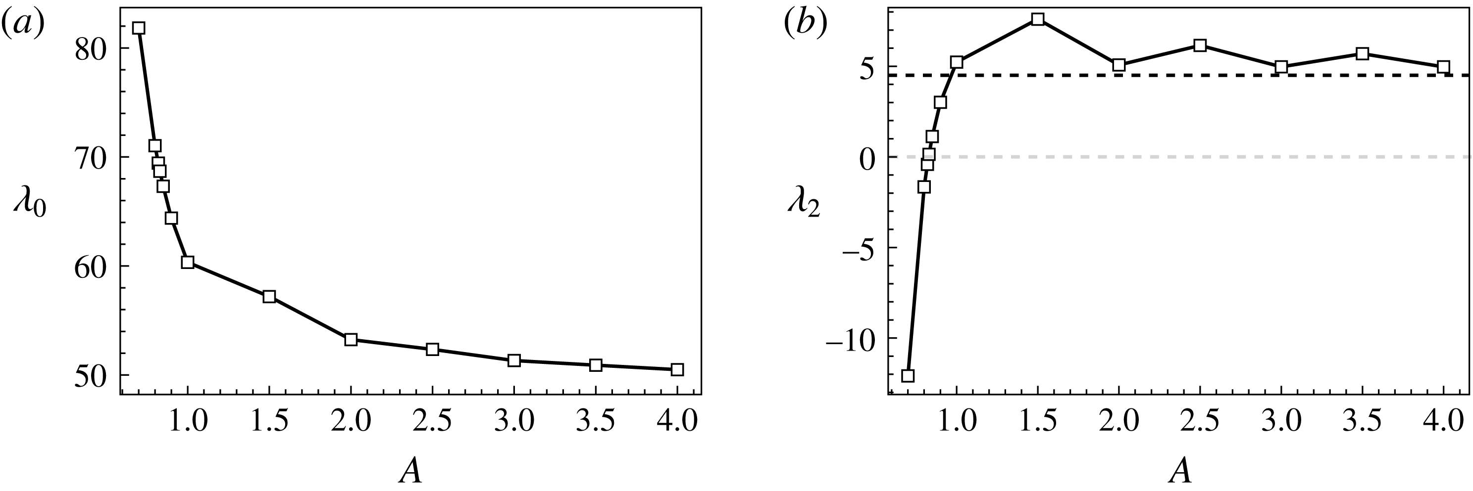
The variations of
 $\unicode[STIX]{x1D706}_{0}$
and
 $\unicode[STIX]{x1D706}_{2}$
with
 $A$
are shown in figure 5. From figure 5(a) it is observed that
 $\unicode[STIX]{x1D706}_{0}$
increases rapidly as
 $A\rightarrow 0$
and approaches
 $\sqrt{1708/Pr}$
asymptotically as
 $A\rightarrow \infty$
, which is in agreement with previous results (Mizushima Reference Mizushima1995). The value 1708 is the well-known critical Rayleigh number of an RB system of infinite extent under the OB approximation. From figure 5(b) it is found that the influences of weak NOB effects on stability of the conduction state are qualitatively different in wide and narrow cavities. When
 $A$
is large, we have
 $\unicode[STIX]{x1D706}_{2}>0$
, indicating that
 $Ra_{cr}$
increases with
 $\unicode[STIX]{x1D716}$
and flow stability is enhanced. When
 $A$
is small enough, we have
 $\unicode[STIX]{x1D706}_{2}<0$
, indicating that the conduction state is destabilized by NOB effects. The critical aspect ratio at which
 $\unicode[STIX]{x1D706}_{2}=0$
is approximately 0.83. By numerically solving the low-Mach-number equations, Paolucci & Chenoweth (Reference Paolucci and Chenoweth1987) found that
 $Ra_{cr}$
increases with
 $\unicode[STIX]{x1D716}$
as
 $Ra_{cr}=Ra_{c_{0}}(1+a\unicode[STIX]{x1D716}^{2})$
, with
 $Ra_{c_{0}}=1708.8$
and
 $a=0.1832$
in a cavity of aspect ratio 20. The corresponding
 $\unicode[STIX]{x1D706}_{2}$
can be evaluated as
 $a\sqrt{Ra_{c_{0}}}/2\sqrt{Pr}=4.49$
, which is consistent with the trend of
 $\unicode[STIX]{x1D706}_{2}$
in the wide-cavity limit obtained by perturbation expansion of the LSE, as shown in figure 5(b). We note that, while
 $\unicode[STIX]{x1D706}_{2}$
can be quantitatively dependent on the numerical values
 $S_{\unicode[STIX]{x1D707}}$
and
 $S_{k}$
for given
 $A$
, the trends of variation of
 $\unicode[STIX]{x1D706}_{2}$
with
 $A$
are qualitatively consistent for general perfect gases. Thus it is expected that the results obtained for air at reference temperature 300 K are generically valid for typical perfect gases.
Variations of (a)
 $\unicode[STIX]{x1D706}_{0}$
and (b)
 $\unicode[STIX]{x1D706}_{2}$
with
 $A$
. The black dashed line in (b) corresponds to the
 $\unicode[STIX]{x1D706}_{2}$
value computed based on numerical results of Paolucci & Chenoweth (Reference Paolucci and Chenoweth1987) for
 $A=20$
.

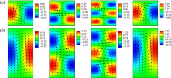
Distributions of temperature
 $\tilde{T}_{i+1}$
and velocity
 $(\tilde{u} _{i},\tilde{w}_{i})$
of
 $\tilde{\boldsymbol{q}}_{i}$
with
 $i=0,1,2$
for
 $A=1$
and 0.5 are depicted in figure 6. Eigenmodes
 $\tilde{\boldsymbol{q}}(\unicode[STIX]{x1D716}=0.1)$
obtained by perturbation expansion of the LSE are also shown. It is observed that, for both
 $A=1$
and 0.5,
 $\tilde{\boldsymbol{q}}_{0}$
comprises one dominant roll and
 $\tilde{\boldsymbol{q}}_{1}$
comprises two vertically stacked rolls. However, the velocity distributions of
 $\tilde{\boldsymbol{q}}_{2}$
are different for the two aspect ratios. For
 $A=0.5$
,
 $\tilde{\boldsymbol{q}}_{2}$
consists of three well-developed vertically stacked rolls, while for
 $A=1$
, only two rolls are present. This is attributed to the larger vertical extent in narrower cavities. As the cavity is widened, the strength and vertical dimension of the middle roll of the velocity field decrease gradually, while there is little change in the size of associated temperature blocks. Thus mismatch of the velocity and temperature fields appears in wide cavities, as shown in the third panel of figure 6(a). Despite the existence of mismatch, the temperature and velocity fields are always consistent with each other in terms of symmetries. For both aspect ratios
 $A=1$
and 0.5,
 $\tilde{\boldsymbol{q}}(\unicode[STIX]{x1D716}=0.1)$
consists of one dominant roll. The distinctions of NOB corrections of eigenmodes for the two aspect ratios are expected to lead to different disturbance kinetic energy budget variations as shown in the following section (§ 3.4) and result in qualitatively different NOB influences of linear instabilities. When
 $\tilde{\boldsymbol{q}}_{1}$
of appropriate amplitude is superposed on
 $\tilde{\boldsymbol{q}}_{0}$
, temperature gradient and velocity are enlarged (reduced) near the cold (hot) plate, and the stagnation point of the dominant roll deviates from the horizontal mid-plane towards the cold plate, consistent with previous observation (see figure 3).
Velocity (arrows) and temperature (colour maps) distributions of
 $\tilde{\boldsymbol{q}}_{0}$
,
 $\tilde{\boldsymbol{q}}_{1}$
,
 $\tilde{\boldsymbol{q}}_{2}$
and
 $\tilde{\boldsymbol{q}}(\unicode[STIX]{x1D716}=0.1)$
(from left to right) for (a)
 $A=1$
and (b)
 $A=0.5$
.

When
 $\unicode[STIX]{x1D716}=0.1$
, the critical Rayleigh numbers
 $Ra_{cr}$
calculated by perturbation expansion are 2589.5 and 11921 for
 $A=1$
and 0.5, respectively. The most unstable eigenmodes at these two parameter combinations
 $(Ra_{cr},A)$
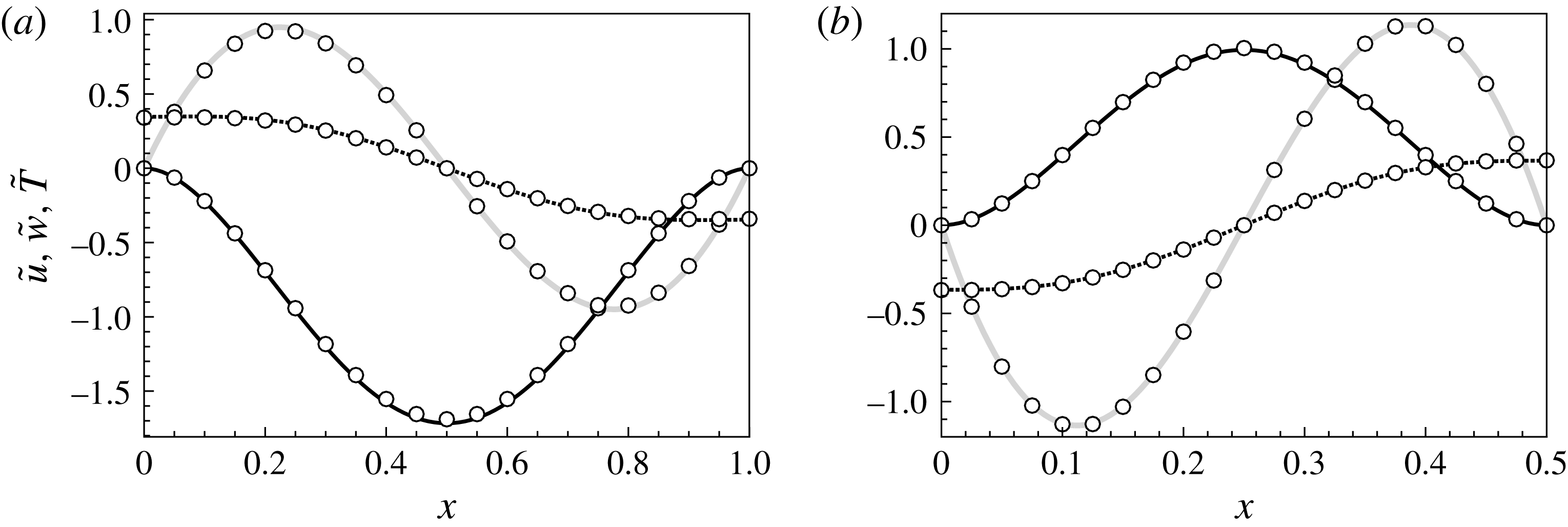
are obtained by direct linear stability analysis. Then the temperature and velocity profiles along the cross-section
 $z=0.25$
are extracted and compared with those obtained by perturbation expansion, as shown in figure 7. Good quantitative agreement is obtained.
Profiles of
 $\tilde{u}$
(black solid line),
 $\tilde{w}$
(grey solid line) and
 $\tilde{T}$
(black dashed line) along the cross-section
 $z=0.25$
of
 $\tilde{\boldsymbol{q}}(\unicode[STIX]{x1D716}=0.1)$
obtained by perturbation expansion for (a)
 $A=1$
and (b)
 $A=0.5$
. Results of direct linear stability analysis (circles) are also shown for comparison.

The distributions of
 $\tilde{\boldsymbol{q}}_{0}$
,
 $\tilde{\boldsymbol{q}}_{1}$
and
 $\tilde{\boldsymbol{q}}_{2}$
in figure 6 can be shown to be consistent with the
 $\pm \unicode[STIX]{x1D716}$
symmetry of the system. It is observed that
 $\{\tilde{u} _{i},\tilde{w}_{i},\tilde{T}_{i}\}$
can be classified into two sets based on symmetry. Quantities in set
 $S_{e}=\{\tilde{u} _{0},\tilde{u} _{2},\tilde{w}_{0},\tilde{w}_{2},\tilde{T}_{2}\}$
have even indices and are invariant under
 $R_{x}R_{z}$
transformation, while those in set
 $S_{o}=\{\tilde{u} _{1},\tilde{w}_{1},\tilde{T}_{1},\tilde{T}_{3}\}$
have odd indices and are invariant under
 $R_{z}$
transformation. We denote these symmetries as
 $R_{x}R_{z}[S_{e}]=S_{e}$
and
 $R_{z}[S_{o}]=S_{o}$
. Note that
 $R_{x}[S_{e}]=R_{z}[S_{e}]=-S_{e}$
and
 $R_{x}[S_{o}]=-S_{o}$
. By perturbation expansion eigenmode
 $\tilde{\boldsymbol{q}}(\unicode[STIX]{x1D716})$
can be obtained by linear combination of
 $S_{e}$
and
 $S_{o}$
, which is denoted as
 $\tilde{\boldsymbol{q}}(\unicode[STIX]{x1D716})=f([S_{e},S_{o}],\unicode[STIX]{x1D716})$
formally;
 $f$
has the properties
 $f([S_{e},S_{o}],-\unicode[STIX]{x1D716})=f([S_{e},-S_{o}],\unicode[STIX]{x1D716})$
and
 $R[f([S_{e},S_{o}],\unicode[STIX]{x1D716})]=f(R[S_{e},S_{o}],\unicode[STIX]{x1D716})$
for transformation
 $R\in \{R_{x},R_{z},R_{x}R_{z}\}$
. Then it can be shown that
 $$\begin{eqnarray}\displaystyle R_{z}[\tilde{\boldsymbol{q}}(\unicode[STIX]{x1D716})]=R_{z}[f([S_{e},S_{o}],\unicode[STIX]{x1D716})]=R_{x}[f([S_{e},S_{o}],-\unicode[STIX]{x1D716})]=R_{x}[\tilde{\boldsymbol{q}}(-\unicode[STIX]{x1D716})]. & & \displaystyle\end{eqnarray}$$
Here
 $\tilde{\boldsymbol{q}}(-\unicode[STIX]{x1D716})$
is the eigenmode for the RB system with dimensionless temperature differential
 $-\unicode[STIX]{x1D716}$
, so
 $R_{x}[\tilde{\boldsymbol{q}}(-\unicode[STIX]{x1D716})]$
is due to the
 $R_{x}$
reflection symmetry, which is consistent with the
 $\pm \unicode[STIX]{x1D716}$
symmetry of the system.
3.4 Energy analysis
In order to gain detailed physical insights into the NOB influences on flow instability, a budget analysis of disturbance kinetic energy near convection onset is performed, and the contributions of different physical factors to disturbance growth rate are quantitatively identified. The rate of change of disturbance kinetic energy is governed by the Reynolds–Orr equation, which is obtained by multiplying the linear momentum equation by
 $\boldsymbol{u}^{\prime }$
and integrating over the flow domain
 $V$
(Ma, Henry & Hadid Reference Ma, Henry and Hadid2005; Wang et al.
Reference Wang, Ma, Chen and Sun2012, Reference Wang, Wan, Guo, Ma and Sun2014):
 $$\begin{eqnarray}\displaystyle \frac{1}{K}\frac{\text{d}K}{\text{d}t}=\underbrace{-\frac{1}{K}\int _{V}{u^{\prime }}_{i}\frac{\unicode[STIX]{x2202}\unicode[STIX]{x1D70B}^{\prime }}{\unicode[STIX]{x2202}x_{i}}\,\text{d}V}_{k_{c}}+\underbrace{\frac{1}{K}\sqrt{\frac{Pr}{Ra}}\int _{V}{u^{\prime }}_{i}\frac{\unicode[STIX]{x2202}{\unicode[STIX]{x1D70F}^{\prime }}_{ij}}{\unicode[STIX]{x2202}x_{j}}\,\text{d}V}_{k_{v}}+\underbrace{\frac{1}{K}\frac{1}{2\unicode[STIX]{x1D716}}\int _{V}\unicode[STIX]{x1D70C}^{\prime }n_{i}{u^{\prime }}_{i}\,\text{d}V}_{k_{b}}, & & \displaystyle\end{eqnarray}$$
where
 $K=(1/2)\int _{V}\unicode[STIX]{x1D70C}_{0}u_{i}^{\prime }u_{i}^{\prime }\,\text{d}V$
is the disturbance kinetic energy, and terms
 $k_{c}$
,
 $k_{v}$
and
 $k_{b}$
correspond to the overall contributions of compressibility, viscosity and buoyancy, respectively.
For
 $i\in \{c,v,b\}$
, the variations of
 $k_{i}$
due to NOB effects are quantified by
 $\unicode[STIX]{x0394}k_{i}=k_{i}(\unicode[STIX]{x1D716})-k_{i,OB}$
. We use
 $k_{s}=|\unicode[STIX]{x0394}k_{c}|+|\unicode[STIX]{x0394}k_{v}|+|\unicode[STIX]{x0394}k_{b}|$
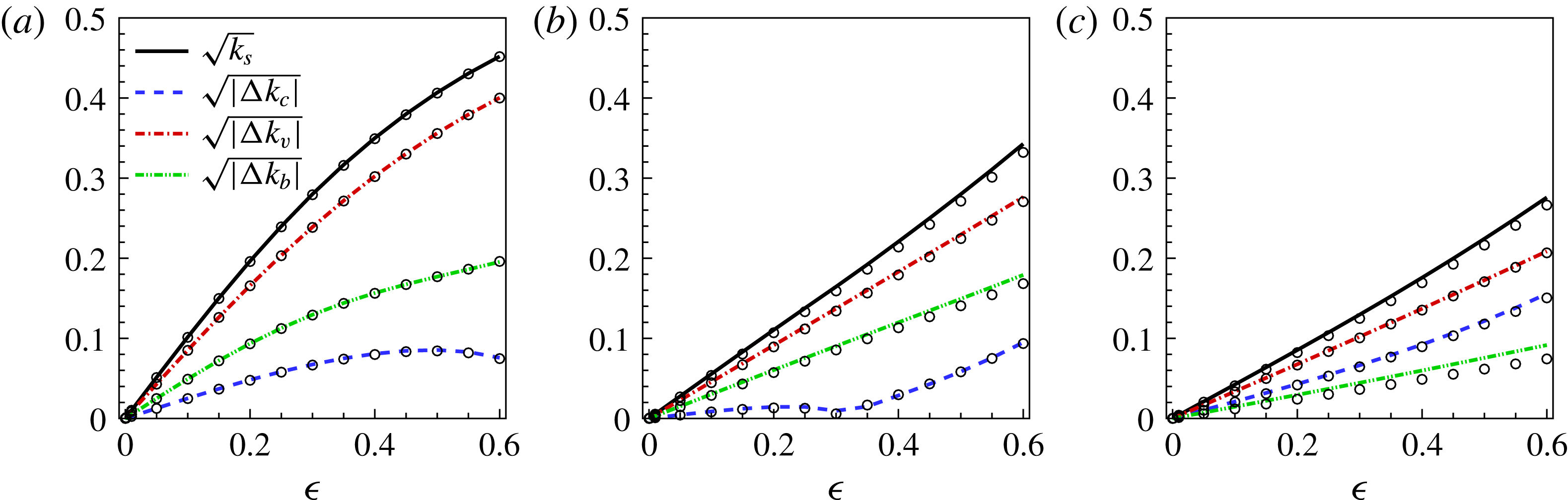
to measure the overall sensitivity of different actions to NOB effects. A budget analysis of disturbance kinetic energy near criticality is performed for
 $A=0.6,~1,~2.5$
, and the variations of
 $k_{s}$
and
 $\unicode[STIX]{x0394}k_{i}$
with
 $\unicode[STIX]{x1D716}$
are obtained, as depicted in figure 8. For each
 $A$
, results at two Rayleigh numbers with a difference of approximately 100 are shown. It is found that the variations of results at the two different Rayleigh numbers are fairly small, suggesting that
 $k_{s}$
and
 $\unicode[STIX]{x0394}k_{i}$
as functions of
 $\unicode[STIX]{x1D716}$
and
 $Ra$
depend weakly on
 $Ra$
near criticality. Therefore, in the following, the NOB influences on disturbance kinetic energy budget are investigated without explicit consideration of the influence of
 $Ra$
.
In figure 8, it is noteworthy that
 $\sqrt{k_{s}}$
and
 $\sqrt{|\unicode[STIX]{x0394}k_{i}|}$
vary with
 $\unicode[STIX]{x1D716}$
linearly when
 $\unicode[STIX]{x1D716}$
is small. In other words,
 $k_{s}$
and
 $\unicode[STIX]{x0394}k_{i}$
are proportional to
 $\unicode[STIX]{x1D716}^{2}$
for small
 $\unicode[STIX]{x1D716}$
, which can also be interpreted in terms of the
 $\pm \unicode[STIX]{x1D716}$
symmetry of the system. This scaling is approximately valid for a fairly large
 $\unicode[STIX]{x1D716}$
range, especially for
 $A=1$
and 2.5. The complex variation of
 $\sqrt{|\unicode[STIX]{x0394}k_{c}|}$
in the case
 $A=1$
is due to the fact that, as
 $\unicode[STIX]{x1D716}$
is increased,
 $k_{c}$
first increases from 0 and then decreases and becomes negative for large
 $\unicode[STIX]{x1D716}$
. This indicates that compressibility has both stabilizing and destabilizing effects, depending on the intensity of NOB effects. It is found that
 $k_{v}$
is always negative, indicating the stabilizing effect of viscosity, while
 $k_{b}$
is always positive, indicating the destabilizing effect of buoyancy. Since
 $k_{s}$
and
 $\unicode[STIX]{x0394}k_{i}$
comply with the same scaling with
 $\unicode[STIX]{x1D716}$
in a certain range of
 $\unicode[STIX]{x1D716}$
,
 $\unicode[STIX]{x0394}k_{i}/k_{s}$
are basically
 $\unicode[STIX]{x1D716}$
-independent.
Plots of
 $\sqrt{k_{s}}$
,
 $\sqrt{|\unicode[STIX]{x0394}k_{c}|}$
,
 $\sqrt{|\unicode[STIX]{x0394}k_{v}|}$
and
 $\sqrt{|\unicode[STIX]{x0394}k_{b}|}$
as functions of
 $\unicode[STIX]{x1D716}$
for different
 $(Ra,A)$
combinations: (a)
 $(Ra,A)=(6950,0.6)$
(lines) and
 $(Ra,A)=(7054,0.6)$
(circles); (b)
 $(Ra,A)=(2570,1)$
(lines) and
 $(Ra,A)=(2670,1)$
(circles); and (c)
 $(Ra,A)=(1900,2.5)$
(lines) and
 $(Ra,A)=(2000,2.5)$
(circles).

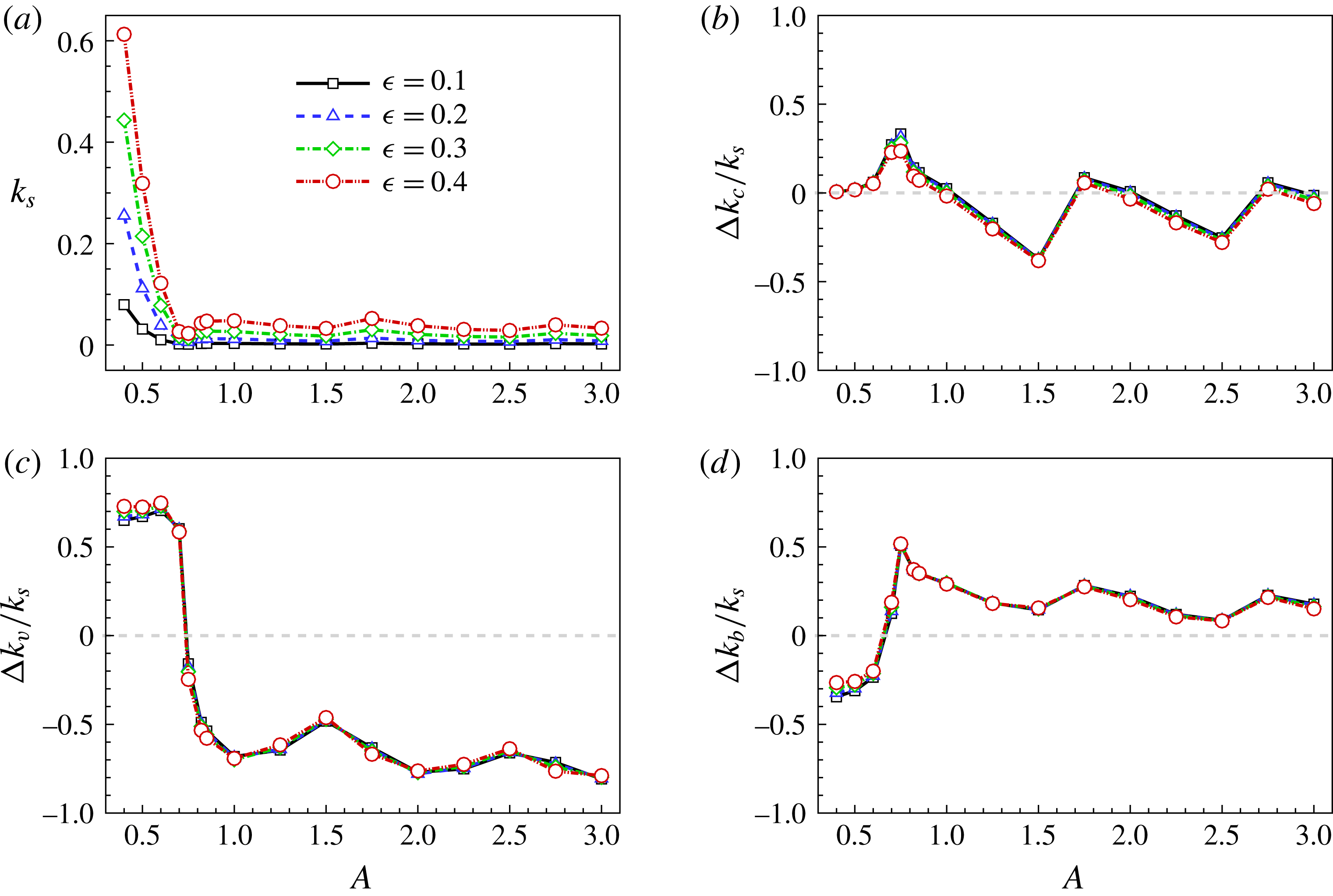
Figure 9 plots the variations of
 $k_{s}$
and
 $\unicode[STIX]{x0394}k_{i}/k_{s}$
with
 $A$
for
 $\unicode[STIX]{x1D716}=0.1$
, 0.2, 0.3 and 0.4. As we can see, the data of
 $\unicode[STIX]{x0394}k_{i}/k_{s}$
at various
 $\unicode[STIX]{x1D716}$
are collapsed fairly well onto the same curves. From figure 9(a) it is found that
 $k_{s}$
is basically independent on
 $A$
for large
 $A$
. However, when
 $A$
is small enough,
 $k_{s}$
grows rapidly as
 $A$
is decreased, indicating that the overall sensitivity of compressibility, viscosity and buoyancy actions to NOB effects is larger in narrow cavities. From figure 9(b) it is observed that
 $\unicode[STIX]{x0394}k_{c}$
can be positive or negative for different
 $A$
. Since
 $k_{c,OB}=0$
,
 $k_{c}$
can be positive or negative, implying that compressibility may weaken or enhance flow stability for various
 $A$
under NOB conditions. From figure 9(c,d), it is observed that
 $\unicode[STIX]{x0394}k_{v}$
(
 $\unicode[STIX]{x0394}k_{b}$
) is positive (negative) for small
 $A$
and becomes negative (positive) for large
 $A$
. Considering that
 $k_{v}<0$
and
 $k_{b}>0$
, the variations of
 $\unicode[STIX]{x0394}k_{v}$
and
 $\unicode[STIX]{x0394}k_{b}$
with
 $A$
indicate that viscosity and buoyancy actions are weakened (enhanced) for small (large)
 $A$
on account of NOB effects. From figure 9(b–d),
 $|\unicode[STIX]{x0394}k_{v}/k_{s}|$
is observed to be larger than
 $|\unicode[STIX]{x0394}k_{c}/k_{s}|$
and
 $|\unicode[STIX]{x0394}k_{b}/k_{s}|$
generally (except near the transition point from being positive to negative), implying that, compared with compressibility and buoyancy, viscosity action is more sensitive to NOB effects and the NOB influences on disturbance growth rate are dominated by the variation of
 $k_{v}$
.
Plots of (a)
 $k_{s}$
, (b)
 $\unicode[STIX]{x0394}k_{c}/k_{s}$
, (c)
 $\unicode[STIX]{x0394}k_{v}/k_{s}$
and (d)
 $\unicode[STIX]{x0394}k_{b}/k_{s}$
as functions of
 $A$
for
 $\unicode[STIX]{x1D716}=0.1$
, 0.2, 0.3 and 0.4.

We note that
 $k_{i}$
are the integral contributions of corresponding actions. We can further divide them into contributions originating from different components of
 $k_{i}$
and different locations of the flow domain. It is found that the NOB corrections can be stabilizing or destabilizing depending on the specific components and spatial locations, indicating that the NOB corrections
 $\unicode[STIX]{x0394}k_{i}$
originate from the competition of various components and spatial locations.
4 Weakly nonlinear analysis
4.1 Basic formulations of weakly nonlinear analysis
In order to investigate the NOB influences on bifurcation characteristics of convection onset, weakly nonlinear analysis is performed based on centre-manifold reduction. Necessary formulations are described in this subsection. A more complete and rigorous discussion can be found in Coullet & Spiegel (Reference Coullet and Spiegel1983) and Carini et al. (Reference Carini, Auteri and Giannetti2015). In this study,
 $Ra$
and
 $A$
constitute the parameter space and
 $\unicode[STIX]{x1D716}$
is treated as an external parameter. At certain parameter values (
 $Ra_{cr},A_{cr}$
), two eigenmodes can lose stability simultaneously. Near these so-called codimension-two points, two reduced control parameters are introduced:
 $$\begin{eqnarray}\displaystyle \unicode[STIX]{x1D709}=\frac{1}{\sqrt{Ra_{cr}}}-\frac{1}{\sqrt{Ra}},\quad \unicode[STIX]{x1D701}=\frac{1}{A}-\frac{1}{A_{cr}}. & & \displaystyle\end{eqnarray}$$
Here
 $A$
is a geometric parameter appearing in the boundary conditions (2.7). It is convenient to rescale the
 $x$
-coordinate so that parameter
 $A$
appears explicitly in the governing equations. Decomposing the vector of dependent variables
 $\boldsymbol{q}=[u,w,T,\unicode[STIX]{x1D70B}]^{\text{T}}$
into base flow
 $\overline{\boldsymbol{q}}$
and disturbance
 $\boldsymbol{q}^{\prime }$
, the following nonlinear disturbance equation is obtained from the fully nonlinear equations (2.2), (2.3) and (2.9):
 $$\begin{eqnarray}\displaystyle \boldsymbol{C}^{w}\frac{\unicode[STIX]{x2202}\boldsymbol{q}^{\prime }}{\unicode[STIX]{x2202}t}=\boldsymbol{L}^{w}\boldsymbol{q}^{\prime }+\boldsymbol{N}^{w}(\boldsymbol{q}^{\prime },\unicode[STIX]{x1D709},\unicode[STIX]{x1D701}), & & \displaystyle\end{eqnarray}$$
where linear operators
 $\boldsymbol{C}^{w}$
and
 $\boldsymbol{L}^{w}$
are the rescaled counterparts of
 $\boldsymbol{C}$
and
 $\boldsymbol{L}$
in (3.2) with parameters
 $(Ra,A)=(Ra_{cr},A_{cr})$
. Nonlinear terms of
 $\boldsymbol{q}^{\prime }$
are collected in
 $\boldsymbol{N}^{w}$
;
 $\boldsymbol{q}^{\prime }$
can be expressed as a function of critical amplitudes
 $\boldsymbol{a}=(\unicode[STIX]{x1D6FC},\unicode[STIX]{x1D6FD})$
of two critical eigenmodes and bifurcation parameters
 $\boldsymbol{b}=(\unicode[STIX]{x1D709},\unicode[STIX]{x1D701})$
(Carini et al.
Reference Carini, Auteri and Giannetti2015)
 $$\begin{eqnarray}\displaystyle \boldsymbol{q}^{\prime }(t)=\boldsymbol{q}^{\prime }(\boldsymbol{a}(t),\boldsymbol{b}). & & \displaystyle\end{eqnarray}$$
The dynamics of a system restricted on the centre manifold is governed by the reduced-order equation
 $$\begin{eqnarray}\displaystyle \dot{\boldsymbol{a}}=\boldsymbol{g}(\boldsymbol{a}(t),\boldsymbol{b}). & & \displaystyle\end{eqnarray}$$
Based on centre-manifold reduction, we can expand
 $\boldsymbol{q}^{\prime }(\boldsymbol{a}(t),\boldsymbol{b})$
and
 $\boldsymbol{g}(\boldsymbol{a}(t),\boldsymbol{b})$
as power series of
 $\boldsymbol{a}$
and
 $\boldsymbol{b}$
as
 $$\begin{eqnarray}\displaystyle \left.\begin{array}{@{}c@{}}\displaystyle \boldsymbol{q}^{\prime }(\boldsymbol{a}(t),\boldsymbol{b})=\mathop{\sum }_{m=1}^{\overline{r}}\mathop{\sum }_{|\boldsymbol{i}|+|\boldsymbol{j}|=m}\tilde{\boldsymbol{q}}_{\boldsymbol{i},\boldsymbol{j}}\boldsymbol{a}^{\boldsymbol{i}}(t)\boldsymbol{b}^{\boldsymbol{j}},\\ \displaystyle \boldsymbol{g}(\boldsymbol{a}(t),\boldsymbol{b})=\mathop{\sum }_{m=1}^{\overline{r}}\mathop{\sum }_{|\boldsymbol{i}|+|\boldsymbol{j}|=m}\tilde{\boldsymbol{g}}_{\boldsymbol{i},\boldsymbol{j}}\boldsymbol{a}^{\boldsymbol{i}}(t)\boldsymbol{b}^{\boldsymbol{j}},\end{array}\right\} & & \displaystyle\end{eqnarray}$$
where, following the notations in Carini et al. (Reference Carini, Auteri and Giannetti2015),
 $\boldsymbol{i}=(i_{1},i_{2})$
and
 $\boldsymbol{j}=(j_{1},j_{2})$
are multi-indices,
 $|\boldsymbol{i}|=i_{1}+i_{2}$
,
 $|\boldsymbol{j}|=j_{1}+j_{2}$
and
 $\boldsymbol{a}^{\boldsymbol{i}}\boldsymbol{b}^{\boldsymbol{j}}=\unicode[STIX]{x1D6FC}^{i_{1}}\unicode[STIX]{x1D6FD}^{i_{2}}\unicode[STIX]{x1D709}^{j_{1}}\unicode[STIX]{x1D701}^{j_{2}}$
; and
 $\overline{r}$
is the finite truncation order.
Substituting expressions (4.5) into the nonlinear disturbance equation (4.2), terms of the same order
 $(\boldsymbol{m},\boldsymbol{k})$
are collected, leading to a sequence of linear equations, the solutions of which give
 $\tilde{\boldsymbol{q}}_{\boldsymbol{i},\boldsymbol{j}}$
and
 $\tilde{\boldsymbol{g}}_{\boldsymbol{i},\boldsymbol{j}}$
. Thus, the low-dimensional amplitude equation (4.4) is constructed. For the generic term
 $(\boldsymbol{m},\boldsymbol{k})$
, we obtain
 $$\begin{eqnarray}\displaystyle \mathop{\left\langle \boldsymbol{C}^{w}\mathop{\sum }_{m=1}^{\overline{r}}\mathop{\sum }_{|\boldsymbol{i}|+|\boldsymbol{j}|=m}\tilde{\boldsymbol{q}}_{\boldsymbol{i},\boldsymbol{j}}(\dot{\boldsymbol{a}^{\boldsymbol{i}}})\boldsymbol{b}^{\boldsymbol{j}}\right\rangle }\nolimits_{\boldsymbol{m},\boldsymbol{k}}=\boldsymbol{L}^{w}\tilde{\boldsymbol{q}}_{\boldsymbol{m},\boldsymbol{k}}+\langle \boldsymbol{N}^{w}(\boldsymbol{q}^{\prime },\boldsymbol{b})\rangle _{\boldsymbol{m},\boldsymbol{k}}, & & \displaystyle\end{eqnarray}$$
where
 $\langle \boldsymbol{f}\rangle _{\boldsymbol{m},\boldsymbol{k}}$
indicates the vector coefficient of
 $\boldsymbol{a}^{\boldsymbol{m}}\boldsymbol{b}^{\boldsymbol{k}}$
in power series expansion of
 $\boldsymbol{f}$
. Note that approximate algebraic expressions for
 $\unicode[STIX]{x1D707}(T)$
and
 $k(T)$
are employed, which are derived by expanding Sutherland’s law (2.5a,b
) in Taylor series about
 $\overline{T}$
up to order
 $\overline{r}$
.
As in Carini et al. (Reference Carini, Auteri and Giannetti2015), a two-dimensional multi-index
 $\mathbf{1}_{l}$
is introduced for convenience whose
 $l$
th entry is one and the other is set to zero. Let us consider the order
 $\overline{m}=1$
first, where
 $\overline{m}=|\boldsymbol{m}|+|\boldsymbol{k}|$
. When
 $(\boldsymbol{m},\boldsymbol{k})=(\mathbf{1}_{l},\mathbf{0})$
for
 $l=1,2$
, assuming
 $\tilde{\boldsymbol{g}}_{\mathbf{1}_{l},\mathbf{0}}=\unicode[STIX]{x1D70E}_{l}\mathbf{1}_{l}$
(Carini et al.
Reference Carini, Auteri and Giannetti2015), the following generalized eigenvalue problem is obtained (
 $\boldsymbol{N}^{w}$
does not contribute at this order):
 $$\begin{eqnarray}\displaystyle \unicode[STIX]{x1D70E}_{l}\boldsymbol{C}^{w}\tilde{\boldsymbol{q}}_{\mathbf{1}_{l},\mathbf{0}}=\boldsymbol{L}^{w}\tilde{\boldsymbol{q}}_{\mathbf{1}_{l},\mathbf{0}}. & & \displaystyle\end{eqnarray}$$
We obtain
 $\unicode[STIX]{x1D70E}_{l}=0$
since flow instabilities of convection onset considered here are always stationary. The
 $\tilde{\boldsymbol{q}}_{\mathbf{1}_{l},\mathbf{0}}$
are corresponding critical eigenmodes, which are also denoted by
 $\unicode[STIX]{x1D753}_{l}$
in the following. Critical adjoint eigenmodes
 $\unicode[STIX]{x1D74D}_{l}$
are also needed and obtained by solving the adjoint eigenvalue problem
 $$\begin{eqnarray}\displaystyle \unicode[STIX]{x1D70E}_{l}(\boldsymbol{C}^{w})^{\text{H}}\unicode[STIX]{x1D74D}_{l}=(\boldsymbol{L}^{w})^{\text{H}}\unicode[STIX]{x1D74D}_{l}, & & \displaystyle\end{eqnarray}$$
with the normalization condition
 $\unicode[STIX]{x1D74D}_{i}^{\text{H}}\boldsymbol{C}^{w}\unicode[STIX]{x1D753}_{j}=\unicode[STIX]{x1D6FF}_{ij}$
.
When
 $(\boldsymbol{m},\boldsymbol{k})=(\mathbf{0},\mathbf{1}_{l})$
, equation (4.6) reads
 $$\begin{eqnarray}\displaystyle \boldsymbol{L}^{w}\tilde{\boldsymbol{q}}_{\mathbf{0},\mathbf{1}_{l}}=-\boldsymbol{N}_{\mathbf{0},\mathbf{1}_{l}}^{w}+\boldsymbol{C}^{w}\unicode[STIX]{x1D731}\tilde{\boldsymbol{g}}_{\mathbf{0},\mathbf{1}_{l}}, & & \displaystyle\end{eqnarray}$$
where
 $\unicode[STIX]{x1D731}=[\unicode[STIX]{x1D753}_{1},\unicode[STIX]{x1D753}_{2}]$
. Notice that the linear operator
 $\boldsymbol{L}^{w}$
is singular. The equation above is solvable only when the right-hand side is orthogonal to
 $\unicode[STIX]{x1D74D}_{1}$
and
 $\unicode[STIX]{x1D74D}_{2}$
. When this compatibility condition is satisfied,
 $\tilde{\boldsymbol{q}}_{\mathbf{0},\mathbf{1}_{l}}$
are defined up to arbitrary components of
 $\unicode[STIX]{x1D753}_{1}$
and
 $\unicode[STIX]{x1D753}_{2}$
. With additional condition
 $\unicode[STIX]{x1D74D}_{i}^{\text{H}}\boldsymbol{C}^{w}\tilde{\boldsymbol{q}}_{\mathbf{0},\mathbf{1}_{l}}=0$
introduced for
 $i=1,2$
,
 $\tilde{\boldsymbol{q}}_{\mathbf{0},\mathbf{1}_{l}}$
are uniquely determined. Then
 $\tilde{\boldsymbol{q}}_{\mathbf{0},\mathbf{1}_{l}}$
and
 $\tilde{\boldsymbol{g}}_{\mathbf{0},\mathbf{1}_{l}}$
can be calculated at once by solving the bordered linear system (Carini et al.
Reference Carini, Auteri and Giannetti2015)
 $$\begin{eqnarray}\displaystyle \left[\begin{array}{@{}cc@{}}\boldsymbol{L}^{w} & -\boldsymbol{C}^{w}\unicode[STIX]{x1D731}\\ \unicode[STIX]{x1D733}^{\text{H}}\boldsymbol{C}^{w} & \mathbf{0}\end{array}\right]\left(\begin{array}{@{}c@{}}\tilde{\boldsymbol{q}}_{\mathbf{0},\mathbf{1}_{l}}\\ \tilde{\boldsymbol{g}}_{\mathbf{0},\mathbf{1}_{l}}\end{array}\right)=\left(\begin{array}{@{}c@{}}-\boldsymbol{N}_{\mathbf{0},\mathbf{1}_{l}}^{w}\\ \mathbf{0}\end{array}\right), & & \displaystyle\end{eqnarray}$$
where
 $\unicode[STIX]{x1D733}=[\unicode[STIX]{x1D74D}_{1},\unicode[STIX]{x1D74D}_{2}]$
. Since the conduction state is independent of parameters
 $\unicode[STIX]{x1D709}$
and
 $\unicode[STIX]{x1D701}$
,
 $\boldsymbol{N}^{w}$
does not contribute at this order. Thus, we have
 $\tilde{\boldsymbol{g}}_{\mathbf{0},\mathbf{1}_{l}}=\mathbf{0}$
and
 $\tilde{\boldsymbol{q}}_{\mathbf{0},\mathbf{1}_{l}}=\mathbf{0}$
for
 $l=1,2$
.
At the order
 $\overline{m}\geqslant 2$
, the involved linear equations are solved sequentially at increasing order in the power of
 $\boldsymbol{b}$
. Generally for
 $(\boldsymbol{m},\boldsymbol{k})$
, the following linear equation is obtained:
 $$\begin{eqnarray}\displaystyle \boldsymbol{L}^{w}\tilde{\boldsymbol{q}}_{\boldsymbol{m},\boldsymbol{k}}-\boldsymbol{C}^{w}\unicode[STIX]{x1D731}\tilde{\boldsymbol{g}}_{\boldsymbol{m},\boldsymbol{k}}=\tilde{\boldsymbol{h}}_{\boldsymbol{m},\boldsymbol{k}}, & & \displaystyle\end{eqnarray}$$
where
 $\tilde{\boldsymbol{h}}_{\boldsymbol{m},\boldsymbol{k}}$
is calculated from known quantities. Then
 $\tilde{\boldsymbol{q}}_{\boldsymbol{m},\boldsymbol{k}}$
and
 $\tilde{\boldsymbol{g}}_{\boldsymbol{m},\boldsymbol{k}}$
are also obtained at once by solving the bordered linear system
 $$\begin{eqnarray}\displaystyle \left[\begin{array}{@{}cc@{}}\boldsymbol{L}^{w} & -\boldsymbol{C}^{w}\unicode[STIX]{x1D731}\\ \unicode[STIX]{x1D733}^{\text{H}}\boldsymbol{C}^{w} & \mathbf{0}\end{array}\right]\left(\begin{array}{@{}c@{}}\tilde{\boldsymbol{q}}_{\boldsymbol{m},\boldsymbol{k}}\\ \tilde{\boldsymbol{g}}_{\boldsymbol{m},\boldsymbol{k}}\end{array}\right)=\left(\begin{array}{@{}c@{}}\tilde{\boldsymbol{h}}_{\boldsymbol{m},\boldsymbol{k}}\\ \mathbf{0}\end{array}\right). & & \displaystyle\end{eqnarray}$$
4.2 Codimension-one case
Although the weakly nonlinear analysis is formulated above for the codimension-two problem, with one of two amplitudes (say
 $\unicode[STIX]{x1D6FD}$
) fixed at 0, equation (4.4) can also be used to investigate codimension-one bifurcations. Also
 $A$
is fixed in this case (
 $\unicode[STIX]{x1D701}=0$
). Thus, the one-dimensional amplitude equation can be obtained. When truncated to the third order it reads
 $$\begin{eqnarray}\displaystyle \dot{\unicode[STIX]{x1D6FC}}=g_{1}\unicode[STIX]{x1D6FC}+g_{2}\unicode[STIX]{x1D6FC}^{2}+g_{3}\unicode[STIX]{x1D6FC}^{3}, & & \displaystyle\end{eqnarray}$$
where
 $$\begin{eqnarray}\displaystyle \left.\begin{array}{@{}c@{}}g_{1}=g_{1,0,0,0}+g_{1,0,1,0}\unicode[STIX]{x1D709}+g_{1,0,2,0}\unicode[STIX]{x1D709}^{2},\\ g_{2}=g_{2,0,0,0}+g_{2,0,1,0}\unicode[STIX]{x1D709},\\ g_{3}=g_{3,0,0,0}.\end{array}\right\} & & \displaystyle\end{eqnarray}$$
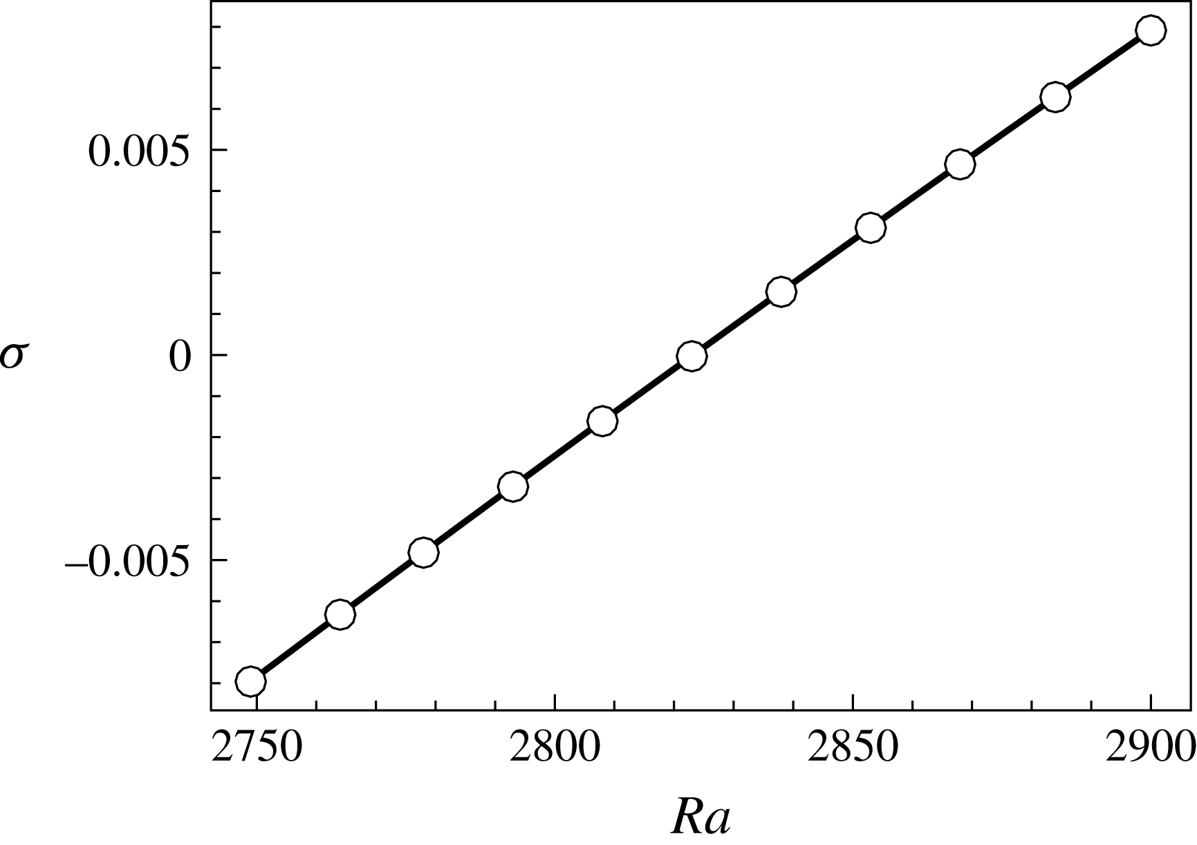
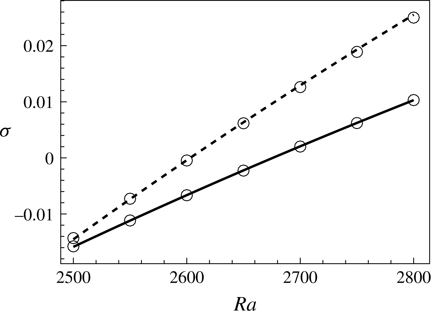
In order to describe various bifurcation processes more faithfully, the amplitude equation up to the seventh order is constructed in practice. To verify the accuracy of weakly nonlinear analysis, the obtained results are compared with those of linear stability analysis and DNS, and qualitative and quantitative agreement is obtained, as shown below. The conduction state is always a solution of the system; correspondingly there is no constant term on the right-hand side of (4.13). For
 $(A,\unicode[STIX]{x1D716})=(1,0.6)$
, the variation of leading disturbance growth rate
 $\unicode[STIX]{x1D70E}$
with
 $Ra$
is obtained by the weakly nonlinear analysis (coefficient
 $g_{1}$
) and compared with results of linear stability analysis, as shown in figure 10. Quantitative agreement is obtained for the two methodologies.
Leading disturbance growth rate
 $\unicode[STIX]{x1D70E}$
computed by weakly nonlinear analysis (line) and linear stability analysis (circles) for
 $(A,\unicode[STIX]{x1D716})=(1,0.6)$
.

In this study the critical eigenmode is generally composed of a certain number of rolls, which are stacked along the horizontal direction. Within the OB approximation, due to symmetries (2.11), the amplitude equation (4.13) is always equivariant under the transformation
 $\unicode[STIX]{x1D6FC}\leftrightarrow -\unicode[STIX]{x1D6FC}$
, indicating
 $g_{2}=0$
. Considering NOB effects, when the critical eigenmode comprises an odd number of rolls, the
 $\unicode[STIX]{x1D6FC}\leftrightarrow -\unicode[STIX]{x1D6FC}$
symmetry is reserved due to the
 $R_{x}$
symmetry and we have
 $g_{2}=0$
. Whereas when an even number of rolls are present, the
 $\unicode[STIX]{x1D6FC}\leftrightarrow -\unicode[STIX]{x1D6FC}$
symmetry is broken due to the breaking of the
 $R_{z}$
symmetry and generally
 $g_{2}\neq 0$
.
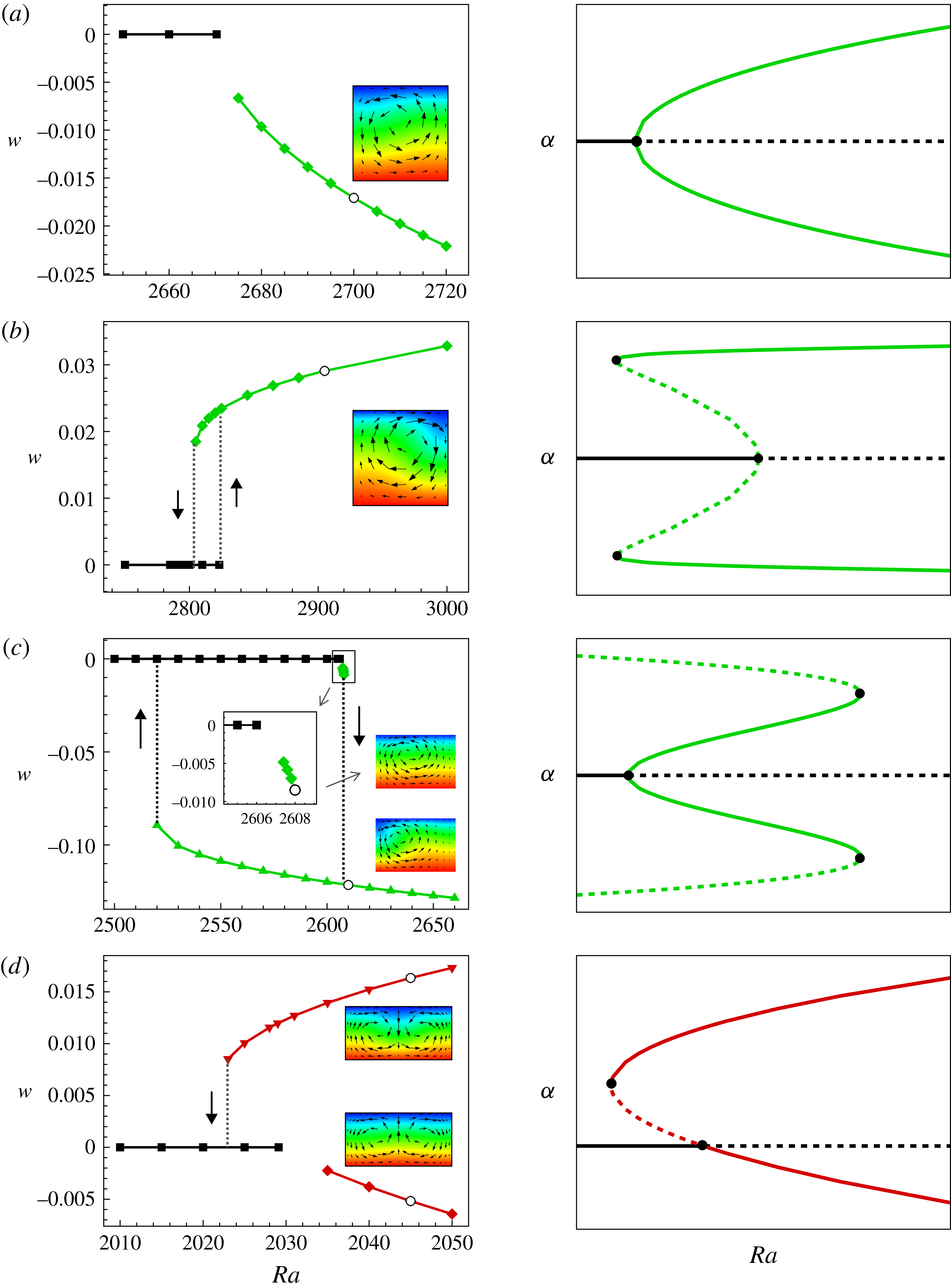
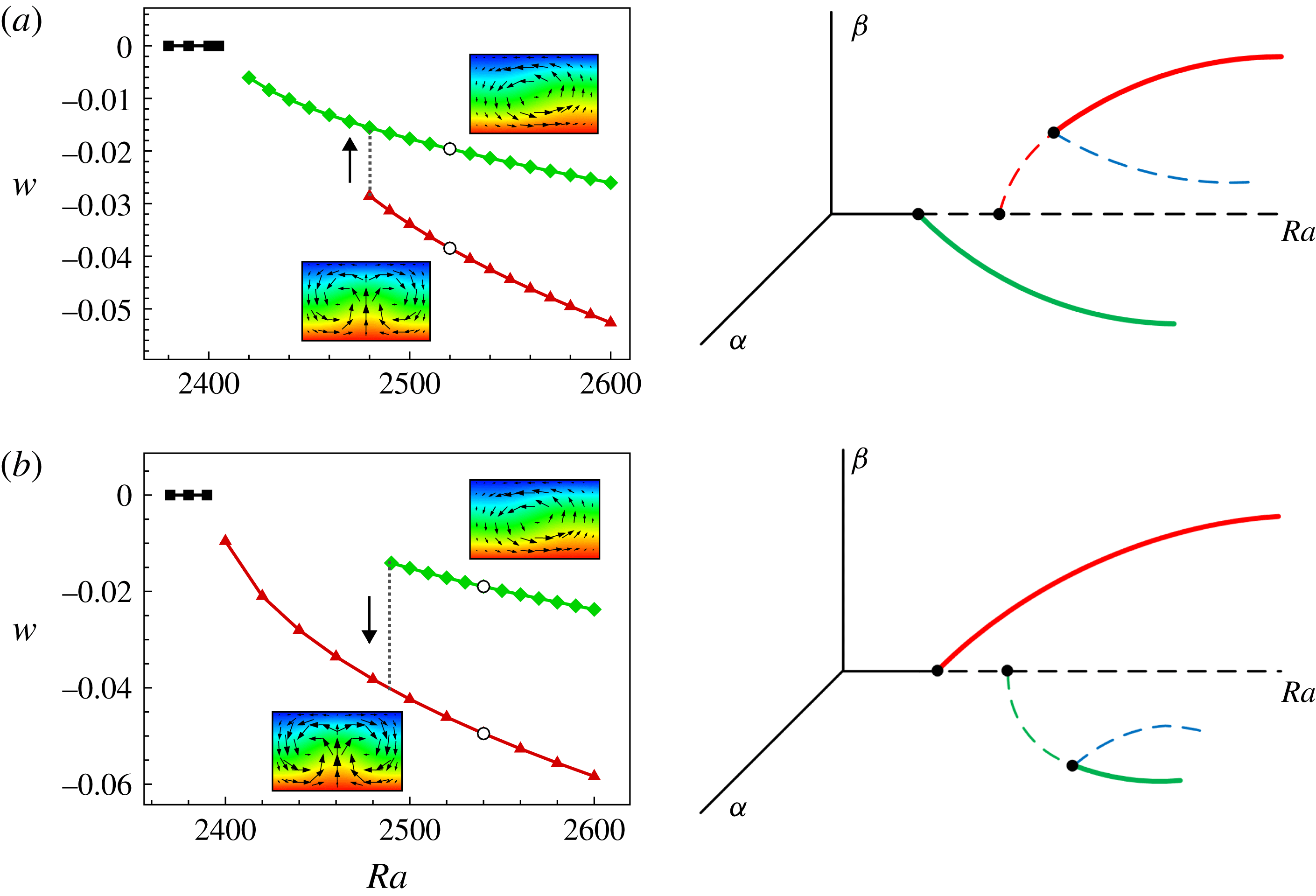
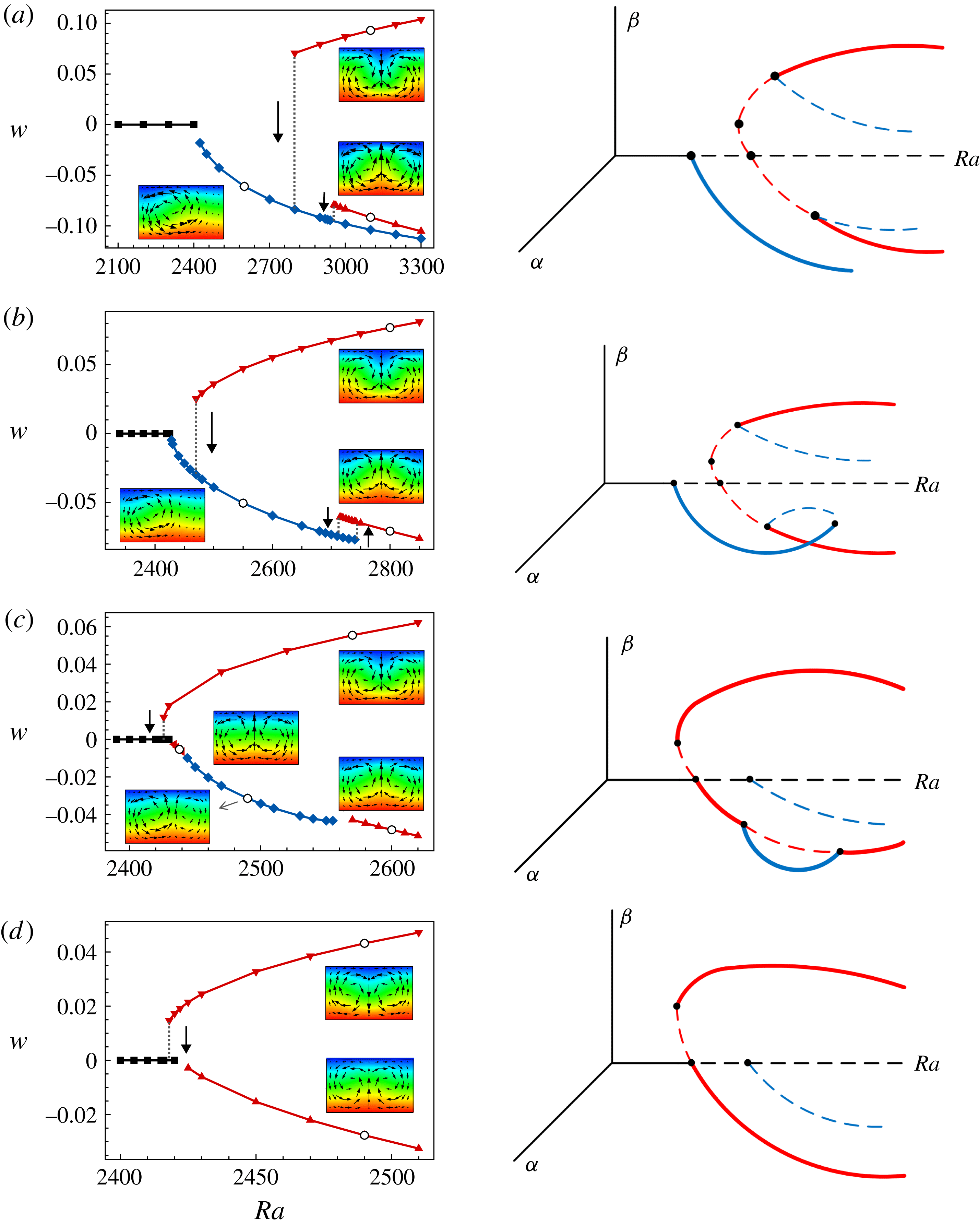
By DNS, bifurcation diagrams at typical parameters
 $(A,\unicode[STIX]{x1D716})$
are obtained, which are depicted in figure 11. Note that only stable solutions are captured by DNS. The vertical velocity component of a monitoring point locating at the mid-plane
 $z=0$
and near the left sidewall is used to characterize various solutions. When different solutions are conjugated with each other with respect to some symmetry, only one of them is shown for simplicity. Discontinuous transitions captured by numerical continuation are marked by solid arrows. We remark that generally very long computation time is needed for numerical solutions to reach steady states near transition points, and in this study accurate critical
 $Ra$
for these transitions are not pursued, which has no qualitative influence on the bifurcation pictures. Schematics of bifurcation regimes based on weakly nonlinear analysis are also depicted in figure 11, where qualitative variations of
 $\unicode[STIX]{x1D6FC}$
with
 $Ra$
are shown. It is observed that bifurcation processes obtained by the two methodologies are qualitatively consistent with each other.
Bifurcation diagrams obtained by DNS (left column) and weakly nonlinear analysis (right column) for codimension-one bifurcations at parameters (a)
 $(A,\unicode[STIX]{x1D716})=(1,0.4)$
, (b)
 $(A,\unicode[STIX]{x1D716})=(1,0.6)$
, (c)
 $(A,\unicode[STIX]{x1D716})=(1.5,0.6)$
and (d)
 $(A,\unicode[STIX]{x1D716})=(2,0.2)$
. In the bifurcation diagrams in the left column, flow fields corresponding to the black circles near them are shown. In the bifurcation diagrams in the right column, stable (unstable) solutions are indicated by solid (dashed) lines. For clarification, one-roll and two-roll solutions are indicated by green and red lines, respectively.

For
 $A\lesssim 1.5$
, the critical eigenmode comprises one dominant roll for various
 $\unicode[STIX]{x1D716}$
and flows with clockwise and anticlockwise rolls are conjugated with each other. In this case we have
 $g_{2}=0$
, indicating that the conduction state loses stability through a perfect pitchfork bifurcation. It is noted that, due to numerical errors,
 $g_{2}$
calculated by weakly nonlinear analysis is not strictly zero. However, near the critical point,
 $g_{2}$
is negligible compared with other terms. Thus, the
 $g_{2}$
term can be discarded and normal form based on symmetry arguments is recovered, as discussed in Carini et al. (Reference Carini, Auteri and Giannetti2015). Analogous symmetry reduction will be performed whenever specific symmetry is present in amplitude equations. The nature of bifurcation due to the unstable one-roll mode is reflected in the sign of Landau coefficient
 $g_{3}$
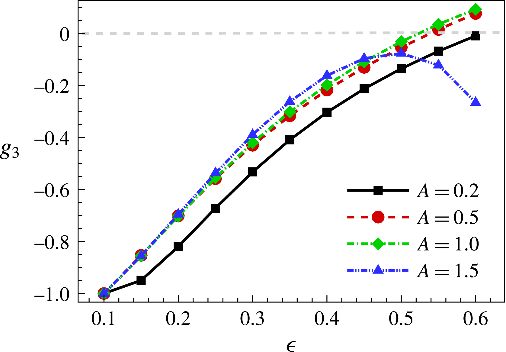
in expressions (4.14). The variations of
 $g_{3}$
with
 $\unicode[STIX]{x1D716}$
for various
 $A$
are illustrated in figure 12. It is observed that, for small
 $A$
(e.g.
 $A=0.2$
),
 $g_{3}<0$
for
 $\unicode[STIX]{x1D716}\leqslant 0.6$
, indicating that convection always appears through a supercritical pitchfork bifurcation. For intermediate
 $A$
(e.g.
 $A=0.5,1$
),
 $g_{3}<0$
for small
 $\unicode[STIX]{x1D716}$
and becomes positive for large
 $\unicode[STIX]{x1D716}$
. Thus, when NOB effects are weak, the pitchfork bifurcation is supercritical, while when NOB effects are strong enough, it becomes subcritical. Similar transition of bifurcation nature due to NOB effects was also observed in a two-dimensional periodic RB system (Fröhlich et al.
Reference Fröhlich, Laure and Peyret1992). For
 $A=1$
, bifurcation diagrams at
 $\unicode[STIX]{x1D716}=0.4$
and 0.6 (before and after the transition point) are shown in figure 11(a,b). For fairly large
 $A$
(e.g.
 $A=1.5$
),
 $g_{3}<0$
for
 $\unicode[STIX]{x1D716}\leqslant 0.6$
and varies non-monotonically with
 $\unicode[STIX]{x1D716}$
. Thus, convection onsets through a supercritical pitchfork bifurcation. However, for large
 $\unicode[STIX]{x1D716}$
the supercritical convection state will disappear through a saddle-node bifurcation near criticality and convection can occur at subcritical
 $Ra$
, as shown in the bifurcation diagrams for
 $(A,\unicode[STIX]{x1D716})=(1.5,0.6)$
in figure 11(c). Note that our weakly nonlinear analysis does not capture faithfully the subcritical stable convection solution, which is not depicted in the schematic bifurcation diagram in figure 11(c).
Variations of Landau coefficient
 $g_{3}$
with
 $\unicode[STIX]{x1D716}$
for various
 $A$
. Normalization is performed so that
 $g_{3}(\unicode[STIX]{x1D716}=0.1)=-1$
.

Here, we also consider a relatively larger aspect ratio case, i.e.
 $A=2$
. In this case the critical eigenmode comprises two horizontally stacked rolls. Within the OB approximation, amplitude equation (4.13) is equivariant under the transformation
 $\unicode[STIX]{x1D6FC}\leftrightarrow -\unicode[STIX]{x1D6FC}$
due to the
 $R_{z}$
symmetry, and solutions with centre plumes flowing upwards and downwards are conjugate with each other. Convection appears through a supercritical pitchfork bifurcation. When NOB effects are taken into account, the
 $R_{z}$
symmetry is broken and generally
 $g_{2}\neq 0$
, as discussed previously. Thus, the bifurcation of convection onset becomes transcritical, as shown in figure 11(d) for
 $(A,\unicode[STIX]{x1D716})=(2,0.2)$
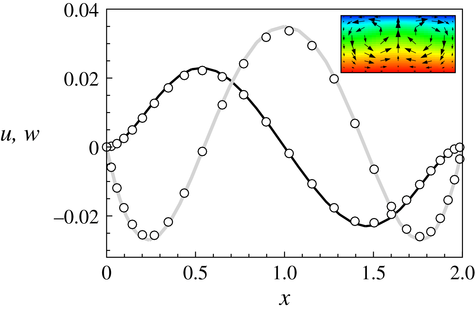
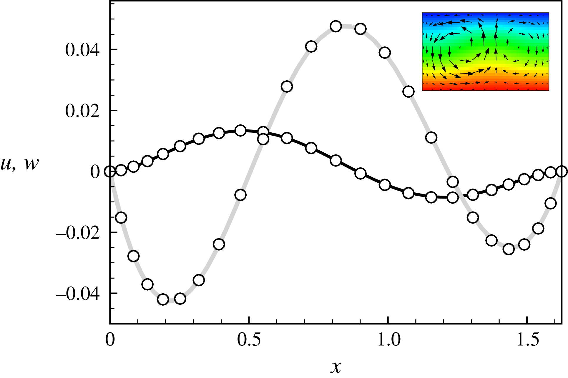
. The two-roll convection solution bifurcating supercritically from the conduction state is obtained by weakly nonlinear analysis for
 $(A,\unicode[STIX]{x1D716},Ra)=(2,0.6,2300)$
(corresponding
 $Ra_{cr}$
is 2210.0084), and velocity profiles along the mid-plane
 $z=0$
are extracted and compared with results of DNS, as shown in figure 13. Good quantitative agreement is obtained.
Profiles along the mid-plane
 $z=0$
of the horizontal velocity component
 $u$
(black line) and vertical component
 $w$
(grey line) of the flow field (inset) constructed by weakly nonlinear analysis for
 $(A,\unicode[STIX]{x1D716},Ra)=(2,0.6,2300)$
. Results of DNS (circles) are also shown for comparison.

4.3 Codimension-two case
At certain parameters
 $(Ra_{cr},A_{cr})$
, eigenmodes comprising
 $n$
and
 $n+1$
rolls can lose stability simultaneously. In this case, two-dimensional amplitude equations are obtained by centre-manifold reduction. The interaction of one- and two-roll modes (
 $n=1$
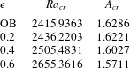
) is investigated as an example to illustrate the possible NOB influences on codimension-two bifurcations. Parameters of codimension-two points for various
 $\unicode[STIX]{x1D716}$
are listed in table 1. It is shown that
 $A_{cr}$
decreases and
 $Ra_{cr}$
increases as NOB effects are increased.
Parameters of codimension-two points for various
 $\unicode[STIX]{x1D716}$
where one- and two-roll modes lose stability simultaneously.

Within the OB approximation, due to symmetries (2.11), two-dimensional amplitude equations should be equivariant under transformations
 $$\begin{eqnarray}\displaystyle \left.\begin{array}{@{}c@{}}R_{x}:(\unicode[STIX]{x1D6FC},\unicode[STIX]{x1D6FD})\leftrightarrow (-\unicode[STIX]{x1D6FC},\unicode[STIX]{x1D6FD}),\\ R_{z}:(\unicode[STIX]{x1D6FC},\unicode[STIX]{x1D6FD})\leftrightarrow (-\unicode[STIX]{x1D6FC},-\unicode[STIX]{x1D6FD}),\end{array}\right\} & & \displaystyle\end{eqnarray}$$
and the general form truncated to the third order reads
 $$\begin{eqnarray}\displaystyle \left.\begin{array}{@{}c@{}}\dot{\unicode[STIX]{x1D6FC}}=g_{10}\unicode[STIX]{x1D6FC}+g_{30}\unicode[STIX]{x1D6FC}^{3}+g_{12}\unicode[STIX]{x1D6FC}\unicode[STIX]{x1D6FD}^{2},\\ \dot{\unicode[STIX]{x1D6FD}}=h_{01}\unicode[STIX]{x1D6FD}+h_{21}\unicode[STIX]{x1D6FC}^{2}\unicode[STIX]{x1D6FD}+h_{03}\unicode[STIX]{x1D6FD}^{3},\end{array}\right\} & & \displaystyle\end{eqnarray}$$
where
 $\unicode[STIX]{x1D6FC}$
and
 $\unicode[STIX]{x1D6FD}$
are the critical amplitudes of one- and two-roll modes, respectively. When NOB effects are taken into account, the
 $R_{z}$
symmetry is broken and the amplitude equations are equivariant only under the transformation
 $(\unicode[STIX]{x1D6FC},\unicode[STIX]{x1D6FD})\leftrightarrow (-\unicode[STIX]{x1D6FC},\unicode[STIX]{x1D6FD})$
. The corresponding amplitude equations truncated to the third order read
 $$\begin{eqnarray}\displaystyle \left.\begin{array}{@{}c@{}}\dot{\unicode[STIX]{x1D6FC}}=g_{10}\unicode[STIX]{x1D6FC}+g_{11}\unicode[STIX]{x1D6FC}\unicode[STIX]{x1D6FD}+g_{30}\unicode[STIX]{x1D6FC}^{3}+g_{12}\unicode[STIX]{x1D6FC}\unicode[STIX]{x1D6FD}^{2},\\ \dot{\unicode[STIX]{x1D6FD}}=h_{01}\unicode[STIX]{x1D6FD}+h_{20}\unicode[STIX]{x1D6FC}^{2}+h_{02}\unicode[STIX]{x1D6FD}^{2}+h_{21}\unicode[STIX]{x1D6FC}^{2}\unicode[STIX]{x1D6FD}+h_{03}\unicode[STIX]{x1D6FD}^{3},\end{array}\right\} & & \displaystyle\end{eqnarray}$$
where
 $$\begin{eqnarray}\displaystyle \left.\begin{array}{@{}c@{}}g_{10}=g_{1,0,0,0}+g_{1,0,1,0}\unicode[STIX]{x1D709}+g_{1,0,0,1}\unicode[STIX]{x1D701}+g_{1,0,2,0}\unicode[STIX]{x1D709}^{2}+g_{1,0,1,1}\unicode[STIX]{x1D709}\unicode[STIX]{x1D701}+g_{1,0,0,2}\unicode[STIX]{x1D701}^{2},\\ g_{11}=g_{1,1,0,0}+g_{1,1,1,0}\unicode[STIX]{x1D709}+g_{1,1,0,1}\unicode[STIX]{x1D701},\\ g_{30}=g_{3,0,0,0},\quad g_{12}=g_{1,2,0,0},\\ h_{01}=h_{0,1,0,0}+h_{0,1,1,0}\unicode[STIX]{x1D709}+h_{0,1,0,1}\unicode[STIX]{x1D701}+h_{0,1,2,0}\unicode[STIX]{x1D709}^{2}+h_{0,1,1,1}\unicode[STIX]{x1D709}\unicode[STIX]{x1D701}+h_{0,1,0,2}\unicode[STIX]{x1D701}^{2},\\ h_{20}=h_{2,0,0,0}+h_{2,0,1,0}\unicode[STIX]{x1D709}+h_{2,0,0,1}\unicode[STIX]{x1D701},\\ h_{02}=h_{0,2,0,0}+h_{0,2,1,0}\unicode[STIX]{x1D709}+h_{0,2,0,1}\unicode[STIX]{x1D701},\\ h_{21}=h_{2,1,0,0},\quad h_{03}=h_{0,3,0,0}.\end{array}\right\} & & \displaystyle\end{eqnarray}$$
In practice, amplitude equations up to the seventh order are constructed. Except for the trivial solution
 $(0,0)$
, equations (4.16) permit pure-mode solutions
 $(\unicode[STIX]{x1D6FC},0),(0,\unicode[STIX]{x1D6FD})$
and mixed-mode solution
 $(\unicode[STIX]{x1D6FC},\unicode[STIX]{x1D6FD})$
with
 $\unicode[STIX]{x1D6FC}\neq 0$
and
 $\unicode[STIX]{x1D6FD}\neq 0$
. Compared with equations (4.16), the amplitude equations (4.17) possess new interaction terms and permit solutions in the form of
 $(0,0)$
,
 $(0,\unicode[STIX]{x1D6FD})$
and
 $(\unicode[STIX]{x1D6FC},\unicode[STIX]{x1D6FD})$
. However, the pure-mode solution
 $(\unicode[STIX]{x1D6FC},0)$
is not permissible due to the presence of the
 $\unicode[STIX]{x1D6FC}^{2}$
term, implying that near criticality the two-roll mode can be excited by the one-roll mode. The growth rates of the one- and two-roll modes for
 $(A,\unicode[STIX]{x1D716})=(1.6,0.6)$
calculated by the weakly nonlinear analysis (coefficients
 $g_{10}$
and
 $h_{01}$
truncated to the first order) and linear stability analysis are shown in figure 14. The results of the two methodologies are in good agreement.
Growth rates of one-roll (solid line) and two-roll (dashed line) modes calculated by the weakly nonlinear analysis for
 $(A,\unicode[STIX]{x1D716})=(1.6,0.6)$
. The results of the linear stability analysis (circles) are also shown for comparison.

Under the OB approximation, bifurcation diagrams near the corresponding codimension-two point are obtained by DNS of the OB equations, which are depicted in figure 15. As mentioned above, when different solutions are conjugated with each other with respect to some symmetry, only one of them is shown for simplicity. The amplitude equations within the OB approximation can be obtained by performing symmetry reduction of those at a very small
 $\unicode[STIX]{x1D716}$
(
 $\unicode[STIX]{x1D716}=10^{-5}$
is used). Schematics of bifurcation regimes based on these amplitude equations are also displayed in figure 15, where the variations of
 $\unicode[STIX]{x1D6FC}$
and
 $\unicode[STIX]{x1D6FD}$
with
 $Ra$
are depicted. Owing to symmetries (4.15), only solutions with
 $\unicode[STIX]{x1D6FC}\geqslant 0$
and
 $\unicode[STIX]{x1D6FD}\geqslant 0$
are shown for simplicity. For clarification, one-roll, two-roll and mixed-mode solutions are indicated by lines of different colours. Specifically, green lines represent the one-roll solutions and lie in the
 $\unicode[STIX]{x1D6FD}=0$
plane, red lines represent the two-roll solutions and lie in the
 $\unicode[STIX]{x1D6FC}=0$
plane, while blue lines represent the mixed-mode solutions and lie out of the
 $\unicode[STIX]{x1D6FC}=0$
and
 $\unicode[STIX]{x1D6FD}=0$
planes. It is observed that the results obtained by the two methodologies are consistent.
When
 $A=1.62<A_{cr,OB}=1.6286$
, as shown in figure 15(a), the one-roll mode loses stability first through a supercritical pitchfork bifurcation and gives rise to a one-roll solution. Subsequently through another supercritical pitchfork bifurcation the two-roll mode becomes unstable and an unstable two-roll solution appears, which gains stability at higher
 $Ra$
and gives rise to an unstable mixed-mode solution. When
 $A=1.64>A_{cr,OB}$
, as shown in figure 15(b), the bifurcation regime is qualitatively similar to that in figure 15(a) when
 $\unicode[STIX]{x1D6FC}$
and
 $\unicode[STIX]{x1D6FD}$
are switched. Mode interactions in a similar convection configuration under the OB approximation have been studied systematically using weakly nonlinear analysis (Metzener Reference Metzener1986).
Bifurcation diagrams obtained by DNS (left column) and weakly nonlinear analysis (right column) within the OB approximation at (a)
 $A=1.62<A_{cr,OB}$
and (b)
 $A=1.64>A_{cr,OB}$
. In the bifurcation diagrams (right column), stable (unstable) solutions are indicated by solid (dashed) lines. For clarification, one-roll, two-roll and mixed-mode solutions are indicated by green, red and blue lines, respectively.

Bifurcation diagrams obtained by DNS (left column) and weakly nonlinear analysis (right column) for
 $\unicode[STIX]{x1D716}=0.2$
and (a)
 $A=1.58<A_{cr}$
, (b)
 $A=1.61<A_{cr}$
, (c)
 $A=1.625>A_{cr}$
and (d)
 $A=1.63>A_{cr}$
. In the bifurcation diagrams in the right column, stable (unstable) solutions are indicated by solid (dashed) lines. For clarification, two-roll and mixed-mode solutions are indicated by red and blue lines, respectively.

On account of NOB effects, the
 $(\unicode[STIX]{x1D6FC},\unicode[STIX]{x1D6FD})\leftrightarrow (-\unicode[STIX]{x1D6FC},-\unicode[STIX]{x1D6FD})$
symmetry of the amplitude equations (4.17) is broken and the interaction of one- and two-roll modes is expected to be qualitatively different from the OB case. Here we choose the
 $\unicode[STIX]{x1D716}=0.2$
case as an example to illustrate this point. The bifurcation diagrams obtained by both DNS and weakly nonlinear analysis are shown in figure 16. In the bifurcation diagrams obtained by the weakly nonlinear analysis, considering the
 $(\unicode[STIX]{x1D6FC},\unicode[STIX]{x1D6FD})\leftrightarrow (-\unicode[STIX]{x1D6FC},\unicode[STIX]{x1D6FD})$
symmetry, only solutions with
 $\unicode[STIX]{x1D6FC}\geqslant 0$
are shown for simplicity. The bifurcation diagrams for
 $A<A_{cr}=1.6221$
are shown in figure 16(a,b). When
 $A=1.58$
, as shown in figure 16(a), the one-roll mode loses stability first through a supercritical pitchfork bifurcation and simultaneously a stable two-roll mode is excited due to NOB effects. Thus, a stable mixed-mode solution appears. Subsequently unstable two-roll solutions appear through a transcritical bifurcation and gain stability after pitchfork bifurcations. When
 $A=1.61$
, relatively closer to
 $A_{cr}$
, a qualitative change of the bifurcation regime is observed as shown in figure 16(b). The stable mixed-mode solution disappears through a saddle-node bifurcation near criticality, and the corresponding solution branch is connected with a two-roll branch through a mixed-mode branch. Thus, near convection onset a stable mixed-mode solution of a finite
 $Ra$
range appears and a hysteresis loop is present.
Bifurcation diagrams for
 $A>A_{cr}$
are shown in figure 16(c,d). When
 $A=1.625$
, as shown in figure 16(c), the conduction state first gives rise to two-roll solutions through a transcritical bifurcation. The subcritical one disappears after a saddle-node bifurcation as
 $Ra$
is decreased. The supercritical one loses and gains stability as
 $Ra$
is increased and gives rise to a stable mixed-mode solution in a finite range of
 $Ra$
. As the one-roll mode becomes unstable, an unstable mixed-mode solution appears. The flow field of the stable mixed-mode solution at
 $Ra=2490$
is obtained by weakly nonlinear analysis, and velocity profiles along the mid-plane
 $z=0$
are extracted and compared with results of DNS, as shown in figure 17. Good quantitative agreement is obtained. When
 $A=1.63$
, away from
 $A_{cr}$
, the bifurcation regime becomes simpler as shown in figure 16(d). Near convection onset the supercritical two-roll solution remains stable and no stable mixed-mode solution is found.
Profiles along the mid-plane
 $z=0$
of the horizontal velocity component
 $u$
(black line) and vertical component
 $w$
(grey line) of the flow field (inset) constructed by weakly nonlinear analysis for
 $(A,\unicode[STIX]{x1D716},Ra)=(1.625,0.2,2490)$
. Results of DNS (circles) are also shown for comparison.

Overall, near codimension-one criticality, depending on the symmetry of the critical eigenmode and the intensity of NOB effects, the bifurcation process can be qualitatively different from the OB case. In the codimension-two case, the interaction of two critical eigenmodes is also qualitatively influenced by NOB effects. In both cases, bifurcation characteristics depend sensitively on the confinement of sidewalls. Near criticality, both stable and unstable solutions can be captured by weakly nonlinear analysis, which is useful for organizing and understanding the DNS results.
5 Summary and discussion
In this study, the NOB influences on flow instabilities and bifurcation processes of RB convection in two-dimensional rigid cavities of finite aspect ratios are examined. The working fluid is air. Subject to a large temperature difference, the variations of fluid properties and flow compressibility are significant, and the low-Mach-number equations with acoustic waves filtered are employed to deal with such NOB effects.
Flow instabilities and bifurcation processes are found to be qualitatively and quantitatively influenced by NOB effects. Firstly, through linear stability analysis, the loss of the reflection symmetry of the critical eigenmode about the horizontal mid-plane is observed under NOB conditions. It is also found that both the disturbance growth rate
 $\unicode[STIX]{x1D70E}$
and the critical Rayleigh number
 $Ra_{cr}$
vary with
 $\unicode[STIX]{x1D716}$
with leading-order corrections
 ${\sim}\unicode[STIX]{x1D716}^{2}$
generally, due to the intrinsic symmetry of the system.
Secondly, by performing a perturbation expansion of the LSE in
 $\unicode[STIX]{x1D716}$
, the influences of weak NOB effects on critical quantities are identified. It is interesting that NOB effects possess the dual nature of stabilizing and destabilizing, which relies on aspect ratio. In relatively wide cavities, NOB effects are stabilizing, while they are destabilizing in narrow cavity systems. A detailed budget analysis of disturbance kinetic energy shows that contributions of compressibility, viscosity and buoyancy vary with
 $\unicode[STIX]{x1D716}$
with leading-order corrections
 ${\sim}\unicode[STIX]{x1D716}^{2}$
. Considering NOB effects, viscosity and buoyancy actions are weakened in narrow cavities, whilst being enhanced in wide cavities. Compressibility has both destabilizing and stabilizing effects under NOB conditions. Compared with compressibility and buoyancy, viscosity action is generally more sensitive to NOB effects and plays a dominate role in the NOB influences on disturbance growth rate.
Finally, amplitude equations are derived based on centre-manifold reduction, and then the bifurcation nature of convection onset is studied for both codimension-one and -two cases. For the codimension-one case, bifurcation characteristics are sensitive to the symmetry of the critical eigenmode and the intensity of NOB effects. When
 $A\lesssim 1.5$
, the one-roll mode becomes unstable first. In this aspect ratio range, when
 $A$
is relatively small, convection always appears through a supercritical pitchfork bifurcation for
 $\unicode[STIX]{x1D716}\leqslant 0.6$
. For intermediate
 $A$
, the pitchfork bifurcation of convection onset is supercritical when NOB effects are weak and becomes subcritical for strong enough NOB effects. For fairly large
 $A$
, although the conduction state loses stability through a supercritical pitchfork bifurcation, convection can occur at subcritical
 $Ra$
for large
 $\unicode[STIX]{x1D716}$
. In the case of
 $A=2$
, the two-roll mode firstly becomes unstable and the bifurcation of convection onset becomes transcritical under NOB conditions. Moreover, for the codimension-two case, NOB effects lead to new interaction terms in the normal form of amplitude equations. The bifurcation regimes induced by the interaction of one- and two-roll modes are qualitatively influenced by NOB effects. In both codimension-one and -two cases, bifurcation processes are sensitive to the confinement of sidewalls.
Compared with previous studies of NOB influences on RB instabilities, which mainly focused on spatial extended systems, it is shown in this work that flows in cavities of different aspect ratios can respond differently to the NOB effects, in both the linear and nonlinear regimes. The combination of symmetry breaking due to NOB effects and selection of flow structures by geometry confinement can have non-trivial influences on flow evolutions.
While a two-dimensional configuration is adopted in this study, it is expected that some of the results obtained can also be relevant in three-dimensional convection. In three-dimensional configuration, though the two-dimensional convection structures of fluid flows assumed here cannot be realized strictly, the convection rolls can line up parallel to a pair of sidewalls and possess nearly two-dimensional structures near the threshold of convection onset. Besides, when the cavity dimension along the axis of convection rolls is not too small, it is expected that the centre of flow will not be influenced greatly by the front walls and the results of two-dimensional convection can be applied. When fully three-dimensional flow structures are developed, the results of the current work cannot be applied directly and a detailed investigation is needed to explore the three-dimensional flow dynamics. However, it is expected that phenomena similar to those we observed, e.g. the qualitative change of bifurcation nature with aspect ratio under NOB conditions, can also appear in fully three-dimensional problems.
In this study, we focused on the NOB effects of air due to a large temperature difference in two-dimensional cavities of finite aspect ratios. Linear and weakly nonlinear stability analyses are in principle important methods to obtain details that are useful for organizing and understanding the DNS results near instability thresholds. It is of interest to extend the present methods to study the NOB effects of different media (e.g. water, glycerol) and flow configurations of different symmetries (e.g. cylinder, annulus).
Acknowledgements
This work is supported by the National Natural Science Foundation of China (grant nos 11572314, 11232011, 11621202 and 11642020), the Science Challenge Project (no. JCKY2016212A501) and the Fundamental Research Funds for the Central Universities.
Appendix A
In equation (3.2) the linear operators
 $\boldsymbol{C}$
and
 $\boldsymbol{L}$
are
 $$\begin{eqnarray}\displaystyle \boldsymbol{C}=\left[\begin{array}{@{}cccc@{}}\unicode[STIX]{x1D644} & 0 & 0 & 0\\ 0 & \unicode[STIX]{x1D644} & 0 & 0\\ 0 & 0 & \unicode[STIX]{x1D644}-\unicode[STIX]{x1D6E4}\overline{S}p_{L} & 0\\ 0 & 0 & \unicode[STIX]{x1D644}-\overline{S}p_{L} & 0\end{array}\right],\quad \boldsymbol{L}=\left[\begin{array}{@{}cccc@{}}L_{11} & L_{12} & 0 & L_{14}\\ L_{21} & L_{22} & L_{23} & L_{24}\\ 0 & L_{32} & L_{33} & 0\\ L_{41} & L_{42} & 0 & 0\end{array}\right], & & \displaystyle\end{eqnarray}$$
and the components of
 $\boldsymbol{L}$
read as follows:
 $$\begin{eqnarray}\displaystyle \left.\begin{array}{@{}c@{}}\displaystyle L_{11}=\sqrt{\frac{Pr}{Ra}}\overline{S}\left(\frac{4}{3}M_{11}+M_{22}\right),\quad L_{12}=\sqrt{\frac{Pr}{Ra}}\overline{S}\left(-\frac{2}{3}M_{12}+M_{21}\right),\\ \displaystyle L_{14}=-\overline{S}\frac{\unicode[STIX]{x2202}}{\unicode[STIX]{x2202}x},\quad L_{21}=\sqrt{\frac{Pr}{Ra}}\overline{S}\left(-\frac{2}{3}M_{21}+M_{12}\right),\\ \displaystyle L_{22}=\sqrt{\frac{Pr}{Ra}}\overline{S}\left(M_{11}+\frac{4}{3}M_{22}\right),\quad L_{23}=-\frac{\text{d}\overline{\unicode[STIX]{x1D70B}}}{\text{d}z}S_{L}+\frac{1}{2\unicode[STIX]{x1D716}}S_{L},\\ \displaystyle L_{24}=-\overline{S}\frac{\unicode[STIX]{x2202}}{\unicode[STIX]{x2202}z},\quad L_{32}=-\frac{\text{d}\overline{T}}{\text{d}z},\\ \displaystyle L_{33}=\frac{1}{\sqrt{PrRa}}\overline{S}\left[\frac{\unicode[STIX]{x2202}}{\unicode[STIX]{x2202}x}\left(\overline{k}\frac{\unicode[STIX]{x2202}}{\unicode[STIX]{x2202}x}\right)+\frac{\unicode[STIX]{x2202}}{\unicode[STIX]{x2202}z}\left(\frac{\text{d}\overline{T}}{\text{d}z}k_{L}\right)+\frac{\unicode[STIX]{x2202}}{\unicode[STIX]{x2202}z}\left(\overline{k}\frac{\unicode[STIX]{x2202}}{\unicode[STIX]{x2202}z}\right)\right],\\ \displaystyle L_{41}=\overline{T}\frac{\unicode[STIX]{x2202}}{\unicode[STIX]{x2202}x},\quad L_{42}=\overline{T}\frac{\unicode[STIX]{x2202}}{\unicode[STIX]{x2202}z}-\frac{\text{d}\overline{T}}{\text{d}z}.\end{array}\right\} & & \displaystyle\end{eqnarray}$$
In the expressions above,
 $\unicode[STIX]{x1D644}$
is the identity operator,
 $\overline{S}=1/\overline{\unicode[STIX]{x1D70C}}$
,
 $M_{ij}=\unicode[STIX]{x2202}(\overline{\unicode[STIX]{x1D707}}(\unicode[STIX]{x2202}/\unicode[STIX]{x2202}x_{j}))/\unicode[STIX]{x2202}x_{i}$
,
 $k_{L}=\text{d}k/\text{d}T|_{\overline{T}}$
and
 $$\begin{eqnarray}\displaystyle \left.\begin{array}{@{}c@{}}\displaystyle p_{L}(\tilde{T})=\overline{p}\int _{V}\frac{\,\overline{\unicode[STIX]{x1D70C}}\,}{\,\overline{T}\,}\tilde{T}\,\text{d}V,\\ \displaystyle S_{L}(\tilde{T})=\overline{S}\left(\frac{\tilde{T}}{\,\overline{T}\,}-\int _{V}\frac{\,\overline{\unicode[STIX]{x1D70C}}\,}{\,\overline{T}\,}\tilde{T}\,\text{d}V\right).\end{array}\right\} & & \displaystyle\end{eqnarray}$$
Appendix B
Operators
 $\boldsymbol{A}$
and
 $\boldsymbol{B}$
in (3.8) are
 $$\begin{eqnarray}\displaystyle \boldsymbol{A}=\left[\begin{array}{@{}cccc@{}}A_{11} & A_{12} & 0 & 0\\ A_{21} & A_{22} & 0 & 0\\ 0 & 0 & A_{33} & 0\\ 0 & 0 & 0 & 0\end{array}\right],\quad \boldsymbol{B}=\left[\begin{array}{@{}cccc@{}}0 & 0 & 0 & B_{14}\\ 0 & 0 & B_{23} & B_{24}\\ 0 & B_{32} & 0 & 0\\ B_{41} & B_{42} & 0 & 0\end{array}\right], & & \displaystyle\end{eqnarray}$$
where
 $$\begin{eqnarray}\displaystyle \left.\begin{array}{@{}c@{}}A_{11}=\frac{4}{3}M_{11}+M_{22},\quad A_{12}=-\frac{2}{3}M_{12}+M_{21},\quad A_{21}=M_{12}-\frac{2}{3}M_{21},\\ \displaystyle A_{22}=M_{11}+\frac{4}{3}M_{22},\quad A_{33}=\frac{1}{Pr}\left(\frac{\unicode[STIX]{x2202}^{2}}{\unicode[STIX]{x2202}x^{2}}+\frac{\unicode[STIX]{x2202}^{2}}{\unicode[STIX]{x2202}z^{2}}\right),\quad B_{14}=\frac{\unicode[STIX]{x2202}}{\unicode[STIX]{x2202}x},\\ \displaystyle B_{23}=-\frac{1}{2}g_{L},\quad B_{24}=\frac{\unicode[STIX]{x2202}}{\unicode[STIX]{x2202}z},\quad B_{32}=-2,\quad B_{41}=\frac{\unicode[STIX]{x2202}}{\unicode[STIX]{x2202}x},\quad B_{42}=\frac{\unicode[STIX]{x2202}}{\unicode[STIX]{x2202}z},\end{array}\right\} & & \displaystyle\end{eqnarray}$$
with
 $g_{L}(\tilde{T})=\tilde{T}-(1/V)\int _{V}\tilde{T}\,\text{d}V$
.