1 Introduction
In wall-bounded flows, power must be supplied to the flow in order to overcome dissipation by means of viscous and pressure drag. Increasing energy costs motivate the search for methods to reduce the power consumption and one way to achieve this goal is to reduce drag. Techniques resulting in the reduction of pressure drag are well established while methods that result in the reduction of friction drag are still being actively researched.
It is well known that turbulent flows have higher skin friction than laminar flows and, thus, one of the popular drag-reducing techniques relies on the delay of the laminar–turbulent transition. Once the turbulent flow has been established, its structure can be rearranged using either passive or active devices with the hope that the new flow will be characterized by a smaller skin friction.
Since the beginning of modern fluid mechanics, it has been commonly believed that the drag on a smooth surface is always lower than that on a rough surface (Hagen Reference Hagen1854; Darcy Reference Darcy1857; Nikuradse Reference Nikuradse1933; Moody Reference Moody1944). This is actually not the case, as documented through the development of special drag-reducing surface topographies; see a recent review in García-Mayoral & Jiménez (Reference García-Mayoral and Jiménez2011). The advantage of such topographies is in the passive character of the drag reduction which eliminates the energy costs associated with the use of active techniques (Choi, Jukes & Whalley Reference Choi, Jukes and Whalley2011; Quadrio Reference Quadrio2011). The physics of turbulent drag reduction is well summarized by Kim (Reference Kim2011).
One of the early passive methods of drag reduction was the large eddy break up (LEBU) method (Savill & Mumford Reference Savill and Mumford1988). This method usually employs small flat or airfoil shaped ribbons within the boundary layer. The wake behind such ribbons interacts with the turbulent boundary layer and suppresses the velocity normal to the wall (Balakumar & Widnall Reference Balakumar and Widnall1986; Graham Reference Graham1998), resulting in a reduction in turbulent motion and skin friction immediately downstream of the devices. The drag reduction is up to 40 % as reported by Sahlin, Johansson & Alfredsson (Reference Sahlin, Johansson and Alfredsson1988), however there is a large spread and doubt in the drag reduction value due to the difficulty and inaccuracies of indirect measuring methods at relatively low Reynolds numbers (Savill & Mumford Reference Savill and Mumford1988). In addition, drag reduction at practically high Reynolds numbers seems implausible as LEBU devices reduce skin friction via breaking up the large-scale motions whose size becomes much smaller than the devices. This is supported by the direct force measurements conducted by Sahlin, Alfredsson & Johansson (Reference Sahlin, Alfredsson and Johansson1986), Sahlin et al. (Reference Sahlin, Johansson and Alfredsson1988) at Reynolds numbers up to 260 000.
Nature provides numerous examples of special drag-reducing surface topographies. Shark (superorder Selachimorpha) is one of the fastest swimming fish, whose speed can exceed
 $40{-}50~\text{km}~\text{h}^{-1}$
(the ‘shortfin mako shark’ and the ‘great white shark’) during hunting. Microscopic examination of shark skin showed that it consists of small jagged and overlapping scales with a valley/ridge structure (denticle) in the flow direction. The scales are believed to disrupt the turbulent flow structures and in this manner they reduce the drag (Bechert, Bruse & Hage Reference Bechert, Bruse and Hage2000; Dean & Bhushan Reference Dean and Bhushan2010). Riblets, inspired by the shark skin, have the form of streamwise microgrooves and represent one of the well-known skin-friction reducing methods (Walsh Reference Walsh1980, Reference Walsh1983). The structure of riblets is different from shark skin, as the former has a continuous geometry while the latter is discrete in the streamwise direction. Riblets generally have two types of cross-section: wedge-like and blade-like (see Sudo et al.
Reference Sudo, Tsuyuki, Ito and Ikohagi2002). The height and spacing expressed in terms of wall units for the ‘wedge’ or ‘blade’ are approximately 10–30. It is generally accepted that the highest drag reduction that can be achieved in turbulent channel flow by riblets is approximately 7 %–9 % (Bechert et al.
Reference Bechert, Bruse, Hage, Van Der Hoeven and Hoppe1997; Itoh et al.
Reference Itoh, Tamano, Iguchi, Yokota, Akino, Hino and Kubo2006). The direct numerical simulations of Choi, Moin & Kim (Reference Choi, Moin and Kim1993) demonstrated that the drag reduction is achieved by depressing the velocity and vorticity fluctuations as well as the Reynolds stresses. See also Bechert & Bartenwerfer (Reference Bechert and Bartenwerfer1989) and Choi (Reference Choi1989).
Sirovich & Karlsson (Reference Sirovich and Karlsson1997) employed randomly patterned ‘V’ protrusions and experimentally found an approximately 10 % drag reduction in turbulent channel flow (
 $15\,000<Re_{2H}<40\,000$
) as compared to a smooth channel. The experimental and numerical results obtained by Sagong et al. (Reference Sagong, Kim, Choi, Jeon and Choi2008), however, showed that the drag on randomly patterned ‘V’ protrusions is increased by 0 %–15 %. The disagreement among researchers as to whether ‘V’ protrusions induce drag reduction led Chen, Chew & Khoo (Reference Chen, Chew and Khoo2010) to conduct numerical simulations for Reynolds numbers
 $10\,000<Re_{2H}<40\,000$
. Their results showed that neither the random nor aligned ‘V’ protrusions can reduce drag in a fully developed turbulent channel flow.
Another alternative is offered by the so-called super-hydrophobic effect (Rothstein Reference Rothstein2010) which results from a combination of the hydrophobicity of the liquid and surface material and surface topography. When a super-hydrophobic surface is submerged inside a liquid, gas bubbles become trapped in surface micro-pores effectively reducing the shear stress experienced by the liquid, as shear between the liquid and the solid is replaced by shear between the liquid and the gas, with the research being inspired by the unique water-repellent properties of the lotus leaf (Barthlott & Neinhuis Reference Barthlott and Neinhuis1997). The drag reducing abilities can be increased by correctly shaping the surface pores/roughness (Samaha, Tafreshi & Gad-el Hak Reference Samaha, Tafreshi and Gad-el Hak2011) and by increasing hydrophobicity through changes in surface chemistry (Gao & McCarthy Reference Gao and McCarthy2006; Quéré Reference Quéré2008; Reyssat, Yeomans & Quéré Reference Reyssat, Yeomans and Quéré2008; Zhang et al. Reference Zhang, Shi, Niu, Jiang and Wang2008; Zhou et al. Reference Zhou, Li, Wu, Zhou and Cai2011). While laminar drag reduction due to the super-hydrophobic effect is well documented (Ou, Perot & Rothstein Reference Ou, Perot and Rothstein2004; Ou & Rothstein Reference Ou and Rothstein2005; Joseph et al. Reference Joseph, Cottin-Bizonne, Benoit, Ybert, Journet, Tabeling and Bocquet2006; Truesdell et al. Reference Truesdell, Mammoli, Vorobieff, van Swol and Brinker2006), techniques which rely on this effect to reduce turbulent drag are still being developed (Daniello, Waterhouse & Rothstein Reference Daniello, Waterhouse and Rothstein2009; Martell, Perot & Rothstein Reference Martell, Perot and Rothstein2009; Park, Park & Kim Reference Park, Park and Kim2013).
Dimpled surfaces, which were first designed and have been studied extensively for heat transfer enhancement (Burgess, Oliveira & Ligrani Reference Burgess, Oliveira and Ligrani2003), may also have the potential to reduce drag (Alekseev et al. Reference Alekseev, Gachechiladze, Kiknadze and Oleinikov1998). Conflicting views on their drag reduction capability are reported; some studies (Alekseev et al. Reference Alekseev, Gachechiladze, Kiknadze and Oleinikov1998; Veldhuis & Vervoort Reference Veldhuis and Vervoort2009) reported dramatic drag reduction even up to 10%–20 % compared to flat surfaces, while others (Lienhart, Breuer & Köksoy Reference Lienhart, Breuer and Köksoy2008; Tay, Khoo & Chew Reference Tay, Khoo and Chew2015) reported little (approximately 3 %) to no drag reduction in both external and internal turbulent flow. Tay et al. (Reference Tay, Khoo and Chew2015) revealed that the turbulent motion on the small scales is suppressed by the streamwise vorticity generated on the dimpled surfaces, leading to the reduction of turbulent skin friction. It was also shown that, although increasing dimple depth further reduces skin friction, the net drag reduction may drop because of the significant increase in form drag due to the flow separation.
Besides the three-dimensional dimples, another macro-scale device is represented by two-dimensional grooves in channel flow. In order to examine the drag over such surfaces, Mohammadi & Floryan (Reference Mohammadi and Floryan2013b ) investigated such grooves of arbitrary shape with an arbitrary orientation in laminar flow. It was found that transverse grooves produce the highest drag while longitudinal grooves produce the lowest drag. Drag reduction was reported for longitudinal grooves with long wavelengths, in spite of an increase in the wetted surface area. This reduction was attributed to the redistribution of the mass flow, with the largest mass flow taking place in the widest channel opening. It was found that short-wavelength grooves increase the drag when compared to the smooth channel. A detailed study of grooves of various shapes can be found in Mohammadi & Floryan (Reference Mohammadi and Floryan2015). Moradi & Floryan (Reference Moradi and Floryan2013) have shown that similar grooves reduce laminar drag in an annulus flow. It is possible that the same grooves may be able to reduce turbulent drag.
Several active methods have been developed for drag reduction and they are briefly reviewed for completeness. Spanwise in-plane wall oscillations have the potential for up to 40 % drag reduction (Quadrio Reference Quadrio2011). The creation of such waves using plasma actuation is discussed in Choi et al. (Reference Choi, Jukes and Whalley2011). Considering the energy needed to drive the oscillation, the maximum net energy saving is approximately 5 %–10 %. Upstream travelling waves produced by suction/blowing can reduce the turbulent drag to below that for the laminar flow (Min et al. Reference Min, Kang, Speyer and Kim2006). A similar effect is achieved by elastic wall deformation waves (Hoepffner & Fukagata Reference Hoepffner and Fukagata2009). Schoppa & Hussain (Reference Schoppa and Hussain1998) showed that counter-rotating streamwise vortices produced by colliding wall jets were able to reduce drag by 20 %. Iuso et al. (Reference Iuso, Onorato, Spazzini and Di Cicca2002) experimentally showed that counter-rotating vortex pairs, which are generated by jet injection, reduce the mean skin friction by 15 %.
Though considerable effort has been expended to develop various potential drag-reducing techniques, techniques that are readily applicable in engineering practice are yet to be identified. Riblets, ‘V’ protrusions and super-hydrophobic surfaces containing micro-scale structures are difficult to manufacture and maintain. Active methods need additional power, which reduces their efficiency and creates hardware needs which can be difficult to overcome. Thus, there is a need to design a novel device which is passive (no additional energy input), has a macro-scale format (easy to manufacture and maintain) and still has a high level of drag reduction (no less than that of riblets).
Considering the advantages of macro-scale surface modifications over micro-scale modifications (e.g. riblets, superhydrophobic surfaces, etc), the objective of this analysis is to carry out a detailed investigation of turbulent flows in channels with surfaces modified with longitudinal grooves of arbitrary shape and wavelength. It is known that grooves with long wavelengths are able to reduce the laminar drag. Our intent is to determine if there are classes of such grooves which are able to reduce the turbulent drag, to explore in detail the performance of such grooves and to identify the possible mechanism(s) responsible for the drag reduction. The drag-reducing potential is measured by comparing the discharge through the grooved channel with the discharge through a smooth channel when both channels are exposed to the same pressure gradient.
This paper is organized as follows. The channel geometry and the governing equations are introduced in § 2. The analytical results for the laminar flows are presented in § 3. Turbulent flows are investigated numerically in § 4. The concluding remarks are provided in § 5.
2 Problem formulation
2.1 Channel geometry
Consider fluid flow driven by a known pressure gradient through a channel extending to
 $\pm \infty$
in the
 $x$
-direction bounded by walls fitted with straight grooves parallel to the flow direction (see figure 1) and of arbitrary shape in the spanwise
 $z$
-direction. The channel geometry is described using Fourier expansions of the form
 $$\begin{eqnarray}\displaystyle & \displaystyle y_{L}(z)=-1+\mathop{\sum }_{m=-N_{A}}^{m=N_{A}}H_{L}^{(m)}\text{e}^{\text{i}m{\it\alpha}z}, & \displaystyle\end{eqnarray}$$
 $$\begin{eqnarray}\displaystyle & \displaystyle y_{U}(z)=1+\mathop{\sum }_{m=-N_{A}}^{m=N_{A}}H_{U}^{(m)}\text{e}^{\text{i}m{\it\alpha}z}, & \displaystyle\end{eqnarray}$$
 $L$
and
 $U$
refer to the lower and upper walls, respectively,
 ${\it\lambda}=2{\rm\pi}/{\it\alpha}$
denotes the groove wavelength,
 ${\it\alpha}$
stands for the groove wavenumber,
 $H_{L}^{(m)}=H_{L}^{(-m)\ast \ast }$
and
 $H_{U}^{(m)}=H_{U}^{(-m)\ast \ast }$
are the reality conditions, double stars denote the complex conjugates,
 $N_{A}$
represents the number of Fourier modes required to describe the geometry and the half-channel height
 $H^{\ast }$
of the reference smooth channel has been used as the length scale. The objective of this analysis is to describe the effects of the flow modulations on the channel discharge and, accordingly, it is assumed that the mean openings of the grooved and the reference smooth channels are the same, i.e.
 $H_{L}^{(0)}=H_{U}^{(0)}=0$
.
Sketch of the flow configuration.

2.2 Field equations
It is assumed that the introduction of the grooves does not affect the mean streamwise pressure gradient and, thus, the pressure is represented as
 $p(x,y,z,t)=-x+p^{\prime }(x,y,z,t)+\text{const}$
. The discharge is, however, affected and its evaluation requires solving the field equations of the form
 $$\begin{eqnarray}\displaystyle & \displaystyle \frac{\partial u}{\partial x}+\frac{\partial v}{\partial y}+\frac{\partial w}{\partial z}=0, & \displaystyle\end{eqnarray}$$
 $$\begin{eqnarray}\displaystyle & \displaystyle \frac{\partial u}{\partial t}+\frac{\partial (uu)}{\partial x}+\frac{\partial (uv)}{\partial y}+\frac{\partial (uw)}{\partial z}=1-\frac{\partial p^{\prime }}{\partial x}+\frac{1}{Re_{{\it\tau}}}\left(\frac{\partial ^{2}u}{\partial x^{2}}+\frac{\partial ^{2}u}{\partial y^{2}}+\frac{\partial ^{2}u}{\partial z^{2}}\right), & \displaystyle\end{eqnarray}$$
 $$\begin{eqnarray}\displaystyle & \displaystyle \frac{\partial v}{\partial t}+\frac{\partial (vu)}{\partial x}+\frac{\partial (vv)}{\partial y}+\frac{\partial (vw)}{\partial z}=-\frac{\partial p^{\prime }}{\partial y}+\frac{1}{Re_{{\it\tau}}}\left(\frac{\partial ^{2}v}{\partial x^{2}}+\frac{\partial ^{2}v}{\partial y^{2}}+\frac{\partial ^{2}v}{\partial z^{2}}\right), & \displaystyle\end{eqnarray}$$
 $$\begin{eqnarray}\displaystyle & \displaystyle \frac{\partial w}{\partial t}+\frac{\partial (wu)}{\partial x}+\frac{\partial (wv)}{\partial y}+\frac{\partial (ww)}{\partial z}=-\frac{\partial p^{\prime }}{\partial z}+\frac{1}{Re_{{\it\tau}}}\left(\frac{\partial ^{2}w}{\partial x^{2}}+\frac{\partial ^{2}w}{\partial y^{2}}+\frac{\partial ^{2}w}{\partial z^{2}}\right), & \displaystyle\end{eqnarray}$$
 $(u,v,w)$
are the components of the velocity vector in the
 $(x,y,z)$
directions, respectively, the friction velocity defined as
 $u_{{\it\tau}}^{\ast }=\sqrt{{\it\beta}^{\ast }H^{\ast }/{\it\rho}^{\ast }}$
is used as the velocity scale,
 ${\it\beta}^{\ast }$
stands for the mean pressure gradient in the
 $x$
-direction,
 ${\it\rho}^{\ast }$
denotes density,
 $H^{\ast }$
is the mean channel half-height,
 $H^{\ast }/u_{{\it\tau}}^{\ast }$
is used as the time scale,
 ${\it\rho}^{\ast }u_{{\it\tau}}^{\ast 2}$
is used as the pressure scale and
 $Re_{{\it\tau}}=u_{{\it\tau}}^{\ast }H^{\ast }/{\it\nu}^{\ast }$
is the friction Reynolds number where
 ${\it\nu}^{\ast }$
denotes the kinematic viscosity. For interpretation purposes we shall also need the Reynolds number based on the bulk fluid velocity
 $U_{b}^{\ast }$
and the full height of the reference smooth channel defined as
 $Re_{2H}=U_{b}^{\ast }2H^{\ast }/{\it\nu}^{\ast }$
where
 $U_{b}^{\ast }=\iint U^{\ast }\,\text{d}A^{\ast }/\iint \,\text{d}A^{\ast }$
with
 $A^{\ast }$
standing for the channel cross-sectional area associated with one groove wavelength. In the above, stars denote the dimensional quantities. System (2.2) is subject to the homogeneous boundary conditions of the form
 $$\begin{eqnarray}\displaystyle u=v=w=0\quad \text{at }y=y_{L}(z)\quad \text{and}\quad y=y_{U}(z). & & \displaystyle\end{eqnarray}$$
The discharge is determined during the post-processing according to the formula
 $$\begin{eqnarray}\displaystyle Q(t,x)|_{mean}=\left.\left[\frac{1}{2{\rm\pi}/{\it\alpha}}\int _{z=0}^{z=2{\rm\pi}/{\it\alpha}}\int _{y=y_{L}(z)}^{y=y_{U}(z)}u(y,z)\,\text{d}y\,\text{d}z\right]\right|_{mean}. & & \displaystyle\end{eqnarray}$$
An increase of
 $Q_{mean}$
above the reference discharge created by the same pressure gradient in the smooth channel demonstrates an increase in the effectiveness of the flow system, or effective drag reduction.
3 Laminar channel flow
We begin the analysis with the laminar flow. It has been demonstrated that long-wavelength grooves are able to reduce the pressure gradient which is required to drive a prescribed discharge (Mohammadi & Floryan Reference Mohammadi and Floryan2013a ,Reference Mohammadi and Floryan b ; Moradi & Floryan Reference Moradi and Floryan2013). The same grooves increase the discharge through the channel if the same pressure gradient is applied to both the smooth as well as the grooved channels. We shall review these results before proceeding to the analysis of turbulent flows. We shall also demonstrate existence of an analytic solution which is valid for the range of parameters where the grooves are able to increase the flow discharge.
Equations (2.2) can be reduced to the form
 $$\begin{eqnarray}\displaystyle {\rm\Delta}u=-Re_{{\it\tau}}, & & \displaystyle\end{eqnarray}$$
where
 ${\rm\Delta}=\partial ^{2}/\partial y^{2}+\partial ^{2}/\partial z^{2}$
. The Reynolds number is a multiplicative factor, which can be scaled out by defining a new velocity
 $u_{r}$
 $$\begin{eqnarray}\displaystyle u=u_{r}Re_{{\it\tau}}, & & \displaystyle\end{eqnarray}$$
and leading to the field equation of the form
 $$\begin{eqnarray}\displaystyle {\rm\Delta}u_{r}=-1. & & \displaystyle\end{eqnarray}$$
The boundary conditions take the form
 $$\begin{eqnarray}\displaystyle u_{r}=0\quad \text{at }y=y_{L}(z)\quad \text{and}\quad y=y_{U}(z). & & \displaystyle\end{eqnarray}$$
So the solution of
 $u_{r}$
is independent of Reynolds number for laminar flow.
The solution in the case of smooth channel has the form
 $$\begin{eqnarray}\displaystyle u_{r}=\frac{1-y^{2}}{2},\quad Q_{0}=\frac{2}{3}Re_{{\it\tau}} & & \displaystyle\end{eqnarray}$$
and defines the reference point for the determination of changes in the system performance.
Equations (3.3)–(3.4) can be solved using expansions in terms of the groove amplitude. To demonstrate the construction and range of validity of such solutions, we shall consider a channel with grooves on both walls with the channel shape described by one Fourier mode, i.e.
 $$\begin{eqnarray}\displaystyle y_{L}=-1-\frac{S}{2}\sin ({\it\alpha}z),\quad y_{U}=1+\frac{S}{2}\sin ({\it\alpha}z), & & \displaystyle\end{eqnarray}$$
where
 $S$
is the amplitude of the corrugation non-dimensionalized with
 $H^{\ast }$
.
This particular geometry represents a reduced geometry model of grooves with arbitrary shapes (Mohammadi & Floryan Reference Mohammadi and Floryan2013b ; Moradi & Floryan Reference Moradi and Floryan2013).
Assume the solution to be of the form
 $$\begin{eqnarray}\displaystyle u_{r}(y,z)=u_{r}^{(0)}+Su_{r}^{(1)}+S^{2}u_{r}^{(2)}+S^{3}u_{r}^{(3)}+\cdots \,. & & \displaystyle\end{eqnarray}$$
By substituting into (3.3)–(3.4), transferring boundary conditions to
 $y=\pm 1$
and collecting terms of the same order of magnitude, we arrive at the following set of problems:
 $$\begin{eqnarray}\displaystyle & \displaystyle O(S^{0}):{\rm\Delta}u_{r}^{(0)}=-1,\quad u_{r}^{(0)}(\pm 1,z)=0, & \displaystyle\end{eqnarray}$$
 $$\begin{eqnarray}\displaystyle & \displaystyle O(S^{1}):{\rm\Delta}u_{r}^{(1)}=0,\quad u_{r}^{(1)}(\pm 1,z)=\mp {\textstyle \frac{1}{2}}u_{r,y}^{(0)}(\pm 1,z)\sin ({\it\alpha}z), & \displaystyle\end{eqnarray}$$
 $$\begin{eqnarray}\displaystyle & \displaystyle O(S^{2}):{\rm\Delta}u_{r}^{(2)}=0,\quad u_{r}^{(2)}(\pm 1,z)=\mp {\textstyle \frac{1}{2}}u_{r,y}^{(1)}(\pm 1,z)\sin ({\it\alpha}z)-{\textstyle \frac{1}{8}}u_{r,yy}^{(0)}(\pm 1,z)\sin ^{2}({\it\alpha}z),\qquad \; & \displaystyle\end{eqnarray}$$
 $$\begin{eqnarray}\displaystyle O(S^{3}): & & \displaystyle \!\!\!{\rm\Delta}u_{r}^{(3)}=0,\quad u_{r}^{(3)}(\pm 1,z)=\mp {\textstyle \frac{1}{2}}u_{r,y}^{(2)}(\pm 1,z)\sin ({\it\alpha}z)-{\textstyle \frac{1}{8}}u_{r,yy}^{(1)}(\pm 1,z)\sin ^{2}({\it\alpha}z)\nonumber\\ \displaystyle & & \displaystyle \!\!\!\mp {\textstyle \frac{1}{48}}u_{r,yyy}^{(0)}(\pm 1,z)\sin ^{3}({\it\alpha}z).\end{eqnarray}$$
Their solutions have the form
 $$\begin{eqnarray}\displaystyle & \displaystyle u_{r}^{(0)}=\frac{1-y^{2}}{2}, & \displaystyle\end{eqnarray}$$
 $$\begin{eqnarray}\displaystyle & \displaystyle u_{r}^{(1)}=\frac{\cosh ({\it\alpha}y)\sin ({\it\alpha}z)}{2\cosh ({\it\alpha})}, & \displaystyle\end{eqnarray}$$
 $$\begin{eqnarray}\displaystyle & \displaystyle u_{r}^{(2)}=\frac{[1-2{\it\alpha}\tanh ({\it\alpha})]}{16}\left[1-\frac{\cosh (2{\it\alpha}y)}{\cosh (2{\it\alpha})}\cos (2{\it\alpha}z)\right], & \displaystyle\end{eqnarray}$$
 $$\begin{eqnarray}\displaystyle u_{r}^{(3)} & = & \displaystyle \frac{{\it\alpha}\{-3{\it\alpha}+[-2+4{\it\alpha}\tanh ({\it\alpha})]\tanh (2{\it\alpha})\}}{64}\frac{\cosh ({\it\alpha}y)}{\cosh ({\it\alpha})}\sin ({\it\alpha}z)\nonumber\\ \displaystyle & & \displaystyle +\,\frac{{\it\alpha}\{{\it\alpha}+[2-4{\it\alpha}\tanh ({\it\alpha})]\tanh (2{\it\alpha})\}}{64}\frac{\cosh (3{\it\alpha}y)}{\cosh (3{\it\alpha})}\sin (3{\it\alpha}z).\end{eqnarray}$$
Evaluation of the discharge results in the following expression
 $$\begin{eqnarray}\displaystyle \frac{Q({\it\alpha},S)}{Re_{{\it\tau}}} & = & \displaystyle \frac{{\it\alpha}}{2{\rm\pi}}\int _{{\rm\Omega}}u_{r}\,\text{d}y\,\text{d}z=\frac{{\it\alpha}}{2{\rm\pi}}\left(\int u_{r}^{(0)}+S\int u_{r}^{(1)}+S^{2}\int u_{r}^{(2)}+S^{3}\int u_{r}^{(3)}+\cdots \,\right)\nonumber\\ \displaystyle & = & \displaystyle \frac{2}{3}+\frac{S}{{\it\alpha}}\text{I}_{1}\left(\frac{{\it\alpha}S}{2}\right)-\frac{{\it\alpha}S^{2}\tanh ({\it\alpha})}{4}\nonumber\\ \displaystyle & & \displaystyle +\,\frac{{\it\alpha}S^{4}[1-2{\it\alpha}\tanh ({\it\alpha})]\tanh (2{\it\alpha})}{128}\left(1+\frac{{\it\alpha}^{2}S^{2}}{12}\right)\nonumber\\ \displaystyle & & \displaystyle +\,\frac{S^{3}\{-3{\it\alpha}+[-2+4{\it\alpha}\tanh ({\it\alpha})]\tanh (2{\it\alpha})\}}{32}\text{I}_{1}\left(\frac{{\it\alpha}S}{2}\right)\nonumber\\ \displaystyle & & \displaystyle -\,\frac{3{\it\alpha}^{3}S^{6}\{{\it\alpha}+[2-4{\it\alpha}\tanh ({\it\alpha})]\tanh (2{\it\alpha})\}}{4096}\left(1+\frac{9}{64}{\it\alpha}^{2}S^{2}\right)\nonumber\\ \displaystyle & & \displaystyle +\,O({\it\alpha}^{6}S^{8})+O({\it\alpha}S^{5}),\end{eqnarray}$$
where
 $\text{I}_{1}$
is the first-order modified Bessel function of the first kind. This solution is valid for
 ${\it\alpha}S\ll 1$
. A similar procedure for grooves located on one wall only results in a channel geometry of the form
 $$\begin{eqnarray}\displaystyle y_{L}=-1-\frac{S}{2}\sin ({\it\alpha}z),\quad y_{U}=1. & & \displaystyle\end{eqnarray}$$
This leads to a solution of the form
 $$\begin{eqnarray}\displaystyle & \displaystyle u_{r}^{(0)}=\frac{1-y^{2}}{2}, & \displaystyle\end{eqnarray}$$
 $$\begin{eqnarray}\displaystyle & \displaystyle u_{r}^{(1)}=\frac{\sin ({\it\alpha}z)}{4}\left[\frac{\cosh ({\it\alpha}y)}{\cosh ({\it\alpha})}+\frac{\sinh ({\it\alpha}y)}{\sinh ({\it\alpha})}\right], & \displaystyle\end{eqnarray}$$
 $$\begin{eqnarray}\displaystyle u_{r}^{(2)} & = & \displaystyle \frac{[1-2{\it\alpha}\,\text{ctanh}(2{\it\alpha})]}{16}\left\{\frac{y+1}{2}\right.\nonumber\\ \displaystyle & & \displaystyle -\,\left.\frac{1}{2}\left[\frac{\cosh (2{\it\alpha}y)}{\cosh (2{\it\alpha})}+\frac{\sinh (2{\it\alpha}y)}{\sinh (2{\it\alpha})}\right]\cos (2{\it\alpha}z)\right\},\end{eqnarray}$$
 $$\begin{eqnarray}\displaystyle u_{r}^{(3)} & = & \displaystyle \widehat{C_{1}}\left[\frac{\cosh ({\it\alpha}y)}{\cosh ({\it\alpha})}+\frac{\sinh ({\it\alpha}y)}{\sinh ({\it\alpha})}\right]\sin ({\it\alpha}z)\end{eqnarray}$$
 $$\begin{eqnarray}\displaystyle & & \displaystyle +\,\widehat{C_{2}}\left[\frac{\cosh (3{\it\alpha}y)}{\cosh (3{\it\alpha})}+\frac{\sinh (3{\it\alpha}y)}{\sinh (3{\it\alpha})}\right]\sin (3{\it\alpha}z),\end{eqnarray}$$
 $$\begin{eqnarray}\displaystyle \left.\begin{array}{@{}l@{}}\displaystyle \widehat{C_{1}}=-\frac{\{3{\it\alpha}^{2}+[1-2{\it\alpha}\,\text{ctanh}(2{\it\alpha})][1+2{\it\alpha}\,\text{ctanh}(4{\it\alpha})]\}}{128},\\ \displaystyle \widehat{C_{2}}=\frac{{\it\alpha}\{{\it\alpha}+2[1-2{\it\alpha}\,\text{ctanh}(2{\it\alpha})]\text{ctanh}(4{\it\alpha})\}}{128}.\end{array}\right\} & & \displaystyle\end{eqnarray}$$
The discharge can be evaluated as
 $$\begin{eqnarray}\displaystyle \frac{Q({\it\alpha},S)}{Re_{{\it\tau}}} & = & \displaystyle \frac{{\it\alpha}}{2{\rm\pi}}\int _{{\rm\Omega}}u_{r}\,\text{d}y\,\text{d}z=\frac{{\it\alpha}}{2{\rm\pi}}\left(\int u_{r}^{(0)}+S\int u_{r}^{(1)}+S^{2}\int u_{r}^{(2)}+S^{3}\int u_{r}^{(3)}+\cdots \,\right)\nonumber\\ \displaystyle & = & \displaystyle \frac{2}{3}+\frac{Re_{{\it\tau}}S}{2{\it\alpha}}\text{I}_{1}\left(\frac{{\it\alpha}S}{2}\right)-\frac{Re_{{\it\tau}}{\it\alpha}S^{2}\,\text{ctanh}(2{\it\alpha})}{8}\nonumber\\ \displaystyle & & \displaystyle +\,\frac{{\it\alpha}S^{4}[1-2{\it\alpha}\,\text{ctanh}(2{\it\alpha})]}{512}\nonumber\\ \displaystyle & & \displaystyle +\,\frac{{\it\alpha}S^{4}[1-2{\it\alpha}\,\text{ctanh}(2{\it\alpha})]\text{ctanh}(4{\it\alpha})}{256}\left(1+\frac{1}{12}{\it\alpha}^{2}S^{2}\right)\nonumber\\ \displaystyle & & \displaystyle +\,\frac{2\widehat{C_{1}}S^{3}}{{\it\alpha}}\text{I}_{1}\left(\frac{{\it\alpha}S}{2}\right)+\widehat{C_{2}}{\it\alpha}^{2}S^{6}\left[\frac{3}{64}+\frac{27}{4096}{\it\alpha}^{2}S^{2}\right]\nonumber\\ \displaystyle & & \displaystyle +\,O({\it\alpha}^{6}S^{8})+O({\it\alpha}S^{5}).\end{eqnarray}$$
One may note that the ratio of the discharges in the smooth and corrugated channels
 $Q/Q_{0}$
is independent of
 $Re_{{\it\tau}}$
. The normalized discharge difference defined as
 $$\begin{eqnarray}\displaystyle {\rm\Delta}Q({\it\alpha},S)=\frac{Q-Q_{0}}{Q_{0}}=\frac{Q}{Q_{0}}-1, & & \displaystyle\end{eqnarray}$$
can be used to evaluate the system effectiveness with positive
 ${\rm\Delta}Q$
indicating improvements. It is simple to show that
 $$\begin{eqnarray}\displaystyle & \displaystyle \lim _{S\rightarrow 0}{\rm\Delta}Q=0, & \displaystyle\end{eqnarray}$$
 $$\begin{eqnarray}\displaystyle & \displaystyle \lim _{{\it\alpha}\rightarrow 0}{\rm\Delta}Q=\left\{\begin{array}{@{}ll@{}}{\displaystyle \frac{3S^{2}}{8}}\quad & \text{for channels with both walls grooved}\\ {\displaystyle \frac{3S^{2}}{32}}\quad & \text{for channels with a single grooved wall}.\end{array}\right. & \displaystyle\end{eqnarray}$$
One can also show that
 $$\begin{eqnarray}\displaystyle \max {\rm\Delta}Q=\lim _{{\it\alpha}\rightarrow 0,S\rightarrow 2}{\rm\Delta}Q=\frac{3}{2}, & & \displaystyle\end{eqnarray}$$
which demonstrates that both a reduction of
 ${\it\alpha}$
as well as an increase of
 $S$
can lead to an increase in the discharge. The dependence of
 ${\rm\Delta}Q$
on
 ${\it\alpha}$
and
 $S$
, as illustrated in figure 2, demonstrates the existence of a critical wavenumber
 ${\it\alpha}_{c}$
which separates grooves which improve the system performance from those which compromise the system performance, in agreement with the prediction of Mohammadi & Floryan (Reference Mohammadi and Floryan2013a
,Reference Mohammadi and Floryan
b
). According to Moradi & Floryan (Reference Moradi and Floryan2013):
 ${\it\alpha}_{c}\approx 1.2$
for channels with grooves on both walls and
 ${\it\alpha}_{c}\approx 0.96$
for channels with grooves on one wall. Reduction of
 ${\it\alpha}$
increases the system efficiency but an excessive reduction is not helpful as
 ${\rm\Delta}Q$
very rapidly reaches its asymptotic state and an excessive reduction of
 ${\it\alpha}$
results in negligible improvements. Although one may expect the increase in discharge to double with two corrugated walls (versus just one corrugated wall), it in fact becomes approximately four times as large due to the nonlinear interaction between flows induced by both corrugated walls.
Figure 2 also displays results determined numerically using a spectrally accurate solution (Mohammadi & Floryan Reference Mohammadi and Floryan2013b
). It can be seen that the theoretical predictions match very well with the numerical results for
 ${\it\alpha}S<1$
and begin to diverge for larger
 ${\it\alpha}$
despite using several terms in the boundary conditions transfer procedure. This is in agreement with the results of Cabal, Szumbarski & Floryan (Reference Cabal, Szumbarski and Floryan2001).
Variations of
 ${\rm\Delta}Q$
as a function of the groove wavenumber and the amplitude in a channel with grooves on both walls (a) and on one wall only (b). Solid lines correspond to the analytical solution discussed above and dashed lines correspond to a numerical solution determined using the method described in Mohammadi & Floryan (Reference Mohammadi and Floryan2013b
).

Since the streamwise pressure gradient is assumed to be the same with and without grooves, the total drag experienced by the moving fluid remains the same in both cases. Any increase in the discharge indicates the reduction of wall friction coefficient as the fluid velocity must increase in order to create the friction required to balance the pressure gradient. Introducing grooves increases the wetted area and, thus, greater discharge implies flow rearrangements which sufficiently reduce the wall friction so that the total drag remains the same in spite of the increase of the wetted area.
Figure 3 illustrates the velocity in the
 $(y,z)$
channel cross-section. The results in figure 3(a) are for
 ${\it\alpha}=0.5<{\it\alpha}_{c}$
and correspond to an increase in discharge, while results in figure 3(a) for
 ${\it\alpha}=2>{\it\alpha}_{c}$
correspond to a decrease in discharge. The formation of stream tubes of high velocity fluid is visible in both cases, however, the maximum velocity in the former case approaches 1 while in the latter case it reaches only approximately 0.5, which is the same as the maximum velocity in the smooth channel. It is then not surprising that the discharge increases in the former case while it decreases in the latter.
Streamwise velocity
 $u_{r}$
in the
 $y$
–
 $z$
plane: (a)
 ${\it\alpha}=0.5$
,
 $S=1$
; (b)
 ${\it\alpha}=2$
,
 $S=1$
.

The drag is generated only by friction. The spanwise distribution of the normalized
 $x$
-component of the shear stress
 $Sm/Sm_{0}$
is illustrated in figure 4. Here
 $Sm_{0}$
denotes the reference skin friction (skin friction in the smooth channel) and
 $Sm$
stands for the actual skin friction, i.e. the
 $x$
-component of the local shear stress acting on the channel wall per unit wall is projected on the
 $x$
–
 $z$
plane, and is defined as
 $$\begin{eqnarray}\displaystyle Sm=\frac{\partial u}{\partial y}-\frac{\partial u}{\partial z}\frac{\text{d}y_{L}}{\text{d}z}. & & \displaystyle\end{eqnarray}$$
The reader may note that
 $Sm$
integrated in the
 $z$
-direction over one groove wavelength always results in the same value regardless of the groove shape; this value is equal in the average shear as the shear drag must balance the pressure drop. It can be seen that when
 ${\it\alpha}=0.5<{\it\alpha}_{c}$
(increased discharge),
 $Sm/Sm_{0}>1$
in the wide portion and
 $Sm/Sm_{0}<1$
in the narrow portion of the channel. Conversely, when
 ${\it\alpha}=2>{\it\alpha}_{c}$
(reduced discharge),
 $Sm/Sm_{0}<1$
in the wide portion and
 $Sm/Sm_{0}>1$
in the narrow portion of channel. It can be concluded that the increase in discharge associated with the presence of the grooves results from the rearrangement of the velocity field which leads to a decrease in the wall shear stress. Since the pressure gradient remains the same with and without grooves, the flow accelerates in the former case until the additional shear is able to balance the applied pressure gradient, resulting in an increase in discharge.
Normalized shear acting on the fluid at the lower surface.

4 Turbulent flow
4.1 Methodology
The field equations (2.2) are solved in a computational box formed by the walls and
 $x\in (0,L)$
,
 $z\in (0,W)$
. The minimum size of the box has been determined through numerical testing to be discussed later in this presentation. The relevant boundary conditions consist of (2.3) and
 $$\begin{eqnarray}\displaystyle u(0,y,z,t)=u(L,y,z,t),v(0,y,z,t)=v(L,y,z,t),w(0,y,z,t)=w(L,y,z,t),\qquad & & \displaystyle\end{eqnarray}$$
 $$\begin{eqnarray}\displaystyle u(x,y,0,t)=u(x,y,W,t),v(x,y,0,t)=v(x,y,W,t),w(x,y,0,t)=w(x,y,W,t), & & \displaystyle \nonumber\\ \displaystyle & & \displaystyle\end{eqnarray}$$
 $x$
- and
 $z$
-directions.
The results are presented as sums of the mean value and fluctuations defined as
 $$\begin{eqnarray}\displaystyle G=\lim _{T\rightarrow \infty }\frac{\displaystyle \int _{0}^{T}g\,\text{d}t}{T},\quad g^{\prime }=g-G,\quad \langle g^{\prime }h^{\prime }\rangle =\lim _{T\rightarrow \infty }\frac{\displaystyle \int _{0}^{T}g^{\prime }h^{\prime }\,\text{d}t}{T}, & & \displaystyle\end{eqnarray}$$
where
 $G$
stands for the mean value of any flow quantity (e.g.
 $u$
,
 $v$
,
 $w$
,
 $p$
),
 $T$
denotes the sampling time,
 $g^{\prime }$
denotes the fluctuating component and
 $\langle g^{\prime }h^{\prime }\rangle$
denotes statistical variables such as Reynolds stress
 $\langle u^{\prime }v^{\prime }\rangle$
. In the computations,
 $t=0$
–40 is treated as a transient period required for the flow to reach a statistically steady state. Data from
 $t=40$
–80 are used to determine averages (such as
 $U$
,
 $V$
,
 $W$
). During the sampling time, i.e. from
 $t=40$
to
 $t=80$
, the fluid can travel in the streamwise direction for approximately 60 length units (distance equal to 30 channel heights). Flow data for
 $t=80$
–120 are used to evaluate statistical quantities such as Reynolds stress and to carry out turbulent quadrant analysis.
It is useful to introduce scales used in the description of turbulent flows. The ratio of the channel half-height and the friction velocity defines the time scale and the dimensionless time expressed using this time scale is denoted as
 $t$
. Velocity scaled with the friction velocity
 $u_{{\it\tau}}^{\ast }$
is typically denoted as
 $U^{+}$
but we shall continue using the notation introduced in the previous section. The viscous length scale
 $l^{\ast }={\it\nu}^{\ast }/u_{{\it\tau}}^{\ast }$
leads to the dimensionless quantities to be identified with the superscript
 $^{+}$
. In particular, we shall move the origin of the
 $y^{+}$
-axis to the lower wall, e.g.
 $$\begin{eqnarray}\displaystyle y^{+} & = & \displaystyle \frac{y_{w}^{\ast }}{l^{\ast }}\nonumber\\ \displaystyle & = & \displaystyle \frac{y^{\ast }+y_{L}^{\ast }}{l^{\ast }}\nonumber\\ \displaystyle & = & \displaystyle \frac{y^{\ast }+y_{L}^{\ast }}{H^{\ast }}\frac{u_{{\it\tau}}^{\ast }H^{\ast }}{{\it\nu}^{\ast }}\nonumber\\ \displaystyle & = & \displaystyle (y+y_{L})Re_{{\it\tau}},\end{eqnarray}$$
where
 $y_{w}^{\ast }$
refers to the dimensional distance from the wall. The relation between the dimensionless coordinates in the other two directions can be similarly determined, e.g.
 $x^{+}=xRe_{{\it\tau}}$
and
 $z^{+}=zRe_{{\it\tau}}$
.
The statistical quantities (e.g. mean velocity, turbulent kinetic energy) are typically averaged in the horizontal plane (e.g. averaged in both the streamwise and spanwise directions; (Kim, Moin & Moser Reference Kim, Moin and Moser1987)). We shall use streamwise only averaging for grooved channels as plane averaging eliminates the groove induced modulations. We shall use horizontal averaging for the smooth channel unless explicitly stated otherwise, following Quadrio, Floryan & Luchini (Reference Quadrio, Floryan and Luchini2007).
4.1.1 Direct numerical simulation
The field equations (2.2) subject to boundary conditions (2.3) and (4.1) have been solved as an initial value problem through direct numerical solution (DNS) of the time-dependent problem. One can use for spatial discretization either spectral (Kim et al. Reference Kim, Moin and Moser1987; Moser, Kim & Mansour Reference Moser, Kim and Mansour1999) or finite-volume (Wang, Yeo & Khoo Reference Wang, Yeo and Khoo2006) methods. The spectral methods are difficult to implement in domains with complex boundaries and thus we shall use the finite-volume method. Second-order implicit time integration and second-order central spatial differencing have been used. The standard multi-grid algorithm (Wesseling & Oosterlee Reference Wesseling and Oosterlee2001) has been used for the discretized pressure correction equation and the discretized momentum equation with the three-dimensional (3-D) alternating direction implicit (ADI) solver (Douglas Reference Douglas1955; Chang, Chow & Chang Reference Chang, Chow and Chang1991) used as the smoother. The solver has been parallelized using domain decomposition concepts coupled with MPI (message passing interface). The interface communications between the adjacent computational blocks has been handled using ghost volumes with one level of overlap.
The algorithm has been validated using simulations of turbulent flow in a smooth channel at
 $Re_{{\it\tau}}=180$
with a computational box of size
 $L=2{\rm\pi}$
(
 $L^{+}\approx 1131$
) and width
 $W=2{\rm\pi}$
(
 $W^{+}\approx 1131$
). The friction coefficient
 $C_{f0}$
has been used as the test quantity and has been compared with the empirical friction coefficient
 $C_{f}^{0}$
taken from the Petukhov & Gielinski correlation (Incropera & DeWitt Reference Incropera and DeWitt2002), i.e.
 $$\begin{eqnarray}\displaystyle C_{f}^{0}=[1.58\ln (Re_{2H})-2.185]^{-2},\quad 1500\leqslant Re_{2H}\leqslant 2.5\times 10^{6}. & & \displaystyle\end{eqnarray}$$
Here, the friction coefficient is defined as
 $$\begin{eqnarray}\displaystyle C_{f}=\frac{{\it\tau}_{w}^{\ast }}{\frac{1}{2}{\it\rho}^{\ast }U_{b}^{\ast 2}}=\frac{2}{U_{b}^{2}}, & & \displaystyle\end{eqnarray}$$
where,
 ${\it\tau}_{w}^{\ast }$
is the dimensional skin-friction stress and
 $U_{b}$
represents the non-dimensional bulk fluid velocity
 $U_{b}^{\ast }/u_{{\it\tau}}$
. Friction coefficients
 $C_{f0}$
with subscript ‘
 $_{0}$
’ are calculated from numerical simulations while
 $C_{f}^{0}$
with superscript ‘
 $^{0}$
’ are empirical results given by (4.4).
A uniform grid has been used in the
 $x$
- and
 $z$
-directions and a stretched grid based on the hyperbolic tangent has been used in the
 $y$
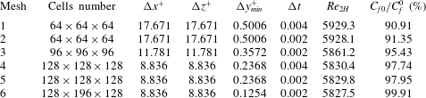
-direction (Moin & Kim Reference Moin and Kim1982; Abe, Kawamura & Matsuo Reference Abe, Kawamura and Matsuo2001). Results summarized in table 1 demonstrate that
 $C_{f0}/C_{f}^{0}\rightarrow 1$
as the grid is refined, as expected. It can be concluded that the grid
 $128^{3}$
as well as the time step 0.002 provide sufficient accuracy. The reader may note that
 $Re_{2H}$
is not imposed but has been computed after the statistically convergent state has been reached.
Mesh convergence study for the DNS method.

4.1.2 Detached eddy simulation
The detached eddy simulation (DES) model is a hybrid technique originally developed for turbulent flows with massive separation. It was first introduced by Spalart, Jou & Allmaras (Reference Spalart, Jou and Allmaras1997) as a modification of the Spalart–Allmaras (S–A) model (Spalart & Allmaras Reference Spalart and Allmaras1992). The S–A model is a one-equation model for the eddy viscosity
 ${\it\nu}_{T}$
dependent on the distance to the closest wall
 $d_{w}$
;
 $d_{w}$
from the original S–A model has been replaced with
 $\tilde{d}$
defined as
 $$\begin{eqnarray}\displaystyle \tilde{d}=\min (d_{w},C_{DES}{\it\Delta}), & & \displaystyle\end{eqnarray}$$
where
 $C_{DES}$
is a parameter that controls the switch point between the near wall and far fields and
 ${\it\Delta}$
represents the largest grid spacing in all three directions, i.e.
 ${\it\Delta}=\max ({\rm\Delta}x,{\rm\Delta}y,{\rm\Delta}z)$
, resulting in the DES model. In the near-wall regions (
 $d_{w}<C_{DES}{\it\Delta}$
), the DES model acts as the Reynolds average Navier–Stokes (RANS) model. Conversely, it behaves as the large eddy simulation (LES) model when
 $d_{w}>C_{DES}{\it\Delta}$
. Overall, the grid resolution of DES is not as demanding as the pure LES approach, thereby reducing the cost of computations. The DES model has been used in this work with the constant
 $C_{DES}$
taken as 0.65 (see Shur et al.
Reference Shur, Spalart, Strelets and Travin1999). It is a proper choice which ensures a narrow transition region between RANS and LES, resulting in accurate results from DES (Keating & Piomelli Reference Keating and Piomelli2006). The convergence has been enhanced using modifications to the S–A model as described by Tu et al. (Reference Tu, Aliabadi, Patel and Watts2009). The time step size and the spatial grid used in the DES algorithm are the same in the DNS.
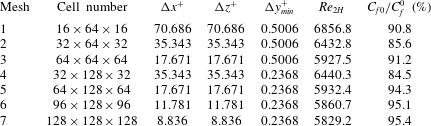
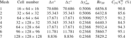
A mesh resolution study for DES has been carried out in the same manner as for DNS. The results displayed in table 2 demonstrate that the grid
 $64\times 128\times 64$
provides sufficient accuracy. While the grid
 $128^{3}$
provides greater accuracy, the potential gains are outweighed by the computational cost. As the primary objective of this study is to determine variations of the discharge as a function of the wall geometry, it has been concluded that the grid
 $64\times 128\times 64$
provides a good compromise between the cost and the desired accuracy.
Mesh convergence study for the DES method.
The size of the computational box may affect the overall accuracy if this box is too small and thus unable to capture large coherent flow structures. Results of testing displayed in table 3 for three different computational boxes demonstrate that variations of (
 $C_{f0}/C_{f}^{0}$
) are within 0.5 % and, thus, the smallest box is large enough to accurately reproduce the flow physics.
Next, the domain independence study is conducted to obtain the effects of spatial dimensions on capturing the relevant flow structures which may impact the calculated friction. The results of three different domain sizes are listed in table 3. The fact that the variations of the friction ratio (
 $C_{f0}/C_{f}^{0}$
) are in the range of 0.5 % demonstrates the present results are fairly independent of the domain size.
Study of the effects of the size of the computational box for the DES method.

4.1.3 The mean velocity profile, the turbulent kinetic energy and the Reynolds stress
The mean velocity profiles, the turbulent kinetic energy and the Reynolds stress determined using both DNS with grid
 $128^{3}$
and DES with grid
 $64\times 128\times 64$
and a computational box (
 $2{\rm\pi}\times 2\times 2{\rm\pi}$
) as displayed in figure 5 demonstrate the consistency between DNS and DES. The mean velocity profiles match fairly well with those obtained by Moser et al. (Reference Moser, Kim and Mansour1999), though the velocities given by DNS and DES are slightly higher in the log-law region, leading to an underestimation of the drag coefficient (approximately 6 % for DES and 2 % for DNS). Figure 6 displays the turbulent kinetic energy components (
 $\langle u^{\prime 2}\rangle$
,
 $\langle v^{\prime 2}\rangle$
and
 $\langle w^{\prime 2}\rangle$
) and the Reynolds stress (
 $\langle u^{\prime }v^{\prime }\rangle$
). Results produced using DES and DNS agree fairly well with those given by Moser et al. (Reference Moser, Kim and Mansour1999) with the peak value of
 $\langle u^{\prime 2}\rangle$
given by DES and DNS being slightly higher than that of Moser et al. (Reference Moser, Kim and Mansour1999) while the position of the peak at
 $y^{+}=15$
is captured correctly.
Distribution of the mean velocity
 $U$
in a smooth channel for
 $Re_{{\it\tau}}=180$
.

Distributions of the turbulent kinetic energy components (a) and the Reynolds stress
 $\langle u^{\prime }v^{\prime }\rangle$
(b) for
 $Re_{{\it\tau}}=180$
.

Sinusoidal, triangular and trapezoidal grooves used in the analysis.

One can conclude that the DES and DNS results produced during code validation agree fairly well with the DNS results obtained by Moser et al. (Reference Moser, Kim and Mansour1999); the minor differences are likely due to the lower spatial resolution of the finite-volume method (FVM). The FVM-based DNS/DES with the selected resolution may not provide the same level of accuracy as the spectral DNS method due to the possibly unresolved small-scale motions, which may lead to underestimation of the turbulent kinetic energy and the Reynolds stress herein. However, the bulk flow manipulation inside the corrugated channel is directly influenced by the cross-section shape (as opposed to the near-wall effect); the small-scale motions near the wall and its effects are not the main focus of the current study. In addition, the key features and trend of the turbulent flow like the drag coefficient, the velocity profile, the turbulent kinetic energy and the Reynolds stress, can be well reproduced using the finite-volume-based DES method and thus this method has been used in the study of corrugated channels.
4.2 Validation of DES for turbulent flows in corrugated channels
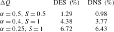
Tests carried out for flows in smooth channels demonstrated that DES provides accuracy similar to DNS. It remains to be demonstrated that both methods provide a similar accuracy for grooved channels. Results presented in table 4 show a discharge difference of less than 0.5 % between the methods which justifies the use of the more computationally efficient DES method.
The difference of the discharge determined using the DES and DNS methods for
 $Re_{{\it\tau}}=180$
.

4.3 Reduced geometry model for turbulent channel flows
It has been demonstrated that sinusoidal grooves play the role of the reduced geometry model for laminar flows (Mohammadi & Floryan Reference Mohammadi and Floryan2013b ; Moradi & Floryan Reference Moradi and Floryan2013). We shall demonstrate that such grooves also represent the reduced geometry model in turbulent flows. We shall use triangular and trapezoidal grooves illustrated in figure 7 for this demonstration.
Table 5 displays results for groove wavenumber
 ${\it\alpha}=0.25$
and amplitude
 $S=1$
. It can be seen that the difference in the discharge obtained for the actual groove and for the same groove with its shape approximated by the leading Fourier mode from its Fourier expansion is less than 1 %. This demonstrates that the concept of the reduced geometry model can be used in the analysis of turbulent flows and thus further discussion is focused on sinusoidal grooves only. It shall be noted that although there are indications that the reduced geometry model works for turbulent flows, the assessment of uncertainties herein is approximate.
Comparison of the discharge through the grooved channel with
 ${\it\alpha}=0.25$
and
 $S=1$
determined using the actual groove geometry as well as its approximation in the form of a leading Fourier mode from its Fourier expansion for
 $Re_{{\it\tau}}=180$
.

4.4 Analysis of flows in channels with sinusoidal grooves
We shall now discuss the characteristics of turbulent flows in channels with sinusoidal grooves. The channel geometry is described by (3.6) and the computations have been carried out for
 $Re_{{\it\tau}}=180$
(
 $Re_{2H}\approx 6000$
) using
 $64\times 128\times 64$
mesh and
 ${\rm\Delta}t=0.002$
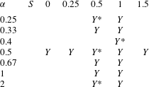
. DNS has been used only for a few geometries (see table 6) due to high computational cost for channels with long-wavelength grooves.
List of the groove configurations studied. ‘
 $Y$
’ identifies configurations studied using only DES and ‘
 $Y$
*’ identifies configurations studied using both DNS and DES.

Figure 8 displays variations of the difference between the discharges through the corrugated and smooth channels generated by the same pressure gradient. The existence of a critical groove wavenumber
 ${\it\alpha}_{c}$
, which separates the discharge-increasing grooves from the discharge-reducing grooves, is clearly documented. The critical wavenumber is estimated to be
 ${\it\alpha}_{c}\approx 1$
for
 $S=0.5$
and approximately
 ${\it\alpha}_{c}\approx 0.8$
for
 $S=1$
. These values are similar to the
 ${\it\alpha}_{c}$
found in laminar flows (
 ${\it\alpha}_{c}=1.2$
). An increase of the groove amplitude
 $S$
decreases the discharge when
 ${\it\alpha}>{\it\alpha}_{c}$
and, conversely, increases the discharge when
 ${\it\alpha}<{\it\alpha}_{c}$
. A decrease of
 ${\it\alpha}$
increases the discharge but this increase rapidly approaches an asymptotic limit where any further decrease of
 ${\it\alpha}$
brings in negligible contributions. The highest increase of the discharge at
 $S=0.5$
is approximately 2 %–3 % , and it is approximately 9 % at
 $S=1$
. The maximization of the discharge requires the use of the minimum possible groove wavenumber
 ${\it\alpha}$
as well as the largest possible groove amplitude
 $S$
.
Variations of the discharge correction
 ${\rm\Delta}Q$
as a function of the groove wavenumber
 ${\it\alpha}$
, (a) and as a function of the groove amplitude
 $S$
(b) for channel with geometry described by (3.6) for
 $Re_{{\it\tau}}=180$
. Symbols identify computed cases while lines result from interpolation.

Distributions of the mean velocity component
 $U$
in the
 $y$
–
 $z$
plane of channel with geometry described by (3.6) with
 ${\it\alpha}=0.25,S=0.5$
(a),
 ${\it\alpha}=0.25,S=1$
(b),
 ${\it\alpha}=0.5,S=0.5$
(c),
 ${\it\alpha}=0.5,S=1$
(d),
 ${\it\alpha}=2,S=0.5$
(e) and
 ${\it\alpha}=2,S=1$
(f) for
 $Re_{{\it\tau}}=180$
.

Distribution of the mean velocity component
 $U$
in the
 $y$
–
 $z$
plane of a smooth channel and averaged only in the streamwise direction for
 $Re_{{\it\tau}}=180$
.

Figure 9 displays distributions of
 $U$
in spanwise cross-sections. The fluid either accelerates or retains its velocity in the wide segment of the channel and slows down in the narrow segment. When
 ${\it\alpha}<{\it\alpha}_{c}$
(figure 9
a–d), the difference between the maximum velocity in the widest and narrowest sections of the channel is larger than the similar difference for channels with
 ${\it\alpha}>{\it\alpha}_{c}$
(figure 9
e,f). The velocity maximum at the widest section of the channel for
 ${\it\alpha}<{\it\alpha}_{c}$
is higher than the maximum velocity in the smooth channel (
 $U\approx 19$
; figure 10) and this results in an increase in the discharge. The discharge increase is most pronounced for conditions used in figure 9(b) where the maximum velocity reaches value of
 $U\approx 24$
. When
 ${\it\alpha}>{\it\alpha}_{c}$
(figure 9
e,f), the maximum velocity in the widest portion of the channel is
 $U\approx$
18–19, which is similar to that found in the smooth channel and, since velocity decreases in the narrow section, there is an overall reduction in the discharge.
The effect of the grooves on the flow discharge is qualitatively similar to that found in laminar flows. The presence of the grooves results in the rearrangement of the bulk motion which leads to the formation of stream tubes of high velocity fluid centred at the widest channel opening, as illustrated in figure 9. The stream tubes exist for
 ${\it\alpha}<{\it\alpha}_{c}$
as well as for
 ${\it\alpha}>{\it\alpha}_{c}$
but play a different role in each case. The difference is illustrated in figure 11 which displays distributions of
 $U$
in the
 $y$
–
 $z$
plane. It can be seen that the flow is redirected towards the wider channel section when
 ${\it\alpha}<{\it\alpha}_{c}$
with a minor velocity decrease in the narrow section; it is the increase of the channel opening in the widest section which dominates the discharge. When
 ${\it\alpha}>{\it\alpha}_{c}$
, the flow is ‘choked’ in the narrowest section while it retains the original velocity in the widest section; it is the decrease of the channel opening in the narrowest section which dominates the discharge.
The lack of smoothness of velocity contours in figure 9 is due to the turbulent structures whose effect has not been completely eliminated by the averaging procedure. The scale of these structures depends on the wall length scale
 $l^{\ast }$
but is almost independent of the groove wavelength (compare figures 9 and 11).
Distributions of the mean velocity
 $U$
in the
 $y$
–
 $z$
plane for channel geometry described by (3.6) with
 ${\it\alpha}=0.5$
,
 $S=0.5$
(a) and with
 ${\it\alpha}=2$
,
 $S=0.5$
(b) for
 $Re_{{\it\tau}}=180$
.

We shall now discuss changes in the velocity profiles resulting from the introduction of the grooves. The velocity profile for the smooth wall consists of three layers, i.e.
-
(i) viscous sub-layer, (
 $y^{+}<7$
, where
$U=y^{+}$
),
-
(ii) buffer layer, (
$7<y^{+}<30$
) and -
(iii) inertial sub-layer, (
$y^{+}>30$
,
$U=(1/{\it\kappa})\ln y^{+}+C$
, with
${\it\kappa}\approx 0.38$
–0.41 and
$C\approx 5$
–5.5).


The velocity profiles in the corrugated channel for conditions leading to an increase in discharge (
 ${\it\alpha}=0.5$
,
 $S=0.5$
) and a reduction in discharge (
 ${\it\alpha}=2$
and
 $S=0.5$
) are displayed in figure 12 for three locations in the spanwise direction; plane 1 corresponds to the narrowest channel opening, plane 2 corresponds to the mean channel opening (the neutral section) and plane 3 corresponds to the widest channel opening (see figure 12
a). In all cases, the velocity profiles consist of the linear region, the buffer region and the log-law region, similarly as in the smooth channel.
Variations of the mean velocity
 $U$
as a function of
 $y^{+}$
at three spanwise locations identified in (a) for channel geometry described by (3.6) with
 ${\it\alpha}=0.5$
,
 $S=0.5$
(b,d) and with
 ${\it\alpha}=2$
,
 $S=0.5$
(c,e) for
 $Re_{{\it\tau}}=180$
. The origins of the
 $y$
-coordinates at different planes have been overlapped to simplify comparisons.

In the case of the discharge increase (
 ${\it\alpha}=0.5$
,
 $S=0.5$
), the velocity profile in plane 2 is nearly identical to the velocity in the smooth channel. The velocity in plane 1 (the narrowest opening) is smaller than in the smooth channel resulting in smaller
 $\partial U/\partial y^{+}$
at the wall (see figure 12
d). The velocity in plane 3 (the widest opening) is higher than in the smooth channel with the difference increasing as
 $y^{+}$
increases. In the case of the discharge reduction (
 ${\it\alpha}=2$
,
 $S=0.5$
),
 $U$
in plane 2 is smaller than in the smooth channel resulting in smaller
 $\partial U/\partial y^{+}$
. Values of
 $U$
in the remaining planes are slightly smaller than in the smooth channel for
 $y^{+}<20$
(see figure 12
e); as
 $y^{+}$
increases, the velocity in plane 3 (the widest channel opening) becomes similar to that in the smooth channel while the velocity in plane 1 (the narrowest channel opening) becomes smaller than in the smooth channel.
4.5 Skin friction
An understanding of the skin friction is essential as it describes the mechanism responsible for drag creation. The total drag is unaltered by the addition of the grooves as the mean pressure gradient is kept unchanged. Thus, the integration of the shear stress over the wetted area must produce the same result regardless of the groove shape while the discharge may vary significantly depending on the groove shape. The reader may note that the addition of the grooves increases the wetted area and thus an increase in the discharge may occur only if the shear decreases sufficiently in order to balance the larger wetted area. Variations of the normalized skin friction
 $Sm/Sm_{0}$
are presented in figure 13(b,c). Here the projected area represents the projection of the actual surface onto the plane
 $y=\text{const.}$
and it is the same as the relevant area of the smooth channel.
Data displayed in figure 13(a) provide a comparison between the distribution of the local shear stress (
 $Sm(0,z)$
on a slice at
 $x=0$
) and its streamwise average (
 $Sm(z)$
). Spanwise fluctuations of the local shear stress at a specific
 $x$
-location are reduced when the streamwise averaging is used (see figure 13
a). We shall use the streamwise averaged data in the following discussion.
The normalized shear acting on the corrugated surface in a channel with geometry described by (3.6) for
 $Re_{{\it\tau}}=180$
. Comparison of the streamwise averaged and non-averaged data is given in (a). The spanwise distributions for
 $S=0.5$
and selective
 ${\it\alpha}$
are given in (b), and for
 ${\it\alpha}=0.5$
and selective
 $S$
are given in (c).

Figure 13(b) depicts the effect of the groove wavenumber on the skin friction. When
 ${\it\alpha}<{\it\alpha}_{c}$
in the discharge-increase case,
 $Sm/Sm_{0}>1$
in the wide section and
 $Sm/Sm_{0}<1$
in the narrow section. Reduction of
 ${\it\alpha}$
produces larger
 $Sm/Sm_{0}$
in the wide section and smaller
 $Sm/Sm_{0}$
in the narrow section (compare results for
 ${\it\alpha}=0.25$
and 0.5). When
 ${\it\alpha}>{\it\alpha}_{c}$
in the discharge reduction case,
 $Sm/Sm_{0}\approx 1$
in both the wide and narrow sections. The physical distance between these two sections are small, which results in similar momentum transport characteristics and leads to a more uniform skin friction. The reader may note that the shear variations in the streamwise direction must average out as the mean stress
 $Sm/Sm_{0}$
is always 1 (the total drag remains the same).
Figure 13(c) illustrates the effects of the groove amplitude for
 ${\it\alpha}=0.5<{\it\alpha}_{c}$
.
 $Sm/Sm_{0}$
in the wide section increases with increasing
 $S$
, but decreases in the narrow section. This is due to the fact that the larger groove amplitude accentuates the velocity difference between the wide and narrow sections of the channel.
4.6 The turbulent flow quantities
It has been documented so far that the presence of the grooves leads to the rearrangement of the mean velocity profile which results in an increase in the discharge. We shall now discuss how the turbulence characteristics change in response to the grooves.
The components of the turbulent kinetic energy (TKE)
 $k=(\langle u^{\prime 2}\rangle +\langle v^{\prime 2}\rangle +\langle w^{\prime 2}\rangle )/2$
and the dominant component of Reynolds shear stress (
 $\langle u^{\prime }v^{\prime }\rangle$
) for grooves with
 ${\it\alpha}=0.5$
,
 $S=0.5$
and
 ${\it\alpha}=2$
,
 $S=0.5$
, determined using DNS, are displayed in figures 14 and 15 respectively. Our intention is to show and highlight the behaviour of the dominant component of Reynolds stress
 $\langle u^{\prime }v^{\prime }\rangle$
at the three planes in comparison to the smooth channel at plane 2. The remaining components of (lower magnitude) Reynolds stress
 $\langle u^{\prime }w^{\prime }\rangle$
and
 $\langle v^{\prime }w^{\prime }\rangle$
are plotted in the
 $y$
–
 $z$
plane for comparison of the different cases as shown in figure 16. It should be noted that
 $\langle u^{\prime }w^{\prime }\rangle$
and
 $\langle v^{\prime }w^{\prime }\rangle$
are zero for a smooth channel.
Distributions of the TKE in the corrugated and smooth channels for
 $Re_{{\it\tau}}=180$
. (a) and (c) display
 $\langle u^{\prime 2}\rangle$
,
 $\langle v^{\prime 2}\rangle$
and
 $\langle w^{\prime 2}\rangle$
for grooves described by (3.6) with
 ${\it\alpha}=0.5$
,
 $S=0.5$
while (b) and (d) display the same quantities for
 ${\it\alpha}=2$
,
 $S=0.5$
. The total kinetic energy total
 $k$
is displayed in (e) and (f) for
 ${\it\alpha}=0.5$
,
 $S=0.5$
and
 ${\it\alpha}=2$
,
 $S=0.5$
, respectively.

Figure 14 displays data for the narrowest channel opening (plane 1 in figure 12
a), the mean opening (plane 2) and the widest opening (plane 3). Note that the
 $y$
-axis used herein based on the same
 $y$
origin location is different from the
 $y^{+}$
starting from wall used in figure 12. The qualitative characteristics of variations of all quantities in all planes are similar to those found in the smooth channel, i.e. they rapidly increase in the viscous sub-layer (
 $y^{+}<15$
), reach peak values in the buffer layer (
 $y^{+}\approx 15$
) and decrease in the inertial sub-layer (
 $y^{+}>15$
).
Results displayed in figure 14(a,c,e) demonstrate that all quantities in plane 2 for
 ${\it\alpha}=0.5<{\it\alpha}_{c}$
(discharge-increase case) are nearly the same as in the smooth channel. The peak values in plane 1 (the narrowest section) are lower than in the smooth channel, which is possibly due to the maximum velocity being smaller than in the smooth channel. The peak values in plane 3 (the widest opening) are higher than those in the smooth channel due to the maximum velocity being larger than in the smooth channel. In the discharge-reduction case (
 ${\it\alpha}=2>{\it\alpha}_{c}$
) the situation becomes more complex (see figure 14
b,d,f). In plane 2 (the neutral section),
 $\langle u^{\prime 2}\rangle$
is slightly smaller than in the smooth channel in both the viscous sub-layer and the buffer layer, but is slightly larger in the inertial sub-layer. One may conclude that the distribution of
 $\langle u^{\prime 2}\rangle$
in this plane shifts towards the centre of the channel when compared to the smooth channel. In plane 1, the peak of
 $\langle u^{\prime 2}\rangle$
is smaller than in the smooth channel, and similar to plane 1 for the discharge-increase case (
 ${\it\alpha}=0.5$
). The peak of
 $\langle u^{\prime 2}\rangle$
in plane 3 is similar to the smooth channel and, thus, smaller than that in the discharge-increase case. Both
 $\langle v^{\prime 2}\rangle$
and
 $\langle w^{\prime 2}\rangle$
in all three planes are approximately similar to the smooth channel, which is possibly due to the weak rearrangement of the bulk motion. One can observe that
 $\langle u^{\prime 2}\rangle$
represents the largest component of TKE and, thus, it dictates the properties of TKE.
Distributions of
 $\langle u^{\prime }v^{\prime }\rangle$
in the corrugated channel with shape described by (3.6) and in the smooth channel for
 $Re_{{\it\tau}}=180$
. Data displayed in (a) correspond to
 ${\it\alpha}=0.5$
,
 $S=0.5$
(discharge-increase case); data displayed in (b) correspond to
 ${\it\alpha}=2$
,
 $S=0.5$
(discharge-reduction case).

Figure 15 displays distributions of
 $\langle u^{\prime }v^{\prime }\rangle$
. In the discharge-increase case (
 ${\it\alpha}=0.5$
), its magnitude in plane 2 (the neutral section) is slightly smaller than in the smooth channel, it is smaller in plane 1 (the narrowest section) and it is larger in plane 3 (the widest section). In the discharge-reduction case (
 ${\it\alpha}=2$
), its magnitude in plane 2 is smaller within the viscous sub-layer and in the buffer layer but slightly larger within the inertial sub-layer. In plane 1 (the narrowest section), the peak values are lower than in the smooth channel. In plane 3 (the widest section), the peak value is similar to that in plane 1.
It can be concluded that in the discharge-increase case (
 ${\it\alpha}<{\it\alpha}_{c}$
), TKE and Reynolds shear stress
 $\langle u^{\prime }v^{\prime }\rangle$
in the wide section are higher and in the narrow section are smaller than in the smooth channel. In the discharge-reduction case (
 ${\it\alpha}>{\it\alpha}_{c}$
), TKE and Reynolds shear stress
 $\langle u^{\prime }v^{\prime }\rangle$
are smaller in the narrow section and similar to the smooth channel in the wide section. The distributions of TKE and Reynolds shear stress
 $\langle u^{\prime }v^{\prime }\rangle$
shift towards plane 2 (neutral plane) for the discharge-reduction case (
 ${\it\alpha}>{\it\alpha}_{c}$
). This may be due to the smaller physical distance between the wide and narrow sections and, hence, larger spanwise velocity gradients which, in turn, produce more intense turbulent fluctuations near the neutral plane.
Distributions of
 $\langle u^{\prime }w^{\prime }\rangle$
and
 $\langle v^{\prime }w^{\prime }\rangle$
in the corrugated channel with shape described by (3.6) for
 $Re_{{\it\tau}}=180$
. Data displayed in (a) and (c) correspond to
 ${\it\alpha}=0.5$
,
 $S=0.5$
(discharge-increase case); data displayed in (b) and (d) correspond to
 ${\it\alpha}=2$
,
 $S=0.5$
(discharge-reduction case).

In order to show the complexity of distributions of Reynolds shear stresses
 $\langle u^{\prime }w^{\prime }\rangle$
and
 $\langle v^{\prime }w^{\prime }\rangle$
, these quantities are presented in the form of contour plots in the
 $y$
–
 $z$
plane (see figure 16) rather than as 1-D cuts along the
 $y$
-axis in planes 1, 2, 3 as such cuts do not exhibit any distinctive features. The theoretical arguments suggest that
 $\langle u^{\prime }w^{\prime }\rangle$
and
 $\langle v^{\prime }w^{\prime }\rangle$
should be zero in the smooth channel and very close to zero in numerical simulation of such a flow with non-zero values arising from numerical round-off errors. One may interpret
 $\langle u^{\prime }w^{\prime }\rangle$
and
 $\langle v^{\prime }w^{\prime }\rangle$
as representing the interactions between the fast fluid in the wide section of the channel and the slow fluid in the narrow section. As a result, the highest magnitudes of
 $\langle u^{\prime }w^{\prime }\rangle$
and
 $\langle v^{\prime }w^{\prime }\rangle$
are located around plane 2 (neutral plane) where the strongest spanwise interactions occur. Such interactions for the discharge-reduction case (
 ${\it\alpha}=2$
) are more intense than for the discharge-increase case (
 ${\it\alpha}=0.5$
) because of the reduction in the physical distance between the wide and narrow sections of the channel.
The volume-averaged (a) TKE
 $[k]$
; (b)
 $[|\langle u^{\prime }v^{\prime }\rangle |]$
; (c)
 $[|\langle u^{\prime }w^{\prime }\rangle |]$
and
 $[|\langle v^{\prime }w^{\prime }\rangle |]$
for
 $Re_{{\it\tau}}=180$
.

The effects of the groove wavenumber can be clarified by looking at the volume-averaged values of TKE
 $[k]$
and the absolute values of the Reynolds shear stresses
 $[|\langle u^{\prime }v^{\prime }\rangle |]$
,
 $[|\langle u^{\prime }w^{\prime }\rangle |]$
,
 $[|\langle v^{\prime }w^{\prime }\rangle |]$
, which are displayed in figure 17 for
 ${\it\alpha}=0.5$
, 1, 2 with
 $S=0.5$
. The volume-averaging operator
 $[\,]$
is defined as
 $$\begin{eqnarray}\displaystyle [\natural ]=\frac{\displaystyle \int _{{\rm\Omega}}\natural \,\text{d}V}{\displaystyle \int _{{\rm\Omega}}\,\text{d}V}. & & \displaystyle\end{eqnarray}$$
The reader may note that
 $[|\langle u^{\prime }w^{\prime }\rangle |]$
and
 $[|\langle v^{\prime }w^{\prime }\rangle |]$
are both zero in the smooth channel. The volume-averaged TKE
 $[k]$
for the corrugated channel is slightly higher (approximately 6 %) than that for the smooth channel,
 $[|\langle u^{\prime }w^{\prime }\rangle |]$
and
 $[|\langle v^{\prime }w^{\prime }\rangle |]$
are also higher than in the smooth channel and increase with increasing wavenumber.
 $[|\langle u^{\prime }v^{\prime }\rangle |]$
in the corrugated channel is slightly higher than in the smooth channel for the discharge increase case (
 ${\it\alpha}=0.5$
) and is slightly lower for the discharge reduction case (
 ${\it\alpha}=2$
).
The above discussion shows that corrugations can rearrange the distribution of TKE and the Reynolds stress, but are unable to significantly reduce the global turbulence intensity.
The distributions of the TKE and the Reynolds stress discussed in the previous section imply that there is less turbulent activity in the narrow portion of the corrugated channel and stronger turbulent activity in the wide portion in the discharge-increase case (
 ${\it\alpha}<{\it\alpha}_{c}$
). We shall now look at the turbulence structures in order to better understand the character of the flow in each case.
Ensemble time-averaging Reynolds shear stress
 $\langle u^{\prime }v^{\prime }\rangle$
with quadrant detection (Q2 for ejection events (a,b) and Q4 for sweep events (c,d)) in a corrugated channel described by (3.6) with
 ${\it\alpha}=0.5$
,
 $S=0.5$
(a,c) and with
 ${\it\alpha}=2$
,
 $S=0.5$
(b,d) for
 $Re_{{\it\tau}}=180$
.

In figure 18, the ensemble time-averaging Reynolds shear stress
 $\langle u^{\prime }v^{\prime }\rangle$
is presented with quadrant detection for ejection events (Q2) and for sweep events (Q4). Figure 18(a,c) demonstrates that in the discharge increase case (
 ${\it\alpha}<{\it\alpha}_{c}$
) most of the near-wall turbulent motions (ejection and sweep) tend to gather in the wide section of the channel. This may be due to the fact that the maximum velocity in the wide portion is much larger than that in the narrow portion. An increase in the ejection/sweep suggests the occurrence of more intense bursting phenomena, stronger turbulent motions and higher TKE, and this is consistent with the findings presented in figures 14(a,e) and 15(a).
Results presented in figure 18(b) demonstrate that in the discharge-reduction case (
 ${\it\alpha}>{\it\alpha}_{c}$
) the ejection motions tend to occur in the neutral section, which may be associated with the strong velocity gradient between the wide and narrow sections with a short physical distance between them. Figure 18(d) shows that there is no obvious tendency of gathering of sweep motions either in the wide or in the narrow portions of the channel, which is balanced by the momentum transport between the wide and narrow sections. This observation is consistent with the results displayed in figures 14(b,f) and 15(b). It is very interesting to observe that the ejection and sweep behave differently in the discharge-increase and discharge-reduction cases.
In summary, the analysis of TKE, the Reynolds stress and the turbulent structures shows that the turbulence intensity in the narrow portion of the channel is suppressed. When the groove amplitude is high (
 $S\rightarrow 2$
), the narrow section shrinks to a triangular corner and the flow is expected to relaminarize (Eckert & Irvine Jr Reference Eckert and Irvine1956). These results led to the creation of the concept of riblets for turbulent drag reduction (Walsh & Weinstein Reference Walsh and Weinstein1978; Walsh & Lindeman Reference Walsh and Lindeman1984).
4.7 Analysis of flow changes caused by the small-wavenumber grooves
Interactions between the wide and narrow sections of the channel weaken when
 ${\it\alpha}\rightarrow 0$
and thus each section might behave as a smooth channel but with different heights and the same pressure gradient.
First, we shall demonstrate that the local flow properties become very similar when expressed in terms of the local scales. The local half-channel height
 ${\it\delta}^{\ast }$
, the local friction velocity
 $u_{{\it\tau}e}^{\ast }$
, the local friction Reynolds number
 $Re_{{\it\tau}e}$
and the local wall length
 $l_{e}^{\ast }$
are defined as
 $$\begin{eqnarray}\displaystyle & \displaystyle {\it\delta}^{\ast }=H^{\ast }\left(1+\frac{S}{2}\sin {\it\alpha}z\right), & \displaystyle\end{eqnarray}$$
 $$\begin{eqnarray}\displaystyle & \displaystyle u_{{\it\tau}e}^{\ast }=\sqrt{\frac{{\it\beta}^{\ast }{\it\delta}^{\ast }}{{\it\rho}^{\ast }}}, & \displaystyle\end{eqnarray}$$
 $$\begin{eqnarray}\displaystyle & \displaystyle Re_{{\it\tau}e}=\frac{u_{{\it\tau}e}^{\ast }{\it\delta}^{\ast }}{{\it\nu}^{\ast }}=Re_{{\it\tau}}\left(1+\frac{S}{2}\sin {\it\alpha}z\right)^{3/2}, & \displaystyle\end{eqnarray}$$
 $$\begin{eqnarray}\displaystyle & \displaystyle l_{e}^{\ast }=\frac{{\it\nu}^{\ast }}{u_{{\it\tau}e}^{\ast }}, & \displaystyle\end{eqnarray}$$
 $_{e}$
stands for local scalar and the superscript
 $^{\ast }$
stands for dimensional scalar.
It can be shown that the ratio between the local and the average friction velocities, the average streamwise velocity scaled with the local friction velocity denoted as
 $U_{e}$
and the wall distance scaled with the local wall length denoted as
 $y_{e}^{+}$
are of the form
 $$\begin{eqnarray}\displaystyle & \displaystyle \frac{u_{{\it\tau}e}^{\ast }}{u_{{\it\tau}}^{\ast }}=\left(1+\frac{S}{2}\sin {\it\alpha}z\right)^{1/2}, & \displaystyle\end{eqnarray}$$
 $$\begin{eqnarray}\displaystyle & \displaystyle U_{e}=\frac{U^{\ast }}{u_{{\it\tau}e}^{\ast }}=\frac{U}{\displaystyle \left(1+\frac{S}{2}\sin {\it\alpha}z\right)^{1/2}}, & \displaystyle\end{eqnarray}$$
 $$\begin{eqnarray}\displaystyle & \displaystyle y_{e}^{+}=\frac{y^{\ast }}{{\it\nu}^{\ast }/u_{{\it\tau}e}^{\ast }}=y^{+}\left(1+\frac{S}{2}\sin {\it\alpha}z\right)^{1/2}. & \displaystyle\end{eqnarray}$$
Distributions of
 $U$
and
 $U_{e}$
as functions of
 $y^{+}$
and
 $y_{e}^{+}$
are presented in figure 19(a,b), respectively. The velocity distributions in the widest, mean and narrowest sections of the corrugated channel are similar to the smooth channel when the local scales are used (figure 19
b) but different when the original scales are used (figure 19
a). Distributions of the largest component of TKE,
 $\langle u^{\prime 2}\rangle$
, displayed in figure 20 demonstrate that the values for all three planes nearly overlap when scaled using the local scales. This suggests that properties of the flow in different planes can be deduced from properties of the flow in a smooth channel through the use of the proper scaling.
Distributions of the average mean velocity
 $U$
for
 $Re_{{\it\tau}}=180$
as a function of
 $y^{+}$
(a) and the local mean velocity
 $U_{e}$
as a function of
 $y_{e}^{+}$
(b) at the widest, mean and narrowest sections of channel with geometry described by (3.6) with
 ${\it\alpha}=0.25$
and
 $S=0.5$
. Symbols identify velocities in the smooth channels with different mean openings.

Distributions of
 $\langle u^{\prime 2}\rangle$
as functions of
 $y^{+}$
(a) and
 $\langle u_{e}^{\prime 2}\rangle$
as functions of
 $y_{e}^{+}$
(b) for
 $Re_{{\it\tau}}=180$
at the widest, mean and narrowest sections of channel with geometry described by (3.6) with
 ${\it\alpha}=0.25$
and
 $S=0.5$
. Symbols identify velocities in the smooth channels with different mean openings.

Use of (4.3), (4.9b ) and (4.9c ) leads to the local velocity gradient at the wall of the form
 $$\begin{eqnarray}\displaystyle \frac{\partial U}{\partial y}=\frac{\partial U_{e}}{\partial y_{e}^{+}}Re_{{\it\tau}}\left(1+\frac{S}{2}\sin {\it\alpha}z\right). & & \displaystyle\end{eqnarray}$$
As
 $\partial U_{e}/\partial y_{e}^{+}=1$
near the wall,
 $$\begin{eqnarray}\displaystyle \frac{Sm}{Sm_{0}}=1+\frac{S}{2}\sin {\it\alpha}z. & & \displaystyle\end{eqnarray}$$
Distribution of the ratio of wall shear
 $Sm/Sm_{0}$
for
 $S=0.5$
and
 $Re_{{\it\tau}}=180$
.

Figure 21 displays the distribution of
 $Sm/Sm_{0}$
given by (4.11) together with DNS results. When
 ${\it\alpha}$
decreases,
 $Sm/Sm_{0}$
approaches the theoretical estimate. Values computed for
 ${\it\alpha}=0.25$
are already very close to the theoretical estimate, implying that the interactions between fluid flowing in different sections of the corrugated channel at
 ${\it\alpha}=0.25$
are very weak and could be neglected.
The above discussion shows that the velocity distribution in an arbitrary
 $x$
–
 $y$
plane of the corrugated channel is similar to the smooth channel when described using the local friction velocity, the local wall length and local friction Reynolds number. Thus, the local mean velocity scaled using the local effective friction velocity
 $u_{{\it\tau}e}^{\ast }$
can be written as (Pope Reference Pope2000)
 $$\begin{eqnarray}\displaystyle U_{be}=\frac{U_{b}^{\ast }}{u_{{\it\tau}e}^{\ast }}=5.6818\log _{10}Re_{{\it\tau}e}+3.5418, & & \displaystyle\end{eqnarray}$$
where
 $U_{b}^{\ast }$
is the dimensional local bulk velocity, and depends on the local effective friction Reynolds number
 $Re_{{\it\tau}e}$
. The local mean velocity scaled using the friction velocity
 $u_{{\it\tau}}^{\ast }$
can be written as
 $$\begin{eqnarray}\displaystyle U_{b}=\left[5.6818\log _{10}Re_{{\it\tau}}+8.5227\log _{10}\left(1+\frac{S}{2}\sin {\it\alpha}z\right)+3.5418\right]\left(1+\frac{S}{2}\sin {\it\alpha}z\right)^{1/2}. & & \displaystyle \nonumber\\ \displaystyle & & \displaystyle\end{eqnarray}$$
Integration of the mean velocity in the spanwise direction
 $z$
leads to the discharge
 $$\begin{eqnarray}\displaystyle Q|_{{\it\alpha}\rightarrow 0} & = & \displaystyle \frac{1}{2{\rm\pi}/{\it\alpha}}\int _{0}^{2{\rm\pi}/{\it\alpha}}2{\it\delta}U_{b}\,\text{d}z\nonumber\\ \displaystyle & = & \displaystyle \frac{(5.6818\log _{10}Re_{{\it\tau}}+3.5418)}{{\rm\pi}}\int _{0}^{2{\rm\pi}}\left[1+\frac{8.5227\log _{10}\left(1+\displaystyle \frac{S}{2}\sin {\it\xi}\right)}{[5.6818\log _{10}Re_{{\it\tau}}+3.5418]}\right]\nonumber\\ \displaystyle & & \displaystyle \times \,\left(1+\frac{S}{2}\sin {\it\xi}\right)^{3/2}\text{d}{\it\xi},\end{eqnarray}$$
where
 $2{\it\delta}$
is the local channel opening at the location
 $z$
.
The discharge for a smooth channel has the form
 $$\begin{eqnarray}\displaystyle Q_{0}|_{{\it\alpha}\rightarrow 0}=Q|_{{\it\alpha}\rightarrow 0}|_{S=0}=2(5.6818\log _{10}Re_{{\it\tau}}+3.5418). & & \displaystyle\end{eqnarray}$$
The ratio of discharges in the corrugated and smooth channels at the same friction Reynolds number (i.e. the same pressure gradient) is
 $$\begin{eqnarray}\displaystyle \left.\frac{Q}{Q_{0}}\right|_{{\it\alpha}\rightarrow 0}=\frac{1}{2{\rm\pi}}\int _{0}^{2{\rm\pi}}\left[1+\frac{8.5227\log _{10}\left(1+\displaystyle \frac{S}{2}\sin {\it\xi}\right)}{[5.6818\log _{10}Re_{{\it\tau}}+3.5418]}\right]\left(1+\frac{S}{2}\sin {\it\xi}\right)^{3/2}\,\text{d}{\it\xi}, & & \displaystyle\end{eqnarray}$$
and gives the discharge difference of the form
 $$\begin{eqnarray}\displaystyle {\rm\Delta}Q|_{{\it\alpha}\rightarrow 0}(S)=\left.\frac{Q}{Q_{0}}\right|_{{\it\alpha}\rightarrow 0}-1. & & \displaystyle\end{eqnarray}$$
The above predictions are compared with the DNS results for a channel with
 $S=0.5$
and
 $S=1$
at
 $Re_{{\it\tau}}=180$
. Equation (4.17) gives
 ${\rm\Delta}Q|_{{\it\alpha}\rightarrow 0}=1.88\,\%$
and
 ${\rm\Delta}Q|_{{\it\alpha}\rightarrow 0}=7.57\,\%$
, respectively, while the numerical results displayed in figure 8(a) give 2 % and 10 %, respectively. This suggests that the above estimate provides quite a good approximation of the discharge through the corrugated channel when the corrugation wave number is sufficiently small.
The above analysis can be extended to flow conditions not accessible to numerical simulations. As an example, consider the limit of very high friction Reynolds number. The discharge ratio for the corrugated and smooth channels is of the form
 $$\begin{eqnarray}\displaystyle \lim _{Re_{{\it\tau}}\rightarrow \infty }{\rm\Delta}Q|_{{\it\alpha}\rightarrow 0}=\frac{1}{2{\rm\pi}}\int _{0}^{2{\rm\pi}}\left(1+\frac{S}{2}\sin {\it\xi}\right)^{3/2}\,\text{d}{\it\xi}-1. & & \displaystyle\end{eqnarray}$$
Figure 22 displays predictions of
 ${\rm\Delta}Q$
based on (4.17) for different Reynolds numbers and groove amplitudes for small
 ${\it\alpha}$
. Data for the laminar flow have been added for comparison. The discharge increases with
 $S$
at any
 $Re_{{\it\tau}}$
. There is a significant drop in the discharge increase when the flow changes from the laminar to turbulent form. In the turbulent state, the magnitude of the discharge increase decreases very slowly as
 $Re_{{\it\tau}}$
increases but remains large enough to be of practical interest.
It has been shown in § 3 that the discharge increases linearly with
 $Re_{{\it\tau}}$
in the case of laminar flow. The above analysis suggests that in the case of turbulent flows the discharge increase is nearly independent of
 $Re_{{\it\tau}}$
. The discharge increase is 7.57 % for
 $Re_{{\it\tau}}=$
180 and would be 7.28 % and 7.15 % for
 $Re_{{\it\tau}}=$
395 and 590 which are the other values of
 $Re_{{\it\tau}}$
frequently used in DNS studies. These cases have not been attempted during the present study due to computational cost and, thus, the
 $Re_{{\it\tau}}$
dependence conjectured above remains to be proven.
It can be concluded that the maximization of the discharge is achieved using grooves with decreasing wavenumber and increasing amplitude. The resulting discharge can increase 20 %–30 % above the smooth channel discharge, depending on the Reynolds number. Though this increase is not as high as in laminar flows (150 %), it is still much higher than what can be achieved using other more traditional drag-reducing methods. It can also be concluded that the discharge-increase results from the bulk velocity rearrangement rather than from the suppression of the turbulence intensity.
Variations of the discharge correction
 ${\rm\Delta}Q$
as a function of
 $S$
at different
 $Re_{{\it\tau}}$
for
 ${\it\alpha}\rightarrow 0$
.

4.8 Additional cases with phase shift
The above discussion dealt with the positioning of the grooves at the upper and lower walls in such a manner that the maximum height of the upper grooves was located above the minimum height of the lower grooves, i.e. the diverging–converging configuration. It is of interest to check how the relative positioning of the upper and lower groove systems affects the flow discharge. This positioning is parameterized using the phase shift
 ${\it\varphi}$
, i.e. the channel geometry is described as
 $$\begin{eqnarray}\displaystyle y_{L}=-1-\frac{S}{2}\sin ({\it\alpha}z),\quad y_{U}=1+\frac{S}{2}\sin ({\it\alpha}z+{\it\varphi}). & & \displaystyle\end{eqnarray}$$
Use of
 ${\it\varphi}=0$
produces the converging–diverging channel and
 ${\it\varphi}={\rm\pi}$
results in the sinusoidal channel for
 ${\it\alpha}=0.5$
and
 $S=1$
(see figure 23). Results displayed in figure 24 demonstrate the converging–diverging channel produces the largest discharge increase. Increase of
 ${\it\varphi}$
from 0 to
 ${\rm\pi}$
reduces this increase and can reduce the total discharge below the smooth channel level if
 ${\it\varphi}$
is close enough to
 ${\rm\pi}$
. The deterioration of the system performance is associated with the reduction and eventual elimination of the stream tube with the fast moving fluid forming in the wide section of the channel, as documented in figure 23. The corresponding changes of the skin-friction distribution are documented in figure 25.
Distributions of the streamwise velocity
 $U$
in the
 $y$
–
 $z$
plane at
 $Re_{{\it\tau}}=180$
for
 ${\it\alpha}=0.5$
and
 $S=1$
with different phase shifts. (a)
 ${\it\varphi}=0$
; (b)
 ${\it\varphi}={\rm\pi}/2$
; (c)
 ${\it\varphi}={\rm\pi}$
.

Variations of the discharge correction
 ${\rm\Delta}Q$
as a function of the phase shift
 ${\it\varphi}$
for
 $Re_{{\it\tau}}=180$
.

Distributions of the shear stress in the
 $y$
–
 $z$
plane for
 ${\it\alpha}=0.5$
and
 $S=1$
with different phase shifts
 ${\it\varphi}$
at
 $Re_{{\it\tau}}=180$
.

5 Concluding remarks
An analysis of the laminar and turbulent flows through corrugated channels, with the grooves being parallel to the flow direction, has been carried out. The analysis relied on the theoretical solution in the laminar case and on the DES method in the turbulent case. It has been demonstrated that the use of the grooves results in an increase of the discharge through the grooved channel when compared with a smooth channel operating under the same pressure gradient. It has been shown that the reduced geometry model applies to turbulent flows, i.e. the groove shape can be replaced by the leading Fourier mode from its Fourier representation and the resulting error is acceptable for most applications. It is therefore possible to parameterize the groove effects using just two parameters, i.e. the groove wavenumber and the groove amplitude. Detailed results have been presented for sinusoidal grooves in the range the Reynolds numbers of interest. Changes in the discharge, the mean velocity distribution, the mean shear distribution, the TKE, the Reynolds stress and the turbulence structures have been documented and discussed.
It has been shown that the corrugated channel, subject to the same pressure gradient as the smooth channel, can produce either larger or smaller discharge depending on the groove wavenumber. There exists a critical groove wavenumber
 ${\it\alpha}_{c}\approx 0.8$
–1 separating both types of grooves, with grooves with
 ${\it\alpha}<{\it\alpha}_{c}$
increasing discharge. An increase of the groove amplitude
 $S$
increases the discharge for
 ${\it\alpha}<{\it\alpha}_{c}$
and decreases the discharge for
 ${\it\alpha}>{\it\alpha}_{c}$
. The grooves are less effective in increasing the discharge in turbulent flows when compared with the laminar flows. The discharge increase in the turbulent flow is approximately 10 % when
 ${\it\alpha}=$
0.25 and
 $S=1$
, which is similar to the discharge increase that can be achieved using riblets (7 %–10 %). A maximum discharge can be achieved for
 ${\it\alpha}\rightarrow 0$
and
 $S\rightarrow 2$
.
The discharge increase is achieved by rearranging the bulk velocity distribution in the transverse (
 $y$
–
 $z$
) plane with the largest fluid flux flowing through the widest channel opening. The grooves do not suppress the TKE production and the Reynolds stress. Change of the phase shift between the groove systems at the upper and lower walls affect the bulk flow. The largest discharge increase is achieved for the converging–diverging form of the channel while no discharge increase can be achieved for the wavy form of the channel.