





1. Introduction
In the course of many years of research on normal shock wave internal structure, it has become a benchmark problem for testing new mathematical models of rarefied and non-equilibrium flows (Pham-Van-Diep, Erwin & Muntz Reference Pham-Van-Diep, Erwin and Muntz1991; Ohwada Reference Ohwada1993; Torrilhon & Struchtrup Reference Torrilhon and Struchtrup2004; Kudryavtsev, Shershnev & Ivanov Reference Kudryavtsev, Shershnev and Ivanov2008; Johnson Reference Johnson2013; Timokhin et al. Reference Timokhin, Struchtrup, Kokhanchik and Bondar2016; Velasco & Uribe Reference Velasco and Uribe2019; Shoev, Timokhin & Bondar Reference Shoev, Timokhin and Bondar2020; Jadhav, Gavasane & Agrawal Reference Jadhav, Gavasane and Agrawal2021). It has been caused by the importance of shock-wave phenomena in real-life applications, simplicity of the mathematical formulation and availability of experimental data (Hansen & Hornig Reference Hansen and Hornig1960; Schmidt Reference Schmidt1969; Alsmeyer Reference Alsmeyer1976; Pham-Van-Diep, Erwin & Muntz Reference Pham-Van-Diep, Erwin and Muntz1989; Timokhin et al. Reference Timokhin, Tikhonov, Mursenkova and Znamenskaya2020).
The bimodal Mott-Smith (M-S) solution (Mott-Smith Reference Mott-Smith1951; Tamm Reference Tamm1965) is a classical solution of this fundamental problem. The solution of the Boltzmann equation is based on the approximation of the non-equilibrium molecular velocity distribution in the form of the sum of two Maxwellians with unknown weight coefficients. The Maxwellians correspond to two equilibrium states of the gas on opposite sides of the shock wave. The bimodal character of the distribution function becomes more evident with the increase of shock wave Mach number. It leads to the fact that this analytical solution is more applicable for prediction of the phase density for strong shock waves (e.g. Kogan Reference Kogan1969; Bird Reference Bird1967; Pham-Van-Diep et al. Reference Pham-Van-Diep, Erwin and Muntz1989; Xu & Huang Reference Xu and Huang2010; Timokhin & Rukhmakov Reference Timokhin and Rukhmakov2021). Further investigation of the shock wave structure showed that the M-S solution does not allow reproduction of such non-equilibrium effects as temperature overshoot (e.g. Holway Reference Holway1965b; Erofeev & Friedlander Reference Erofeev and Friedlander2002; Ivanov et al. Reference Ivanov, Kryukov, Timokhin, Bondar, Kokhanchik and Ivanov2012; Timokhin et al. Reference Timokhin, Bondar, Kokhanchik, Ivanov, Ivanov and Kryukov2015). Mott-Smith's original approach was later modified by using different basis functions (Muckenfuss Reference Muckenfuss1962; Holway Reference Holway1965a; Kogan Reference Kogan1969; Solovchuk & Sheu Reference Solovchuk and Sheu2010), or the introduction of the third basis function (Salwen, Grosch & Ziering Reference Salwen, Grosch and Ziering1964). These modifications made the M-S approximation much closer to the Boltzmann equation solution for a wide range of Mach numbers (e.g. Solovchuk & Sheu Reference Solovchuk and Sheu2010, Reference Solovchuk and Sheu2011).
Despite the existing disadvantages of the original M-S solution in the quantitative description of the structure of a one-dimensional (1-D) shock wave, this solution provides excellent qualitative description of the transition of a gas from one equilibrium state to the other across the shock at the level of molecular velocity distributions.
2. Problem formulation and mathematical model
Real supersonic flows are rarely 1-D. Among steady two-dimensional (2-D) flows, there are some examples that retain important features of the 1-D normal shock wave problem. Probably the simplest example is the problem of stationary regular reflection of an oblique shock wave from the plane of symmetry (e.g. Ben-Dor Reference Ben-Dor2007; Xue et al. Reference Xue, Schrijer, van Oudheusden, Wang, Shi and Cheng2020). Such a flow is illustrated by a numerical density flow field as shown in figure 1. The direction of the supersonic flow (region 1) is from left to right. The flow is deflected in the oblique incident shocks (IS) and returns to its original direction passing through the reflected shocks (RS). The angles of incident and reflected oblique shock waves are denoted in figure 1 as  $\alpha$ and
 $\beta$, respectively. It should be noted that the inviscid solution of this problem consists of four zones of a uniform supersonic flow divided by discontinuities (in contrast with two uniform flow regions divided by one discontinuity in the 1-D shock case). This solution can be determined analytically if one knows the incoming flow Mach number and the IS angle
 $\alpha$ (Ben-Dor Reference Ben-Dor2007). Similarly, in the inviscid 1-D normal shock problem the analytical solution consists of two zones of uniform flow divided by one discontinuity and is fully determined by the shock Mach number. In this regard, the regular reflection problem can be considered as an extension of the normal shock structure problem to a more complicated 2-D case. If viscosity and heat conduction are taken into account, the shock waves acquire their internal structure, and in the vicinity of the reflection point (the origin in figure 1) the flow becomes essentially 2-D (Ivanov et al. Reference Ivanov, Ben-Dor, Elperin, Kudryavtsev and Khotyanovsky2002; Khotyanovsky et al. Reference Khotyanovsky, Bondar, Kudryavtsev, Shoev and Ivanov2009; Bondar et al. Reference Bondar, Shoev, Kokhanchik and Timokhin2019; Shoev & Ogawa Reference Shoev and Ogawa2019). It leads to the appearance of the so-called non-Rankine–Hugoniot zone (Sternberg Reference Sternberg1959; Khotyanovsky et al. Reference Khotyanovsky, Bondar, Kudryavtsev, Shoev and Ivanov2009; Ivanov et al. Reference Ivanov, Bondar, Khotyanovsky, Kudryavtsev and Shoev2010). No analytical solution is known for the viscous flow in the vicinity of the reflection point, however, in the far field the 1-D analytical M-S solution is valid for oblique shocks in the direction normal to it. The presence of several equilibrium regions and non-equilibrium transitions between them leads to the idea of a qualitative M-S description of the flow in the vicinity of the reflection point. As it will be shown below, it is possible to obtain a solution to this 2-D problem along the symmetry plane. The goal of the present work is to obtain this solution for the gas of Maxwell molecules (similarly to the original M-S solution) and to analyse its accuracy by comparison with the direct simulation Monte Carlo (DSMC) numerical results.
Density flow field for  $Ma_n=4.0$.

The Boltzmann equation for a monatomic gas stationary 2-D flow in the absence of external forces can be written as follows:
 \begin{equation} v_x \frac{\partial f}{\partial x} +v_y \frac{\partial f}{\partial y} = J, \end{equation}
where  $f(x,y,\boldsymbol {v})$ is a molecular velocity distribution function,
 $\boldsymbol {v}(v_x,v_y,v_z)$ is the vector of molecular velocity and
 $J$ is the collision integral. We assume the solution of (2.1) can be approximated by a four-term sum,
 \begin{equation} f(x,y,\boldsymbol{v})=\sum_{i=1}^{4}n_i(x,y)f_i(v_x,v_y,v_z), \end{equation}
where the  $f_i(v_x,v_y,v_z)$ functions represent the Maxwellian velocity distributions of four equilibrium regions of the flow (see figure 1),
 \begin{equation} f_i(\boldsymbol{v})= \left( \frac{1}{2 {\rm \pi}\theta_i} \right)^{3/2} \exp \left[-\frac{(v_x-U_i)^2+(v_y-V_i)^2+v_z^2}{2 \theta_i}\right], \end{equation}
where  $\theta _i=kT_i/m$. Here
 $k$ and
 $m$ are the Boltzmann constant and molecular mass, respectively;
 $T_i$,
 $U_i$ and
 $V_i$ are the values of gas temperature,
 $x$- and
 $y$-components of flow velocity in
 $i$th equilibrium region of the problem (see figure 1). Multiplying both sides of (2.1) by
 $\varphi (\boldsymbol {v})$ and integrating over the velocity space, one obtains the general transport equation of the attribute
 $\varphi$:
 \begin{equation} \frac{\partial }{\partial x} \int v_x \varphi f(x,y,\boldsymbol{v})\,{\rm d}\boldsymbol{v} + \frac{\partial }{\partial y} \int v_y \varphi f(x,y,\boldsymbol{v})\,{\rm d}\boldsymbol{v} = \int \varphi J \,{\rm d} \boldsymbol{v}. \end{equation}
Using the approximation (2.2) of  $f(x,y,\boldsymbol {v})$, (2.4) can be written as follows:
 \begin{equation} \sum_{i=1}^4 \left[{n_i}'_x \int v_x \varphi f_i(\boldsymbol{v})\,{\rm d}\boldsymbol{v} +{n_i}'_y \int v_y \varphi f_i(\boldsymbol{v})\,{\rm d}\boldsymbol{v} \right ]=I_\varphi, \end{equation}
where  ${n_i}'_x={\partial n_i}/{\partial x}$,
 ${n_i}'_y={\partial n_i}/{\partial y}$ and
 $I_\varphi =\int \varphi J \,{\rm d} \boldsymbol {v}$. The substitution of various attributes
 $\varphi _k$ in (2.5) allows one to obtain a sufficient number of moment equations to find the spatial functions
 $n_i(x,y)$. The right-hand side of the general transport equation (2.5) is equal to zero for the conserved quantities
 \begin{equation} \varphi_i=\left\{1,v_x,v_y,v_z,v^2\right\},\quad i=\overline{1,5}. \end{equation}
In the 2-D case the equation for  $\varphi _4=v_z$ vanishes due to the absence of momentum transfer in the
 $z$ direction. If one writes down the conservation laws and higher moment equations along the symmetry plane streamline we can take into account the following conditions:
 \begin{equation} {n_2}'_x={n_4}'_x,\quad {n_2}'_y={-}{n_4}'_y,\quad {n_1}'_y={n_3}'_y=0. \end{equation}
These conditions result in zeroing of the transport equation for  $\varphi _3=v_y$ on the plane of symmetry, which is explained by the absence of momentum transfer in the
 $y$ direction. The remaining conservation laws can be written as follows:
 $$\begin{gather} U_1{n_1}'_x+U_3{n_3}'_x+2U_2{n_2}'_x+2V_2{n_2}'_y=0, \end{gather}$$
 $$\begin{gather}(U_1^2+c_1^2){n_1}'_x+(U_3^2+c_3^2){n_3}'_x+2(U_2^2+c_2^2){n_2}'_x+2U_2V_2{n_2}'_y=0, \end{gather}$$
 $$\begin{gather}U_1(U_1^2+5c_1^2){n_1}'_x+U_3(U_3^2+5c_3^2){n_3}'_x+2(U_2^2+V_2^2+5c_2^2)(U_2{n_2}'_x+V_2{n_2}'_y)=0, \end{gather}$$
where  $c_i=\sqrt {\theta _i}$. To obtain the moment equations for the remaining attributes
 $\varphi _k$ (for
 $k>5$), it is necessary to know the value of the corresponding
 $I_{\varphi _k}$. Their values depend on the molecular interaction potential. The integrals of power functions
 $\varphi _k$ can be expressed by the integrals of the Hermite polynomials (Kogan Reference Kogan1969). In the study, the moment equations were constructed for
 $\varphi _6=v_x^2$,
 $\varphi _7=v_y^2$,
 $\varphi _8=v^2v_x$, and
 $\varphi _9=v_x^3$. The right-hand side of the corresponding moment equations in
 $I_H$ notation can be written as
 $$\begin{gather} I_{v_x^2}=\theta I_{H_{xx}^{(2)}},\quad I_{v_y^2}=\theta I_{H_{yy}^{(2)}}, \end{gather}$$
 $$\begin{gather}I_{v^2v_x}=\theta^{3/2} \left(I_{H_{xxx}^{(3)}}+I_{H_{xyy}^{(3)}}+I_{H_{xzz}^{(3)}}\right),\quad I_{v_x^3}=\theta^{3/2} I_{H_{xxx}^{(3)}} + \theta U I_{H_{xx}^{(2)}}. \end{gather}$$
For the Maxwell molecules the values of  $I_H$ are known (Grad Reference Grad1949; Kogan Reference Kogan1969). In the case of the second degree of the Hermite polynomials
 $H_{ij}^{(2)}$, the corresponding
 $I_H$ is
 \begin{equation} I_{H_{ij}^{(2)}}={-}6 \gamma n^2 \frac{p_{ij}}{p},\quad \gamma=A \sqrt{\frac{8K}{m}}, \end{equation}
where  $K$ is the constant in the Maxwell molecular potential
 $K/r^4$, and
 $A=0.343$ (e.g. Kogan Reference Kogan1969). Here
 $n=\sum _{i=1}^{4}n_i$ and
 $p$ are number density and pressure, and
 $p_{ij}=m \int (C_i C_j - \frac {1}{3} C^2 \delta _{ij}) f \,{\rm d} \boldsymbol {v}$, where
 $C$ is the peculiar velocity of the molecules and
 $\delta _{ij}$ is the Kronecker delta. In the case of the third degree of the Hermite polynomials, the corresponding
 $I_H$ is written as follows:
 \begin{equation} I_{H_{ijk}^{(3)}}={-}\gamma n^2\left(9a_{ijk}^{(3)} -a_{ill}^{(3)}\delta_{jk}-a_{jll}^{(3)}\delta_{ik} -a_{kll}^{(3)}\delta_{ij}\right), \end{equation}
where the coefficients  $a_{ijk}^{(3)}$ can be expressed via the components of heat flux vector
 $\boldsymbol {q}$ (see Kogan Reference Kogan1969),
 \begin{equation} a_{ijk}^{(3)}=\frac{2}{5} \frac{1}{p \sqrt{\theta}} \left(q_i \delta_{jk}+q_j \delta_{ik}+q_k \delta_{ij}\right), \end{equation}
where  $q_i=({m}/{2})\int C^2 C_i f {\rm d} \boldsymbol {v}$. Then the remaining moment equations are given in the following form:
 \begin{align} & U_1(U_1^2+3c_1^2){n_1}'_x+2U_2(U_2^2+3c_2^2){n_2}'_x+U_3(U_3^2+3c_3^2){n_3}'_x \nonumber\\ &\quad +2V_2(U_2^2+c_2^2){n_2}'_y={-}6 \gamma\frac{n}{m} p_{xx}, \end{align}
 \begin{align}& U_1 c_1^2{n_1}'_x+2U_2(V_2^2+c_2^2){n_2}'_x +U_3 c_3^2{n_3}'_x+2V_2(U_2^2+3c_2^2){n_2}'_y={-}6 \gamma\frac{n}{m} p_{yy}, \end{align}
 \begin{align} & (U_1^4+8c_1^2U_1^2+5c_1^4){n_1}'_x+(U_2^4+V_2^2(U_2^2+c_2^2)+8c_2^2U_2^2+5c_2^4){n_2}'_x \nonumber\\ &\quad +(U_3^4+8c_3^2U_3^2+5c_3^4){n_3}'_x+2U_2V_2(U_2^2+V_2^2+7c_2^2){n_2}'_y ={-}8 \gamma\frac{n}{m} q_x, \end{align}
 \begin{align} & (U_1^4+6c_1^2U_1^2+3c_1^4){n_1}'_x+(U_2^4+6c_2^2U_2^2+3c_2^4){n_2}'_x \nonumber\\ &\quad +(U_3^4+6c_3^2U_3^2+3c_3^4){n_3}'_x+2U_2V_2(U_2^2+3c_2^2){n_2}'_y ={-}\frac{6}{5} \gamma\frac{n}{m} \left( 4q_x+15Up_{xx} \right), \end{align}
where gas number density  $n$ and
 $x$-component of flow velocity
 $U$ in the right-hand sides can be written as
 \begin{equation} n=n_1+n_3+2n_2,\quad U=\left ( n_1 U_1+n_3 U_3+2n_2 U_2\right )/n. \end{equation}
The tensor components  $p_{xx}$,
 $p_{yy}$ and the heat flux component
 $q_x$ can be represented as functions of
 $n_1$,
 $n_2$ and
 $n_3$ using (2.2):
 \begin{align} p_{xx}
&= [4 n_2 n_3 (U_2 - U_3)^2 - 2 n_2 (n_3 + 2 n_2) V_2^2 + 2
n_1 (n_3 (U_1 - U_3)^2 \nonumber\\
&\quad + 2 n_2 (U_1 -
U_2)^2 - n_2 V_2^2)]/({3n}),
\end{align}
 \begin{align} p_{yy}
&={-}[n_1 n_3 (U_1 - U_3)^2 + 2 n_2 n_3 (U_2 - U_3)^2 - 4
n_2 (n_3 + 2 n_2) V_2^2 \nonumber\\ &\quad + 2 n_1 n_2
((U_1 - U_2)^2 - 2 V_2^2) ]/({3n}),
\end{align}
 \begin{align} q_x
&={-}[n_1 (5 c_1^2 + (U-U_1)^2) (U-U_1)
+n_3 ( 5 c_3^2 + (U-U_3)^2) (U-U_3)
\nonumber\\ &\quad +2 n_2 (U-U_2)
(5c_2^2+(U-U_2)^2+V_2^2)]/2.
\end{align}
The relations (2.16)–(2.19) are partial differential equations, where the left-hand sides contain the derivatives of concentrations with constant coefficients, and the right-hand sides contain functions of  $n_1$,
 $n_2$ and
 $n_3$. All variables in the obtained equations can be non-dimensionalized with the free stream parameters (region 1 in figure 1)
 \begin{equation}
\left.\begin{matrix} N_i=\displaystyle\frac{n_i}{n_{10}},\quad
N=\sum_{i=1}^4N_i,\quad \hat{U}_i=\frac{U_i}{c_1},\quad
\hat{V}_i=\frac{V_i}{c_1},\quad
\displaystyle\hat{c}_i=\frac{c_i}{c_1},\\
\displaystyle\hat{\theta}=\frac{\theta}{c_1^2},\quad
\hat{p}_{ij}=\frac{p_{ij}}{mn_{10}c_1^2},\quad
\hat{q}_i=\frac{q_i}{mn_{10}c_1^3},\quad
\hat{x}=\frac{x}{\lambda_0},\quad
\hat{y}=\frac{y}{\lambda_0},
\end{matrix}\right\}
\end{equation}
where  $n_{10}$ is the number density in equilibrium region 1 and
 $\lambda _0=\frac {2}{15} ({c_1}/{A n_{10}}) \sqrt {{m}/{{\rm \pi} K}}$ is the Maxwell molecule mean free path (Kogan Reference Kogan1969) in the free stream (see figure 1). Further analyses and presentation of the results will be carried out in dimensionless form.
It should be noted that these equations were obtained for the symmetry plane (for  $y=0$). The conditions for the symmetry plane lead to the fact that the only derivative with respect to the
 $y$-coordinate in these equations is
 ${n_2}'_y$. It can be easily shown using (2.8). This derivative can be considered as a function of the
 $x$-coordinate at
 $y=0$. The substitution of
 ${n_2}'_y$ with its expression from (2.8) leads to the following non-dimensionalized form of (2.9):
 \begin{equation} (\hat{U}_1^2 + \hat{c}_1^2 - \hat{U}_1 \hat{U}_2){N_1}'_{\hat{x}} + (\hat{U}_3^2 + \hat{c}_3^2 - \hat{U}_2 \hat{U}_3){N_3}'_{\hat{x}} + 2\hat{c}_2^2 {N_2}'_{\hat{x}} =0. \end{equation}
The solution (2.2) must satisfy the boundary conditions on the symmetry plane,
 \begin{equation} f(x \rightarrow -\infty, y=0, \boldsymbol{v})=n_{10}f_1(\boldsymbol{v}),\quad f(x \rightarrow +\infty, y=0, \boldsymbol{v})=n_{30}f_3(\boldsymbol{v}), \end{equation}
where  $n_{30}$ is the number density in equilibrium region 3, respectively. These relations lead to the boundary conditions for
 $N_1$,
 $N_2$ and
 $N_3$:
 \begin{equation} {N_1} (-\infty)=N_{10}, \quad {N_3} (+\infty)=N_{30},\quad {N_1} (+\infty)={N_2} ({\pm} \infty)={N_3} (-\infty)=0. \end{equation}
Integration of (2.25) taking into account conditions (2.27a–c) allows us to obtain the relation for  $N_1$,
 $N_2$ and
 $N_3$ functions on the symmetry plane
 \begin{equation} {N_1} = 1 +\frac{(\hat{U}_2 \hat{U}_3 - \hat{U}_3^2 - \hat{c}_3^2){N_3} - 2\hat{c}_2^2 {N_2} }{\hat{U}_1^2 + \hat{c}_1^2 - \hat{U}_1 \hat{U}_2}. \end{equation}
The resulting (2.28) with the rest of the moment equations (2.10), (2.16)–(2.19) and boundary conditions (2.27a–c) form an overdetermined system of equations for three required functions  $N_1$,
 $N_2$ and
 $N_3$. An exact solution to the Boltzmann equation will satisfy any number of moment equations. In order to estimate the quality of the approximation, it is possible to obtain several solutions with the same approximating function, but with a different choice of moment equations (e.g. see Mott-Smith Reference Mott-Smith1951; Salwen et al. Reference Salwen, Grosch and Ziering1964). In the present study we tested three sets of equations: (2.28) was supplemented by three various extra pairs of moment equations. The pairs were taken for the transport equations of following
 $\varphi$-attributes: (
 $v_x^2$,
 $v^2v_x$); (
 $v_y^2$,
 $v^2v_x$); (
 $v_y^2$,
 $v_x^3$). The relation (2.28) allows us to obtain the system of two differential equations for each
 $\varphi$-pair with respect to the functions
 $N_2(x)$ and
 $N_3(x)$ with two conditions
 $N_2(-\infty )=0$ and
 $N_3(-\infty )=0$ (see (2.27a–c)). Further, each pair of equations can be solved numerically similarly to the scheme described in Salwen et al. (Reference Salwen, Grosch and Ziering1964).
3. Results and discussion
To observe the regular reflection of the incident oblique shock wave, the IS angle must be in the range  $\alpha _M < \alpha < \alpha _D$. The Mach angle
 $\alpha _M =\arcsin (1/Ma_1)$ corresponds to the shock wave of zero intensity. The detachment angle
 $\alpha _D$ is the maximum angle at which, in accordance with the inviscid shock wave theory, the flow deflected in the oblique incident shock wave, IS, can return to its original direction passing through the reflected shock wave, RS (Ben-Dor Reference Ben-Dor2007). Thus, the regular reflection is impossible above the detachment angle
 $\alpha _D$ so that, in experiments, irregular shock wave configurations consisting of more than two shock waves are observed instead (Hornung Reference Hornung1986). In the study, a sufficiently high free stream Mach number (
 $Ma_1 =20$) was chosen to obtain a wide range of incident shock wave intensities (IS angles). In this case the Mach and detachment angles are
 $\alpha _M \approx 2.87^\circ$ and
 $\alpha _D \approx 35.36^\circ$, respectively. Figure 2(a) presents the solutions along the plane of symmetry for the example case
 $Ma_{n}=8.0$ of three investigated pairs of equations. The origin here and in what follows corresponds to the point where
 $N(0)=(N_{10}+N_{30})/2$. These distributions of
 $N_i$ functions are typical of the entire range of considered IS angles. As can be seen from the presented result, the studied pairs allow us to obtain qualitatively identical distributions of
 $N_1$,
 $N_2=(N_2+N_4)/2$ and
 $N_3$. The quantitative difference is primarily in the thickness of the transition region from state 1 to state 3, as well as in the magnitude of the maximum for
 $N_2$.
(a) The  $N_1$,
 $N_2$ and
 $N_3$ distributions for
 $Ma_n=8.0$ with different pairs of equations; (b) the
 $(N_2+N_4)/(N_1+N_3)$ maximum value dependence on the normal Mach number.

The contribution of  $N_2$ and
 $N_4$ functions to the solution along the symmetry plane streamline to some extent demonstrates the effect of two-dimensionality of the flow on the solution. At a constant free stream Mach number this effect should increase with an increase of the IS angle and hence also the incident shock intensity. The maximum values of
 $(N_2+N_4)/(N_1+N_3)$ along the symmetry plane streamline can be considered as a measure of the mentioned contribution to the solution. The dependence of this parameter on the normal Mach number which governs the IS intensity is shown in figure 2(b). The contribution of the flow parts behind the incident shock to the symmetry plane solution increases with
 $Ma_n$ for all types of the solution. While for
 $Ma_n<4$ it can be considered insignificant, at normal Mach numbers as high as 10 this parameter can even exceed unity, which means at some points on the symmetry plane the contribution of regions 2 and 4 to the solution is even greater than that of the upstream and downstream regions 1 and 3. To analyse the applicability of the considered approach to the description of the density profile and molecular distribution function, benchmark numerical solutions to the considered problem were obtained by the DSMC method (Bird Reference Bird1994). The 2-D computations were performed with the SMILE code (Ivanov et al. Reference Ivanov, Kashkovsky, Gimelshein, Markelov, Alexeenko, Bondar, Zhukova, Nikiforov and Vaschenkov2006) for
 $Ma_1=20$ and three values of
 $Ma_n= 4$, 8 and 10. On the one hand these values are relatively high so the multi-Maxwellian M-S solution could make sense, and on the other hand they represent three degrees of contribution of regions of 2 and 4 to the symmetry plane solution discussed above: negligible, moderate and high, respectively. The model of pseudo-Maxwell molecules was used in the computations which provide similar viscosity–temperature dependence as the Maxwell molecules but with more simple isotropic scattering (variable hard sphere (Bird Reference Bird1994) model with the viscosity-temperature exponent equal to unity). The incident shock waves were generated by two wedges symmetrically placed in the supersonic flow. The density flow field for
 $Ma_n=4$ is shown in figure 1. The wedges are used only for generation of oblique shocks and this is why the specular reflection condition was set on all the walls (which is a kinetic analogue of continuum impermeability conditions). The Knudsen number based on the length of the windward side of the wedge and the free stream mean free path was equal to 0.0005. Such a small Knudsen number allows the zone of interest where the regular reflection occurs to be unaffected by the expansion fans clearly visible in figure 1. The wedge angle was equal to
 $8.07^\circ$,
 $17.06^\circ$ and
 $21.54^\circ$ degrees and the gap between the trailing edges of the two wedges normalized to the length of the windward side of the wedge was equal to 0.124, 0.138 and 0.171 for
 $Ma_{n}$ values of 4, 8 and 10, respectively. All the computational parameters satisfied the requirements for accurate DSMC modelling (Bird Reference Bird1994): time step was small in comparison with mean collision time and cell residence time; and cells of the adaptive collisional grid were significantly smaller than local mean free path. The number of simulated particles in a virtual square cell with sides equal to the local mean free path was higher than 10 in the whole flow field which ensures the high accuracy of the solution (Shevyrin, Bondar & Ivanov Reference Shevyrin, Bondar and Ivanov2005). Up to
 $80\times 10^6$ simulated particles were used in a typical computation. A comparison of the density profiles along the plane of symmetry obtained using the M-S approximation with the DSMC results is shown in figure 3. At relatively low normal Mach numbers
 $Ma_{n}$ (low intensity) of the incident shock wave, the thickness of the reflection region is greatly overestimated. This fact is demonstrated in figure 3(a) for
 $Ma_{n}=4.0$. As the intensity of the incident shock wave decreases, the discrepancy between the M-S solution and the DSMC results only grows (such a comparison has been made but not presented in the paper). With the increase in the normal Mach number the M-S solution approaches the benchmark solution (see figure 3b,c). At the same time, the M-S solutions for various
 $\varphi$-pairs of equations become closer to each other. One can argue that the approximation function (2.2) approaches the solution of the Boltzmann equation with increasing
 $Ma_{n}$. This fact is explained by the strengthening of the modal nature of the distribution function which leads to better applicability of the M-S approximation for stronger shocks. Note that the solution for the
 $\varphi$-attributes (
 $v_y^2$,
 $v_x^3$) predicts the DSMC density in the considered Mach number range better than the other two solutions. It has been demonstrated that the M-S density profiles approach the DSMC solution with increasing intensity of the incident shock wave. It should be noted that density is the most easily reproducible fluid flow macroparameter. Therefore, for more detailed analyses other flow macroparameters should be considered, which represent higher-order moments of the molecular distribution function.
Density profiles for (a)  $Ma_n=4.0$, (b)
 $Ma_n=8.0$ and (c)
 $Ma_n=10.0$.

Second-order moments which can be conveniently used for assessing the degree of thermal non-equilibrium are temperatures associated with various molecular thermal velocity components (Yen Reference Yen1966)
 \begin{equation} \theta_j=\frac{kT_j}{m}=\frac{1}{n}\int C_j^2 f\,{\rm d} \boldsymbol{v},\quad j=\{x,y,z\},\enspace \theta=\frac{1}{3}\left( \theta_x+\theta_y+\theta_z \right). \end{equation}
A well-known effect of strong thermal non-equilibrium in a normal shock wave is the presence of an overshoot in the longitudinal temperature  $\theta _x$ at the back of the shock wavefront (Yen Reference Yen1966). With an increase in the Mach number of the shock wave, an increase in the maximum in the longitudinal temperature also leads to the appearance of a maximum in the total temperature
 $\theta$ for Mach numbers
 $Ma>3.9$ (Erofeev & Friedlander Reference Erofeev and Friedlander2002). At the same time, the classical M-S solution for a normal shock wave does not provide the overshoot in the total temperature (Timokhin et al. Reference Timokhin, Bondar, Kokhanchik, Ivanov, Ivanov and Kryukov2015). In the considered 2-D flow, in contrast to the 1-D problem, in the vicinity of the regular reflection of oblique shock waves, an overshoot is observed in the transverse temperature
 $\theta _y$. An overshoot of the total temperature is also clearly visible for all considered Mach numbers. Figure 4 shows the distributions of the transverse and total temperatures for
 $Ma_n=8.0$ and
 $Ma_n=10.0$. For
 $Ma_n=4.0$ agreement between the M-S and DSMC results for higher-order moments is poor as it was observed for density and, therefore, these results are not presented. As can be seen, all considered solutions of the M-S approximation behave similarly to the density results (see figure 3). It is worth noting that at
 $Ma_n=10.0$ the M-S approximation predicts the non-monotonic behaviour of the transverse temperature. On the other hand, as in the classical M-S solution for a 1-D shock wave, the distribution of the total temperature in a 2-D flow is a monotonic function along the symmetry plane. The figures 5 and 6 demonstrate a similar comparison of the distributions of the components of the stress tensor
 $\sigma _{ij}=p_{ij}-p\delta _{ij}$ (only diagonal components which are not equal to zero on the symmetry plane are presented) and the longitudinal component of the heat flux (which is the only non-zero component on the symmetry plane). All considered M-S solutions become closer to the benchmark DSMC solution in all considered flow parameters with increasing
 $Ma_n$. Better accuracy of the M-S solution for higher
 $Ma_n$ can be explained by improvement in the quality of the M-S approximation (2.2) of the molecular distribution function with an increase in the intensity of the incident shock wave. As was demonstrated for density, the solution for the
 $\varphi$-attributes (
 $v_y^2$,
 $v_x^3$) agree with the benchmark DSMC results much better than two other solutions for all higher-order moments of the distribution function.
Total temperature and transverse temperature profiles for (a)  $Ma_n=8.0$ and (b)
 $Ma_n=10.0$.

Stress tensor components for (a)  $Ma_n=8.0$ and (b)
 $Ma_n=10.0$.

Heat flux for (a)  $Ma_n=8.0$ and (b)
 $Ma_n=10.0$.

The proposed solution accuracy is further assessed by the comparison of the molecular velocity distribution with the DSMC results. The 1-D distribution functions depending only on  $x$- or
 $y$-velocity components are considered. They are obtained from the three-dimensional distribution function by integration over two rest coordinates in the velocity space. The molecular velocity in all presented distributions is normalized to the value of the most probable peculiar velocity
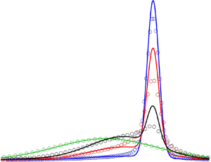
 $c_p=\sqrt {2}c_1$ in the free stream flow (region 1 in figure 1). Figures 7 and 8 present the results of comparison for local molecular velocity distribution functions for two values of normal Mach number. The M-S solution for the
 $\varphi$-attributes (
 $v_y^2$,
 $v_x^3$) is chosen for comparison because it is the most accurate variant of the solution in terms of predicting the DSMC macroparameters’ profiles. The comparison was carried out at points on the symmetry plane with the same density values in the DSMC and the M-S solutions (two values close to those in regions 1 and 3 and two intermediate values). The presented results of the comparison demonstrate qualitatively correct descriptions of the flow transition from state 1 to state 3 by the M-S approach for all considered normal Mach numbers.
Velocity distribution functions  $f(v_x)$ (a) and
 $f(v_y)$ (b) for
 $Ma_n=4.0$.

Velocity distribution functions  $f(v_x)$ (a) and
 $f(v_y)$ (b) for
 $Ma_n=10.0$.

For each case, dashed lines mark the values of the most probable velocity components  $U_i$ and
 $V_i$ for the modes of the corresponding solution (2.3). Let us consider the
 $x$-components of the velocities in more detail (see figures 7a and 8a). The value of
 $U_1$ for all the cases considered remains unchanged due to the constant value of the free stream Mach number. Changing of
 $Ma_{n}$ results in varying the values of
 $U_2=U_4$ and
 $U_3$. For the Mach number
 $Ma_n=4.0$, the relative differences of
 $U_2$ and
 $U_3$ from
 $U_1$ are 2.8 % and 4.4 %, respectively. The basis modes of the solution in this case are very close to each other. At the same time, as
 $Ma_n$ grows, these differences grow, which leads to an increase in the modality of the local solution. So, for
 $Ma_n=10.0$ the same differences reach 18.6 % and 31.1 %, respectively. This explains the decrease in quantitative differences between the DSMC and the M-S solutions. On the other hand, the modes in the DSMC distribution function turn out to be less pronounced for the intermediate values of density due to the presence of a large number of scattered molecules with velocities not representative of any Maxwellian mode. This strongly non-equilibrium effect is similarly observed in distribution functions inside normal shock waves (Pham-Van-Diep et al. Reference Pham-Van-Diep, Erwin and Muntz1989).
Strengthening of the modality of the velocity  $y$-component distributions can also be observed (see figures 7b and 8b): the increase in the normal Mach number leads to increasing the difference of
 $V_2$ and
 $V_4$ from the zero values of
 $V_1$ and
 $V_3$. However, this effect is less pronounced. Some quantitative differences for the intermediate density values are also clearly observed for this velocity component.
4. Conclusion
As stated above, the classical M-S analytical solution provides a qualitative approximate kinetic description of the internal structure of a 1-D normal shock wave. The results obtained in the present study demonstrate the possibility of applying a similar approach to the 2-D problem of the regular reflection of shock waves. The analytical M-S approximation provides a clear qualitative description of the evolution of macroparameters and molecular distribution functions along the plane of symmetry in this 2-D strongly non-equilibrium flow. The accuracy of the solution becomes better with increasing intensity of the incident shock wave.
Funding
The work on development of the Mott-Smith solution was supported by the Russian Science Foundation (grant no. 20-71-00114). The DSMC computations and the analysis of the accuracy of the Mott-Smith solution were carried out within the state assignment of Ministry of Science and Higher Education of the Russian Federation (project no. 121030500143-6). Computational resources of the Equipment Sharing Center ‘Mechanics’ of ITAM SB RAS were employed for the DSMC computations.
Declaration of interests
The authors report no conflict of interest.



