1. Introduction
Open cavity flows have been widely studied for their impinging shear layers, which represent the dominant phenomenon in the flow, see Rossiter (Reference Rossiter1964), Rockwell & Naudascher (Reference Rockwell and Naudascher1979), Rowley, Colonius & Basu (Reference Rowley, Colonius and Basu2002), Forestier, Jacquin & Geffroy (Reference Forestier, Jacquin and Geffroy2003), Larchevêque et al. (Reference Larchevêque, Sagaut, Mary and Labbé2003), Chang, Constantinescu & Park (Reference Chang, Constantinescu and Park2006), Basley et al. (Reference Basley, Pastur, Delprat and Lusseyran2013) among others. Such flows appear in many contexts, from mixing systems and coating techniques, to transport – think for instance of high-speed train top cavities, known to be the primary source of noise. Cavity flows belong to the family of impinging shear layers and meet the expectations of fundamental and applied research. However, it has been recently shown that the first instability does not occur in the shear layer but inside the cavity, as shown in Brès & Colonius (Reference Brès and Colonius2008), Meseguer-Garrido et al. (Reference Meseguer-Garrido, de Vicente, Valero and Theofilis2011), Alizard, Robinet & Gloerfelt (Reference Alizard, Robinet and Gloerfelt2012). As reported in these studies, frequencies associated with the inner-flow structures are approximately two orders of magnitude smaller than the dominant (shear-layer) frequencies (see also Basley et al. Reference Basley, Pastur, Delprat and Lusseyran2013, Reference Basley, Pastur, Lusseyran, Soria and Delprat2014). Indeed, fluid particle trajectories are bent when entering the recirculating flow inside the cavity, which may lead to the development of centrifugal instabilities. In such a case, the saturation of those instabilities actually gives rise to an alley of counter-rotating vortices, winding around the main recirculation flow, as was carefully described in Faure et al. (Reference Faure, Adrianos, Lusseyran and Pastur2007, Reference Faure, Pastur, Lusseyran, Fraigneau and Bisch2009). Basley et al. (Reference Basley, Pastur, Delprat and Lusseyran2013, Reference Basley, Pastur, Lusseyran, Soria and Delprat2014) addressed the coupling mechanisms between structures of the inner flow, characterised by a broad band of very low frequencies, and the shear-layer oscillations, characterised by well-defined frequencies two orders of magnitudes larger.
Centrifugal instabilities occur in a wide variety of flow configurations. Koseff & Street (Reference Koseff and Street1984a ,Reference Koseff and Street b ,Reference Koseff and Street c ) did a thorough study of the three-dimensional vortical structures observed in lid-driven cavities. In particular, visualisations of the flow highlighted the spatial periodic organisation of the vortices. Migeon (Reference Migeon2002) experimentally studied the mechanisms underlying the formation of the vortical structures. An analysis based on the Rayleigh criterion showed that lid-driven cavities actually develop Görtler instabilities, typical of open systems. However, the wavelength of the structure is twice the size of the unstable area, a feature typical of Taylor vortices, as observed in Taylor–Couette flow.
Lid-driven cavity flows present many similarities to open cavity flows. In open cavity flows, however, the inside flow recirculation is driven by the shear layer instead of the lid. It makes the dynamics more complex because couplings between the (fast) shear-layer oscillations and the (slow) space–time dynamics inside the cavity can occur, as has been shown in particular in the recent work by Basley et al. (Reference Basley, Pastur, Lusseyran, Soria and Delprat2014). Contrary to lid-driven cavities, few experimental studies exist exploring the dynamics developed inside open cavity flows. Maull & East (Reference Maull and East1963) was among the first to describe, in an experimental investigation, the three-dimensional organisation of the flow inside a rectangular open cavity, at small velocities. Faure et al. (Reference Faure, Adrianos, Lusseyran and Pastur2007) showed that the Görtler number associated with the inner counter-rotating vortices was in agreement with a Görtler-type instability. Here, again, the periodic organisation of these structures is typical of the Taylor instability. Like in lid-driven cavity flows, the inner patterns are therefore Taylor–Görtler-like structures. Faure et al. (Reference Faure, Pastur, Lusseyran, Fraigneau and Bisch2009) determined domains of existence of the inner-flow structures, as functions of the Reynolds number, streamwise and spanwise aspect ratios of the cavity. They reported an increase in the size of the structures with the streamwise aspect ratio and a slightly increase with the Reynolds number. Faure et al. (Reference Faure, Pastur, Lusseyran, Fraigneau and Bisch2009) also highlighted a slow drift of the structures towards the sidewalls. They showed, from direct numerical simulations of the three-dimensional flow, with and without rigid spanwise boundary conditions, that the drift was associated with secondary flows generated by rigid spanwise walls. A very similar drift was also observed in lid-driven cavities as a consequence of a secondary flow resulting from Bödewadt layers, as shown in Albensoeder, Kuhlmann & Rath (Reference Albensoeder, Kuhlmann and Rath2001), Albensoeder & Kuhlmann (Reference Albensoeder and Kuhlmann2006).
Although linear stability analysis cannot pretend to describe the full nonlinear dynamics of the flow, it can shed light on the constitutive elements of the dynamics at threshold. Several linear stability analyses were addressed for lid-driven cavities, among them Ding & Kawahara (Reference Ding and Kawahara1999), Albensoeder et al. (Reference Albensoeder, Kuhlmann and Rath2001), Theofilis, Duck & Owen (Reference Theofilis, Duck and Owen2004), Chicheportiche et al. (Reference Chicheportiche, Merle, Gloerfelt and Robinet2008), Boppana & Gajjar (Reference Boppana and Gajjar2010). Recent linear stability analyses of open cavity flows, in the incompressible regime, not only predict two-dimensional shear-layer modes to grow with positive growth rates, at reasonably high Reynolds numbers, but also predict the emergence of continuous families of three-dimensional modes inside the cavity, as shown in Brès & Colonius (Reference Brès and Colonius2008), Meseguer-Garrido et al. (Reference Meseguer-Garrido, de Vicente, Valero and Theofilis2011), Alizard et al. (Reference Alizard, Robinet and Gloerfelt2012), Meseguer-Garrido et al. (Reference Meseguer-Garrido, de Vicente, Valero and Theofilis2014). Dynamics inside the cavity develops over slow time scales, typically two orders of magnitude smaller than the time scales of shear-layer modes. Brès & Colonius (Reference Brès and Colonius2008), Meseguer-Garrido et al. (Reference Meseguer-Garrido, de Vicente, Valero and Theofilis2011, Reference Meseguer-Garrido, de Vicente, Valero and Theofilis2014) showed that the critical mode selected at threshold in fact depends critically on the cavity streamwise aspect ratio. In square cavities, Brès & Colonius (Reference Brès and Colonius2008), Meseguer-Garrido et al. (Reference Meseguer-Garrido, de Vicente, Valero and Theofilis2011, Reference Meseguer-Garrido, de Vicente, Valero and Theofilis2014), predict that the critical mode must belong to the family of steady growing modes. In the compressible regime, Brès & Colonius (Reference Brès and Colonius2008) showed that, for streamwise aspect ratios of 2 and 4, the critical mode is oscillatory. In the incompressible regime, Meseguer-Garrido et al. (Reference Meseguer-Garrido, de Vicente, Valero and Theofilis2011, Reference Meseguer-Garrido, de Vicente, Valero and Theofilis2014) showed that the critical mode is steady for aspect ratios up to approximately 1.2, whereas for aspect ratios larger than 1.2 the critical mode belongs to a family of oscillatory modes. Albensoeder et al. (Reference Albensoeder, Kuhlmann and Rath2001) found similar results for lid-driven cavity flows. Those linear stability analyses constitute a frame of reference for the present experimental study.
Up to now, no experimental study or direct numerical simulations has yet fully addressed the question of pattern selection in the centrifugal instabilities of open cavity flows in the incompressible regime, though linear stability analyses now predict families of modes towards which the base flow can destabilise. In this article, this question is addressed by reporting on the systematic experimental parametric study of the three-dimensional patterns selected at the threshold of the primary bifurcation. We show that different modes, either steady or unsteady, are actually selected at threshold depending on the streamwise aspect ratio of the cavity. We push the study even further and go beyond the primary threshold to see the emergence of new modes as the Reynolds number is increased, until a spatio-temporally chaotic dynamics eventually develops at large Reynolds numbers. The question of spanwise confinement, shown to have critical effects in many situations, and in particular in lid-driven cavity flow, is also addressed in this paper. In particular, the impact of the spanwise aspect ratio on pattern selection is studied experimentally and analysed in light of the secondary flows evidenced from direct numerical simulations conducted using the same conditions as the experiment.
The paper is organised as follows. In § 2, the experimental set-up is described. The generic space–time characteristics of the first bifurcated state are given in § 3. The parametric study of the bifurcation threshold evolution as a function of the aspect ratio, together with the analysis of the criticality of the bifurcation, are given in § 3.3. We identified families of modes, the selection of which at threshold critically depends on the cavity aspect ratio, as shown in §§ 3.2 and 3.4. We discuss these results with respect to expectations from linear stability analyses of the flow in § 4.3. It is shown that secondary flows can give rise to additional dynamical features of the patterns. Section 4.1 is dedicated to the analysis of such secondary flows, and their impact on the selected patterns, in a cavity of small aspect ratio, by means of direct numerical simulations. It is also shown in lid-driven cavities that the spanwise confinement can have a strong impact on pattern selection at threshold. Section 4.2 is devoted to the study of spanwise confinement on pattern selection, by doubling the cavity depth, in order to reduce the cavity spanwise aspect ratio by a factor two. In addition, as the Reynolds number is increased, it is expected that the dynamics becomes much more complex and may exhibit features of space–time chaos. Section 5 is dedicated to the complex space–time dynamics of the inner flow at larger Reynolds numbers. Finally, we give an overall summary of this study in the concluding section.
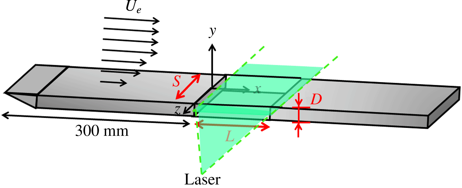
Scheme of the experimental set-up.

2. Experimental set-up
The experimental facility is a wind tunnel composed of a centrifugal fan, located upstream of a calming section, and the test section. The calming section includes a settling chamber followed by a convergent and two honey-comb panels at the inlet of the contraction in order to laminarise the flow. Vein noise has been estimated on the basis of laser Doppler velocimetry (LDV) measurements. Background turbulence is less than 1 %. The wind tunnel forces frequencies mainly distributed from 0 to 10 Hz, with a maximal power, at around 1 Hz, three orders of magnitude smaller than the cavity flow spectrum for the same frequency range. A sketch of the test section configuration is shown in figure 1. The span of the wind tunnel is
 $S=300~\text{mm}$
, while the top to bottom distance is
 $75~\text{mm}$
, the top and bottom boundary layers therefore never meet. This study focuses on two cavity depths, namely
 $D=25~\text{mm}$
and
 $D=50~\text{mm}$
, reciprocally corresponding to span aspect ratios
 $S/D=12$
and
 $S/D=6$
. The cavity length
 $L$
will be varied from
 $L/D=1$
to 2. Aspect ratios
 $L/D=1$
and 1.1 are missing for the case
 $S/D=12$
, as summarised in table 1, because the very small streamwise size of the cavity allows neither visualisations by smoke nor LDV access to the inner flow. The origin of the coordinate system is chosen midspan of the upstream edge. The
 $x$
-axis is in the direction of the external flow, the
 $y$
-axis is normal to the floor of the cavity and the
 $z$
-axis is in the spanwise direction (see figure 1).
The origin of the boundary layer is fixed by an elliptical leading edge,
 $300~\text{mm}$
upstream of the cavity entrance edge, where a quasi-Blasius velocity profile develops (form factor
 $h\approx 2.3$
). The laminar momentum thickness
 ${\it\theta}_{0}$
depends on the incoming velocity
 $U_{e}$
and never exceeds a few millimetres.
Centrifugal instabilities develop at very low incoming velocities, typically less than
 $1~\text{m}~\text{s}^{-1}$
. In wind tunnels, such low velocities are challenging with respect to flow rate regulation. The incoming velocity stability is approximately
 $0.025~\text{m}~\text{s}^{-1}$
, a value which therefore constitutes the lower limit of the velocity step used for the determination of the instability thresholds.
Aspect ratios
 $L/D$
investigated in the cavity of spanwise aspect ratio
 $S/D=12$
.

Complete optical access is made available using reflection-treated glass walls for the test section and the cavity, in order to allow particle image velocimetry (PIV) and LDV. The cavity itself consists of three distinct rectangular elements in coated glass. The first element is a forward-facing step at the inlet of the test section, much deeper than the cavity depth. The second element is the base floor used to impose the cavity depth
 $D$
. The third element is a
 $D$
-deep backward-facing step which can slide above the flat floor of the second element, so as to adjust the cavity length
 $L$
.
Note that the flow appears to be quite sensitive to inaccuracies in the cavity assembly. Therefore, we had to pay particular attention to suppress any leaks that could be present at the edges and corners of the cavity.
Velocity fields are obtained by PIV mainly in a (
 $x,z$
)-plane located at
 $y/D=-0.30$
. The laser sheet is produced by
 $200~\text{mJ}$
Quantel twin-pulsed YAG lasers. A standard, single-frame video camera (AVT Cameras – Marlin,
 $1024\times 768$
pixel of size
 $4.65~{\rm\mu}\text{m}\times 4.65~{\rm\mu}\text{m}$
with a resolution depth of
 $8$
bit) acquires images of particles at a frame rate of
 $20$
Hz. An electronic delay-generator (R&D Vision) is used to synchronise the flash lamps and Q-switches of both laser cavities together with the camera chronogram and, when required, LDV recordings, with a precision of
 $0.5~{\rm\mu}\text{s}$
.
Velocity fields,
 $\boldsymbol{v}(\boldsymbol{r},t)$
, are computed from a pair of images by using an orthogonal dynamical-programming optical flow algorithm, following Quénot, Pakleza & Kowalewski (Reference Quénot, Pakleza and Kowalewski1998). The velocity field repetition rate is
 $f_{e}=10$
Hz. Consequently, the Shannon–Nyquist frequency is 5 Hz, greater than the highest characteristic frequency of the inner-flow dynamics (order of 1 Hz). Airflow is seeded with micrometric droplets of DEHS (Di-Ethyl-Hexyl-Sebacat). Smoke visualisations are also carried out in the PIV plane.
LDV measurements are carried out with a DANTEC BSA system using a
 $35~\text{mW}$
continuous laser at
 $660~\text{nm}$
with a front lens of focal length
 $300~\text{mm}$
. A Bragg cell, modulated at
 $80$
MHz, allows the detection of any changes in the velocity sign, up to
 $267~\text{m}~\text{s}^{-1}$
. The interferometric fringe interval is
 $3.335~{\rm\mu}$
m and the measurement volume (
 ${\it\delta}x\times {\it\delta}y\times {\it\delta}z\simeq 0.1\times 0.1\times 1.0~\text{mm}^{3}$
) contains approximately thirty fringes. The cross-flow velocity component
 $u_{y}$
is measured at
 $x/L=0.18$
,
 $y/D=-0.24$
and
 $z/S=-0.15$
for
 $S/D=12$
, and
 $x/L=0.38$
,
 $y/D=-0.102$
and
 $z/S=0.087$
for
 $S/D=6$
.
Strouhal numbers are defined as
 $St=fD/U_{e}$
, where
 $f$
is the frequency, and Reynolds numbers as
 $Re=D\,U_{e}/{\it\nu}$
, where
 ${\it\nu}=15\times 10^{-6}~\text{m}^{2}~\text{s}^{-1}$
is the kinematic viscosity of air.
Frequencies in this paper concern only the dynamics of the three-dimensional structures present inside the cavity, Reynolds numbers being smaller than the critical value of the shear-layer self-sustained oscillations, if not quoted otherwise.
In order to extract the spatial field associated with a given spectral frequency, dynamic mode decomposition (DMD) is performed on the fluctuating velocity field following Schmid (Reference Schmid2010). In the frame of this study, dynamic modes are closely similar to global Fourier modes, as shown in Chen, Tu & Rowley (Reference Chen, Tu and Rowley2012), Basley et al. (Reference Basley, Pastur, Delprat and Lusseyran2013).
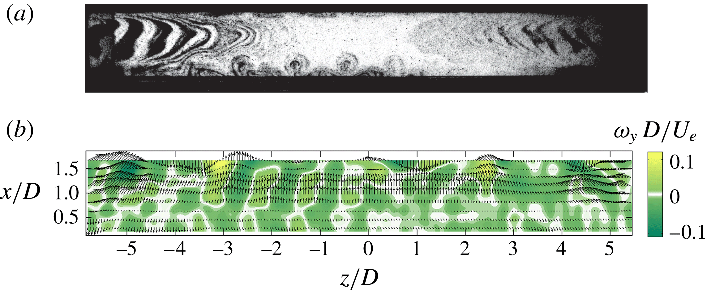
Dynamics observed in an horizontal plane: (a) smoke visualisation (
 $y/D=-0.3$
) for
 $S/D=12$
,
 $L/D=1.75$
and
 $Re_{D}=2000$
, (b) instantaneous vorticity field in an horizontal plane (
 $y/D=-0.3$
) for
 $S/D=12$
,
 $L/D=1.75$
and
 $Re_{D}=1863$
.

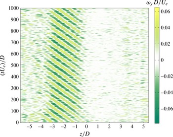
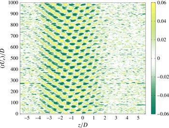
Space–time diagram built from a vorticity line in
 $x/D=1$
for
 $S/D=12$
,
 $L/D=1.75$
,
 $Re_{D}=1863$
.

3. Inner-flow structure beyond threshold
In this section, we consider the case
 $S/D=12$
. For such a configuration, the dynamics exhibits most of the generic features that will be discussed in reference to the literature. Smaller spans will introduce confinement effects that will be discussed in § 4.2.
3.1. Flow phenomenology
The first bifurcated state takes the form of an alley of pairs of counter-rotating vortical structures, each pair forming a ring around the main recirculation flow. Smoke visualisation of figure 2(a), in an horizontal plane below the cavity top plane, exhibits mushroom-like structures (at the bottom of the figure), which are typical of the bifurcated state (Faure et al. Reference Faure, Pastur, Lusseyran, Fraigneau and Bisch2009). The arrowhead-like striped pattern, from the edges of the picture to the centre of the cavity, is the trace of a cyclic injection of smoke by the mixing-layer oscillations. Note that this process can often occur below the onset of self-sustained oscillations, with the power spectra exhibiting an energy distribution typical of the Kelvin–Helmholtz instability triggered by white noise. The slow displacement of the streak lines towards the centre of the cavity reveals the large time scales of the inner flow. The frontier between the flows inside (striped patterns) and outside (mushroom-like patterns) of the main recirculation core is clearly delineated, which means that mixing between these two areas is weak.
In figure 2(b) are shown both the planar velocity field (arrows) and the cross-wise vorticity field (colour). The wavelength of the vortical pattern scales as the cavity depth. A space–time diagram of the dynamics, based on the vorticity field at
 $x/D=1$
, is shown in figure 3, for aspect ratio
 $L/D=1.75$
. In this case, it clearly exhibits a left-travelling wave, with a spatially bounded envelope, between approximately
 $z/D=-4$
and
 $z=0$
. Well-defined stationary left and right fronts mark out the wavepacket. However, it can also occur that the waves spread over the entire span, as shown in Faure et al. (Reference Faure, Pastur, Lusseyran, Fraigneau and Bisch2009). Most often, left-travelling waves to the left and right-travelling waves to the right coexist in space, separated by a source-like singularity, Faure et al. (Reference Faure, Pastur, Lusseyran, Fraigneau and Bisch2009). In the present study, however, the structures were always localised in space. In addition, travelling waves, when excited, were systematically either left- or right-travelling at threshold, depending on the aspect ratio. This feature, and others to be discussed later on, strongly suggests the existence of an experimental bias. We suspect the bias to be due mainly to a non-symmetrically uniform incoming flow, upstream of the cavity. However, as we will see, the bias does not fundamentally change the phenomenology of the flow, but as its main consequence unfolds the bifurcation by breaking the symmetry of the base flow.
3.2. Families of modes
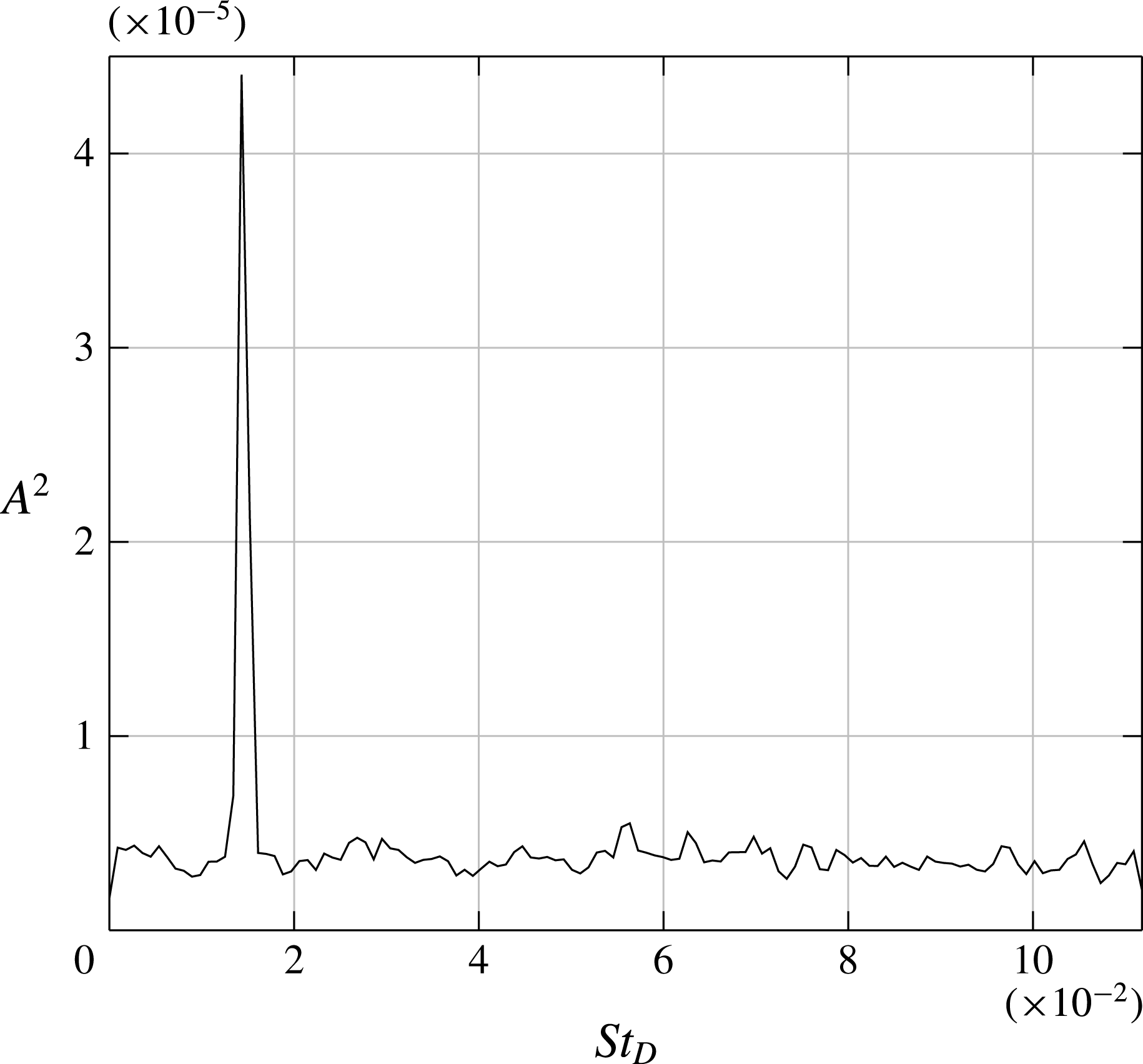
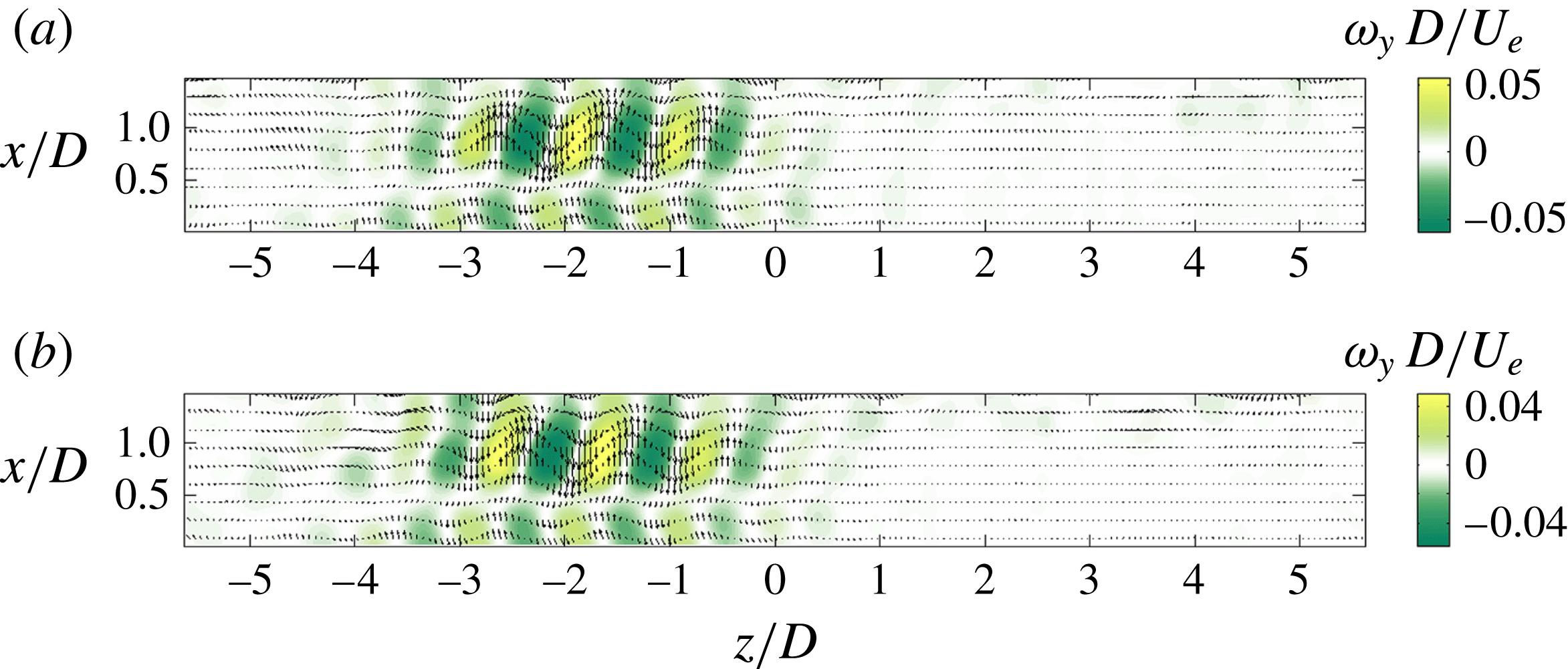
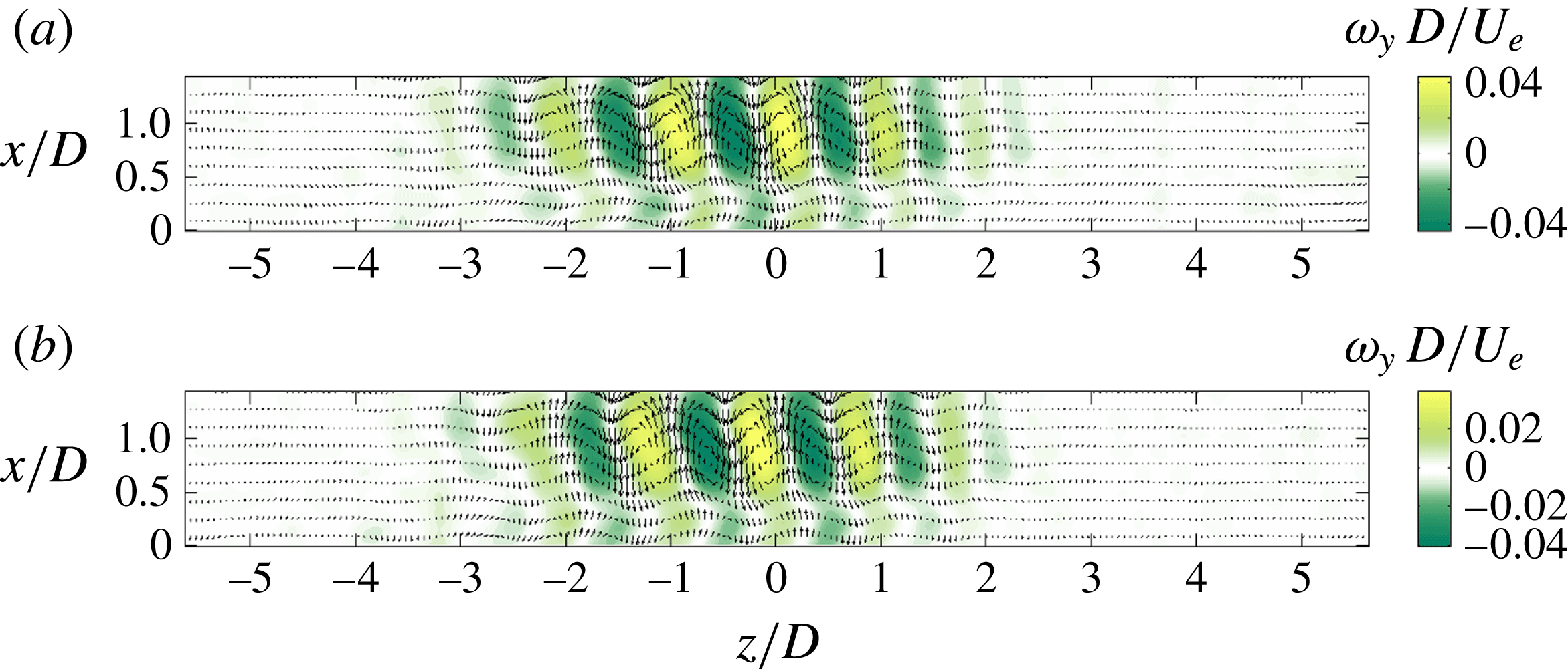
The primary bifurcation is characterised by the appearance of drifting structures. Consequently, we can take advantage of the associated peak (see figure 4) in the power spectral density of a local LDV measurement to study the onset of the bifurcation. For the sake of illustration, the dynamic mode associated with the dominant peak in the power spectrum of figure 4 is shown in figure 5. Both the real and imaginary parts of the mode look very similar, though slightly shifted in space, as expected for a left-travelling wave. The dynamics of this mode can be observed in movie 1 available online at http://dx.doi.org/10.1017/jfm.2015.726.
Power spectral density for
 $S/D=12$
,
 $L/D=1.75$
,
 $Re_{D}=1863$
, from the streamwise component of the velocity field, averaged over the spatial PIV domain.

Real part (a) and imaginary part (b) of the dynamic mode associated with
 $St_{D}=0.015$
(
 $f=0.66~\text{Hz}$
) for
 $S/D=12$
,
 $L/D=1.75$
,
 $Re_{D}=1863$
. Planar velocity (
 $u_{z},u_{x}$
) field (arrows) on the top of the cross-wise vorticity field
 ${\it\omega}_{y}$
(colour).

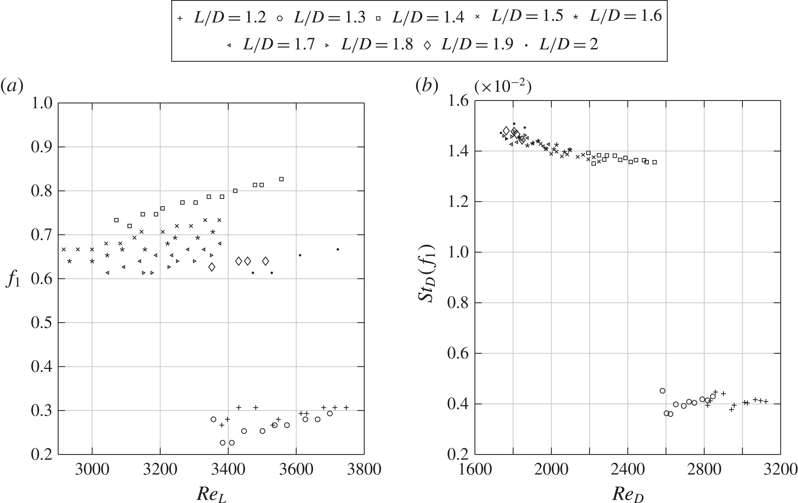
Evolution of (a) frequency and (b) Strouhal number of the propagating wave, as a function of the Reynolds number (where
 $Re_{L}=U_{e}L/{\it\nu}$
) for the different
 $L/D$
.

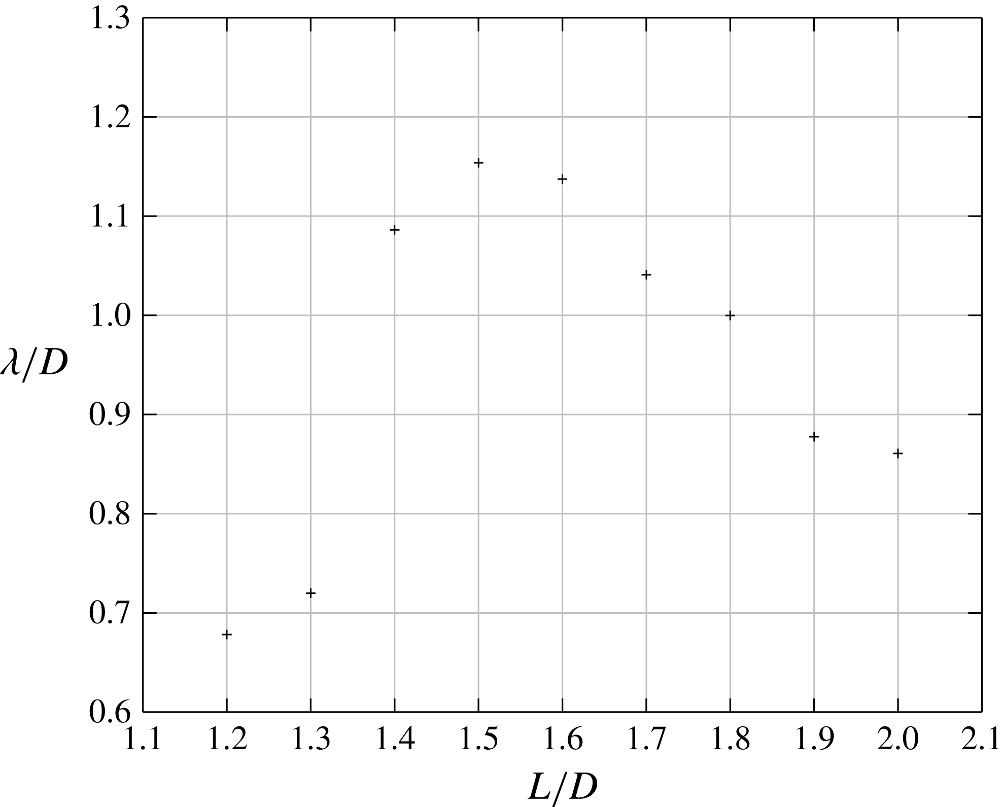
Wavelength evolution with aspect ratio
 $L/D$
for
 $S/D=12$
. Threshold gap
 ${\it\epsilon}=\sqrt{Re-Re_{c}}=0.042$
for
 $L/D=1.2$
and 1.5,
 ${\it\epsilon}=0.037$
for
 $L/D=1.3$
and
 $1.4$
,
 ${\it\epsilon}=0.030$
for
 $L/D=1.6$
and
 $1.7$
,
 ${\it\epsilon}=0$
for
 $L/D=1.8$
,
 $1.9$
and
 $2$
.

The evolution of the Strouhal number with
 $L/D$
is presented in figure 6. The Strouhal number is of the order of
 $0.014$
for aspect ratios
 $L/D$
larger than 1.3. This order of magnitude is in good agreement with frequencies of the propagating modes identified in Brès & Colonius (Reference Brès and Colonius2008), Faure et al. (Reference Faure, Pastur, Lusseyran, Fraigneau and Bisch2009), Meseguer-Garrido et al. (Reference Meseguer-Garrido, de Vicente, Valero and Theofilis2011, Reference Meseguer-Garrido, de Vicente, Valero and Theofilis2014), Basley et al. (Reference Basley, Pastur, Lusseyran, Soria and Delprat2014). More noticeable is the break in Strouhal number around
 $L/D\simeq 1.3$
. In cavities of small aspect ratios (
 $L/D\leqslant 1.3$
), Strouhal numbers are of the order of
 $St_{D}\approx 4\times 10^{-3}$
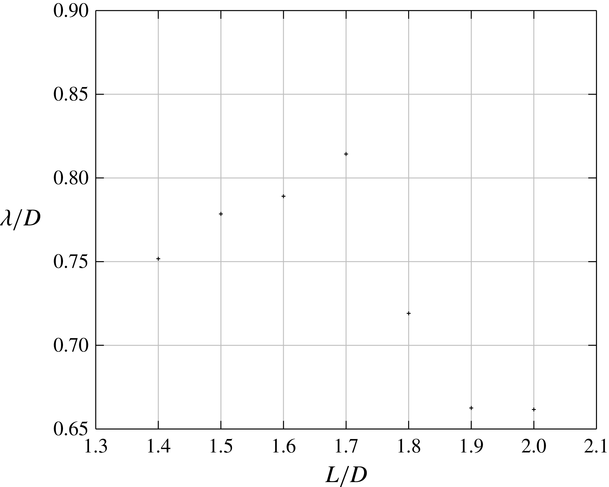
, that is, one order of magnitude smaller than the Strouhal numbers found for longer cavities. A sudden jump in the wavelength evolution is also observed around
 $L/D\simeq 1.3$
, as shown in figure 7. Wavelengths are determined by dividing the drift velocity, measured in space–time diagrams, by the drift frequency, measured by LDV. In agreement with Faure et al. (Reference Faure, Pastur, Lusseyran, Fraigneau and Bisch2009), we checked that the wavelengths, though not strictly determined at the same distance to threshold in the different configurations, do not significantly vary over the range of values considered. For
 $L/D\leqslant 1.3$
it is found that
 ${\it\lambda}/D\simeq 0.7$
, while for
 $L/D\geqslant 1.4$
wavelengths are larger,
 ${\it\lambda}/D>0.85$
, with a maximum value
 ${\it\lambda}/D=1.15$
for
 $L/D=1.5$
. Note, in figure 6(a), that, for a fixed value of the Reynolds number, the (dimensioned) frequency first decreases when the aspect ratio increases, before it eventually reaches an asymptotic value for
 $L/D>1.5$
.
The discontinuity in the evolution of the Strouhal number and wavelength suggests that the family of modes selected at threshold is not the same owing to the aspect ratio
 $L/D$
. For aspect ratios
 $L/D\leqslant 1.3$
, a family of quasisteady modes is selected with a wavelength approximately half the cavity depth, while for
 $L/D\geqslant 1.4$
the mode is oscillatory, with a wavelength of the order of the cavity depth.
3.3. Threshold of centrifugal instability
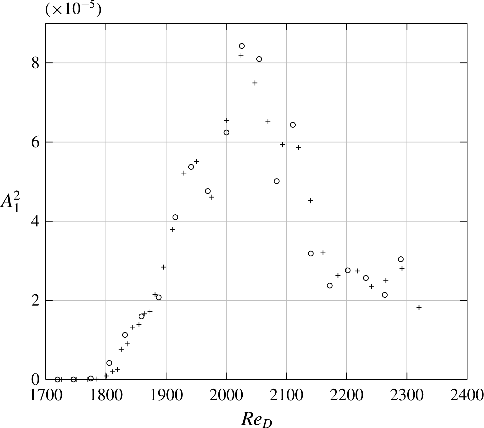
Power spectral density evolution of the primary mode with the Reynolds number for
 $S/D=12$
and
 $L/D=1.75$
, under increasing (
 $+$
) and decreasing (○) ramps of the external velocity. The probe is located at
 $x/L=0.38$
,
 $y/D=-0.88$
and
 $z/S=0.007$
. Power spectral densities are estimated using a Welch method, with time windows
 $50~\text{s}$
large and
 $99\,\%$
overlapping (Welch Reference Welch1967).

Evolution of the power density with the Reynolds number for several aspect ratios
 $L/D$
. The LDV probe is located at
 $x/L=0.178$
,
 $y/D=-0.24$
,
 $z/S=-0.15$
. Power spectral density is calculated with a time window
 $75~\text{s}$
wide, for a total observation time of
 $120~\text{s}$
, and a window overlapping of
 $99\,\%$
.

Bifurcation thresholds for
 $S/D=12$
: (a) bifurcation threshold of the first travelling wave depends on
 $L/D$
: spectral criterion (
 $+$
) and criterion based on smoke visualisation (▫); (b) bifurcation thresholds of the right-travelling (
 $+$
for
 $L/D<1.4$
and ○ for
 $L/D\geqslant 1.4$
) and left-travelling (▫) waves.

The critical Reynolds number
 $Re_{c}$
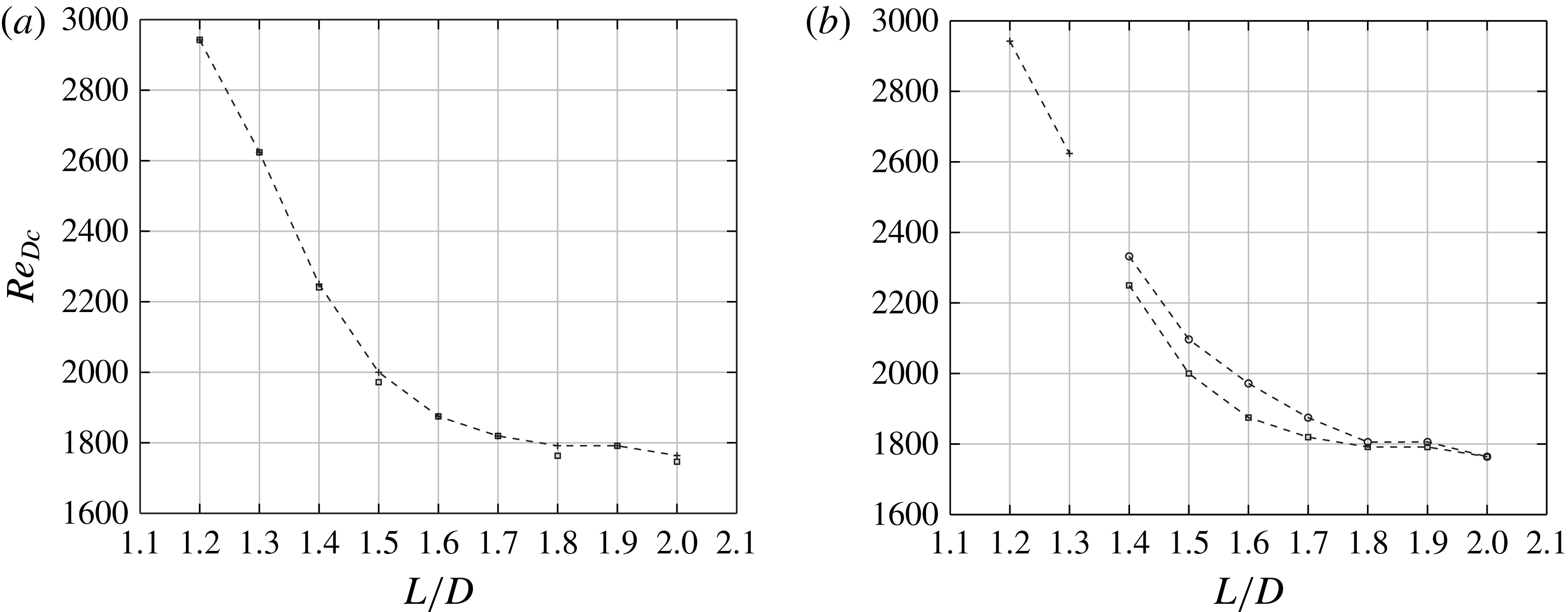
is determined by extrapolating to zero the power density as the Reynolds number is varied, while the criticality of the bifurcation is determined by comparing the critical Reynolds numbers of decreasing, followed by increasing, ramps of the velocity. With a fairly good reproducibility, the onset values determined by visual inspection of the smoke field are almost undistinguishable from those determined with the more precise methodology based on spectral power. Therefore, we sometimes preferred to determine onsets from smoke visualisations, which are faster to conduct, in order to increase the number of individual experiments. Figure 8 shows the evolution of the power spectral density during both increasing and decreasing ramps of the Reynolds number, for
 $L/D=1.75$
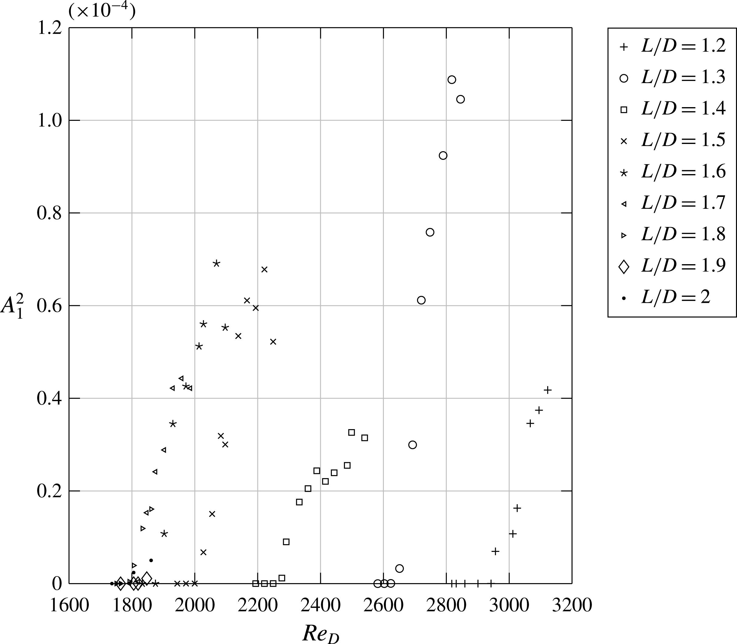
. In both cases, the thresholds are found to be the same, at the precision of the experiment. This lack of hysteresis is also found for all
 $L/D$
ratios studied, as shown in figure 9, suggesting supercritical bifurcations.
As shown in figure 10, the threshold value decreases when the cavity length increases. It means that the inner flow, in square cavities, is more robust against centrifugal instabilities than in rectangular cavities. In particular, the critical Reynolds number decreases towards some asymptotic value
 $Re_{c}=Re_{\infty }$
, where
 $Re_{\infty }\simeq 1750$
, for
 $L/D>1.6$
. The trend in figure 10 is in close agreement with the monotonic decrease of the threshold predicted from the linear stability analyses of open cavity flows conducted in Meseguer-Garrido et al. (Reference Meseguer-Garrido, de Vicente, Valero and Theofilis2011, Reference Meseguer-Garrido, de Vicente, Valero and Theofilis2014). Note that the same behaviour was found for lid-driven cavities, see e.g. Theofilis et al. (Reference Theofilis, Duck and Owen2004).
Spanwise vorticity field
 $\overline{{\it\omega}}_{z}(x,y)$
, in the vertical plane
 $z/D=0.01$
, averaged over 980 PIV fields, for
 $S/D=12$
,
 $L/D=1.75$
,
 $Re_{D}=2700$
. The circle approximately indicates the solid rotating core.

Brès & Colonius (Reference Brès and Colonius2008) claimed that the reversal time of the main recirculation provides the time scale for the dynamics of the spanwise mode. We compared both time scales from synchronised PIV measurements in two planes, vertical and horizontal, for the configuration
 $L/D=1.75$
. The reversal time frequency
 $f_{rev}={\it\Omega}/2{\rm\pi}\simeq \overline{{\it\omega}}_{z}/4{\rm\pi}$
can be extracted from the value of the spanwise component
 $\overline{{\it\omega}}_{z}$
of the mean vorticity field, in the core of the mean recirculation flow, which is assumed to be in solid rotation with angular velocity
 ${\it\Omega}$
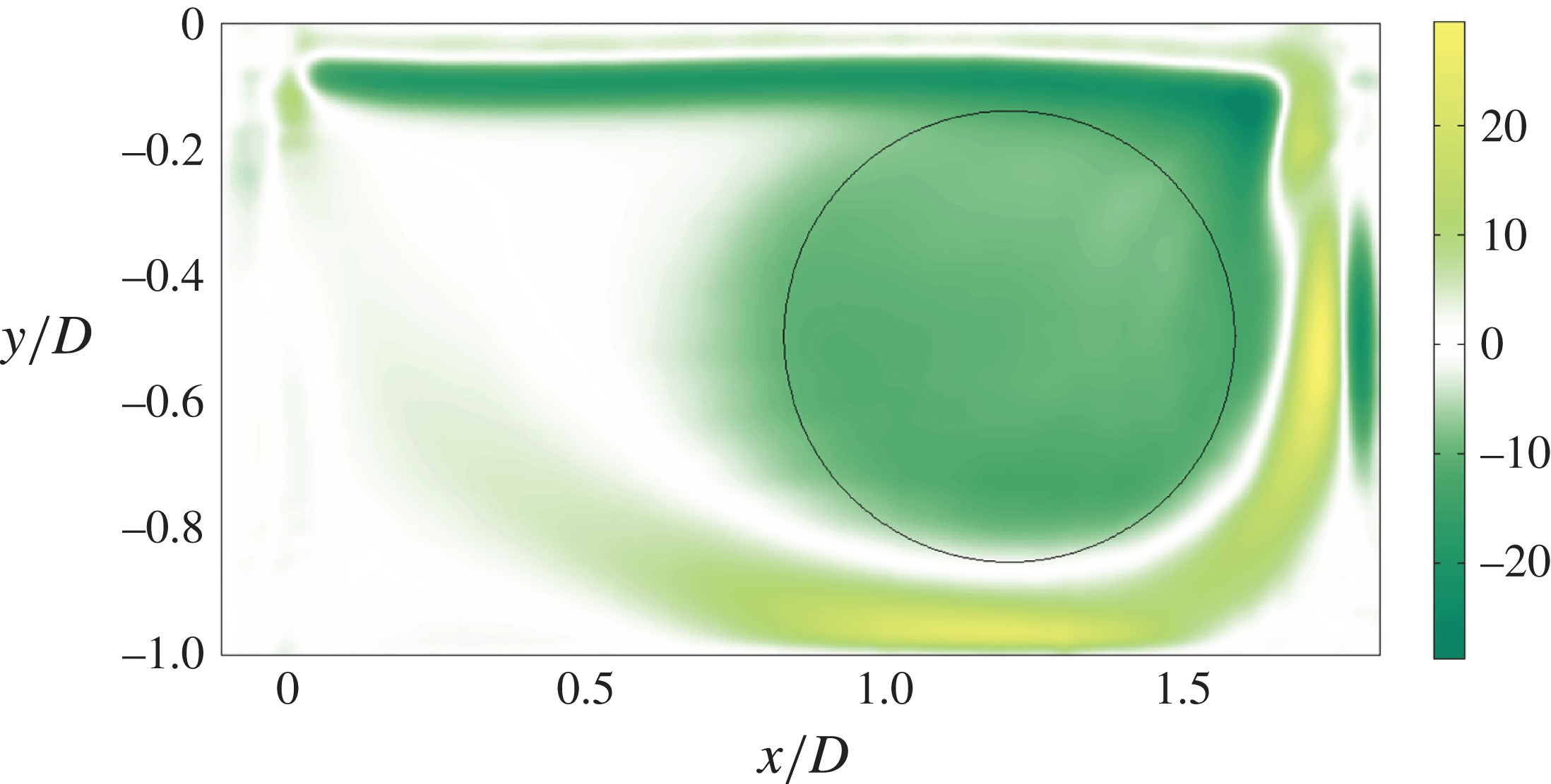
, as shown in Chattelier, Laumonier & Gervais (Reference Chattelier, Laumonier and Gervais2004). The reversal time frequency is estimated by averaging the vorticity field over the solid rotation core, indicated by the surface of the circle drawn in figure 11. It is estimated to approximately
 $0.77~\text{Hz}$
(
 $St_{D}=0.011$
), comparable to the dominant frequency associated with the left-travelling mode at
 $St_{D}=0.012$
. Both are in fair agreement. When the cavity length is increased, the reversal time of the main recirculation increases too, and the mode frequency should therefore decrease, as observed in figure 6(a).
In the range of Reynolds numbers where the power spectral density is linearly increasing, both supercritical fork (
 $L/D\leqslant 1.3$
) and Hopf (
 $L/D\geqslant 1.4$
) bifurcations may be described, at the lowest (non-trivial) order in the spectral amplitude
 $A$
, by a Stuart–Landau equation (Manneville Reference Manneville and Scott2005):
 $$\begin{eqnarray}\displaystyle {\it\tau}{\dot{A}}={\it\epsilon}A-{\it\beta}|A|^{2}A, & & \displaystyle\end{eqnarray}$$
where the growth rate
 ${\it\epsilon}=\sqrt{Re-Re_{c}}$
is the threshold gap and
 ${\it\beta}$
is the coefficient of nonlinear self-saturation. In case of a fork bifurcation,
 $A$
is a real-valued amplitude, while
 $A$
would be complex for a Hopf bifurcation. The power density at saturation follows as
 $|A_{s}|^{2}={\it\epsilon}/{\it\beta}$
. From figure 9, it can be seen that the slope of the curve
 $|A_{s}|^{2}$
, as a function of
 $Re-Re_{c}$
, is almost independent of
 $L/D$
, and
 $1/{\it\beta}\simeq 3\times 10^{-7}$
in units of the power spectral density. Note that the previous discussion does not directly apply to the cavity of aspect ratio
 $L/D=1.4$
, since, in that case, the power density does not evolve linearly with
 $Re-Re_{c}$
(see figure 9). This configuration is in fact close to a co-dimension two bifurcation point.
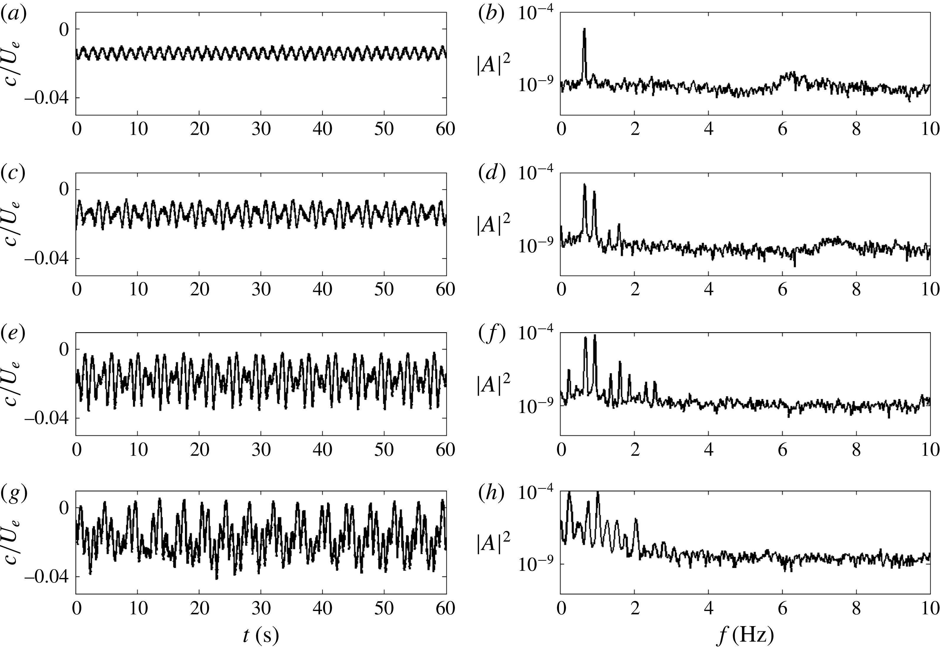
Finally, it is worthwhile noticing that the power spectral density, in figure 8, appears to evolve erratically as the Reynolds number is increased beyond the linear growth regime. However, the evolution of the power is fully deterministic, since the same behaviour is found in both increasing and decreasing ramps of the Reynolds number. We will come back to this point in § 5.
3.4. Imperfect Hopf bifurcation
When the Reynolds number is increased slightly beyond the onset of the primary bifurcation, for aspect ratio
 $L/D\geqslant 1.4$
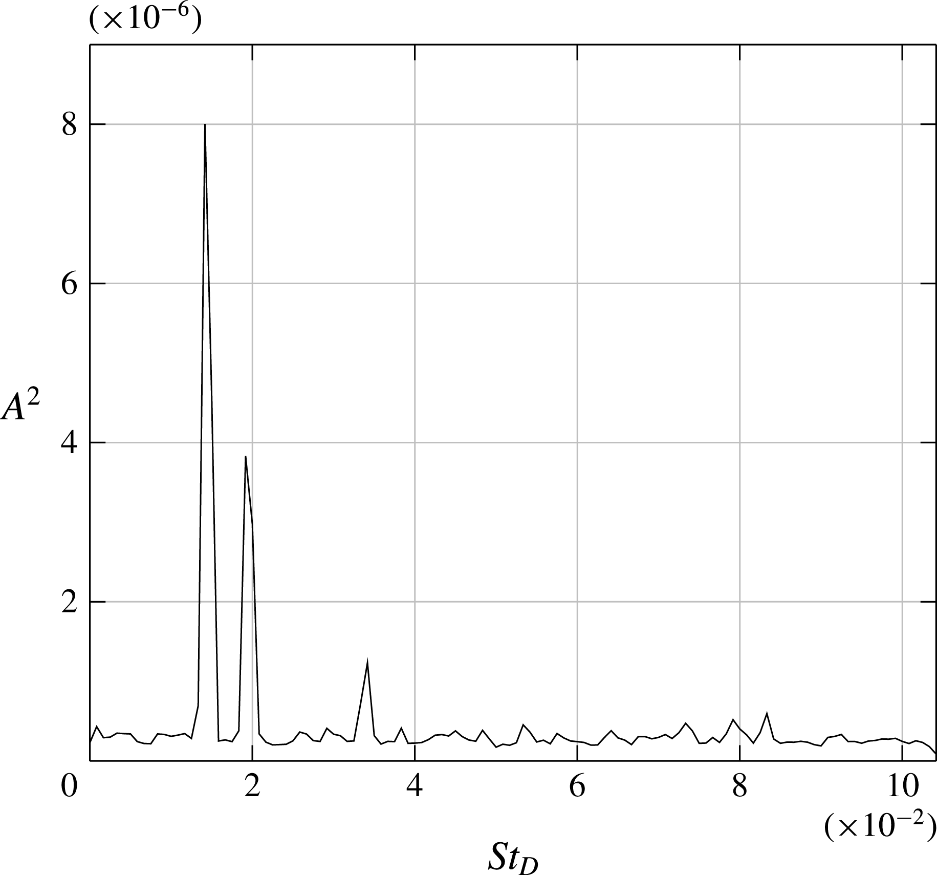
(family of propagating modes), a new peak emerges in the power spectral density, rising continuously from zero, as shown from the PIV measurement in figure 12 for the case
 $L/D=1.75$
. The new frequency is systematically found to be different from the frequency of the dominant mode, as exemplified in figure 12 for
 $L/D=1.75$
, where the dominant frequency is found at a Strouhal number of approximately
 $St_{D}=0.015$
(
 $f_{1}=0.70~\text{Hz}$
) while the emerging peak is found at
 $St_{D}=0.020$
(
 $f_{2}=0.94~\text{Hz}$
). A DMD analysis shows that the secondary peak is the signature of a right-travelling wave, with a finite spatial extension, as shown in figure 13. The dynamics of this mode can be observed in the supplementary movie 2. The wavelength of the new mode, at threshold, is shown in figure 14 as a function of the aspect ratio. The threshold of occurrence of the secondary peak, as a function of the aspect ratio, is found to be very close to the onset of the primary bifurcation, as shown in figure 10(b). The relative gap is less than
 $5\,\%$
. We argue that the experimental bias causes the slight gap between both thresholds, but also breaks the symmetry between the left- and right-travelling waves, which would otherwise be symmetrical waves.
The left- and right-travelling waves are superimposed in space, giving rise locally to a quasistationary wave in the space–time diagram of figure 15. The nodes of the stationary wave drift slowly to the right, mainly due to the small frequency shift
 ${\rm\Delta}f=f_{2}-f_{1}>0$
between the two travelling waves. Note that the left-travelling waves alone exist close to the left sidewalls, which is consistent with a finite-geometry effect as reported in Cross (Reference Cross1986). The dynamics of the left and right propagating waves superimposition can be observed in the supplementary movie 3.
Power spectral density for
 $Re_{D}=2000$
,
 $S/D=12$
and
 $L/D=1.75$
from the streamwise component of the velocity field, averaged over the spatial PIV domain.

Real and imaginary parts of the dynamic mode associated with
 $St_{D}(f_{2})=0.020$
(
 $f_{2}=0.94~\text{Hz}$
) for
 $S/D=12$
,
 $L/D=1.75$
and
 $Re_{D}=2000$
. Planar velocity (
 $u_{z},u_{x}$
) field (arrows) on the top of the cross-wise vorticity field
 ${\it\omega}_{y}$
(colour).

Wavelength evolution of the right-travelling wave with
 $L/D$
for
 $S/D=12$
.

Space–time diagram built from a vorticity line in
 $x/D=1$
for
 $Re_{D}=2000$
,
 $S/D=12$
and
 $L/D=1.75$
.

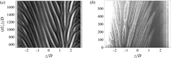
Space–time diagram build from the (a) streamwise velocity component at
 $x/D=0.25$
and
 $y/D=-0.6$
, from DNS, and (b) smoke visualisations along the line
 $x/D=0.7$
and
 $y/D=-0.16$
, from experiment.

4. Discussion
4.1. Steady mode drift at small aspect ratios
In our experiment, the structures observed for small aspect ratios, though slowly drifting, are not steady. Such a drift was reported in Faure et al. (Reference Faure, Pastur, Lusseyran, Fraigneau and Bisch2009) in the case of rigid boundary conditions, while the drift stops with periodic boundary conditions. The drift was interpreted as resulting from end-wall effects. In this section, we address the question of the end-wall effects and estimate the order of magnitude of the mean secondary flows near the end walls.
In order to remove any undesirable experimental bias from the analysis, we performed direct numerical simulations of an open square cavity flow, with
 $L/D=1$
and
 $S/D=6$
at
 $Re_{D}=4230$
. The incompressible isothermal Navier–Stokes equations are solved with the OLORIN code, see Podvin et al. (Reference Podvin, Fraigneau, Lusseyran and Gougat2006). The mesh is composed of
 $256\times 128\times 128$
Cartesian cells, refined close to the walls and in the shear layer. We impose no-slip boundary conditions in order to mimic the experimental configuration. More information about the numerical details can be found in Pastur et al. (Reference Pastur, Fraigneau, Lusseyran and Basley2013). The space–time diagram of figure 16(a) exhibits striking similarities to the experimental space–time diagram of figure 16(b). In particular, the source from which left- and right-travelling waves emanate is not located in the symmetry plane of the cavity. It is located at
 $z/D=1.5$
in figure 16(a), and at
 $z/D\simeq -1.5$
in the experimental run of figure 16(b). In the space–time plot of figure 16(a), the drift velocity to the left is approximately
 $c/U_{e}=1.1\times 10^{-3}$
(
 $c\simeq 1.5~\text{mm}~\text{s}^{-1}$
) for
 $-3<z/D<1,5$
, whereas the drift velocity to the right is approximately
 $c/U_{e}=1.3\times 10^{-3}$
for
 $1,5<z/D<3$
. Close to the spanwise walls, the drift accelerates to velocities of approximately
 $5~\text{mm}~\text{s}^{-1}$
, i.e
 $c/U_{e}=3.9\times 10^{-3}$
. In addition, the wavelength changes slowly with
 $z$
. It increases to
 $0.8\,D$
in the close vicinity of the source, and decreases to
 $0.6D$
away from the source. These values of the wavelength, together with the Strouhal number
 $St=cD/({\it\lambda}U_{e})\simeq 0.002$
, are those actually experimentally identified for the quasisteady modes (
 $L/D\leqslant 1.3$
).
Note that the space–time diagram of figure 16(b) looks very similar to those reported in Burguete, Mancini & Pérez-Garcia (Reference Burguete, Mancini and Pérez-Garcia1993) in the case of a Bénard–Marangoni convection with spatially inhomogeneous heating, where the bias there is deliberately imposed on the system.
Top view of the spanwise velocity component of the time-averaged velocity field in the (
 $x,z$
) plane at
 $y/D=-0.6$
for
 $L/D=1$
and
 $S/D=6$
, from DNS. Note that the mean field is not fully converged due to the very slow time scales of the dynamics.

Spanwise velocity profile in
 $y/D=-0.6$
averaged over
 $x/D$
from 0 to 0.25, for
 $L/D=1$
and
 $S/D=6$
, from DNS.

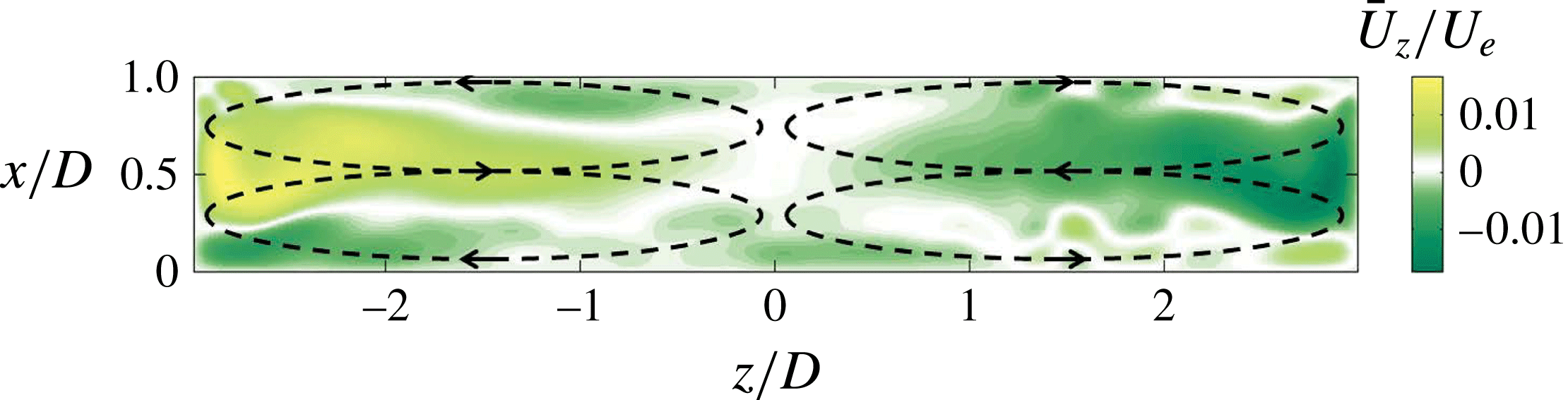
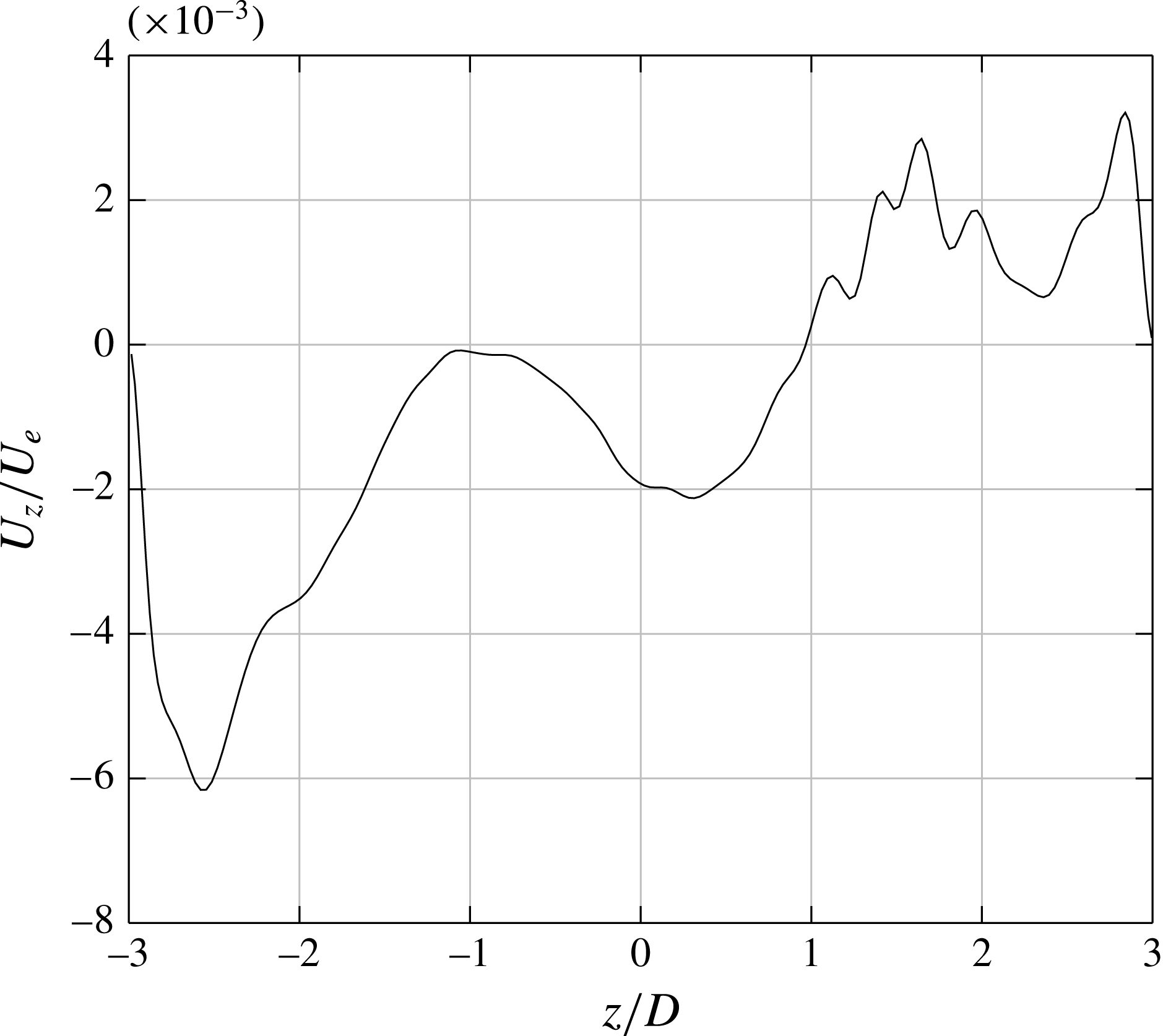
The question we would like to address now is whether the slow motion of the structures towards the spanwise boundaries, in small aspect ratio cavities, could be the trace of an underlying secondary flow oriented towards the end walls that would carry the steady mode. Consider the mean field of figure 17, obtained by time averaging the velocity fields. The secondary flows form four recirculation cells, symbolised by the dotted lines. Pumping by the end walls settles close to the upstream and downstream walls, while fluid reinjection settles at the centre of the cavity with much larger velocities. Consider the velocity spanwise component
 $w(z)$
, averaged over the pumping area,
 $x/D\in [0,0.25]$
, as a function of
 $z$
:
 $$\begin{eqnarray}\displaystyle w(z)=\frac{1}{x_{M}}\int _{0}^{x_{M}}w(x,z)\,\text{d}x & & \displaystyle\end{eqnarray}$$
with
 $x_{M}=0.25$
. Its distribution along
 $z$
is shown in figure 18. In the centre of the cavity,
 $-1\leqslant z/D\leqslant 1$
,
 $w(z)$
is of the order of
 $w(z)/U_{e}=1.5\times 10^{-3}$
(
 $2~\text{mm}~\text{s}^{-1}$
). As expected, it is of the same order of magnitude as the drift velocity in this area (
 $c/U_{e}=1.1\times 10^{-3}$
), confirming that the drift of the (quasi) steady mode is actually triggered by secondary flows resulting from Bödewadt layers.
4.2. Increase of the sidewall effect
Aspect ratios
 $L/D$
investigated in the cavity of spanwise aspect ratio
 $S/D=6$
.

Smoke visualisation for
 $S/D=6$
,
 $L/D=1.5$
and
 $Re_{D}=2270$
.

Albensoeder et al. (Reference Albensoeder, Kuhlmann and Rath2001) showed how the spanwise confinement could constrain pattern selection at threshold in lid-driven cavity flows. In this section, we would like to consider the influence of the spanwise confinement on the dynamics inside the cavity. To that aim, we consider a cavity of smaller spanwise aspect ratio,
 $S/D=6$
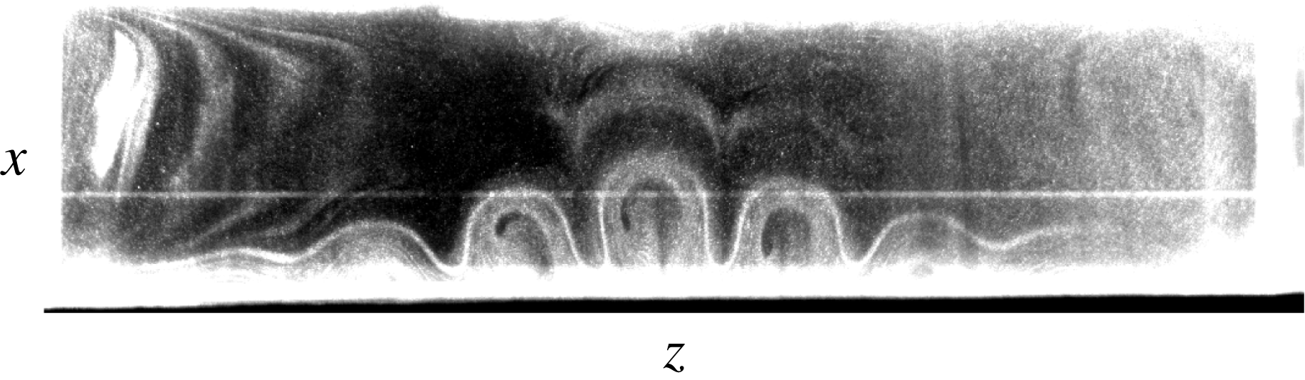
, by doubling the cavity depth. The investigated aspect ratios are gathered in table 2. Figure 19 shows how the amplitude of the structure is affected by the walls. The span is not large enough to allow the vortices to reach their saturated amplitude over a significant spatial range of the span (only reached midspan in figure 19). Instead, a monotonic ramp of amplitude from the end walls up to the centre of the cavity is observed.
The change in
 $S/D$
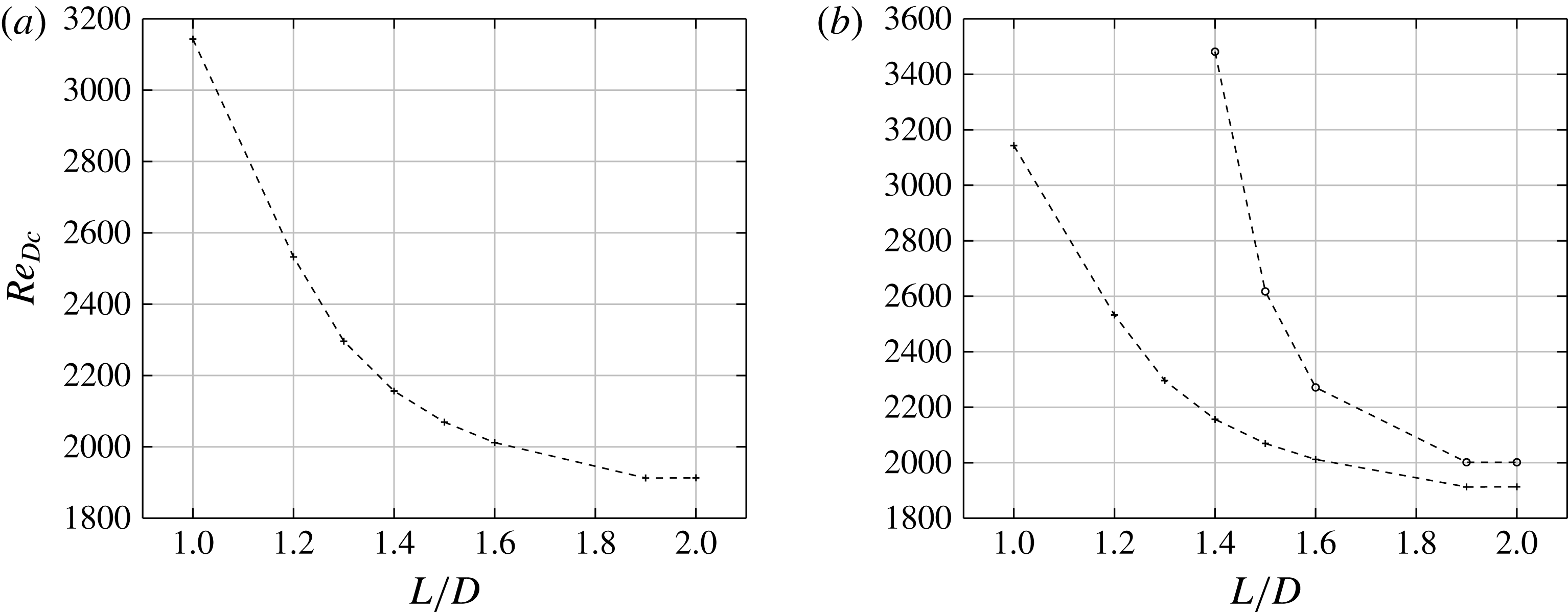
does not change the supercriticality of the bifurcation. Figure 20 shows the critical Reynolds number as a function of
 $L/D$
. The critical Reynolds number decreases monotonically when increasing
 $L/D$
, reaching an asymptotic value of approximately
 $Re_{D_{\infty }}=1900$
beyond
 $L/D=1.6$
, only slightly larger than the value found for
 $S/D=12$
.
Bifurcation thresholds for
 $S/D=6$
: (a) critical Reynolds number as a function of
 $L/D$
, determined from LDV measurement (observation time
 $120~\text{s}$
), (b) threshold of occurrence of the family of oscillatory mode as a function of the aspect ratio (○). The threshold of the primary bifurcation is also shown for comparison (
 $+$
).

Evolution of the Strouhal number associated with the primary pattern with the Reynolds number and aspect ratio
 $L/D$
for
 $S/D=6$
. The data scattering results is here the trace of the spectral resolution.

Wavelength evolution with
 $L/D$
for
 $S/D=6$
at
 ${\it\epsilon}=0.049$
for
 $L/D=1$
,
 ${\it\epsilon}=0.047$
for
 $L/D=1.2$
,
 ${\it\epsilon}=0.039$
for
 $L/D=1.3$
,
 ${\it\epsilon}=0.053$
for
 $L/D=1.4$
,
 ${\it\epsilon}=0.042$
for
 $L/D=1.5$
,
 ${\it\epsilon}=0.057$
for
 $L/D=1.6$
,
 ${\it\epsilon}=0.016$
for
 $L/D=1.9$
and
 ${\it\epsilon}=0.015$
for
 $L/D=2$
.

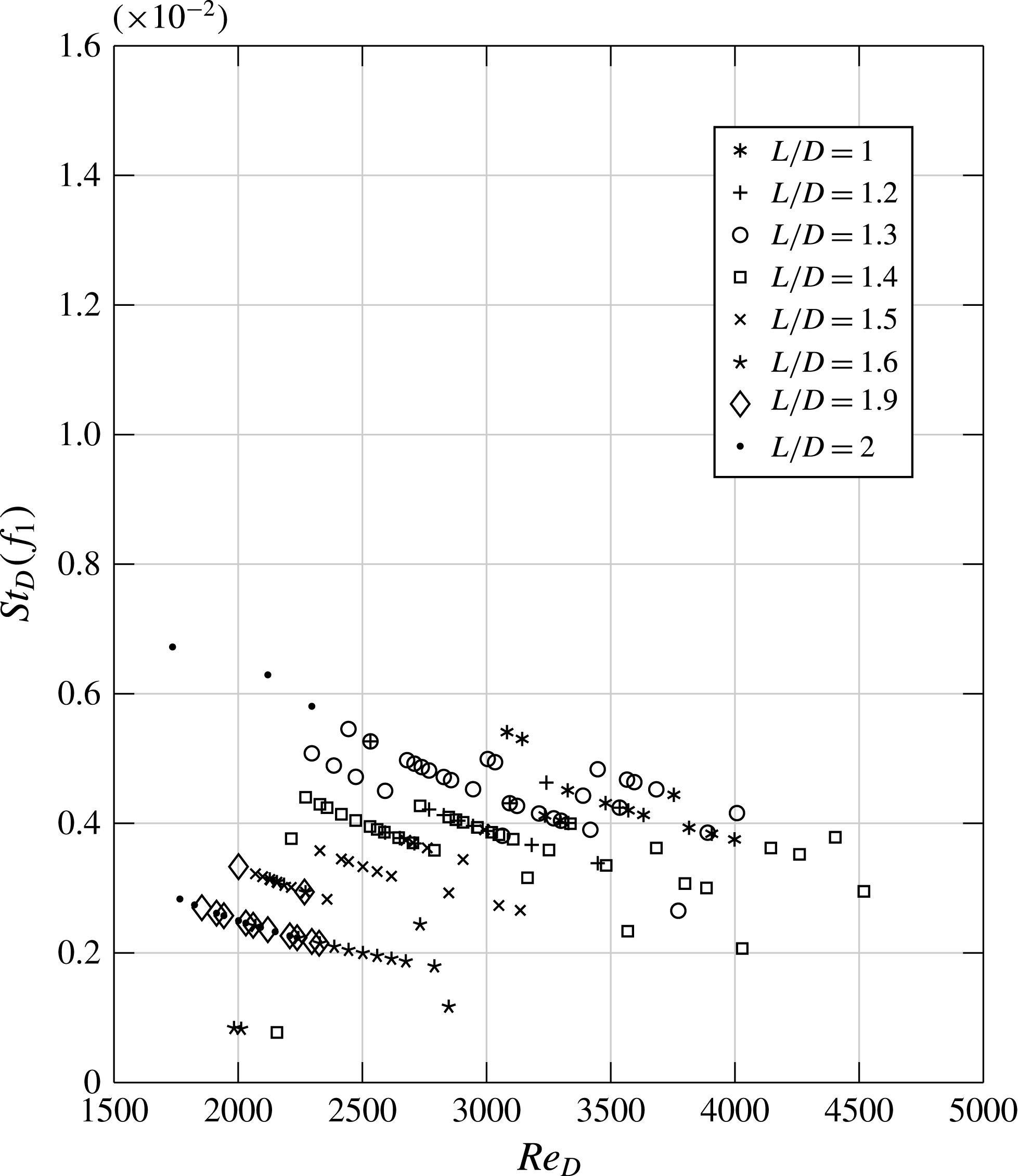
The evolution of the Strouhal number
 $St_{D}(f_{1})$
with the Reynolds number for several
 $L/D$
is presented in figure 21. Different from what was reported for
 $S/D=12$
, Strouhal numbers are now between
 $0.002$
and
 $0.006$
for any
 $L/D$
. Such values are typical of the Strouhal numbers found for the drifting steady modes identified in the configuration
 $S/D=12$
for small
 $L/D$
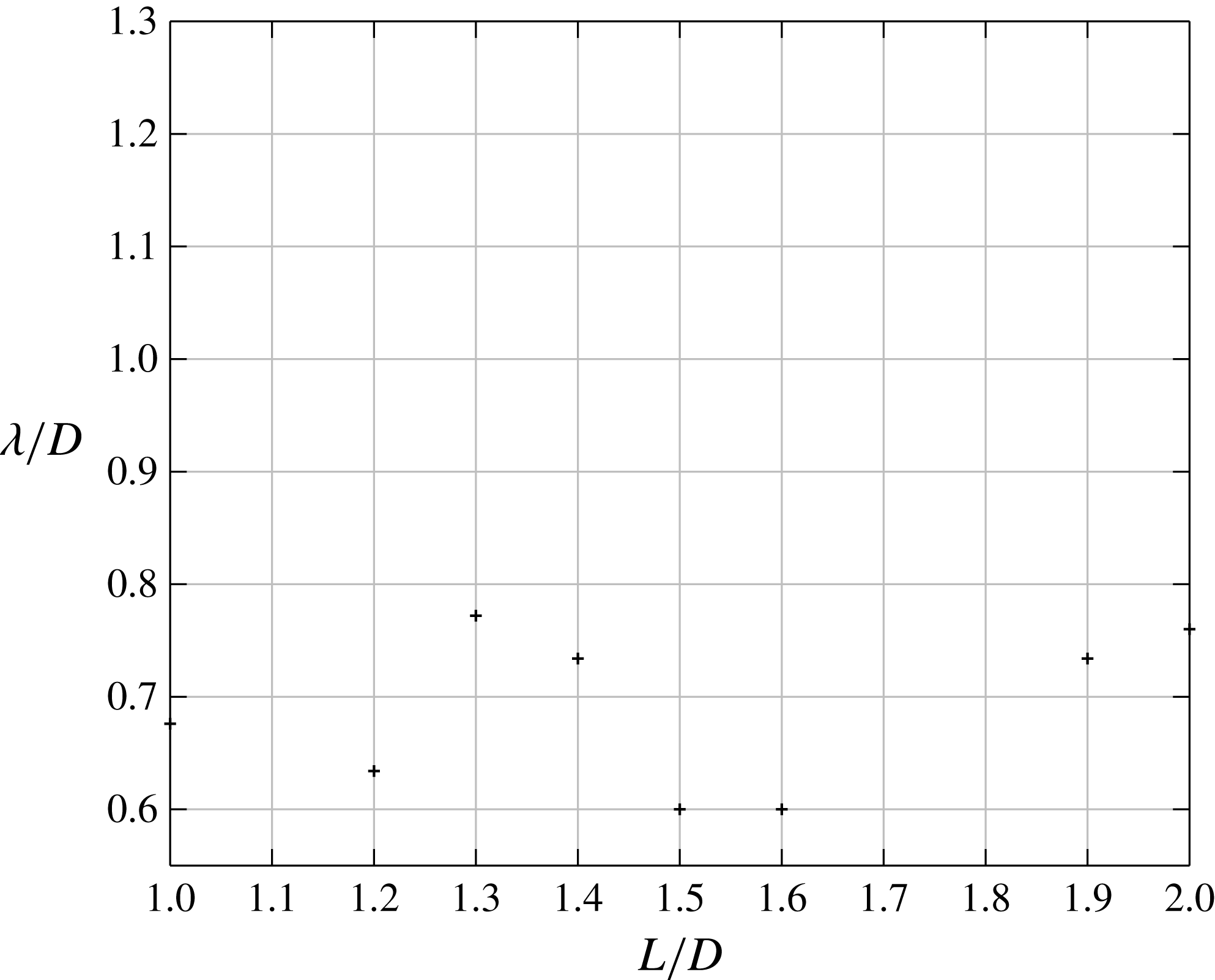
. The same is true for the wavelength of the structures, which are found to be between
 ${\it\lambda}/D=0.6$
and
 ${\it\lambda}/D=0.77$
for all
 $L/D$
, see figure 22. Therefore, only modes of the steady family are selected. The main consequence of an increase in the spanwise confinement is therefore to enhance the family of steady modes in cavities of large aspect ratio. This is in agreement with Faure et al. (Reference Faure, Pastur, Lusseyran, Fraigneau and Bisch2009), who identified Strouhal numbers, at Reynolds numbers between
 $4000$
and
 $5000$
, of the order of 0.007, typical of quasisteady modes, in a square open cavity with
 $S/D=3$
.
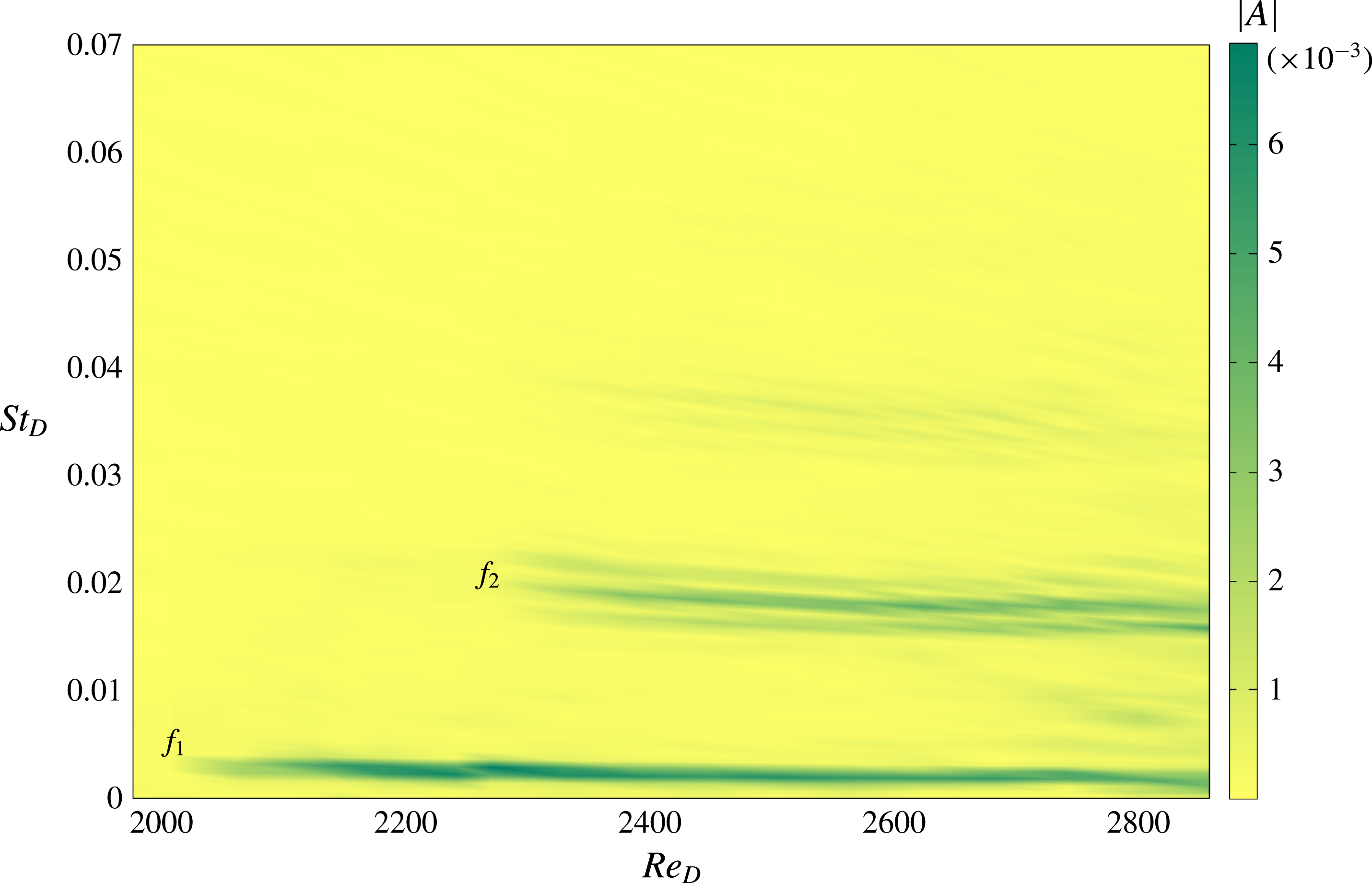
Bifurcation diagram based on the power spectral density (colour), for
 $S/D=6\;L/D=1.6$
.

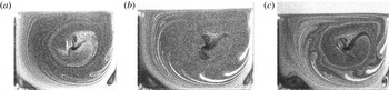
Smoke visualisations in a vertical plane: (a)
 $L/D=1.3\;Re_{D}=2335$
,(b)
 $L/D=1.4\;Re_{D}=2165$
, (c)
 $L/D=1.5\;Re_{D}=2065$
for
 $z/D=1.82$
.

This result is different from what was observed in confined lid-driven cavities. Aidun, Triantafillopoulos & Benson (Reference Aidun, Triantafillopoulos and Benson1991) indeed reported oscillatory structures for spanwise aspect ratio
 $S/D=3$
(strong confinement). When the confinement is relaxed, steady modes are observed in the core of the cavity, while propagating modes survive close to the sidewalls (Albensoeder et al.
Reference Albensoeder, Kuhlmann and Rath2001).
As shown in the spectrogram of figure 23, a propagating mode may also emerge in the power spectrum at larger Reynolds numbers, and coexist, in space and time, with the primary drifting steady mode. This, however, occurs only for cavities of large aspect ratio (
 $L/D\geqslant 1.4$
), when the secondary vortex, close to the upstream wall, is no longer confined to the bottom corner of the cavity, as shown in figure 24. The threshold of occurrence of the second mode is shown in figure 20(b).
4.3. Discussion with respect to other flows
All the results reported in the previous section are in good agreement with the predictions of recent linear stability analyses by Meseguer-Garrido et al. (Reference Meseguer-Garrido, de Vicente, Valero and Theofilis2011, Reference Meseguer-Garrido, de Vicente, Valero and Theofilis2014). In analysing the stability of the two-dimensional steady base flow with respect to spanwise perturbations, these authors showed that the mode with the largest growth rate belongs to a family of steady modes for aspect ratios
 $1\leqslant L/D\leqslant 1.2$
, whereas for
 $1.3\leqslant L/D\leqslant 3$
the most amplified mode belongs to a family of propagating modes, with wavelengths approximately twice as large as the wavelength of the steady family mode. In the compressible regime, Brès & Colonius (Reference Brès and Colonius2008) also identified steady critical modes for square cavities (
 $L/D=1$
), with wavelengths in the range
 $0.2<{\it\lambda}/D<0.6$
, whereas for cavities of aspect ratios
 $L/D=2$
and
 $4$
, the critical mode is oscillatory with wavelengths in the range
 $0.6<{\it\lambda}/D<1.4$
.
The change of family with respect to the aspect ratio was also observed in other flows undergoing centrifugal instabilities. This is, for instance, the case with lid-driven cavity flows. In particular, Albensoeder et al. (Reference Albensoeder, Kuhlmann and Rath2001) showed that the critical mode in square cavities is steady, whereas for larger aspect ratio the critical mode is oscillatory. In such flows, bifurcations are also reported to be supercritical (Albensoeder et al. Reference Albensoeder, Kuhlmann and Rath2001; Theofilis et al. Reference Theofilis, Duck and Owen2004).
The influence of the geometry on the mode selected by the flow in confined configurations is also found for backward-facing-step flows, where three-dimensional structures were observed, (Barkley, Gomes & Henderson Reference Barkley, Gomes and Henderson2002; Beaudoin et al.
Reference Beaudoin, Cadot, Aider and Wesfreid2004; Lanzerstorfer & Kuhlmann Reference Lanzerstorfer and Kuhlmann2012). In Lanzerstorfer & Kuhlmann (Reference Lanzerstorfer and Kuhlmann2012), it has been shown that, owing to the aspect ratio
 ${\it\Gamma}$
, defined as the ratio of the step depth over the total height of the canal, the three-dimensional structures are either stationary (small
 ${\it\Gamma}$
) or oscillatory (larger
 ${\it\Gamma}$
). In addition, this change of mode is correlated with a monotonic decrease of the critical Reynolds number with the aspect ratio
 ${\it\Gamma}$
.
5. Beyond the first steps of the instability
Evolution of the power spectral density (b,d,f,h) with the Reynolds number for
 $S/D=12$
and
 $L/D=1.75$
, from LDV measurement (a,c,e,g) in
 $x/L=0.386$
,
 $y/D=-0.88$
and
 $z/S=0.005$
. (a,b)
 $Re_{D}=1825$
; (c,d)
 $Re_{D}=1873$
; (e,f)
 $Re_{D}=1975$
; (g,h)
 $Re_{D}=2320$
.

Power spectral density evolution with Reynolds number for
 $S/D=12$
and
 $L/D=1.75$
of
 $f_{1}$
under increasing (
 $+$
) and decreasing (○) ramps of the velocity;
 $f_{2}$
under increasing (*) and decreasing (▵) ramps;
 $f_{-}$
under increasing (▫) and decreasing (♢) ramps. See text for details about
 $f_{1}$
,
 $f_{2}$
and
 $f_{-}$
.

Space–time diagrams built from a line of adimensional vorticity at
 $y/D=-0.30$
for
 $S/D=12$
,
 $L/D=1.75$
. Sampling frequency
 $f_{e}=15~\text{Hz}$
and number of snapshots
 $N_{cp}=1000$
. (a)
 $Re_{D}=2225$
, (b)
 $Re_{D}=2700$
, (c)
 $Re_{D}=3000$
, (d)
 $Re_{D}=5570$
.

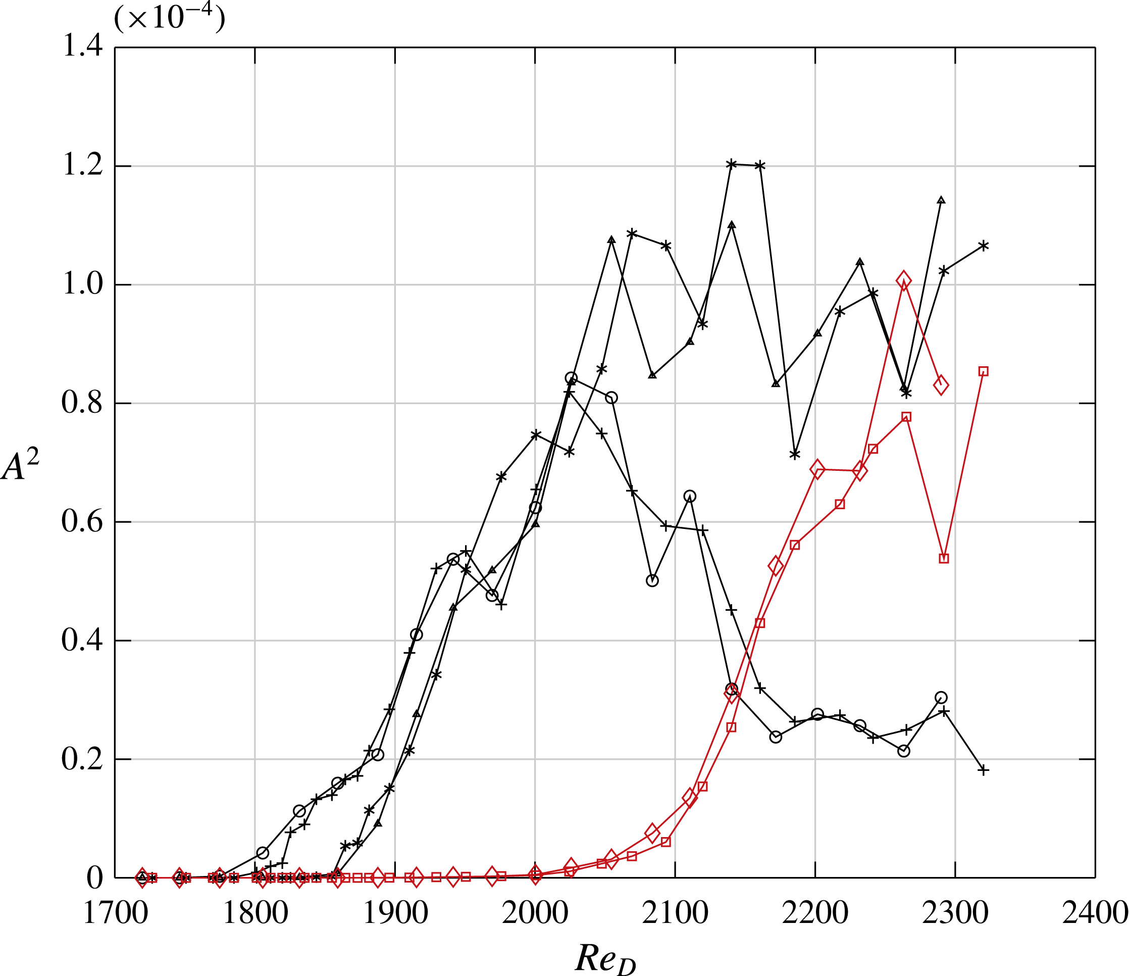
As expected, new peaks emerge in the power spectrum as the Reynolds number increases, as shown in figure 25. The first frequency to appear is the nonlinear combination
 $f_{-}=f_{2}-f_{1}$
, associated with the dynamic mode
 ${\it\psi}_{-}(x,z)$
, which is energetic where
 ${\it\psi}_{1}$
and
 ${\it\psi}_{2}$
are also energetic, and whose wavenumber obeys the resonant condition
 $k_{-}=k_{2}-k_{1}\simeq 2k_{1}$
. This result suggests that the main mechanism of energy transfer is a three-wave interaction process.
When a new mode emerges in the power spectrum, the amplitude evolution of the other modes breaks off, as illustrated in figure 26. However, as already mentioned, the seemingly erratic evolution of the amplitudes of
 $f_{1}$
and
 $f_{2}$
at larger Reynolds numbers is in fact mainly deterministic, as proved by the reproducible amplitude behaviour in both increasing and decreasing ramps of the control parameter.
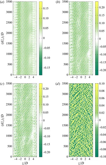
As new peaks emerge in the spectrum, the front dynamics at both sides of the wavepacket, as well as the dynamics of singularities in the amplitude of the wavepacket, become non-trivial, as shown by the space–time diagrams of figure 27 for four values of the Reynolds number. In figure 27(b), for instance (
 $Re_{D}=2700$
), the source between the left- and right-travelling waves, well characterised by its associated vanishing amplitude in the wave pattern, drifts slowly to the right-hand side of the cavity, disappears and emerges again in its initial position, cyclically in time.
At larger values of the Reynolds number, in addition to the source motion, the overlapping of the two travelling waves becomes intermittent in time. For instance, at
 $Re_{D}=3000$
(see figure 27
c), the overlapping pattern is present in the middle part of the cavity until
 $t\,D/U_{e}=500$
, after which both travelling waves no longer overlap and are separated by a source. Starting from
 $t\,D/U_{e}=1000$
, the interpenetrating pattern is recovered (the source has been convected out), and so forth repeatedly in time.
At the largest values of the Reynolds number, localised areas of coherent structures, though still identifiable in space and time, now coexist with areas where the dynamics is unstructured, as shown in figure 27(d) for
 $Re_{D}=5570$
. Such a regime was identified in Faure et al. (Reference Faure, Pastur, Lusseyran, Fraigneau and Bisch2009) as a so-called ‘turbulent’ regime. Note that, for this regime, as well as for
 $Re_{D}=3000$
, the shear-layer self-oscillations couple to the inner-flow dynamics, as shown in Basley et al. (Reference Basley, Pastur, Lusseyran, Soria and Delprat2014). The fine details of the route to space–time chaos in this system would require a study of its own, which is beyond the scope of this paper.
6. Conclusion
We performed a parametric experimental study of the three-dimensional structures inside an open cavity flow resulting from centrifugal instabilities. We highlighted a change in the mode selected by the flow at the threshold of the instability when the aspect ratio
 $L/D$
of the cavity is varied. Their features are in good agreement with predictions from linear stability analyses, which predict that the critical mode for cavities of small aspect ratio belong to the family of steady modes, whereas propagating modes are selected for larger aspect ratios. We identified the bifurcation threshold and showed that it corresponds to an imperfect supercritical fork bifurcation for small aspect ratio, and a Hopf bifurcation for larger aspect ratio, with a co-dimension two point at approximately
 $L/D=1.4$
. The base flow, in rectangular cavities, is more unstable against centrifugal instabilities than in square cavities. Experimentally, the vortical structures are always observed as drifting towards the sidewalls. Though very slow for cavities of small aspect ratio, the drift never vanishes, due to secondary flows that carry the vortical pattern. This is in agreement with the study of sidewall effects in Faure et al. (Reference Faure, Pastur, Lusseyran, Fraigneau and Bisch2009). Finally, we determined the effect of spanwise confinement by doubling the cavity depth. As a consequence, the propagating family of modes is no longer selected at threshold.
The centrifugal instabilities of the inner flow described in this paper generate a very weak velocity field, two orders of magnitude smaller than the incoming velocity. Despite this fact, considering their decisive impact upon the amplitude modulation of the self-sustained oscillations of the flow, as was shown in Brès & Colonius (Reference Brès and Colonius2008), Basley et al. (Reference Basley, Pastur, Lusseyran, Soria and Delprat2014), these centrifugal instabilities can arise as the determining effects behind the disturbing consequences of cavities, for instance in transport.
These characteristics, identified in an open cavity flow, are also found for lid-driven cavities and backward-facing steps, indicating that this simple geometry is the origin of generic phenomena. We believe that the results obtained from our analysis will be useful for a better understanding of confined recirculation flows.
Acknowledgements
This work was supported by CNRS, the Direction Générale de l’Armement (DGA) and ANR-12-BS09-0024-03 CoolJazz contract. P. Manneville is warmly acknowledged for his helpful comments. The authors would also like to kindly acknowledge J. Basley for fruitful discussions on this work.
Supplementary movies
Supplementary movies are available at http://dx.doi.org/10.1017/jfm.2015.726.