II. GO–PO COMBINATION METHOD AND ISAR IMAGING

A) Principle of GO–PO

The basic idea of GO–PO to calculate a target's RCS is described in the following. First of all, the target model is approximated by small triangle patches whether illuminated or not. When incident EM wave illuminates a surface element, the reflection direction can be determined according to GO. Let the ray do the intersection test with patches which satisfy the condition $\hat{n} \cdot \hat{i} \lt 0$ , for that only these patches can possibly be illuminated by incident wave, where $\hat i$ is the unit vector of the incidence wave; $\hat n$ is the unit normal of the patch.

In this method, the square root of RCS consists of three components, described as [Reference Wei and Zhang20]

(1) $$\eqalign{\sqrt \sigma = & \sum\nolimits_0 {i\displaystyle{k \over {\sqrt \pi}} \int_{s_m} {\hat e_r \cdot [\hat s \times (\hat n_m \times \hat h_i )]\exp (ik\vec r \cdot (\hat i - \hat s))ds_m}} \cr & + \sum\nolimits_1 {i\displaystyle{k \over {\sqrt \pi}} \int_{s_m} {\hat e_r \cdot [\hat s \times (\hat n_m \times \hat h_{r1m} )]}} \cr & \quad \exp (ik\vec r \cdot (\hat i_{r1m} - \hat s))ds_m \cr & \quad + \sum\nolimits_2 {i\displaystyle{k \over {\sqrt \pi}} \int_{s_m} {\hat e_r \cdot [\hat s \times (\hat n_m \times \hat h_{r2m} )]}} \cr & \quad \exp (ik\vec r \cdot (\hat i_{r2m} - \hat s))ds_m,}$$

where the $\Sigma_0, \,\Sigma_1, $ and $\Sigma _2$ are operated on the patches illuminated by the incident field, first reflected field, and second reflected field, respectively; $\hat e_r$ is the unit vector of electric polarization of far-field receiver; $\hat s$ is the unit vector of scattering wave; $\hat n_m$ is the unit normal of the m-th patch; $\hat h_i$ is a unit intensity vector of the incident magnetic field; $\hat h_{r1m}$ and ${\hat h}_{r2m}$ are the magnitude vectors of the first reflected and second reflected magnetic field illuminating on the m-th patch, respectively; $\hat i$ is the unit vector of incidence wave; $\hat i_{r1m} $ and $\hat i_{r2m} $ are the unit vectors along the direction of the first reflected and second reflected magnetic field illuminating on the m-th patch, respectively; s _m in the integral represents the surface of the m-th patch. Otherwise, the polygon integration over each patch can be easily converted into a contour integration with Gordon method. Take the m-th patch, for example [Reference Gorden21]

(2) $$\eqalign{&{i\displaystyle{k \over {\sqrt \pi}} \int_{s_m} {\hat e_r \cdot [\hat s \times (\hat n_m \times \hat h_i )]e^{ik\vec r \cdot (\hat i - \hat s)} ds_m}} \cr & \quad = \displaystyle{{\hat e_r \cdot [\hat s \times (\hat n_m \times \hat h_i )]} \over {\sqrt \pi T}}e^{ik\vec r_0 \cdot \vec \omega} \cr & \qquad \times {\sum\limits_{m = 1}^M {(\hat p\!\cdot\!\vec a_m )e^{ik\vec r_m \cdot \vec \omega}} \displaystyle{{\sin (k\vec a_m \cdot \vec \omega /2)} \over {k\vec a_m \cdot \vec \omega /2}}},}$$

where ${\mathop{r}\limits^{\rightharpoonup}}_0 $ is the position vector of an origin on or near the patch; $\hat p = \hat n \times {\mathop{\omega}\limits^{\rightharpoonup}}/\hat n \times {\mathop{\omega}\limits^{\rightharpoonup}} $ is a unit vector in the plane of the patch perpendicular to ${\mathop{\omega}\limits^{\rightharpoonup}}, {\mathop{\omega}\limits^{\rightharpoonup}} = \hat i - \hat s;$ T is the length of the projection of ${\mathop{\omega}\limits^{\rightharpoonup}} $ onto the plane of the patch; ${\mathop{a}\limits^{\rightharpoonup}} _m $ is a vector describing the length and orientation of the m-th edge of the patch, arranged tip to tail around the perimeter; ${\mathop{r}\limits^{\rightharpoonup}} _m $ is the position vector of the midpoint of the m-th edge; and M is the number of patch edges.

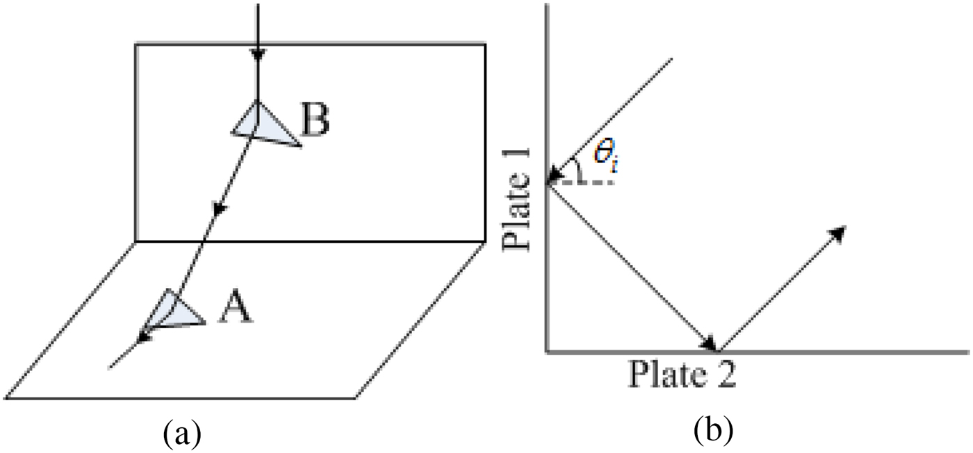
Taking the dihedral corner reflector, for example firstly, it is assumed that if the central ray reflected by patch A intersects the patch B, the entire patch B is illuminated by parallel rays reflected by patch A. As Fig. 1 shows, the reflector is a right-angle corner and both surfaces have been partitioned into small triangle patches. Incident rays reflected by plate 1 intersect the plate 2 in some area. In Fig. 1(b), for θ _i <45^o, the entire plate 2 is illuminated by the rays reflected from the bottom part of the plate 1. In this case, the number of the patches of the bottom part of the plate 1 is much less than that of the entire plate 2. If the normal central ray-tracing is still adopted, many patches of the plate 2 will be missed. For θ _i >45^o, many patches of the plate 2 will be traced repeatedly.

Fig. 1.

General view of a ray illumination on a dihedral corner reflector. (a) Front view. (b) Lateral view.

Accordingly, the backward ray-tracing is adopted for the identification. For a patch on the plate 2, the tests with the patches, which have been illuminated by the incident rays, are done one by one. In every test, there is one patch A from plate 2 and one patch B from the illuminated patches of the plate 1. We let the origin of the ray be the direction contrary to the one of the ray reflected by patch B. If the ray and the patch B intersect with each other, it is considerate that the patch A is illuminated by the reflected field of the patch B. Otherwise, the test moves onto the next illuminated patch. If all the rays do not intersect the patches respectively, the patch A can be thought not illuminated by the reflected field. If the target structure is relatively complex, we must make sure that the ray is not cut by other patches between the patch A and patch B before the positive identification.

As for the computation about the second reflected field, the only thing need to do is to replace the patches illuminated by the incident wave by the ones illuminated by first reflected field, and the other parts of the algorithm are absolutely the same with the one for the first reflected field.

B) Verification of GO–PO algorithm

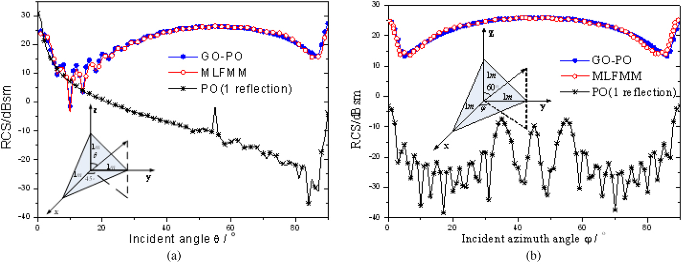
As we all know, the trihedral corner reflector is a typical benchmark target for the verification of high-frequency multiple-bounce scattering. The method above is applied to study the backscattering characteristic of a trihedral corner reflector, as is shown in Fig. 2, which is compared with MLFMM in FEKO as well as pure PO method for only first reflection considered. The trihedral corner reflector used in this paper is constructed of three right-angled triangles with the side length of 1 m.

Fig. 2.

Backscattering RCS comparison between GO–PO, MLFMM, and pure PO method for a trihedral corner reflector. (a) VV polarization for φ = 45° at 3.0 GHz. (b) HH polarization for θ = 60° at 6.0 GHz.

The results show a great agreement between the combination method GO–PO result and the MLFMM result for both VV and HH polarizations at different frequencies, which proves the effectiveness and accuracy of the GO–PO method. The significant difference between GO–PO or MLFMM results and PO results indicates the dominant effect of multiple reflections on the scattering characteristic for such a corner reflector. The comparison of the computation time of two methods is illustrated in Table 1, which is the total time cost for all the 90 incidence angles. It is worth to notice that the GO–PO method appears to be much more efficient than MLFMM, especially in the high-frequency case.

Table 1.

Comparison of the computation time of different methods.

III. ISAR IMAGING OF MOVING SATELLITE

ISAR generally refers to the case where the radar platform stays stationary while the target is moving. The motion of a target can be decomposed into the translational component and rotational component. It is assumed that there is a reference point usually located in the geometrical center of the target. The translational component refers to the movement of reference point along the track of moving target and the objective attitude relative to radar platform remains unchanged; the rotational component is that the target rotates around the reference point. When the target is represented by scatterers and is located in the far-field region of radar, the translational component has no influence on the radar echo Doppler. However, the translational component must be compensated in the imaging processing.

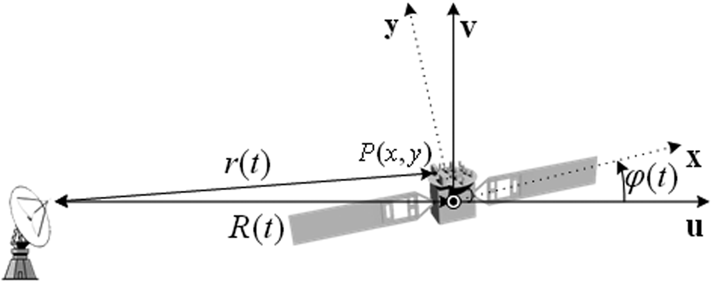
Assuming that the satellite moves along the radar line of sight (RLOS) axis, u, and rotates around its main axis, as Fig. 3 shows. The received signal can be theoretically approximated as an integration of the backscattered echoes from all scatterers inside the radar beam [Reference Chen and Ling18]

(3) $$g(t) = \int {\int_{ - \infty} ^\infty {A(x,y)\exp \left( { - j4\pi f\displaystyle{{r(t)} \over c}} \right)dxdy}}, $$

where A(x, y) is the backscattered field amplitude of a point scatterer. For a target located at the far field relative to the radar, the distance from a point P to the radar can be expressed as

(4) $$r\left( t \right) \cong R(t) + x\cos \varphi (t) - y\sin \varphi (t),$$

where R(t) means the target's translational range off the radar and φ(t) represents the rotational angle with respect to the RLOS. Then, the exponential term in equation (3) can be expanded into φ ^t and φ ^r that relate to the translational motion and the rotational motion, respectively.

(5) $$\eqalign{& \varphi ^t = \exp \left\{ { - j4\pi \displaystyle{f \over c}\left( {R_0 + v_t t + \displaystyle{1 \over 2}a_t t^2} \right)} \right\}, \cr & \varphi ^r = \exp \left\{ { - j4\pi \displaystyle{f \over c}[x_p \cos (\varphi _0 + \omega _r t) - y_p \sin (\varphi _0 + \omega _r t)]} \right\},} $$

where R ₀ is the initial position of the satellite; v _t and a _t are translational velocity and acceleration, respectively. φ₀ is the initial angle and ω _r is the angular velocity of the satellite.

Fig. 3.

Geometry of moving satellite with respect to radar.

Considering the complicated target motions, the motion compensation (MOCOMP) technique must be applied to eliminate the undesired effects of motion on the ISAR image. Firstly, an estimation of the motion parameters is executed through the matching pursuit (MP) technique so as to compensate the radial motion errors [Reference Mallat and Zhang22–Reference Li, Zhang, Wang and Xia24]. The unknown translational motion parameters of v _t and a _t are estimated with an iterative search in a rough range of parameters by projecting the radar echoes on a 2D space. The estimated values $v_t^{est} $ and $a_t^{est} $ would be the parameters which give the largest projection

(6) $$A = {\max}_{(v_t, a_t)} \{ \langle g(t) \cdot \varphi ^t (v_t, a_t, t)\rangle \}, $$

where the inner product is defined as

(7) $$\langle g \cdot \varphi ^t \rangle = \int_{v_t} {\int_{a_t} {g(t) \cdot (\varphi ^t (v_t, a_t, t))^ * da_t dv_t}}. $$

Then, the translational motion errors can be mitigated by a phase correction to the original echoes as follows

(8) $$s(t) = g(t)\!\cdot\!\varphi ^t (v_t^{est}, a_t^{est}, t)^*. $$

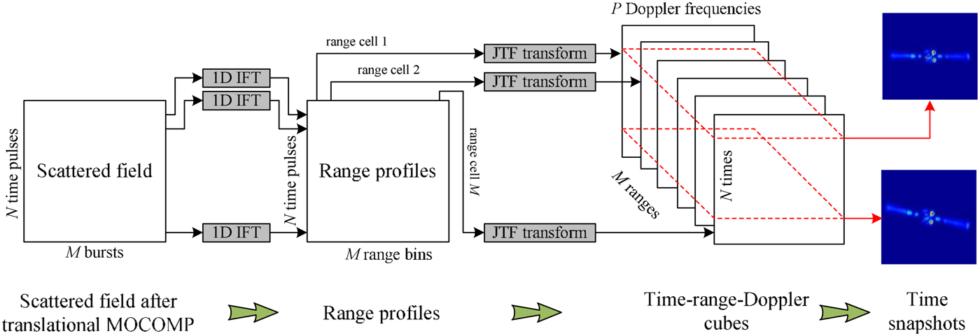
As for the rotational MOCOMP, the JTF transformation is applied to extract the instantaneous Doppler frequency information of the range-Doppler data so as to construct the snapshots of the time-varying ISAR image. The schematic algorithm is illustrated in Fig. 4. After translational MOCOMP to the scattered field, the 1D IFT (inverse Fourier transform) is firstly applied to obtain the range profiles. Based on this, an employment of JTF transformation is conducted to the pulses for every range cell, resulting in a time-range-Doppler cube of size M × N × P, which provides the range-Doppler image at a selected time instant. Finally, extraction of different slices from the cube corresponds to the instantaneous 2D ISAR image of the target while rotating.

Fig. 4.

Schematic representation of JTF method for the rotational MOCOMP.

IV. NUMERICAL RESULTS AND ANALYSIS

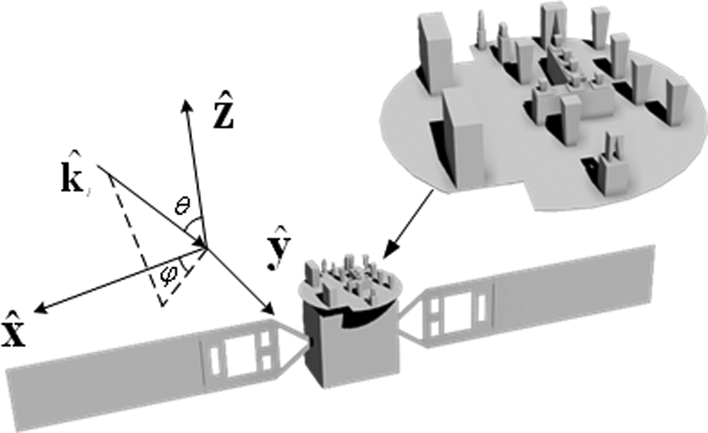
The GO–PO method is firstly used to analyze the EM scattering of a satellite model with complex antenna structures, which contains many corner structures, such as dihedral reflectors, as Fig. 5 shows. The model is 10.183 m long at the largest dimension and is partitioned into 46409 small patches. Here the model without antenna structure is partitioned into 31 084 small patches.

Fig. 5.

Geometry of the satellite model.

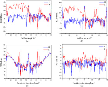
The comparisons of backscattering RCS results between the entire model and the model without antenna structure at 6.0 GHz for VV-polarization are shown in Fig. 6. In the following simulated results, the symbol N represents the model without antenna structure and E the entire satellite model. It can be seen obviously that the RCS for the complex satellite varies greatly with incident angle. The main reason is that the satellite model typically contains dozens of scatterers with significant contribution. The number of scatterers is so many that the contributions of all components to the RCS of the models are continuous either in phase or reverse phase, thus resulting in mutual interference, which leads to a heavy oscillation of the RCS curve. In Figs 6(a) and 6(b), it is illustrated that when in the XOZ plane, the entire antenna structure can be scanned in the range (0^o-90^o) of θ. Consequently, while removing the antenna structure, the RCS in the range (0^o-90^o) decreases about 20 dB. Moreover, for that the antenna cannot be illuminated in θ(90^o-180^o), the results of the two models show a slight difference. When in the XOY plane, as Fig. 6(c) shows, there are two peaks at 55° and 125° on the curve of the entire model for the multiple reflections, and both are about 20 dB larger than the RCS of the model without antenna. In the non-specific angles, as shown in Fig. 6(d), the RCS of entire satellite is larger than the other. Thus, the above analysis shows that the antenna structure is a strong scattering source. Furthermore, the multiple reflections among different structures and the corner reflectors could affect the scattering characteristic of a target greatly.

Fig. 6.

Backscattering characteristics of satellite under different incident angle. (a) φ = 0°. (b) φ = 180°. (c) θ = 90°.(d) θ = 30°.

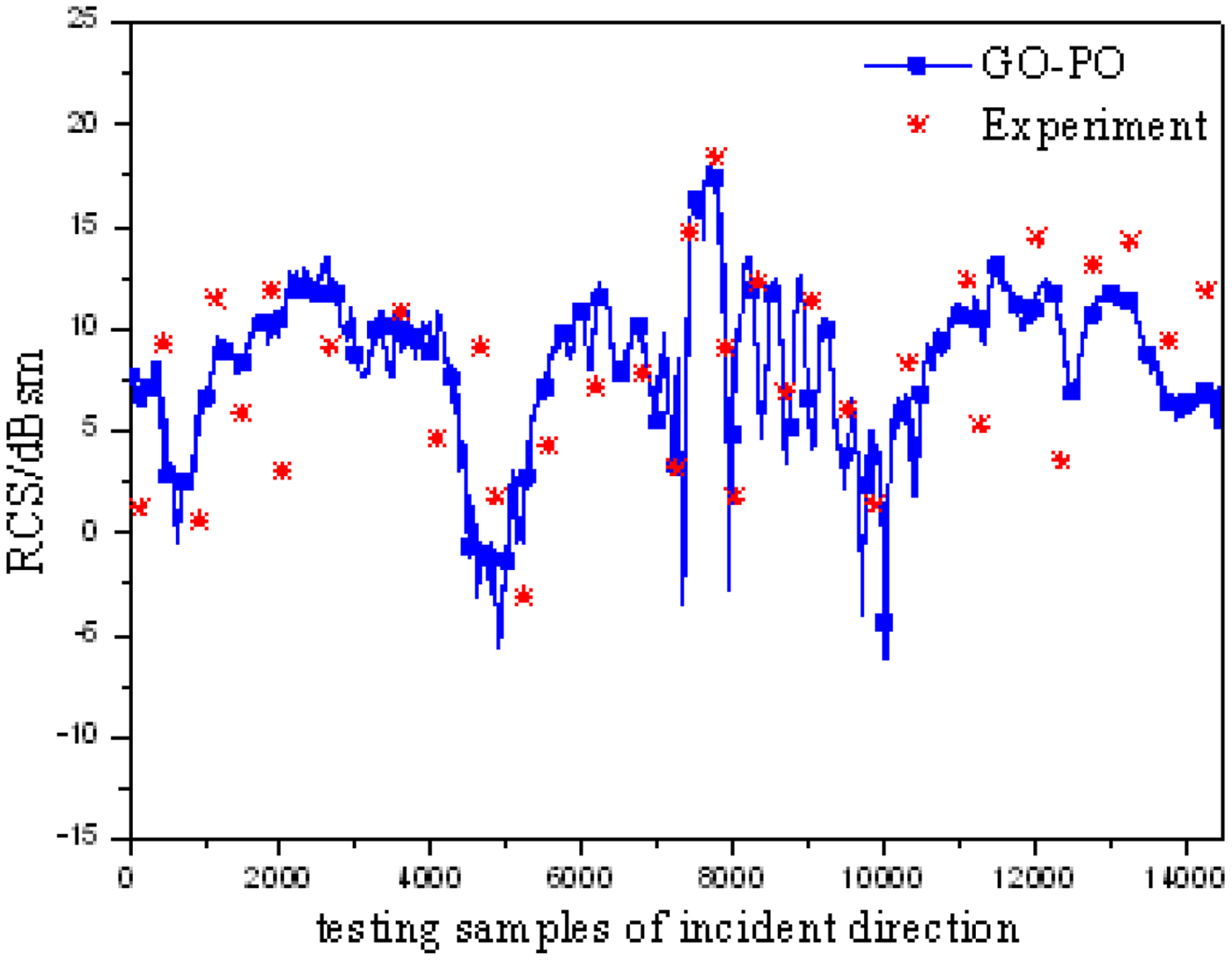
Figure 7 shows the comparison of GO–PO combination method result with the experimental result for RCS prediction of the entire satellite model at 3.0 GHz for VV-polarization. Notably, both the incident angel θ and φ in simulation are consistent with the experimental process. The abscissa is only noted with sample numbers. From the contrast, the GO–PO method considering the multiple reflections appears a good agreement with the experiments. Therefore, this combination method is verified with enough accuracy for scattering analysis of such complex targets.

Fig. 7.

Comparison of GO–PO result with experimental result for RCS prediction of satellite.

Since the simplicity and extensive application of range-Doppler method for ISAR imaging, it is first applied in the simple turntable model. In the simulations, the radar transmits stepped frequency signals at a central frequency 6.0 GHz with bandwidth 512 MHz, including M = 128 stepped frequencies in a burst and totally N = 128 bursts. The radar echoes are received from an incident angle $\theta = 45^{\rm o}$ and an azimuth angle $\varphi = 45^{\rm o}$ . 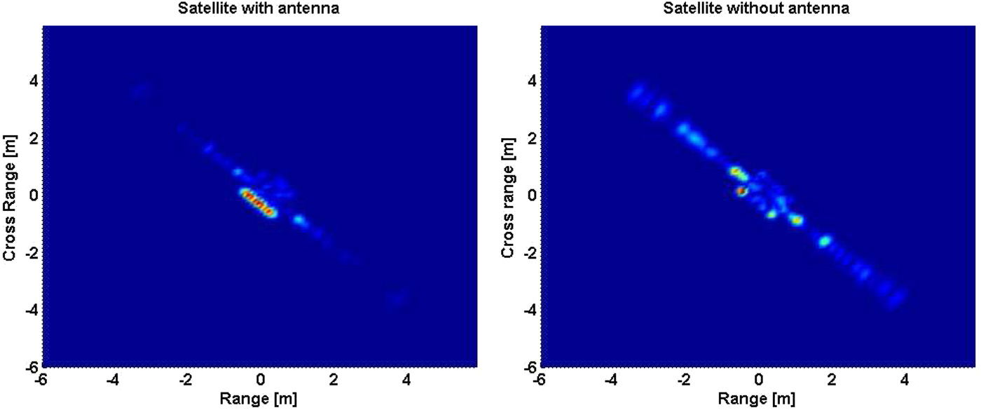The ISAR imaging results are shown in Figs 8(a) and 8(b) for satellite with and without antenna structure, respectively. The comparison between two images reflects that the antenna structure is almost the strongest scattering part and also weakens the effect of wing plate. This is owing to the fact that for a corner reflector, the maximum backscattering intensity always occurs near this incidence. However, the antenna on the satellite contains several reflectors, either dihedral or trihedral.

Fig. 8.

ISAR images for the satellite models with and without antenna. (a) Satellite with antenna. (b) Satellite without antenna.

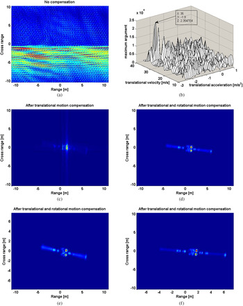
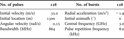
In the following simulations, assuming that the satellite with antenna has both translational and rotational movements, the motion parameters are listed in Table 2. The simulated results are shown in Fig. 9. However, without any compensation, see Fig. 9(a), the image is highly distorted, defocused, and blurred owing to high velocity in both radial and rotational directions. To compensate the translational motion, the MP search is used for the estimations of both translational velocity and acceleration. After the iterative search routine, the estimated values of $v_t^{est} = 35\;{\rm m/s}$ and $a_t^{est} = - 1.9\;{\rm m/}{\rm s}^{\rm 2}$ are successfully found in Fig. 9(b). Accordingly, the translational MOCOMP can be executed by employing equation (8) and the corresponding ISAR image is plotted in Fig. 9(c). The image clearly demonstrates the performance of the translational MOCOMP so that only the rotational motion-based defocusing remains in the ISAR image. For the compensation of rotational motion effects, the Gabor-wavelet transform using Gaussian blur function is employed as the JTF tool. The resultant image is clearly given in Fig. 9(d), in which the phase errors caused by translational and rotational motions of the satellite have been eliminated. Therefore, the motion-free ISAR image is very well focused and the strong scattering centers are well localized on the antenna.

Fig. 9.

ISAR images of moving satellite with antenna. (a) Conventional ISAR image (no compensation). (b) 2D MP search for translational parameters. (c) ISAR image (after translational MOCOMP). (d) ISAR image (after both MOCOMPs). (e) ISAR image (change angular velocity). (f) ISAR image (change bandwidth).

Table 2.

Radar and target parameters for imaging simulation.

What's more, the ISAR images of the satellite under different parameters are simulated. Considering that the translational motion effects are always compensated based on the estimated values, the angular velocity and the bandwidth variations are realized for comparisons. Firstly, the angular velocity is increased to ω _r  = 0.2 rad/s with other parameters invariant and the result is shown in Fig. 9(e). With an increase of angular velocity, the total azimuth angle of the satellite rotates is larger than that in Fig. 9(d) in the same imaging integrated time, thus resulting in an improvement to the cross-range resolution. Meanwhile, the contribution of the wing plate to the received echoes is increased owing to the wider azimuth angle. In addition, change the bandwidth to BW = 1264 MHz and remain other parameters unchanged. The final ISAR image is illustrated in Fig. 9(f). The range resolution would be improved with the increasing signal bandwidth, thus the structure of satellite becomes clearer in range direction than in the Fig. 9(d).

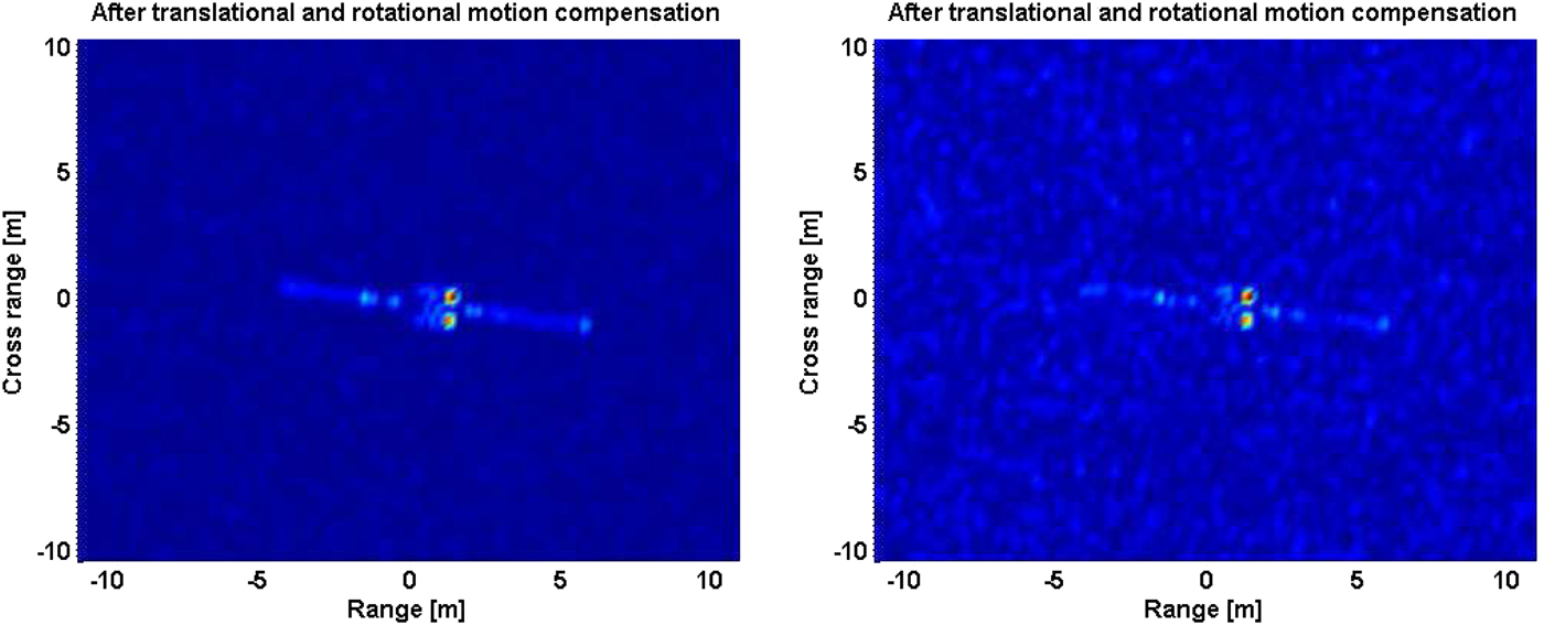
To discuss the noise influence on ISAR images, Fig. 10 shows the ISAR images of moving satellite with additive random noise. The noise signal is chosen to be white Gaussian with the signal-to-noise ratio (SNR) of −10 and −20 dB. The simulation parameters keep the same as that in Fig. 9(d). Under a relative high SNR in Fig. 10(a), the scatterers on the satellite are resolved well in the motion-free ISAR image. While decreasing the SNR to −20 dB in Fig. 10(b), the wing plate structure would be a little harder to distinguish. However, the antenna structure is still easily observed owing to the strong radar scattering.

Fig. 10.

ISAR images of moving satellite with additive random noise. (a) SNR = −10 dB. (b) SNR = −20 dB.

V. CONCLUSION

An efficient combination of GO and PO methods is proposed to study the EM scattering from electrically large and complex target with the consideration of multiple reflections. The model deals with the initial reflection using GO and the subsequent reflections are performed using PO. This could maintain the planar character of a wave upon reflection from a flat surface. In the ray-tracing part, the ray was traced backwards so that the contributions of some patches will not be missed or computed repeatedly. Numerical simulations are in excellent agreement with the measurements.

In the ISAR imaging simulation of the moving complex satellite, the radar echoes are collected at different frequencies and positions. The proposed GO–PO method is shown to be much more effective than the low-frequency numerical method. By applying the MOCOMP technique, the imaging results prove that the multiple reflections from antenna structure are dominant in the EM scattering of the complex satellite. Besides, the strong noise shows greater influence on the wing plate than the antenna structure in the ISAR images.