Introduction
The mortality of piglets within litter is caused by many factors. Individual birth weight is one explanatory variable for piglet survival (Knol et al., Reference Knol, Ducro, van Arendonk and van der Lende2002). Roehe and Kalm (Reference Roehe and Kalm2000) included individual birth weight and birth weight variation within litter as covariables in (generalized) linear mixed models to fit preweaning survival. Both effects were shown to be significant. Högberg and Rydhmer (Reference Högberg and Rydhmer2000) associated a higher litter size with a decreased survival rate. The authors argued that mortality was caused not only by low birth weights but also by higher weight variation within litter. They treated the standard deviation of birth weights within litter as a maternal trait and estimated a heritability of 10%. Damgaard et al. (Reference Damgaard, Rydhmer, Løvendahl and Grandinson2003) characterized genetic effects on sow productivity traits and analysed the within-litter variation in birth weight and the change in within-litter variation during suckling. The authors studied the standard deviation of birth weights of liveborn piglets and verified a heritability of 8% of this maternal trait. They found positive genetic correlations between within-litter variance and proportion of dead piglets at birth and during suckling. Thus, high variability of birth weight has a negative influence on sow productivity. Similar results were found by Huby et al. (2003). The authors concluded that, from a genetical perspective, survival is linked more closely to homogeneity of birth weights within litter than to mean birth weight.
Uniformity of body weight and growth is desirable not only at birth but also in later ages, since it allows for slaughtering at nearly the same age and makes management of fattening pigs easier. Several studies compared the further development of piglets of low, medium and heavy birth weight (most recently Rehfeldt et al., Reference Rehfeldt, Tuchscherer, Hartung and Kuhn2008; see also this article for further references). Significant differences for carcass composition, growth and meat quality were found at mature slaughter age. Hence, within-litter variability describes the starting point of litter growth and thus contributes to the final uniformity of carcasses.
The main issue of this article was to verify and estimate the importance of the genetic influence on the variability of birth weight within litter. In extension to previous studies, we consider the sex effect on piglet birth weight when analysing different measures of birth weight variability within litter. Furthermore, an impact of piglet’s sex on birth weight variability is assumed. Hence, as a first step, the sample variance of birth weights within litter separated by sex is assigned as a trait of the sow. Two transformations of the sample variance are analysed by a linear mixed model (LMM; Henderson, Reference Henderson1953). Furthermore, a generalized linear mixed model (GLMM; McCullagh and Nelder, Reference McCullagh and Nelder1989; Schall, Reference Schall1991) is applied to the untransformed sample variance within litter. The significance of the sex effect on birth weight variability is tested by an F-test with adjusted denominator degrees of freedom (Kenward and Roger, Reference Kenward and Roger1997). As a second step and in case of a non-significant sex effect on birth weight variability, we put forward the pooled sample variance of male and female birth weights within litter as a suitable measure of within-litter variance.
In addition, the presence of the random boar effects is verified by a likelihood ratio test. Variance components are estimated via REML (Patterson and Thompson, Reference Patterson and Thompson1971) and thereof heritability is estimated. The statistical models are evaluated with respect to appropriateness in terms of residual behaviour.
In future, the results of this study may be applied in practical breeding or in organizing selection experiments in order to reduce the variability of birth weight within litter and to increase piglet survival or, at least, to keep it constant.
Material and methods
Data
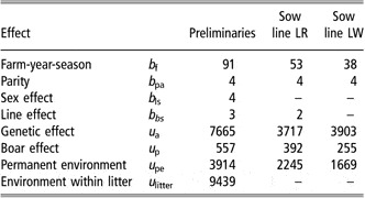
The dataset was provided by the German breeding organization Bundeshybridzuchtprogramm (BHZP). In total, the data consisted of 103 266 birth weights of 9439 litters of Landrace (line LR, 5379 litters) and Large White (line LW, 4060 litters) of a period from January 2002 to August 2006. In total, N = 3914 sows (line LR: 2245; line LW: 1669) with observations were considered. They were mated to 557 boars (line LR: 257; line LW: 300). The corresponding pedigree included 7665 animals of up to 10 generations backwards. Most of the litters were purebred, but 1134 litters arose from a cross of boar line LW and sow line LR. Boar line LR and sow line LW crossbred piglets did not appear. Only piglets born alive were weighed and included for further investigations. The average litter size was  (11.2) in sow line LR (sow line LW). Most births were observed up to the third parity (40.7%, 26.6% and 16.6%). The average birth weight of male and female progeny and its standard deviations are listed in Table 1. This list shows that birth weight of male piglets was in average heavier but also more variable than birth weight of females. Moreover, purebred piglets were somewhat lighter than crossbreds and less variable in birth weight. The data were collected from five farms, where three farms bred sow line LR and two farms bred sow line LW exclusively.
Comparison of birth weights (measured in grams) depending on pig line

Preliminary statistical models
From the literature (e.g. Bereskin et al., Reference Bereskin, Shelby and Cox1973; Arango et al., Reference Arango, Misztal, Tsuruta, Culbertson, Holl and Herring2006) it is known that piglet’s sex affects its birth weight. Thus, we have to consider the difference in mean birth weight of male and female piglets. We additionally assume that a sex effect on the variability of birth weight within litter exists. This effect is included in the preliminary statistical models and its significance is tested afterwards. Piglet birth weights are assumed to be independently and normally distributed within litter. The resulting trait per sow i in parity p is the sample variance  of birth weights within litter separated by sex g. Thus, usually two observations are counted per litter: one for male (g = 1) and one for female piglets (g = 2). Let
 denote the vector of sample variances ordered successively by sow i∈{1,…,N}, parity p∈{1,2,…} and sex g∈{1,2} and n is the total number of observations. The vector m = (m 1,…,mn)′ contains the number of piglets born per sow, parity and sex corresponding to the order of S 2. The sample variance
 of independently and normally distributed birth weights is proportional to a χ 2-distributed random variable with (mj−1) degrees of freedom, j = 1,…,n. Note that a χ 2-distribution is related to a gamma distribution. Two transformations are apparent to achieve an approximately normally distributed response. First, the distribution of the sample standard deviation
 is well approximated by a normal distribution (Fisher, Reference Fisher1922; Johnson and Kotz, Reference Johnson and Kotz1970). Furthermore, the distribution of
 is asymptotical normal (Box and Cox, Reference Box and Cox1964; Johnson and Kotz, Reference Johnson and Kotz1970).
Linear mixed models (LMM)
Now the presented measures of birth weight variability are fitted by an LMM. The elements of the response vector (Y 1,…,Yn)′ refer to one specific transformation of the sample variances, meaning the elements of Y are either the sample standard deviations or the logarithmized sample variances. The trait is modelled by

This model consists of the vector of fixed effects β′ = (b f,b pa,b ls,b bs), the vector of random effects u′ = (u a,u p,u pe,u litter) and the vector of residual deviations e.
β summarizes the effects of farm-year-season b f (four seasons per year), parity of sow b pa (1, 2, 3, ⩾4), sex effect b ls differing between sow lines and line effect b bs that takes into account crossbreeding effects. The random effects are the sow’s genetic effect  with use of the numerator relationship matrix A, the permanent environment
 affecting all litters of one sow, the permanent environment within one litter
 and the effect of boar (father of litter)
 . The latter accounts for the effect of boar heterozygosity on within-litter variability. The X and Z are known incidence matrices for the fixed and random effects, respectively. Number of levels of fixed and random effects are listed in Table 2.
Levels of fixed and random effects

First column: preliminary joint analysis of all data; second and third column: separate analyses of line LR and line LW data.
The residuals e~N(0,R) are normally distributed with the covariance matrix  . The matrix W represents a diagonal matrix of weights depending on the investigated response variable. The individual weight is concluded from the reciprocal of the conditional variance Var(Yj|u), which is approximated by a Taylor expansion of first order. For the trait
 constant weights are given by

The conditional variance of the trait Yj = Sj given the random effects u includes the conditional expectation E(Sj|u), which is indeed unknown. Thus, we apply a prediction of the sample variance  and achieve the weight

The trait Sj is special in that the vector of weights w is iteratively updated by the latest predicted standard deviations within litter separated by sex to improve parameter estimates. The iterations stop when convergence is reached and in case of leastwise 10 iterations have been performed. The convergence criterion is met when ||w (k+1)−w (k)|| < 10−6, where w (k) represents the vector of weights in the kth iteration.
It is assumed that residuals e and random effects u are independently distributed. Hence, the response Y is multivariate normally distributed with the covariance matrix

To compare our results with the literature we additionally analyse the sample standard deviation  per sow, parity and sex via model (1) without weights, then it is
 .
Generalized linear mixed model (GLMM)
In contrast to the investigations above, the untransformed response vector S 2 may directly be fitted by a GLMM. To distend, we introduce a multiplicative model with log-link function,

The incidence matrices X and Z and the parameter vectors β and u coincide with those used in the LMM. In multiplicative model (3), the random deviation ε is gamma-distributed with expectation one. Thus, the trait S 2 has the conditional moments

Working with gamma-distributed residuals implies the variance function  (McCullagh and Nelder, Reference McCullagh and Nelder1989). The matrix W is a diagonal matrix of weights wj = (mj−1)/2, j = 1,…,n. The parameter φ denotes the unknown dispersion parameter. The log-link function acts by components and transforms the conditional expectation μ = (μ 1,…,μn)′ into the linear predictor η = Xβ + Zu.
In order to estimate fixed and random effects as well as variance components, the GLMM (3) is transformed into a pseudo-LMM by applying a Taylor expansion of first order to S 2 (Wolfinger and O’Connell, Reference Wolfinger and O’Connell1993). If  denotes the matrix of partial derivates at the estimated parameters, then a new response variable is obtained as Y*≈Δ−1(S 2−μ) + η. This pseudo-response is modelled by the LMM

On the scale caused by the log-link function, the residuals e are normally distributed with the covariance matrix R = Δ−1DΔ−1. Taking the log-link it is  . Eventually the covariance matrix of Y* is

Testing for the sex effect on birth weight variability
As a first step, a joint analysis of all litters is performed in order to test the significance of the sex effect on within-litter variability. An F-test with adjusted denominator degrees of freedom (Kenward and Roger, Reference Kenward and Roger1997) is carried out. To check the null hypothesis H 0:b ls,g = 1=b ls,g = 2 for all sow lines s v. H A:b ls,g = 1≠b ls,g = 2 for some sow line s, the test matrix L is constructed so that H 0: Lβ = 0. If the LMM (1) is investigated, then the corresponding F-value is calculated by the Wald test statistic using the estimated variance components in  and the vector of estimated fixed effects
 ,

If the sex effect on the sample variance S 2 per model (3) is of interest, then the statistic is determined on the basis of the pseudo-LMM (4), meaning the covariance matrix V* in (5) is used instead of V in (2). Now the F-value has to be scaled by a factor λ

Under H 0 the test statistic F* is approximately F-distributed with rank(L) and ν degrees of freedom. The calculation of λ and ν was shown in detail by Kenward and Roger (Reference Kenward and Roger1997).
Adjusted trait of sow
If it is assumed – or tested – that piglet’s sex does not affect birth weight variability within litter, then the variance of birth weight is identical for all litter mates. However, the mean birth weight differs between males and females due to the sex effect on it. Thus, within-litter variance is approximated by the pooled sample variance of male and female birth weights within litter. If both sexes appear in a litter, then the trait is determined per sow i∈{1,…,N} in parity p∈{1,2,…} by

This trait has (mi ,p−2) degrees of freedom, where mi ,p denotes the total litter size of sow i in parity p. Due to the pooling we have to consider the loss of one degree of freedom per litter. If only one sex occurs within litter, then the total sample variance of birth weights with (mi ,p−1) degrees of freedom is taken as the trait. Thus, only one single observation is counted per litter and models (1) and (3) are adapted to this circumstance. The vector β′ = (b f,b pa,b bs) consists of fixed effects of farm-year-season, parity and the line effect regarding crossbreds. The vector of random effects u′ = (u a,u p,u pe) summarizes the sow’s genetic effect  with numerator relationship matrix A, the effect of boar
 and the permanent environment
 affecting all offspring of one sow. Let S 2 denote the vector of pooled sample variances ordered successively by sow and parity. Now the pooled trait S 2 and its transformations (S and ln S 2) are re-examined in order to estimate variance components via REML and to determine heritability separately for each sow line.
Testing for the random boar effect
As a part of this study, the presence of the random boar effect on within-litter variance is tested via the restricted likelihood ratio test. The hypothesis testing problem is  v.
 . The appropriate test statistic is twice the difference of restricted normal log-likelihood functions of the full model (1) or (4) and of the respective model under H 0. We have to consider that under H 0 the variance component
 is located at the boundary of the valid parameter space (0,∞). For i.i.d. response variables, Self and Liang (Reference Self and Liang1987) have shown that under H 0 the asymptotic distribution of the restricted likelihood ratio test statistic is a 50 : 50 mixture of χ 2-distributions with 0 and 1 degree of freedom. Stram and Lee (Reference Stram and Lee1994) have proved that this asymptotic result remains approximately valid, when the response vector may be divided into a large number of independent groups (subvectors). But in a (G)LMM this modified regularity assumption is not necessarily fulfilled. For example, working with animal models implies dependencies between individuals because of the relationship structure. Nevertheless, we used the 95% quantile of the 50 : 50 mixture of χ 2-distributions to carry out a conservative test at least.
Estimation of heritability
The phenotypic variance of the investigated traits depends on individual litter size and, in case of exploring the standard deviation of birth weights, on the level of variation of birth weight within litter. This dependency is reflected in the individual weights wj, j = 1,…,n. To estimate heritability generally for total litter sizes and to compare heritabilities among the different models, we generate weights  based on average values per litter. The average weight depending on the respective trait Y is defined as

where  denotes the average litter size and
 is the average of predicted standard deviations pooled over male and female offspring within litter. In case of examining the unweighted sample standard deviation
 the average weight is set to one. Using the estimated variance components the heritability is estimated separately for each sow lines as

Note that  has to be substituted by
 when working with the GLMM.
Residual diagnostics
All presented models are evaluated by comparing the distribution of their studentized residuals. First the LMM (1) for the trait Y = S is considered. To calculate the studentized residual rj the deviation  is required, which denotes the difference between observed and predicted standard deviation, i.e.
 for j = 1,…,n. Following Gregoire et al. (Reference Gregoire, Schabenberger and Barrett1995), the corresponding entry of the residual covariance matrix is taken from

with V in (2) and

Substituting the unknown parameters by their estimates, the studentized residuals are finally obtained by scaling the differences  by their variability. Hence

The studentized residuals for the trait Y = ln S 2 are achieved in an analogous manner having  .
To evaluate the appropriateness of model (3), the studentized residuals are analysed on the scale caused by the log-link function. Thus, the pseudo-LMM (4) is considered. On the linearized scale the vector of deviations is  . The residual covariance matrix is determined by

with V* in (5). The matrices K and Q are calculated similarly to (8). The studentized residuals rj (j = 1,…,n) are again determined by (9).
The residual diagnostics is first carried out graphically to verify coincidence between theoretical quantiles of a standard normal distribution and the empirical quantiles of residuals. Moreover, the estimates of skewness and kurtosis give an indication of model fit. The skewness  is estimated as (Joanes and Gill, Reference Joanes and Gill1998)

where  . The estimator of the kurtosis
 is determined similarly to Joanes and Gill (Reference Joanes and Gill1998) by

These coefficients are compared with the corresponding values of the standard normal distribution, where γ 1 = 0 and γ 2 = 0.
Results
The estimation of fixed effects, the prediction of random effects and the REML estimation of variance components as well as the F-test for the sex effect and the calculation of restricted log-likelihood functions were performed by the software ASReml 2.0 (Gilmour et al., Reference Gilmour, Gogel, Cullis and Thompson2006). Residual diagnostics was carried out with self-written functions in R (R Development Core Team, 2007).
Preliminaries
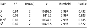
At the beginning, we analysed piglet birth weight itself by a simple LMM. As expected and as widely reported in the literature (e.g. Arango et al., Reference Arango, Misztal, Tsuruta, Culbertson, Holl and Herring2006), a significant sex effect on birth weight existed. Male piglets of line LR (line LW) were about 48 g (46 g) heavier at birth than females. The preliminary analysis of the sample variance of birth weights within one litter and sex per models (1) and (3) resulted in a non-significant sex effect on the variability of birth weight within litter (n = 18366 observations; Table 3). Thus, the following investigations were based on the pooled sample variance in (6) of male and female birth weights within litter in order to account for the difference in mean birth weight.
Testing for the sex effect on the variability of birth weight within litter in the preliminary analysis
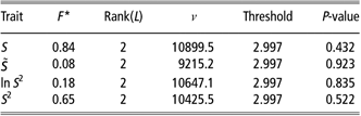
F* denotes the F-test statistic with adjusted denominator degrees of freedom ν; tests were non-significant; S pooled sample standard deviation,  pooled sample standard deviation without weighting the observations, ln S 2 logarithmized pooled sample variance, S 2 pooled sample variance.
Variance components
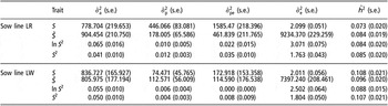
The estimates of variance components and heritabilities are listed in Table 4. The following results are based on an average litter size of  in both sow lines. As an example for Y = ln S 2, the average weight was
 and thereof the average phenotypic variance was estimated as 0.78 (0.62) in sow line LR (sow line LW). The additive genetic variance amounted to 8.33% (8.83%), the paternal variance to 1.28% (0.97%) and the permanent environmental variance accounted for 2.82% (0.00%) of the phenotypic variance in sow line LR (sow line LW). The estimation of heritabilities and their standard errors of the presented models led to similar results within line. The heritability was about 8% in sow line LR and about 10% was estimated in sow line LW.
Comparison of estimated heritabilities  and its standard errors (s.e.)

Estimated variance components:  additive genetic variance,
 variance of boar effect,
 permanent environmental variance,
 residual variance; S pooled sample standard deviation,
 pooled sample standard deviation without weighting the observations, ln S 2 logarithmized pooled sample variance, S 2 pooled sample variance.
If crossbred litters were excluded from the data analysis in sow line LR, then the estimates of heritability were in a range from 10.5% to 12.3%. Thus, heritability turned out to increase about 3% when only purebred litters were involved.
The estimated variance component  turned out to be relatively small especially in sow line LW, see Table 4. The minor contribution of paternal effects on piglet variability coincided with results in the literature (e.g. Damgaard et al., Reference Damgaard, Rydhmer, Løvendahl and Grandinson2003). However, the significance of the boar effect was tested via the restricted likelihood ratio test. The 95% quantile of the 50 : 50 mixture of χ 2-distributions with 0 and 1 degree of freedom is 2.71. As an example for ln S 2 the observed value of the test statistic was 5.84 (3.46) in sow line LR (sow line LW). Thus, in this study the paternal effect was significantly present (line LR: P = 0.008, line LW: P = 0.031). Even if crossbred litters were removed from sow line LR data, the paternal effects were also significant; the observed value of the test statistic was 8.16 (P = 0.002).
Model comparison and residual diagnostics
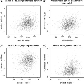
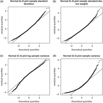
Now the distribution of studentized residuals according to the pooled traits was examined. As an example, Figure 1 related the predictions of the investigated traits with their studentized residuals for sow line LW. For all models the fluctuation margin was relatively small and quite similar. On the basis of the LMM for the traits S,  and ln S 2, it is obvious that the residuals are well evenly distributed. The Q–Q plots in Figure 2 confirm that the distribution of studentized residuals of these responses mainly coincides with a standard normal distribution. Figure 1a displays the estimated within-litter standard deviations and their residuals. But even though a re-weighting estimation technique was used for S, this method was not superior to an unweighted analysis of
 in terms of residual normality, see Figure 1b. Figure 1c displays the estimated log-sample variances and the corresponding studentized residuals. The distribution of the residuals was rather regular but marginally frayed. Figure 1d shows the predicted values of the GLMM (3) on the linearized scale and their residuals. The graphic displays a light trend. This funnel-shaped dispersion is well known from gamma-distributed random variables in an LMM, but in a GLMM the shape should be eliminated by a good choice of the link function. An alternative link function might improve this residual appearance. Having a gamma-distributed error ε the usual link functions like reciprocal and identity were not appropriate to reduce the skewness of the sample variances. A priori, the GLMM was favoured in comparison to the LMM, because the distribution of the trait S 2 is clearly given by the gamma distribution. However, the basic approaches of the LMM are entirely approximate, because the distribution of the responses S and ln S 2 are only asymptotically normal. The residual diagnostics showed that the approximations used for the GLMM estimation methods were not sufficient to reduce the skewness of S 2. The pseudo-response variable Y* in (4) did not follow a normal distribution, as shown by the quantile plot in Figure 2d. The scatterplots of studentized residuals in sow line LR yield similar results.
Analysis of studentized residuals in sow line LW: (a) LMM for the pooled sample standard deviation; (b) LMM for the pooled sample standard deviation without weighting; (c) LMM for the log pooled sample variance; and (d) GLMM for the pooled sample variance.

Q–Q plots of studentized residuals in sow line LW: (a) LMM for the pooled sample standard deviation; (b) LMM for the pooled sample standard deviation without weighting; (c) LMM for the log pooled sample variance; and (d) GLMM for the pooled sample variance.

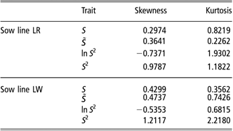
Characteristic moments of the studentized residuals are listed in Table 5. The empirical mean was given by the average of studentized residuals and the empirical variance was calculated by the corresponding sample variance. The empirical skewness and kurtosis were determined per (10) and (11), respectively. The traits S,  and S 2 were positively skewed, whereas ln S 2 was negatively skewed. The estimated characteristic moments of studentized residuals from the LMM for S and ln S 2 coincide most with standard normal moments. The residuals of S are consistently least skew and kurtotic.
Coefficients of skewness and kurtosis for the LMM and the GLMM
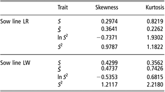
S pooled sample standard deviation,  pooled sample standard deviation without weighting the observations, ln S 2 logarithmized pooled sample variance, S 2 pooled sample variance.
The residual distribution of the trait S is most regular in both lines and the Q–Q plots of the studentized residuals clearly favour that trait. In accordance with graphical results the coefficients of skewness and kurtosis confirm that the LMM (1) for the weighted and pooled sample standard deviation of birth weights within litter is most suitable.
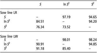
To detect deviations of the presented models in terms of predicted breeding values, the rank correlation of estimates was determined. The differences in rank correlation between the several traits were fairly small. The minimal rank correlation was 94.20% in the comparison of the LMM (1) for the log-sample variance with the GLMM (3) in sow line LR. The maximal rank correlation of 98.24% was determined in sow line LW by comparing the LMM (1) for the sample standard deviation with the GLMM (3). If we picked out those sires within 10% of the lowest breeding values, then the closest agreement of 91.18% was achieved between LMM (1) for S and GLMM (3) in sow line LW. Further results of comparing breeding values are presented in Table 6.
Rank correlations (%) of predicted breeding values (above diagonal) and percentage of matching sires within 10% of the lowest breeding values (below diagonal) for the different traits
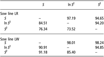
S pooled sample standard deviation, ln S 2 logarithmized pooled sample variance, S 2 pooled sample variance.
Discussion
Heritability and weighting
The estimated heritabilities were in a range from 7.3% to 10.8% (Table 4). These results coincide with the literature, for example Damgaard et al. (Reference Damgaard, Rydhmer, Løvendahl and Grandinson2003) estimated heritability of 8% and Högberg and Rydhmer (Reference Högberg and Rydhmer2000) or Huby et al. (2003) found a heritability of 10% of the within-litter standard deviation without weighting the observations.
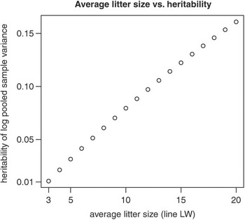
The calculation of heritability in (7) does not lead to a unique value, because the phenotypic variance of the maternal trait depends on the individual weight per litter. The average litter size has a strong influence on heritability. Figure 3 demonstrates the relationship between average litter size and heritability appearing as approximately linear. Litter size is known to vary between populations and within populations, e.g. between progeny of different sires. Thus, the heritability of within-litter variability shows biological variability even when the underlying components of the phenotypic variance are constant in different populations. As a consequence, breeding values for within-litter variability of e.g. sires are more accurate when their daughters exhibit larger litters. Taking the sizes and frequencies of single litters, this biological variation of heritability resulted in a standard deviation of 0.023 in line LR and 0.027 in line LW for the logarithmized and pooled sample variance.
Average litter size v. estimated heritability of the trait S 2 in sow line LW.

Paternal effect on within-litter variance
In this study we assumed an uncorrelated paternal effect on the variability of birth weight in order to account for the effect of boar heterozygosity and assumed  . Since heterozygosity reflects allele combinations, a suitable covariance structure for the boar effect u p may be the dominance relationship matrix. On the other hand, one could think of additive genetic effects of piglet’s sire on within-litter variance. In this case, the numerator relationship matrix would be the appropriate choice for the paternal covariance structure. The latter case would be covered by the model of Sorensen and Waagepetersen (Reference Sorensen and Waagepetersen2003), which would also allow for a genetic covariance between up and the direct genetic effect of progeny. More complicated covariance structures with a combination of additive and dominance effects may match the truth. Our assumption of uncorrelatedness circumvents a decision between additive and/or dominance effects of boar on birth weight variation and may be justified for the purpose of data analysis, especially when the paternal effect is quite small.
Difference between sexes
In the narrow sense the within-litter variance of birth weights is

where Xi (i = 1,…,m) denote piglet birth weights within litter of size m = m 1 + m 2. Therefrom  represent male birth weights and
 female data.
 denotes the average birth weight within litter and
 indicates the average weight per sex g∈{1,2}. Transforming the within-litter variance into terms, which include the sample variance within litter separated by sex (
 and
 ), leads to

Moreover, it is

Thus, the within-litter variance is only partly explained by the pooled within-litter variance  in (6), which includes a correction for the different composition in sex.
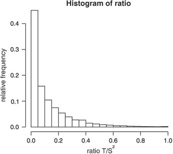
The term T appearing in (13) reflects the difference in mean birth weight per sex. Its contribution on the within-litter variance S 2 cannot be neglected. The average of the ratio T/S 2 was 0.12 with a variability of 0.02, but its median was about 0.06. Surprisingly, the term T explained more than 17% of the total within-litter variance S 2 in 25% of the observations (Figure 4). Hence the minimization of the total within-litter variance by selection is not only achieved by a reduced pooled variability within litter. The difference between average birth weight per sex  and litter mean
 arrests a decrease of the total variability.
Contribution of the difference T in mean birth weight on the total within-litter variance S 2 in terms of the ratio T/S 2.

It might be useful to investigate the coefficient of variation within litter. This issue justifies the association of variability with mean value within litter. Hermesch et al. (2001) analysed the coefficient of within-litter variation and estimated a heritability of 11%, whereas Wolf et al. (Reference Wolf, Žáková and Groeneveld2008) reported a low heritability of 5%.
If we assume a constant value for the sex effect on piglet birth weight in all litters, then we immediately subtract the sex effect from male birth weights to eliminate the sex contribution on the total within-litter variance; the degrees of freedom are (m−1). To prove this possibility, we have separately analysed piglet birth weight for all classes of parity. The sex effect ranged from 42.58 to 59.65 g in line LR and from 34.81 to 57.04 g in line LW. Because the effect of sex varied over parities, there is further need to analyse whether genetics influences the difference in male and female birth weights.
In other studies (Högberg and Rydhmer, Reference Högberg and Rydhmer2000; Damgaard et al., Reference Damgaard, Rydhmer, Løvendahl and Grandinson2003; Huby et al., 2003), the sex effect on birth weight has not been explicitly considered. We repeated that basic approach and took the total within-litter variance in (12) or its transformations as the trait of sow. We studied heritability and found small differences from our previous results in Table 4. In sow line LR the estimates of heritability decreased about 1%; the heritability of S 2 was 7.23%, for ln S 2 it was 6.77% and for S we obtained 6.24%. Whereas in sow line LW the estimates of heritability were slightly increased about 1%, for S 2 heritability was estimated as 11.69%, for ln S 2 we achieved 9.30% and for S it was 11.80%. Thus, it seems less important to account for the different contributions of mean birth weight per sex on the variability within litter when only the estimation of heritability is of interest. Nevertheless, only the pooled sample variance takes into account the sex effect on mean birth weight and is therefore an unbiased estimator for birth weight variability within litter.
Conclusions
In summary, a significant sex effect on piglet birth weight but not on its variability was found and this situation can be appropriately handled by the pooled within-litter variance of male and female birth weights. Adequate weighting of the trait is required to account for different litter sizes and along with that to estimate the parameters more precisely. The LMM for S and ln S 2 are suitable to analyse the genetic effect on the within-litter variance. Due to the remaining skewness of the studentized residuals of the GLMM for S 2 we cannot recommend this alternative approach. The residual diagnostics favour model (1) for the pooled sample standard deviation to fit the within-litter variance. Beside fixed effects, this model attended to the additive genetic effect of sow, the effect of boar heterozygosity and permanent environmental effects.
Acknowledgement
We thank Hubert Henne from the Bundeshybridzuchtprogramm (Züchtungszentrale Deutsches Hybridschwein GmbH) for providing the extensive data.
The research project was financially supported by the H. Wilhelm Schaumann Stiftung.