1. Introduction
Mixing in stratified fluids is a topic of fundamental importance in nature. Of particular interest is the case in which mixing results in trapping phenomena, such as those of pollutants in oil spills and other effluents in similar environments. Here, we focus on the case of buoyant turbulent miscible jets/plumes in stable ambient fluid stratification and the mixing and trapping observable in such set-ups.
There is a wealth of literature on buoyant turbulent jets, particularly following the seminal work of Morton, Taylor & Turner (Reference Morton, Taylor and Turner1956) – for extensive reviews on the subject, see for example the classic text by Fischer et al. (Reference Fischer, List, Koh, Imberger and Brooks1979), and more recent review articles by Hunt & van den Bremer (Reference Hunt and van den Bremer2010) and Woods (Reference Woods2010).
Despite the extensive literature on this subject, many open questions remain, particularly regarding the mathematical foundation of predictions based on Morton–Taylor–Turner (MTT) models. In particular, the rigorous characterization of trapping versus escaping of buoyant jets and plumes and its dependence on the functional form of stratification profiles has not been fully explored. Such a study would naturally lead to a search for which ambient fluid density profile constitutes an optimal mixer for trapping. In turn, this would lead to establishing the asymptotic properties of jet/plume densities for sufficiently weak mixers for escaping at large distances from their source. Such questions are relevant in a variety of physical settings, among which the most common is probably that of atmospheric inversions with smoke stack discharges. Notably, the work by Briggs et al. (Briggs Reference Briggs1965; Hanna, Briggs & Hosker Reference Hanna, Briggs and Hosker1983) presented trapping criteria for smoke stack pollution under sharply stratified atmospheric conditions.
Here, we carry out a mathematically rigorous analysis of the MTT model for a broad class of ambient density profiles, and experimentally verify their predictions. Our building block (both analytically and experimentally) is a two-layer density configuration. We explore the problem of characterizing and measuring a critical phenomenon that can arise in such ambient fluid set-ups. By varying the distance of a jet nozzle suspended below a density transition, an analytical and experimental critical length is determined: jets at greater distances than this length will be completely trapped, while jets with nozzles nearer the transition will escape. Somewhat related experimental studies have appeared in the literature involving slit injections (Wallace & Sheff Reference Wallace and Sheff1987; Noh, Fernando & Ching Reference Noh, Fernando and Ching1992; Ching, Fernando & Noh Reference Ching, Fernando and Noh1993). These references explored plume penetration behaviour through a sharp density transition as various parameters were varied. The basic observation in these line-source studies was that strong penetration occurs when either the momentum is large or the stratification is weak. However, these experiments were conducted in a fixed thickness of top and bottom layer, and did not focus on determining a critical length, and a companion mathematical analysis was not developed.
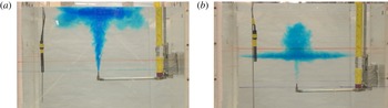
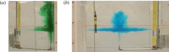
A schematic of our experimental set-up is presented as an actual picture from our experiment in figure 1. This depicts typical trapping/escape outcomes in our experiments. The analytical counterpart of our study provides a mathematically rigorous proof that step-like stratifications of the ambient fluid are, under appropriate circumstances, the optimal mixers of the miscible jet fluid with the environment. As a corollary, we are able to provide a proof of the trapping/escaping criteria presented by Caulfield & Woods (Reference Caulfield and Woods1998) through Gronwall-like estimates on solutions of the MTT hierarchy, including the solution existence/breakdown intervals. An exact formula for step-function stratifications employing nonlinear jump conditions follows from this analysis. This formula compares favourably at a quantitative level with the data from an extensive experimental campaign to isolate the functional dependence of the critical distance with respect to the physical parameters. We remark that prior formulae, derived in Adalsteinsson et al. (Reference Adalsteinsson, Camassa, Harenberg, Lin, McLaughlin, Mertens, Reis, Schlieper and White2011), presented a critical height formula in homogeneous background fluids; however, this result does not account for the important mixing that occurs when passing through the sharp background-density layer. The new formulae derived here take into account this critical additional strong mixing, resulting in an accurate prediction of the experimental critical lengths we observe. Our optimal mixing result is obtained through the direct comparison between the general system and the new exact solution (which now accounts for mixing in the density transition layer) by using Gronwall-like estimates. While at first sight it may seem intuitively obvious that the step density profile would provide the optimal mixer, given that such ambient fluid density profile maximizes the local buoyancy of the jet on its way to the density transition, a closer inspection shows that this is not the case. Our analysis proves that the initial mixing by the Gaussian closure model with a homogeneous background fluid is the weakest mixer amongst all stable stratifications. However, the extra mixing at the density step under this (Gaussian) closure restores the optimality of the two-layer stratification. The competition of weaker mixing in the bulk with enhanced mixing at the transition layer seems rather subtle and requires careful mathematical analysis. Alternatively, for the top-hat closure, the higher contrast of jet density within a homogeneous lower fluid environment indeed results in the strongest initial mixing, while the two-layer stratification remains the strongest mixer even under this closure when mixing is measured across the full density transition layer.
Water jet escaping (a) and trapping (b) in a sharp ambient density transition. The experiments consist of firing a miscible jet of initial density
 ${\it\rho}_{j}(0)=0.998~\text{g}~\text{cm}^{-3}$
with fixed volumetric flow rate of
 $15~\text{ml}~\text{s}^{-1}$
, within an ambient fluid with bottom density
 ${\it\rho}_{b}=1.055~\text{g}~\text{cm}^{-3}$
and top density
 ${\it\rho}_{t}=1.043~\text{g}~\text{cm}^{-3}$
. The Reynolds number based on the nozzle diameter is approximately
 $Re\simeq 4600$
. The distance between nozzle and transition layer is (a) 4 cm and (b) 12 cm. The nozzle diameter is 0.4572 cm and the tank width is 72.4 cm.

The layout of this paper is as follows. We first study the general MTT model to establish mathematical criteria for solution existence and their finite-distance breakdown in § 2.1. In § 2.2, we derive sharper bounds for general ambient density profiles using Gronwall-like estimates, and study asymptotic behaviours in homogeneous background. We then apply these results to a family of stratification profiles of relevance for theoretical and experimental investigations in § 2.3. The estimates here and in § 2.2 provide the rigorous framework for numerical observations in Caulfield & Woods (Reference Caulfield and Woods1998) reporting trapping/escaping criteria for a family of power-law density–height dependence. An exact formula for the case of step density–height dependence is presented next, § 2.4, under physically motivated jump conditions, which for their rigorous justification requires a study, carried out in § 2.5, of linear stratifications (or, more generally, by approximating the step function by a general family of smooth functions). The optimal mixer results for a broad class of stable stratifications, including their non-intuitive behaviour dependence upon turbulent closure schemes, are presented in § 2.6. In § 3, we describe the experimental methods we use. In § 4, we compare the experimental results with the predictive capabilities of the theory, both by establishing the critical height and by demonstrating the optimality of two-layer set-ups as mixers. We additionally explore the combined fine-tuning effects of using variable (local Richardson-number-dependent) entrainment along with modelling with a smooth, sharp density transition. Finally, a direct application to the Deepwater Horizon oil spill in the Gulf of Mexico of the optimal mixing result is presented to close this section. A discussion session, § 5, concludes the paper. Technical details are reported in the four appendices.
2. Theoretical results
2.1. Model and solution existence criterion
We begin by considering the reduced model in Morton et al. (Reference Morton, Taylor and Turner1956),
 $$\begin{eqnarray}(b^{2}w)^{\prime }=2{\it\alpha}bw,\quad (b^{2}w^{2})^{\prime }=2g{\it\lambda}^{2}b^{2}{\it\theta},\quad (b^{2}w{\it\theta})^{\prime }={\it\rho}_{a}^{\prime }(b^{2}w)/({\it\Lambda}{\it\rho}_{b}),\end{eqnarray}$$
where primes denote differentiation
 $\text{d}/\text{d}z$
,
 $b(z)$
is the jet width,
 $w(z)$
is the vertical jet velocity,
 ${\it\theta}(z)=({\it\rho}_{a}(z)-{\it\rho}_{j}(z))/{\it\rho}_{b}$
is the density anomaly, and
 ${\it\rho}_{a}(z)$
is the ambient background density. Here the constants are the gravitational acceleration
 $g$
, oriented downwards with respect to the vertical coordinate
 $z$
, the entrainment coefficient
 ${\it\alpha}$
, the mixing coefficient
 ${\it\lambda}$
(Morton et al.
Reference Morton, Taylor and Turner1956; Fischer et al.
Reference Fischer, List, Koh, Imberger and Brooks1979), and
 ${\it\Lambda}={\it\lambda}^{2}/(1+{\it\lambda}^{2})$
, respectively. Letting
 $q=b^{2}w$
,
 $m=b^{4}w^{4}$
and
 ${\it\beta}=b^{2}w{\it\theta}$
, system (2.1) becomes
 $$\begin{eqnarray}q^{\prime }=2{\it\alpha}m^{1/4},\quad m^{\prime }=4g{\it\lambda}^{2}q{\it\beta},\quad {\it\beta}^{\prime }={\it\rho}_{a}^{\prime }q/({\it\Lambda}{\it\rho}_{b}),\end{eqnarray}$$
describing the volume, momentum and buoyancy fluxes, respectively. We note that this model in (2.1) employs a constant entrainment coefficient; below, in § 4, we discuss in detail different choices of this constant, as well as examining a nonlinear local Richardson-number-dependent entrainment law originally presented by Priestley & Ball (Reference Priestley and Ball1955). The initial conditions for this system are discussed below in (2.36). The model in this form also employs the Gaussian plume closure, which assumes that the velocity and density profiles are self-similar Gaussian functions of cylindrical radial coordinate with ratio of half-width scaling coefficients between velocity and density defined as the constant
 ${\it\lambda}$
. A variant of system (2.1) would replace
 ${\it\Lambda}$
with unity and
 ${\it\lambda}=1/\sqrt{2}$
for the so-called ‘top-hat’ closure model. (This alternative closure is explored analytically below, with appropriately modified initial conditions.)
For a stably stratified environment (
 ${\it\rho}_{a}^{\prime }\leqslant 0$
), the solution to (2.2) exists in
 $[0,z_{s})$
, where
 $z_{s}$
is the location where momentum vanishes (
 $m(z_{s})=0$
), provided the initial values of
 $q(0)=Q_{0}$
,
 $m(0)=M_{0}$
and
 ${\it\beta}(0)=B_{0}$
are all positive. The proof of existence is divided into two regions, namely
 $[0,z_{ne}]$
and
 $[z_{ne},z_{s})$
, where
 $z_{ne}$
is the neutral buoyant location (
 ${\it\beta}(z_{ne})=0$
).
The existence of solutions can be established by the bounds
 $$\begin{eqnarray}\left.\begin{array}{@{}c@{}}\displaystyle Q_{0}\leqslant q\leqslant 2Q_{0}\text{e}^{Kz},\quad M_{0}\leqslant m\leqslant M_{0}\sinh (Kz),\quad 0\leqslant {\it\beta}\leqslant B_{0}\quad \text{in }[0,z_{ne}],\\ \displaystyle Q_{0}\leqslant q\leqslant 2Q_{0}\text{e}^{Kz},\quad 0<m\leqslant m(z_{ne}),\quad -\infty <{\it\beta}\leqslant 0\quad \text{in }[z_{ne},z_{s}),\end{array}\right\}\end{eqnarray}$$
through the following estimate. Initially,
 $Q_{0}$
,
 $M_{0}$
and
 $B_{0}$
are all positive, and, as long as
 $m$
stays positive, the volume equation in system (2.2) shows that
 $q$
is increasing, and hence must be positive. As
 $q\geqslant 0$
,
 ${\it\beta}$
is decreasing but still positive in
 $[0,z_{ne}]$
, so that
 $m$
is increasing,
 $m\geqslant M_{0}>0$
, by the momentum equation in (2.2). For
 $z\geqslant z_{ne}$
, note that
 $z_{ne}$
also plays the role of locating where the maximum momentum occurs, since
 $m$
is decreasing after
 $z_{ne}$
; for as long as
 $m$
does not decrease to zero,
 $q$
keeps increasing, and
 ${\it\beta}$
keeps decreasing.
Upper bounds for
 $q$
and
 $m$
are sufficient to show existence in
 $[0,z_{ne}]$
, as
 $0\leqslant {\it\beta}\leqslant B_{0}$
. Non-dimensionalizing the
 $q$
and
 $m$
equations in (2.2) by
 $\bar{q}=q/Q_{0}$
and
 $\bar{m}=m/M_{0}$
, the differential inequalities
 $$\begin{eqnarray}\displaystyle & \displaystyle \bar{q}^{\prime }=\frac{2{\it\alpha}M_{0}^{1/4}}{Q_{0}}\bar{m}^{1/4}\leqslant \frac{2{\it\alpha}M_{0}^{1/4}}{Q_{0}}\bar{m}, & \displaystyle\end{eqnarray}$$
 $$\begin{eqnarray}\displaystyle & \displaystyle \bar{m}^{\prime }=\frac{4g{\it\lambda}^{2}{\it\beta}Q_{0}}{M_{0}}\bar{q}\leqslant \frac{4g{\it\lambda}^{2}B_{0}Q_{0}}{M_{0}}\bar{q} & \displaystyle\end{eqnarray}$$
 $\bar{m}>1$
in
 $[0,z_{ne}]$
. Let
 $K$
be the larger of
 $2{\it\alpha}M_{0}^{1/4}/Q_{0}$
and
 $4g{\it\lambda}^{2}Q_{0}B_{0}/M_{0}$
. Comparing the system in (2.4) with the auxiliary linear system
 $\bar{q}_{b}^{\prime }=K\bar{m}_{b}$
and
 $\bar{m}_{b}^{\prime }=K\bar{q}_{b}$
yields
 $$\begin{eqnarray}1\leqslant \bar{q}\leqslant {\textstyle \frac{1}{2}}[\text{e}^{Kz}+\text{e}^{-Kz}]=\bar{q}_{b}(z),\quad 1\leqslant \bar{m}\leqslant {\textstyle \frac{1}{2}}[\text{e}^{Kz}-\text{e}^{-Kz}]=\bar{m}_{b}(z),\end{eqnarray}$$
so that
 $\bar{q}$
and
 $\bar{m}$
have upper and lower bounds in any finite interval
 $[0,z_{ne}]$
.
Next, for
 $z>z_{ne}$
,
 $\bar{m}$
decreases, and the bounds for
 $\bar{q}$
in (2.5) hold until
 $\bar{m}(z_{R})=1$
for some
 $z_{R}\in (z_{ne},z_{s})$
. Further, we point out that the bounds in (2.5) actually apply for all
 $z\in [0,z_{R}]$
.
Continuing beyond
 $z_{R}$
from (2.4a
), the differential inequality
 $$\begin{eqnarray}\displaystyle \bar{q}^{\prime }\leqslant 2{\it\alpha}M_{0}^{1/4}/Q_{0}\leqslant K & & \displaystyle\end{eqnarray}$$
holds for
 $z\geqslant z_{R}$
, hence
 $\bar{q}\leqslant \bar{q}(z_{R})+K(z-z_{R})$
. Stitching this bound together with (2.5b
) gives
 $$\begin{eqnarray}\displaystyle \bar{q}(z_{R})\leqslant {\textstyle \frac{1}{2}}[\text{e}^{Kz_{R}}+\text{e}^{-Kz_{R}}]\leqslant \text{e}^{Kz_{R}}\leqslant \text{e}^{Kz}, & & \displaystyle\end{eqnarray}$$
and noting the functional relation
 $K(z-z_{R})<\text{e}^{K(z-z_{R})}\leqslant \text{e}^{Kz}$
yields an upper bound
 $$\begin{eqnarray}\displaystyle \bar{q}\leqslant 2\text{e}^{Kz} & & \displaystyle\end{eqnarray}$$
for
 $z\geqslant z_{R}$
, so that an overall bound for dimensional
 $q$
is
 $$\begin{eqnarray}\displaystyle q\leqslant 2Q_{0}\text{e}^{Kz},\quad \text{for }z\in [0,z_{s}). & & \displaystyle\end{eqnarray}$$
In summary, for
 $z>z_{ne}$
,
 $m$
decreases, and, as long as
 $m$
stays positive,
 $0<m<m(z_{ne})$
,
 $Q_{0}\leqslant q\leqslant 2Q_{0}\exp (Kz)$
, and
 $|{\it\beta}|$
also does not blow up in finite heights
 $z$
; since
 $q$
has a smooth integrable lower bound, this allows one to bracket
 ${\it\beta}$
by
 $$\begin{eqnarray}\displaystyle \left.\begin{array}{@{}c@{}}\displaystyle B_{0}\geqslant {\it\beta},\\ \displaystyle {\it\beta}=B_{0}-\int _{0}^{z}\frac{|{\it\rho}_{a}^{\prime }|}{{\it\Lambda}{\it\rho}_{b}}q\,\text{d}s\geqslant B_{0}-\int _{0}^{z}\frac{2|{\it\rho}_{a}^{\prime }|Q_{0}}{{\it\Lambda}{\it\rho}_{b}}\text{e}^{Ks}\,\text{d}s,\end{array}\right\} & & \displaystyle\end{eqnarray}$$
so that
 $|{\it\beta}|$
stays bounded for the entire interval
 $z\in [0,z_{s})$
, guaranteeing solution existence therein.
The above estimates show that the breakdown criterion for system (2.2) can only be
 $m=0$
, which can only happen if
 $z=z_{s}$
, whose location (finite or infinite) depends on the initial data, parameters and density profile. First, observe that the system (2.2) is non-Lipschitz at
 $m=0$
. Second, if
 $m$
were to vanish, then, by the relation
 $b=q/m^{1/4}$
, and the boundedness of
 $q$
, just established,
 $b$
would blow up at distance
 $z_{s}$
.
We next want to discuss the finiteness or otherwise of the singularity location
 $z_{s}$
. First, we note that, if
 $z_{ne}=\infty$
, i.e.
 ${\it\beta}$
never touches zero, the solution is global since by definition
 $z_{ne}\leqslant z_{s}$
. In fact, in this case,
 $q$
and
 $m$
are increasing and bounded by the first two estimates in (2.3), while
 ${\it\beta}$
remains positive for all
 $z$
.
Second, suppose
 $z_{ne}$
were to be a finite number. In this case, there exists
 $z_{{\it\gamma}}>z_{ne}$
such that
 ${\it\beta}(z_{{\it\gamma}})<{\it\gamma}<0$
for some negative number
 ${\it\gamma}$
, provided
 ${\it\rho}_{a}^{\prime }(z_{ne})<0$
. (Note that, if
 ${\it\rho}_{a}(z)$
is constant for all
 $z\geqslant z_{ne}$
, i.e.
 ${\it\beta}\equiv 0$
after
 $z_{ne}$
, then momentum would be conserved for all
 $z\geqslant z_{ne}$
, so that
 $z_{s}$
would stay at
 $\infty$
; more complicated cases in which
 ${\it\rho}_{a}$
is continuous but not differentiable can be handled similarly.) Now, assuming the existence of
 ${\it\gamma}<0$
and integrating the differential inequality
 $$\begin{eqnarray}\displaystyle m^{\prime }=4g{\it\lambda}^{2}q{\it\beta}<4g{\it\lambda}^{2}Q_{0}{\it\gamma} & & \displaystyle\end{eqnarray}$$
from
 $z_{{\it\gamma}}$
to any
 $z>z_{{\it\gamma}}$
yields
 $$\begin{eqnarray}\displaystyle m\leqslant M(z_{{\it\gamma}})+4g{\it\lambda}^{2}Q_{0}{\it\gamma}(z-z_{{\it\gamma}}), & & \displaystyle\end{eqnarray}$$
which implies that
 $m$
must vanish within a finite distance
 $z\equiv z_{s}$
, since the last term in this inequality is a linearly decaying function of increasing
 $z$
. Hence, under the above assumptions,
 $z_{s}$
is finite.
2.2. More delicate bounds and asymptotic relations
Sharper bounds for
 $q$
and
 ${\it\beta}$
in system (2.2) can be derived by using Gronwall-like estimates. Combining (2.2b
) and (2.2a
) yields
 $$\begin{eqnarray}2{\it\alpha}m^{1/4}\frac{\text{d}m}{\text{d}q}=\frac{8{\it\alpha}}{5}\frac{\text{d}}{\text{d}q}(m^{5/4})=4g{\it\lambda}^{2}{\it\beta}q,\end{eqnarray}$$
and since
 ${\it\beta}\leqslant B_{0}$
, the inequality
 $$\begin{eqnarray}\displaystyle \frac{8{\it\alpha}}{5}\frac{\text{d}}{\text{d}q}(m^{5/4})\leqslant 4g{\it\lambda}^{2}B_{0}q & & \displaystyle\end{eqnarray}$$
gives, by the Gronwall lemma, a bound on
 $m(q)$
:
 $$\begin{eqnarray}m(q)\leqslant \left(\frac{5g{\it\lambda}^{2}B_{0}}{4{\it\alpha}}(q^{2}-Q_{0}^{2})+m(Q_{0})^{5/4}\right)^{4/5}.\end{eqnarray}$$
Solving for
 $q$
in (2.2) taking into account this inequality yields the estimate
 $$\begin{eqnarray}Z(q)\equiv \frac{1}{2{\it\alpha}}\int _{Q_{0}}^{q}\left(\frac{5g{\it\lambda}^{2}B_{0}}{4{\it\alpha}}(s^{2}-Q_{0}^{2})+m(Q_{0})^{5/4}\right)^{-1/5}\text{d}s\leqslant z(q).\end{eqnarray}$$
The left-hand side of (2.16) defines the inverse function of
 $Q_{h}(Z)$
for the solution to the homogeneous case, written with new variables
 $Q_{h}$
and
 $M_{h}$
,
 $$\begin{eqnarray}Q_{h}^{\prime }=2{\it\alpha}M_{h}^{1/4},\quad M_{h}^{\prime }=4g{\it\lambda}^{2}B_{0}Q_{h},\quad B=B_{0}.\end{eqnarray}$$
Hence, for the same value of volume flux
 $Q_{h}=q$
, the corresponding height
 $Z(Q_{h})$
in homogeneous ambient fluid is less than or equal to the height
 $z(q)$
for the general case. Given that
 $Q_{h}(z)$
is a strictly increasing function of height
 $z$
, the value of the volume flux
 $\tilde{Q}_{h}$
defined by the equality
 $Z(\tilde{Q}_{h})=z(q)$
must satisfy
 $\tilde{Q}_{h}(Z)\geqslant Q_{h}(Z)=q(z)$
, i.e. for any fixed distance
 $z$
,
 $q(z)\leqslant Q_{h}(z)$
.
Next, integrating the
 $M_{h}$
and
 $m$
equations and using the same inequality
 ${\it\beta}\leqslant B_{0}$
yields the relation
 $$\begin{eqnarray}\displaystyle m=M_{0}+\int _{0}^{z}4g{\it\lambda}^{2}{\it\beta}q\,\text{d}s\leqslant M_{0}+\int _{0}^{z}4g{\it\lambda}^{2}B_{0}Q_{h}\,\text{d}s=M_{h}. & & \displaystyle\end{eqnarray}$$
Thus, we have the following bounds on the general system in terms of the homogeneous ambient fluid variables,
 $$\begin{eqnarray}\displaystyle q(z)\leqslant Q_{h}(z),\quad m(z)\leqslant M_{h}(z), & & \displaystyle\end{eqnarray}$$
provided the solution of (2.2) exists.
An asymptotic relation for
 $z\rightarrow \infty$
can be found by using the inverse integral solutions of (2.17), viewed as functions of
 $Q_{h}$
and
 $M_{h}$
, respectively:
 $$\begin{eqnarray}\displaystyle & \displaystyle z(Q_{h})=\frac{(Q_{h}-Q_{0})^{4/5}}{2{\it\alpha}}\int _{0}^{1}\left(M_{0}^{5/4}+\frac{5g{\it\lambda}^{2}B_{0}}{4{\it\alpha}}r(2Q_{0}+(Q_{h}-Q_{0})r)\right)^{-1/5}\text{d}r, & \displaystyle\end{eqnarray}$$
 $$\begin{eqnarray}\displaystyle & \displaystyle z(M_{h})=\frac{M_{h}-M_{0}}{4g{\it\lambda}^{2}B_{0}}\int _{0}^{1}\left(Q_{0}^{2}+\frac{4{\it\alpha}}{5g{\it\lambda}^{2}B_{0}}((M_{0}+(M_{h}-M_{0})r)^{5/4}-M_{0}^{5/4})\right)^{-1/2}\text{d}r.\qquad & \displaystyle\end{eqnarray}$$
 $Q_{h}\sim C_{1}B_{0}^{1/3}z^{5/3}$
and
 $M_{h}\sim C_{2}B_{0}^{4/3}z^{8/3}$
as
 $z\rightarrow \infty$
, where the constants are
 $C_{1}=(1944g{\it\lambda}^{2}{\it\alpha}^{4}/625)^{1/3}$
and
 $C_{2}=(9{\it\alpha}g{\it\lambda}^{2}/5)^{4/3}$
. Note that, following the previous argument, if a priori it is known that
 ${\it\beta}>{\it\beta}_{\infty }>0$
, a lower bound for
 $q$
can be obtained by
 $$\begin{eqnarray}\frac{1}{2{\it\alpha}}\int _{Q_{0}}^{q}\left(\frac{5g{\it\lambda}^{2}{\it\beta}_{\infty }}{4{\it\alpha}}(s^{2}-Q_{0}^{2})+m(Q_{0})^{5/4}\right)^{-1/5}\text{d}s\geqslant z(q),\end{eqnarray}$$
and since
 $m(Q_{0})$
and
 $Q_{0}$
are positive, by changing variables
 $s=Q_{0}+(q-Q_{0})r$
, it follows that
 $$\begin{eqnarray}z(q)<\frac{(q-Q_{0})^{4/5}}{(40g{\it\lambda}^{2}{\it\alpha}^{4}{\it\beta}_{\infty })^{1/5}}\int _{0}^{1}(r(2Q_{0}+(q-Q_{0})r))^{-1/5}\,\text{d}r<\left(\frac{q-Q_{0}}{C_{1}{\it\beta}_{\infty }^{1/3}}\right)^{3/5}.\end{eqnarray}$$
Thus, a lower bound for
 $q$
follows by (2.23)
 $$\begin{eqnarray}q(z)>C_{1}{\it\beta}_{\infty }^{1/3}z^{5/3}.\end{eqnarray}$$
2.3. Analytical trapping/escaping criterion for more general profiles
In system (2.2), for algebraic density decay rates,
 ${\it\rho}_{a}^{\prime }=Cz^{p}$
(
 $C<0$
), a critical power
 $p=-8/3$
separates two distinct behaviours: if
 $p>-8/3$
, the jet/plume must trap; while for
 $p<-8/3$
either trapping or escaping could happen (Caulfield & Woods Reference Caulfield and Woods1998). We prove this below, and also show that the result extends to asymptotic relations
 ${\it\rho}_{a}^{\prime }\sim Cz^{p}$
as
 $z\rightarrow \infty$
, depending on the constant
 $|C|$
. (Note that this constant is set by the overall density difference if the power-law dependence on
 $z$
is strictly imposed throughout the domain; our result is slightly more general in that this dependence is only used asymptotically for large
 $z$
.) We remark that this critical behaviour, which was originally observed numerically by Caulfield & Woods (Reference Caulfield and Woods1998), has been recently investigated by Kaye & Scase (Reference Kaye and Scase2011) using formal asymptotic tools which have provided a partial insight into this phenomenon. This study, under the restrictive assumption that the plume is straight-sided (purely conical) and by assuming infinite existence domain for the solution, successfully yields the critical exponent
 $p=-8/3$
obtained by Caulfield & Woods (Reference Caulfield and Woods1998). Our results below use integral estimates to achieve mathematical rigour and avoid formal assumptions; the techniques we use further extend and prove the existence of this critical behaviour for a much broader class of background density profiles.
To construct a rigorous mathematical proof, we use the solution existence criterion established in § 2.1: since
 ${\it\rho}_{a}^{\prime }\sim Cz^{p}$
as
 $z\rightarrow \infty$
, for
 $z$
large enough,
 ${\it\beta}^{\prime }$
must be strictly negative so that, if
 $z_{ne}$
is finite,
 ${\it\beta}$
must be less than some value
 ${\it\gamma}<0$
. Hence, by § 2.1, existence of finite
 $z_{ne}$
implies breakdown of the system, which means trapping must occur. Conversely, if
 ${\it\beta}>0$
, the solution of (2.2) is global and the injection rises indefinitely.
Next, to prove trapping, suppose
 ${\it\beta}>0$
for all
 $z$
; since
 ${\it\beta}$
is monotonically decreasing, so
 ${\it\beta}\rightarrow {\it\beta}_{\infty }\geqslant 0$
as
 $z\rightarrow \infty$
, and
 ${\it\rho}_{a}^{\prime }\sim Cz^{p}$
for
 $p\geqslant -8/3$
as
 $z\rightarrow \infty$
implies
 ${\it\rho}_{a}^{\prime }z^{5/3}\notin \mathscr{L}^{1}(\mathbb{R}^{+})$
. With
 ${\it\beta}_{\infty }\geqslant 0$
, either
 ${\it\beta}_{\infty }>0$
,
 $$\begin{eqnarray}{\it\beta}\leqslant B_{0}-\frac{C_{1}}{{\it\Lambda}{\it\rho}_{b}}\int _{0}^{z}|{\it\rho}_{a}^{\prime }|{\it\beta}_{\infty }^{1/3}z^{5/3}\,\text{d}s<0,\end{eqnarray}$$
for
 $z$
large enough, or
 ${\it\beta}_{\infty }=0$
, for which the above lower estimate for
 $q$
fails. For the purpose of determining whether
 ${\it\rho}_{a}^{\prime }q$
belongs to
 $\mathscr{L}^{1}(\mathbb{R}^{+})$
, it is sufficient to estimate
 $q$
for finite
 $z$
: when
 ${\it\beta}_{\infty }=0$
, for any fixed
 $z_{c}<\infty$
,
 ${\it\beta}(z_{c})={\it\beta}_{c}>0$
. Confining
 $z\in [0,z_{c})$
, and following the same steps as above, we have
 $q(z)>C_{1}{\it\beta}_{c}^{1/3}z^{5/3}=C_{1}{\it\beta}(z)^{1/3}z^{5/3}$
. The
 ${\it\beta}$
equation in (2.2) thus yields
 $$\begin{eqnarray}({\it\beta}(z))^{2/3}\leqslant B_{0}^{2/3}-\frac{2}{3}\left(\frac{C_{1}}{{\it\Lambda}{\it\rho}_{b}}\int _{0}^{z}|{\it\rho}_{a}^{\prime }|s^{5/3}\,\text{d}s\right)<0\end{eqnarray}$$
for
 $z$
large enough. Hence
 $z_{ne}$
must be finite, and trapping must occur.
On the other hand, if
 ${\it\rho}_{a}^{\prime }z^{5/3}\in \mathscr{L}^{1}(\mathbb{R}^{+})$
, since
 $q\leqslant Q_{h}$
(cf. § 2.2), with
 $Q_{h}$
the solution to the system of equations with homogeneous ambient density (2.17), we have the following estimate on
 ${\it\beta}$
:
 $$\begin{eqnarray}{\it\beta}(z)=B_{0}+\int _{0}^{z}\frac{{\it\rho}_{a}^{\prime }}{{\it\Lambda}{\it\rho}_{b}}q\,\text{d}s\geqslant B_{0}-\int _{0}^{z}\frac{|{\it\rho}_{a}^{\prime }|}{{\it\Lambda}{\it\rho}_{b}}Q_{h}\,\text{d}s.\end{eqnarray}$$
Since we know
 $Q_{h}\sim C_{1}B_{0}^{1/3}z^{5/3}$
as
 $z\rightarrow \infty$
(see § 2.2), a sufficiently small
 $|C|$
prevents
 ${\it\beta}=0$
at finite distances and leads to escaping, while a large value of
 $|C|$
, through estimate (2.26), again forces trapping as
 ${\it\beta}(z)$
vanishes for some finite value
 $z$
.
2.4. Exact formula with two-layer ambient profile
We now focus on a generalized MTT system for the behaviour of a turbulent jet/plume in a sharply stratified ambient fluid (represented by a step function,
 ${\it\rho}={\it\rho}_{b}$
for
 $z<L$
and
 ${\it\rho}={\it\rho}_{t}$
when
 $z>L$
),
 $$\begin{eqnarray}(b^{2}w)^{\prime }=2{\it\alpha}bw,\quad (b^{2}w^{2})^{\prime }=2g{\it\lambda}^{2}b^{2}{\it\theta},\quad (b^{2}w{\it\theta})^{\prime }=-({\it\theta}_{f}{\it\delta}(z-L)/{\it\Lambda})b^{2}w,\end{eqnarray}$$
where
 ${\it\theta}_{f}=({\it\rho}_{b}-{\it\rho}_{t})/{\it\rho}_{b}$
,
 $L$
is the distance between the nozzle and the transition layer, and
 ${\it\delta}$
is the Dirac delta function. Note that this is a nonlinear differential equation with a discontinuous coefficient, so that a selection criterion for a physical solution is needed.
A mathematical formula for a critical length can be shown to be accurate when compared to experimental data with explicit quadrature involving a hyper-geometric special function (see e.g. figure 5 below)
 $$\begin{eqnarray}L^{\ast }=L_{0}\int _{1}^{A^{\ast }}\!\frac{\text{d}s}{\sqrt{s^{5/4}+{\it\epsilon}-1}},\end{eqnarray}$$
where the parameter
 $$\begin{eqnarray}\displaystyle {\it\epsilon}=\frac{5(1+{\it\lambda}^{2}){\rm\Delta}\bar{{\it\rho}}r_{0}g}{16\sqrt{2}{\it\alpha}w_{0}^{2}} & & \displaystyle\end{eqnarray}$$
is proportional to the square of the Richardson number introduced in Fischer et al. (Reference Fischer, List, Koh, Imberger and Brooks1979), the upper limit of integration is
 $$\begin{eqnarray}\displaystyle A^{\ast }=(1+{\it\epsilon}(({\rm\Delta}\bar{{\it\rho}}/{\it\theta}_{f})^{2}-1))^{4/5} & & \displaystyle\end{eqnarray}$$
and the length scale
 $L_{0}$
is given by the combination of initial conditions and entrainment parameters as
 $$\begin{eqnarray}\displaystyle L_{0}=\left(\frac{5r_{0}w_{0}^{2}}{16\sqrt{2}g(1+{\it\lambda}^{2}){\it\alpha}{\rm\Delta}\bar{{\it\rho}}}\right)^{1/2}. & & \displaystyle\end{eqnarray}$$
Here
 ${\it\rho}_{j}(0)$
,
 $r_{0}$
and
 $w_{0}$
are the physical initial jet density, radius and velocity, respectively, and
 ${\rm\Delta}\bar{{\it\rho}}=({\it\rho}_{b}-{\it\rho}_{j}(0))/{\it\rho}_{b}$
. (We remark that a different formula for
 $L^{\ast }$
,
 $L_{m}^{\ast }$
say, was presented in Adalsteinsson et al. (Reference Adalsteinsson, Camassa, Harenberg, Lin, McLaughlin, Mertens, Reis, Schlieper and White2011); the upper limit of integration in (2.29) was taken to be
 $A_{m}^{\ast }\equiv (1+{\it\epsilon}(({\it\theta}_{0}/{\it\theta}_{f})^{2}-1))^{4/5}$
, thus neglecting a jump condition associated with a sharp density transition and hence missing the sharp layer component of mixing captured by using
 $A^{\ast }$
.)
System (2.28) with continuity of
 $b$
and
 $w$
for all
 $z$
, and differentiability of
 $b$
,
 $w$
and
 ${\it\theta}$
for all
 $z\neq L$
, implies
 $$\begin{eqnarray}b^{2}w{\it\theta}=\left\{\begin{array}{@{}ll@{}}\displaystyle {\it\gamma}_{1} & \text{for }z<L,\\ \displaystyle {\it\gamma}_{2} & \text{for }z>L.\end{array}\right.\end{eqnarray}$$
The solution for constant background density (appendix A) is
 $$\begin{eqnarray}z=\frac{1}{4g{\it\lambda}^{2}}\int _{{\it\Phi}_{0}}^{{\it\Phi}}\frac{\text{d}s}{\sqrt{as^{5/4}+A}},\end{eqnarray}$$
where
 ${\it\Phi}(z)=(w(z)/{\it\theta}(z))^{2}$
and
 $a=4{\it\alpha}/(5g{\it\lambda}^{2}\sqrt{{\it\gamma}_{1}})$
, so that the exact solution to (2.28) follows by evaluating the difference between
 ${\it\gamma}_{1}$
and
 ${\it\gamma}_{2}$
. The critical condition
 ${\it\gamma}_{2}=0$
follows from the existence criterion in § 2.1.
In what follows, we will adopt the convention that
 $z$
-dependent variables will be written with capital letters specifically when the density profile is piecewise constant. Whenever the density profiles are further chosen within other special functional classes, we will label such variables with ‘hatted’ capital letters. With a change of variables
 $Q=b^{2}w$
,
 $M=b^{4}w^{4}$
and
 $B=b^{2}w{\it\theta}$
, system (2.28) can be rewritten as
 $$\begin{eqnarray}Q^{\prime }=2{\it\alpha}M^{1/4},\quad M^{\prime }=4g{\it\lambda}^{2}QB,\quad B^{\prime }=-{\it\theta}_{f}{\it\delta}(z-L)Q/{\it\Lambda},\end{eqnarray}$$
with initial conditions
 $Q_{0}$
,
 $M_{0}$
and
 $B_{0}$
. By (2.33),
 $B=B_{0}={\it\gamma}_{1}$
before
 $L$
and
 $B={\it\gamma}_{2}$
after
 $L$
. By the results in § 2.1, solution existence in
 $[0,L)$
is guaranteed, and whether trapping or escaping occurs is determined by
 ${\it\gamma}_{2}<0$
or
 ${\it\gamma}_{2}>0$
, respectively.
The entrainment models we have used so far are derived under the assumption of Gaussian profiles, and in order to compare with experiments the initial conditions are rescaled by
 ${\it\theta}_{0}={\rm\Delta}\bar{{\it\rho}}/{\it\Lambda}$
,
 $\bar{w}_{0}=2w_{0}$
and
 $\bar{b}_{0}=r_{0}/\sqrt{2}$
to conserve the initial fluxes. Here
 $r_{0}$
,
 $w_{0}$
and
 ${\it\rho}_{j}(0)$
are the measured jet radius, vertical velocity and injected fluid density, respectively. Hereafter, initial conditions for the new variables will be defined by
 $$\begin{eqnarray}Q_{0}=\bar{b}_{0}^{2}\bar{w}_{0},\quad M_{0}=\bar{b}_{0}^{4}\bar{w}_{0}^{4},\quad B_{0}=\bar{b}_{0}^{2}\bar{w}_{0}{\it\theta}_{0},\end{eqnarray}$$
with the ambient density at the location of the nozzle being
 ${\it\rho}_{a}(0)\equiv {\it\rho}_{b}$
.
2.5. Jump conditions and solutions to linear ambient stratification profile
A unique physical solution to (2.28) is obtained by imposing the jump condition
 $$\begin{eqnarray}{\it\gamma}_{2}-{\it\gamma}_{1}=-\frac{{\it\rho}_{b}-{\it\rho}_{t}}{{\it\Lambda}{\it\rho}_{b}}\int _{L-{\it\varepsilon}}^{L+{\it\varepsilon}}{\it\delta}(z-L)b^{2}w\,\text{d}z=-\frac{{\it\rho}_{b}-{\it\rho}_{t}}{{\it\Lambda}{\it\rho}_{b}}Q(L^{-}),\end{eqnarray}$$
for any
 ${\it\varepsilon}>0$
, and continuity of
 $b$
and
 $w$
at
 $L$
. (Hereafter, we adopt the standard notation
 $(\cdot )^{\pm }$
for left/right limiting values to real variables.) This condition can be justified by treating the step function as the limit of appropriate constant-linear-constant (CLC) or constant-smooth-constant (CSC) profiles.
2.5.1. Step function approximated by CLC profiles
The solution for a constant ambient density has been well studied, while for the special case of a linear ambient density profile, with
 $N^{2}=-{\it\rho}_{a}^{\prime }/({\it\Lambda}{\it\rho}_{b})=\text{const}.$
, the general system in (2.2) becomes autonomous and thus lends itself to an explicit solution, such as that presented in Mehaddi, Candelier & Vauquelin (Reference Mehaddi, Candelier and Vauquelin2013) (though with a different set of variables than those used here, which, as a technical point, requires splitting the vertical range into intervals above and below the neutral buoyancy height, a complication avoided in our solution below). By studying the buoyancy flux, which has the advantage of being immediately invertible due to its monotonic dependence on
 $z$
, the neutral buoyancy and apex heights can be computed explicitly by selecting appropriate domains of integration (appendix B), resulting in the solution
 $$\begin{eqnarray}z(B_{l})=\frac{1}{N^{2}}\int _{B_{l}}^{B_{0}}\left(Q_{0}^{2}+4{\it\alpha}\int _{r}^{B_{0}}\left(\frac{M_{0}}{N^{8}}+\frac{2g{\it\lambda}^{2}}{N^{10}}(B_{0}^{2}-s^{2})\right)^{1/4}\text{d}s\right)^{-1/2}\text{d}r.\end{eqnarray}$$
The neutral buoyancy and apex positions follow from this by selecting
 $B_{l}=0$
and
 $B_{l}=-\sqrt{C_{B}/(2g{\it\lambda}^{2})}$
, respectively, where
 $C_{B}=N^{2}M_{0}+2g{\it\lambda}^{2}B_{0}^{2}$
. Note that in Scase, Caulfield & Dalziel (Reference Scase, Caulfield and Dalziel2006), a formal series solution for
 $B(z)$
is derived. Applying the implicit function theorem to (2.38) yields the first couple of terms in Scase et al. (Reference Scase, Caulfield and Dalziel2006). In this regard, the result derived here can be viewed as complementary to that in Scase et al. (Reference Scase, Caulfield and Dalziel2006), but we remark that our closed-form expression establishes the convergence of their formal series solution (which, by involving nested sums, makes convergence difficult to prove directly).
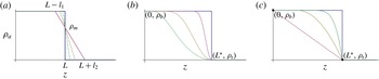
(a) A CLC sequence of approximations crossing the step function at density
 ${\it\rho}_{m}$
(
 ${\it\rho}_{t}\leqslant {\it\rho}_{m}\leqslant {\it\rho}_{b}$
), providing a class of profiles that regularize the jump conditions using the available exact linear solution. (b) A CSC sequence of step approximations, giving an example of another class of profiles that smoothly extend the regularizations of the jump conditions via the Gronwall estimates. (c) Two-layer (thick) and linear (dotted), quadratic (dashed) and quintic (dot-dashed) density profiles decreasing from
 ${\it\rho}_{b}$
to
 ${\it\rho}_{t}$
within distance
 $L^{\ast }$
. Profiles shown in (b,c) both depict examples of hatted densities which belong to the class of functions given in (2.45).

The jump conditions in § 2.5 most simply follow by approaching the step-function limit with a family of CLC profiles (see figure 2
a), generalized to intersect the limiting step function at any density
 ${\it\rho}_{m}$
,
 ${\it\rho}_{t}\leqslant {\it\rho}_{m}\leqslant {\it\rho}_{b}$
, by constructing the CLC ambient density function with
 ${\it\rho}_{a}(L^{\ast })={\it\rho}_{m}$
,
 $$\begin{eqnarray}{\it\rho}_{a}(z)=\left\{\begin{array}{@{}ll@{}}\displaystyle {\it\rho}_{b}, & z\in [0,L^{\ast }-l_{1}],\\ \displaystyle {\it\rho}_{b}-({\it\rho}_{b}-{\it\rho}_{t})(z-L^{\ast }+l_{1})/(l_{1}+l_{2}), & z\in [L^{\ast }-l_{1},L^{\ast }+l_{2}],\\ \displaystyle {\it\rho}_{t}, & z\in [L^{\ast }+l_{2},\infty ).\end{array}\right.\end{eqnarray}$$
The identity
 $$\begin{eqnarray}z(B_{2})-z(B_{1})=\int _{B_{2}}^{B_{1}}\frac{1}{N^{2}}\left[Q_{1}^{2}+4{\it\alpha}\int _{r}^{B_{1}}\left(\frac{M_{1}}{N^{8}}+\frac{2g{\it\lambda}^{2}}{N^{10}}(B_{1}^{2}-s^{2})\right)^{1/4}\text{d}s\right]^{-1/2}\text{d}r\end{eqnarray}$$
follows from (2.38), and, insisting on
 $z(B_{2})=L^{\ast }+l_{2}$
and
 $z(B_{1})=L^{\ast }-l_{1}$
(implicitly select values of
 $B_{1}$
,
 $B_{2}$
,
 $Q_{1}$
and
 $M_{1}$
), one can define
 $l\equiv l_{1}+l_{2}=z(B_{2})-z(B_{1})$
. Substituting
 $N^{2}=({\it\rho}_{b}-{\it\rho}_{t})/({\it\Lambda}{\it\rho}_{b}l)$
yields the identity
 $$\begin{eqnarray}1=\int _{B_{2}}^{B_{1}}\frac{{\it\Lambda}{\it\rho}_{b}}{({\it\rho}_{b}-{\it\rho}_{t})}\left[Q_{1}^{2}+4{\it\alpha}\int _{r}^{B_{1}}\left(\frac{M_{1}}{N^{8}}+\frac{2g{\it\lambda}^{2}}{N^{10}}(B_{1}^{2}-s^{2})\right)^{1/4}\text{d}s\right]^{-1/2}\text{d}r,\end{eqnarray}$$
and by taking the limit
 $l\rightarrow 0$
in (2.41) leads to (with standard bracket notation)
 $[B]_{L-}^{L+}=({\it\rho}_{t}-{\it\rho}_{b})Q(L^{-})/({\it\Lambda}{\it\rho}_{b})$
as
 $l\rightarrow 0$
, which justifies the jump condition (2.37). Continuity of
 $M$
follows from
 $2g{\it\lambda}^{2}([B]_{L-}^{L+})=N^{2}([M]_{L-}^{L+})$
as
 $l\rightarrow 0$
(B 3); this forces
 $[M]_{L-}^{L+}=0$
, as the left-hand side is non-zero. A similar argument (B 5) shows that
 $Q$
is continuous across the layer, which verifies continuity of
 $w=\sqrt{M}/Q$
.
2.5.2. Smooth approximation of step density jumps
Next, we further generalize the derivation of jump conditions by considering a family of CSC profiles limiting to a step (figure 2 b),
 $$\begin{eqnarray}{\it\rho}_{a}(z;z_{i})=\left\{\begin{array}{@{}ll@{}}\displaystyle {\it\rho}_{b}, & z\in [0,z_{i}],\\ \displaystyle {\it\rho}_{b}-({\it\rho}_{b}-{\it\rho}_{t})f_{s}(z), & z\in [z_{i},L^{\ast }],\\ \displaystyle {\it\rho}_{t}, & z\in [L^{\ast },\infty ),\end{array}\right.\end{eqnarray}$$
where
 $f_{s}$
is a smooth function with
 $f_{s}(z_{i})=0$
and
 $f_{s}(L^{\ast })=1$
for some
 $z_{i}<L^{\ast }$
. We study
 ${\it\beta}(z;z_{i})$
for (2.2) using
 ${\it\rho}_{a}(z;z_{i})$
. Integrating the
 ${\it\beta}$
equation starting from
 $z_{i}$
, and noting that
 $q$
is increasing with
 ${\it\beta}={\it\beta}_{0}$
in
 $[0,z_{i}]$
, it follows that
 $$\begin{eqnarray}{\it\beta}(L^{\ast };z_{i})={\it\beta}_{0}-\int _{z_{i}}^{L^{\ast }}\frac{|{\it\rho}_{a}^{\prime }|}{{\it\Lambda}{\it\rho}_{b}}q\,\text{d}s<{\it\beta}_{0}-q(z_{i})\int _{z_{i}}^{L^{\ast }}\frac{|{\it\rho}_{a}^{\prime }|}{{\it\Lambda}{\it\rho}_{b}}\,\text{d}s<{\it\beta}_{0}-q(z_{i})\frac{{\it\rho}_{b}-{\it\rho}_{t}}{{\it\Lambda}{\it\rho}_{b}}.\end{eqnarray}$$
Hence
 $$\begin{eqnarray}{\it\beta}_{0}-q(z_{i})\frac{{\it\rho}_{b}-{\it\rho}_{t}}{{\it\Lambda}{\it\rho}_{b}}>{\it\beta}(L^{\ast };z_{i})>B({L^{\ast }}^{+}),\end{eqnarray}$$
where the lower bound is provided in § 2.6. Since
 $q=Q_{h}$
(defined in (2.17)), sending
 $z_{i}\rightarrow L^{\ast }$
recovers (2.37).
As we shall see in § 4.5, the estimates we have established above allow us to provide rigorous bounds on trapping heights of jets/plumes in realistic applications.
2.6. Optimal mixing profile and lower bound for trapping height
Deriving exact solutions to the MTT system (2.2) with arbitrary stratified density profiles is challenging. However, by using the exact solution (2.34) in Gronwall-like estimates for the general system, we next establish optimal mixing properties for a broad class of density profiles, namely those that can be written as
 $$\begin{eqnarray}\hat{{\it\rho}}_{a}(z)={\it\rho}_{b}+({\it\rho}_{t}-{\it\rho}_{b})f(z),\quad \text{with }f(0)=0,~f(z)=1\quad \text{for }z\geqslant L^{\ast },\end{eqnarray}$$
where
 $f$
, in contrast with
 $f_{s}$
used above, is a continuously differentiable monotonically increasing function which may match non-smoothly to the constant-density top and bottom states. The reference two-layer step profile strictly dominates this class (see figure 2
c). For ease of comparison with system (2.35) and its jump conditions (2.37), we rewrite (2.2) for the general profiles by denoting the dependent variables with hats,
 $$\begin{eqnarray}\hat{Q}^{\prime }=2{\it\alpha}\hat{M}^{1/4},\quad \hat{M}^{\prime }=4g{\it\lambda}^{2}\hat{Q}\hat{B},\quad \hat{B}^{\prime }=-({\it\rho}_{b}-{\it\rho}_{t})f^{\prime }(z)\hat{Q}/({\it\rho}_{b}{\it\Lambda}),\end{eqnarray}$$
with the same positive initial data (2.36).
The goal is to show
 $\hat{B}(L^{\ast })>0\equiv B({L^{\ast }}^{+})$
, i.e. the buoyancy fluxes of all profiles in the ‘hat class’ are positive at
 $z=L^{\ast }$
, which would lead to escaping solutions for (2.46). In § 2.2 we showed that
 $\hat{Q}\leqslant Q_{h}=Q$
and
 $\hat{M}\leqslant M_{h}=M$
for
 $z\in (0,\min \{L^{\ast },\hat{z}_{s}\})$
since
 $B=B_{0}$
for
 $z\in [0,L^{\ast })$
, where
 $\hat{M}(\hat{z}_{s})=0$
. Next we show that
 $\hat{z}_{ne}>L^{\ast }$
where
 $\hat{B}(\hat{z}_{ne})=0$
. Now suppose by contradiction that
 $\hat{z}_{ne}\leqslant L^{\ast }$
. The fact that
 $\hat{M}$
attains its maximum value at
 $\hat{z}_{ne}$
yields
 $\hat{z}_{ne}<\hat{z}_{s}$
(
 $\hat{z}_{ne}\neq \hat{z}_{s}$
since
 $\hat{M}(\hat{z}_{ne})>M_{0}>0$
), and hence
 $Q\geqslant \hat{Q}$
in
 $(0,\hat{z}_{ne}]$
. Since
 $\hat{Q}$
and
 $Q$
are increasing, the estimate
 $$\begin{eqnarray}\int _{0}^{\hat{z}_{ne}}f^{\prime }\hat{Q}\,\text{d}z<\hat{Q}(\hat{z}_{ne})f(\hat{z}_{ne})\leqslant Q(\hat{z}_{ne})f(\hat{z}_{ne})\leqslant Q(\hat{z}_{ne})\end{eqnarray}$$
contradicts the assumption
 $\hat{z}_{ne}\leqslant L^{\ast }$
,
 $$\begin{eqnarray}0=\hat{B}(\hat{z}_{ne})>B_{0}-\frac{{\it\rho}_{b}-{\it\rho}_{t}}{{\it\rho}_{b}{\it\Lambda}}Q(\hat{z}_{ne})\geqslant B_{0}-\frac{{\it\rho}_{b}-{\it\rho}_{t}}{{\it\rho}_{b}{\it\Lambda}}Q({L^{\ast }}^{-})=B({L^{\ast }}^{+})=0,\end{eqnarray}$$
so that it must be
 $\hat{z}_{ne}>L^{\ast }$
. Since
 $\hat{B}$
is decreasing,
 $\hat{B}(L^{\ast })>\hat{B}(\hat{z}_{ne})=0$
, which completes the proof. Note that the first inequality in (2.47) is strict because equality holds only if
 $\hat{Q}$
is constant in
 $[0,\hat{z}_{ne}]$
. Furthermore, since
 $z_{s}>z_{ne}>L^{\ast }$
, the solution to (2.46) exists in the range
 $[0,L^{\ast }]$
.
In conclusion, the above argument proves that the two-layer profile is the best mixer since
 $\hat{Q}>0$
implies
 $\hat{{\it\theta}}(L^{\ast })>0$
so that
 $\hat{{\it\rho}}_{j}(L^{\ast })<{\it\rho}_{t}={\it\rho}_{j}({L^{\ast }}^{+})$
. Compared to the step stratification, the jet density in any stratification of the continuous class described above cannot exceed
 ${\it\rho}_{t}$
, i.e. the jet cannot be neutrally buoyant before
 $L^{\ast }$
, and hence keeps rising due to positive buoyancy after passing through a continuous density transition in this class. We remark that this optimal property extends to density profiles with steps located at shorter distances
 $L<L^{\ast }$
, since steps maximize the density increment after the jump, as follows from the Gronwall estimates above, rewritten for density,
 $$\begin{eqnarray}\displaystyle \hat{{\it\rho}}_{j}(L)={\it\rho}_{t}-{\it\rho}_{b}\hat{{\it\theta}}(L)={\it\rho}_{t}-{\it\rho}_{b}\hat{B}(L)/\hat{Q}(L)<{\it\rho}_{t}-{\it\rho}_{b}B(L^{+})/Q(L^{+})\equiv {\it\rho}_{j}(L^{+}), & & \displaystyle\end{eqnarray}$$
where the existence of the continuous hatted system is guaranteed by positivity of
 $\hat{B}$
at lengths shorter than critical.
It is worth noting that the system of differential equations given in (2.46), with density profiles in the class defined by (2.45), will enjoy global existence provided the initial distance between the jet and the transition point is less than or equal to
 $L^{\ast }$
(i.e. the jet nozzle locations,
 $z_{jet}$
, positioned at
 $z_{jet}\geqslant 0$
). This follows from the proof of optimality above, since the buoyancy is conserved in the top layer. However, this property clearly does not extend to jet nozzle locations with
 $z_{jet}<0$
, as the asymptotic results for constant-linear density profiles presented in appendix C rigorously document. Consequently, for the results obtained in this paper regarding the critical height and optimality for jets positioned with
 $z_{jet}\geqslant 0$
(the primary focus here), the plume height will diverge.
Further comments are in order for propagation distances not equal to
 $L^{\ast }$
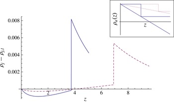
. Surprising, non-intuitive behaviour originates in the Gaussian closure from the weakest initial mixing occurring in homogeneous environments as compared to that associated with any stable stratification. As a result, if the distance travelled by the mixing jet does not sample the complete range of ambient densities, the optimal mixer is indeterminate. For example, figure 3 depicts the difference between the evolving jet density in homogeneous and in linear stratifications, with the jet nozzle positioned at the critical distance,
 $L^{\ast }$
: for short distances, the linear stratification is a better mixer than the two-layer case, whereas for longer distances this mixing property switches. For the nozzle positioned at distances
 $L$
larger than
 $L^{\ast }$
, similar behaviour can be observed numerically, with one additional complication arising from the possible loss of existence,
 $z_{s}\in (0,L)$
, in the limit of large
 $L$
(before the full range of ambient densities is sampled). For example, in the case of linear stratification, for large distances
 $L$
, direct mathematical analysis of the exact quadrature (2.38) indeed shows that the singularity height
 $z_{s}$
occurs within this range; see appendix C. Attempts to apply Gronwall-like estimates for general stratifications have not yet succeeded in extending the rigorous characterization of the optimal mixer in this regime.
Numerically computed jet density difference
 ${\it\rho}_{j}-{\it\rho}_{j,l}$
between two-layer and its linear stratification counterpart versus distance from the nozzle, with jump location at
 $L^{\ast }$
. Parameters are:
 ${\it\rho}_{b}=1.057~\text{g}~\text{cm}^{-3}$
,
 ${\it\rho}_{t}=1.045~\text{g}~\text{cm}^{-3}$
(solid),
 ${\it\rho}_{t}=1.05~\text{g}~\text{cm}^{-3}$
(dashed). Curves terminate at neutral buoyancy position of each linear profile. Inset shows the step and linear ambient density profiles for each parametric choice.

Some of the peculiar initial mixing properties for the Gaussian plume closure can be immediately seen from the estimate
 $$\begin{eqnarray}\bar{{\it\rho}_{j}}^{\prime }(0)=2{\it\alpha}M_{0}^{1/4}{\it\theta}_{0}{\it\rho}_{b}/Q_{0}-{\it\rho}_{a}^{\prime }(0)/{\it\Lambda}>2{\it\alpha}M_{0}^{1/4}{\it\theta}_{0}{\it\rho}_{b}/Q_{0}={\it\rho}_{j}^{\prime }(0),\end{eqnarray}$$
where
 $\bar{{\it\rho}_{j}}$
and
 ${\it\rho}_{j}$
are the jet densities in a stably stratified and sharply stratified environment, respectively. Figure 3 illustrates this initial behaviour, and shows the switching to optimality of the two-layer model at larger jet travel distances: the transition can occur well before the critical distance
 $L^{\ast }$
(solid curve), or right at the critical distance (dotted).
While the Gaussian plume closure model admits this peculiarity, for which the non-constant background density profile is initially a better mixer than the constant background, the top-hat closure model possesses a strong, pointwise ordering result which we now prove. Specifically, solutions of the top-hat closure model (denoted by the subscript
 $(\cdot )_{T}$
),
 $$\begin{eqnarray}q_{T}^{\prime }=2{\it\alpha}m_{T}^{1/4},\quad m_{T}^{\prime }=2gq_{T}{\it\beta}_{T},\quad {\it\beta}_{T}^{\prime }={\it\rho}_{a}^{\prime }q_{T}/{\it\rho}_{b},\end{eqnarray}$$
with an arbitrary background density profile always exhibit less mixing than their two-layer ambient density profile counterparts,
 $$\begin{eqnarray}{\it\rho}_{j,T}>\hat{{\it\rho}}_{j,T},\quad \text{for any }z>0.\end{eqnarray}$$
Here, we have followed the hatted and non-hatted convention defined above to refer to variable density with profile defined in (2.45) and piecewise-constant profiles, respectively. We will further follow this and letter capitalization conventions as before for the transformed variables
 $Q_{T}$
,
 $M_{T}$
and
 $B_{T}$
. Note that the initial conditions for the top-hat closure use the original physical initial conditions, without needing to rescale them to match mean fluxes, etc., as was required within the Gaussian closure model. From (2.51), it can be seen that
 $B_{T}=B_{0}$
for
 $z\in [0,L)$
, that is,
 $Q_{T}({\it\rho}_{b}-{\it\rho}_{j,T})=Q_{0}({\it\rho}_{b}-{\it\rho}_{j,T}^{0})$
; solving for
 ${\it\rho}_{j,T}$
gives
 $$\begin{eqnarray}{\it\rho}_{j,T}={\it\rho}_{b}-\frac{Q_{0}}{Q_{T}}({\it\rho}_{b}-{\it\rho}_{j}(0)).\end{eqnarray}$$
On the other hand, since
 $\hat{B}_{T}=B_{0}+{\it\theta}_{f}\int _{0}^{z}f^{\prime }\hat{Q}_{T}\,\text{d}s$
, multiply by
 ${\it\rho}_{b}$
on both sides to obtain
 $\hat{Q}_{T}(\hat{{\it\rho}}_{a}-\hat{{\it\rho}}_{j,T})=Q_{0}({\it\rho}_{b}-{\it\rho}_{j}(0))+({\it\rho}_{t}-{\it\rho}_{b})\int _{0}^{z}f^{\prime }\hat{Q}\,\text{d}s$
, so that
 $$\begin{eqnarray}\hat{{\it\rho}}_{j,T}=\hat{{\it\rho}}_{a}-\frac{Q_{0}}{\hat{Q}_{T}}({\it\rho}_{b}-{\it\rho}_{j}(0))+\frac{{\it\rho}_{b}-{\it\rho}_{t}}{\hat{Q}_{T}}\int _{0}^{z}\hat{Q}_{T}f^{\prime }\,\text{d}s.\end{eqnarray}$$
Taking the difference of (2.53) and (2.54) results in
 $$\begin{eqnarray}{\it\rho}_{j,T}-\hat{{\it\rho}}_{j,T}=Q_{0}({\it\rho}_{b}-{\it\rho}_{j}(0))\left(\frac{1}{\hat{Q}_{T}}-\frac{1}{Q_{T}}\right)+({\it\rho}_{b}-\hat{{\it\rho}}_{a})+\frac{{\it\rho}_{t}-{\it\rho}_{b}}{\hat{Q}_{T}}\int _{0}^{z}\hat{Q}_{T}f^{\prime }\,\text{d}s\geqslant 0,\end{eqnarray}$$
since the first term on the right-hand side is positive from the estimates in § 2.2, and the last two terms add up to be positive by the estimate
 $$\begin{eqnarray}\displaystyle ({\it\rho}_{b}-\hat{{\it\rho}}_{a})+\frac{{\it\rho}_{t}-{\it\rho}_{b}}{\hat{Q}_{T}}\int _{0}^{z}\hat{Q}_{T}f^{\prime }\,\text{d}s & = & \displaystyle ({\it\rho}_{b}-{\it\rho}_{t})f+\frac{{\it\rho}_{t}-{\it\rho}_{b}}{\hat{Q}_{T}}\int _{0}^{z}\hat{Q}_{T}f^{\prime }\,\text{d}s\nonumber\\ \displaystyle & = & \displaystyle \frac{{\it\rho}_{b}-{\it\rho}_{t}}{\hat{Q}_{T}}\left(\int _{0}^{z}f\hat{Q}_{T}^{\prime }\,\text{d}s\right)\geqslant 0.\end{eqnarray}$$
Lastly, a peculiarity arising in the Gaussian closure is that the density jump across the step is
 $[{\it\rho}_{j}]_{-}^{+}=({\it\rho}_{t}-{\it\rho}_{b})/{\it\lambda}^{2}$
, which is independent of the initial jet density, making possible a zero critical distance. To see this, assume that
 ${\it\rho}_{b}<(1+{\it\lambda}^{2}){\it\rho}_{t}$
and
 ${\it\rho}_{j}(0)>{\it\rho}_{t}+({\it\rho}_{t}-{\it\rho}_{b})/{\it\lambda}^{2}$
; the jump condition
 ${\it\rho}_{j}(L^{+})>{\it\rho}_{t}$
(guaranteeing trapping) is satisfied for any
 $L>0$
, and hence
 $L^{\ast }=0$
. Note that this does not occur in top-hat profiles:
 ${\it\rho}_{j}$
is continuous so that
 $L^{\ast }=L_{m}^{\ast }\geqslant 0$
. We remark that, for profiles not strictly dominated by a reference two-layer step stratification, additional complications may arise and will be explored in future work.
3. Miscible buoyant jet experiments
Here we describe the set-up of our experimental methodology for measuring turbulent buoyant jets in stratified background ambient density profiles. In all our experiments, jets were pumped vertically from below the fluid density transition in a Plexiglas tank of dimension 72.4 cm
 $\times$
56 cm
 $\times$
80 cm (
 $W\times D\times H$
). This tank was filled halfway with a salt-water solution of density
 ${\it\rho}_{b}$
. This density is measured (indirectly) by using WTW Cond 197i and Orion 550A conductivity meters with a WTW Tetracon 325 conductivity probe with a cell constant of
 $0.475\pm 1.5\,\%$
. A second salt-water solution of density
 ${\it\rho}_{t}$
 $({\it\rho}_{t}<{\it\rho}_{b})$
was mixed and poured slowly through a diffuser into the tank in order to minimize mixing between the fluid being poured and the fluid already in the tank. Pouring took approximately 45–60 min, creating sharp density transitions of thickness between 1.45 and 3.15 cm. All data presented here are constrained to have the density difference
 ${\it\rho}_{b}-{\it\rho}_{t}\simeq 0.012\pm 0.0004~\text{g}~\text{cm}^{-3}$
. A jet nozzle (of radius 0.4572 cm) located in the tank was attached to a reservoir of fresh water. The positions of the jet nozzle and of the conductivity probe were zeroed using a levelled laser, and the distances between the jet nozzle and respective heights of the 90 % (smaller distance,
 $L90$
) and 10 % (larger distance,
 $L10$
) values of density differences were recorded. The 90 % data are presented in figure 5, as this is the location where the plume begins to experience the density transition. A three-way valve was employed to recirculate the fresh-water jet fluid through the reservoir to minimize undesirable bubble injection. A gear pump (Cole-Parmer Gear Pump Drive 75211-10 with a Micropump Gear Pump O/C GJ-N25.PF15A) created a jet, and a Cole-Parmer 94778-00 flow meter with a
 $+$
GF
 $+$
Signet 3-2100-1L adapter was used to adjust the volumetric flow rate fixed at
 $4.4~\text{ml}~\text{s}^{-1}$
(unless otherwise noted), yielding an entry Reynolds number
 $Re\simeq 1370$
. The three-way valve was opened to fire the jet into the tank for 15 s. The procedure was repeated adjusting the distance between the jet nozzle and the transition layer to window the critical escape/trap height to within 2–3 mm. Tanks were re-poured after no more than eight jets were fired. The values of the data for the critical length,
 $L_{e}^{\ast }$
, are taken to be the average of these two distances, the first being the distance between the nozzle and
 $L90$
(or
 $L10$
) for the case where the jet escapes, and the second being the distance between the nozzle and
 $L90$
(or
 $L10$
) for the case where the jet traps (these differ by at most 2–3 mm for our entire dataset, typically smaller than 1 mm).
A second set of experiments were performed to test the optimal mixing result presented in § 2.6. We considered two different density profiles: one with an effectively sharp density transition and a second, smoother profile satisfying the requirements for an element of the class defined in (2.45). These profiles were measured with the density probe. The sharp profile was prepared using the technique described above, with a sharp transition layer approximately 1.4 cm thick. (We note that by pouring the top layer a little faster, a layer of thickness slightly larger than 1.4 cm was produced due to the mixing associated with the pouring process; through selective suction of the mixed layer fluid, the layer thickness could be reduced for repeatable matching of the profiles.) The jets were carefully levelled to be fired vertically, and relative heights of conductivity probe and jet nozzle were determined using the method described in the first experiments.
A faster flow rate,
 $15~\text{ml}~\text{s}^{-1}$
, was required to access a longer critical distance needed to provide extra room for the smoother profile while keeping our density profile within the class for optimal mixing, defined above. The ambient fluid was re-poured for each trial, measuring the density profile to guarantee that the transition layer was reproducible to within millimetres (compared to the overall thickness of 1.4 cm). In both cases, each jet was positioned to have the same background bottom density value of
 $1.0572~\text{g}~\text{cm}^{-3}$
at the nozzle location, and the same top density of
 $1.0492~\text{g}~\text{cm}^{-3}$
. To be precise, we define the
 $L1$
height to be the height at which the background stratification is larger than the top density value by an amount equal to 1 % of the density difference between the top and bottom densities, and in both the sharp and smooth profiles this height
 $L1=11.2~\text{cm}$
above the nozzle. In this comparative study between sharp and smooth stratifications, this density difference between the top and bottom homogeneous regions was kept at
 $0.008~\text{g}~\text{cm}^{-3}$
, which is smaller than the one used in the first set of the experiments. This smaller density difference, combined with larger flow rate, yields a larger critical distance than the one measured above for our first detailed dataset. We remark that this larger distance was important for repeatability, as it gave extra flexibility when pouring the smoother profile (satisfying the conditions defining our class of density profiles expressed by (2.45)).
The second (smoother) density profile was poured using a two-bucket method, seeking to create an approximately linear transition sandwiched between two limiting values of the bottom and top constant-density fluid. In practice, switching to a constant-density fluid in the two-bucket method inevitably leads to a long stratification tail as the tank is filled. This tail will cross the originally sharp layer (and hence would not be within our class of density profiles in which optimality is established). To stay with our optimality class, the two-bucket pouring method is designed to run out of bottom fluid at a depth in between
 $L90$
and
 $L10$
so that the smoother profile matches the sharper profile at a depth
 $L1$
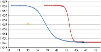
. This procedure yields two density profiles (see figure 4) which approximately satisfy the requirements needed to apply the optimal mixing results of the previous section. Lastly, the distance from
 $L1$
to the free surface in the sharp case is 20.8 cm, and in the smoother case is 14.6 cm. In each case, the total depth is 67 cm. For all the jets used in this set of experiments, the same pumping system was employed, and the flux monitored using a Proteus 800 Series NEMA 4 flow meter. The jet of the same density (in all experiments, dyed fresh water, density
 $0.9972\pm 0.0007~\text{g}~\text{cm}^{-3}$
, was used). A cap was positioned over each jet to prevent mixing between the background bottom fluid and the jet fluid, and carefully removed just prior to firing each jet. In this second set of experiments, the jet was then fired into the two different density profiles, each for 45 s, and subsequently observed to either escape or trap.
Effective two-layer stratification (red) and smoothed-out profile (blue) with two-bucket mixing method for intermediate layers. The two profiles have the same density (
 $1.0572~\text{g}~\text{cm}^{-3}$
) at the nozzle location (yellow circle) (jet behaviour is described in § 4) with the same constant density of
 $1.0492~\text{g}~\text{cm}^{-3}$
at the top. The black diamond is the location
 $L1$
defined in the text, and both jets are fired from the same distance between the yellow circle and
 $L1$
, 11.2 cm.

Miscible buoyant-jet trapping/escaping critical length versus
 ${\rm\Delta}\bar{{\it\rho}}$
, with layer thickness also shown for each experiment. (a) The
 $L10$
experimental data and theoretical curves
 $L_{m}^{\ast }$
, for different values of
 ${\it\lambda}$
and
 ${\it\alpha}$
. (b) The
 $L90$
experimental data with theoretical curve
 $L^{\ast }$
, for different values of
 ${\it\lambda}$
and
 ${\it\alpha}$
. Curves are theoretical predictions; and symbols are experimental data. Non-dimensional length scale normalized by nozzle radius
 $D$
(error bars based on instrumentation).

Lastly, a third set of jet experiments was conducted to explicitly assess the role that a lateral wall plays in modifying overall mixing and entrainments. In this experiment, the bottom-layer density was
 $1.0551\pm 0.0001~\text{g}~\text{cm}^{-3}$
and the top density was
 $1.0431\pm 0.0001~\text{g}~\text{cm}^{-3}$
using dyed fresh water, density
 $0.9972\pm 0.0007~\text{g}~\text{cm}^{-3}$
. One jet was fired from the tank centre, 36.2 and 28 cm away from the lateral walls and 31.6 cm above the bottom. A second jet was fired one nozzle diameter from a lateral wall and 28 cm from the back wall. Both cases were run at
 $15~\text{ml}~\text{s}^{-1}$
, and 12 cm below
 $L90$
; in the first case, the depth of
 $L90$
was 41.6 cm above the bottom, while in the second (wall) case, this depth was 40.1 cm. The layer thicknesses were, respectively, 2.3 cm and 3.9 cm. The jet apex heights in the upper fluid were then compared.
4. Validation of theoretical prediction with experimental and field observations
In this section, we focus on comparing the results of the theoretical predictions with a set of experiments and a field observations from the Deepwater Horizon oil spill in the Gulf of Mexico from 2010 (Joint Analysis Group 2011). We first compare experiments carried out to measure the critical distance in sharp stratification. Next we present an explicit demonstration of the optimal mixing result and also document a wall effect. Additionally, we explore the joint effects of nonlinear, local Richardson-number-dependent entrainment models and smooth but sharp density transitions. Lastly, we present an application of our analysis to the actual stratification that was measured in the Deepwater Horizon oil spill and obtain a mathematically rigorous lower bound for the depth of underwater plume formation.
4.1. Experimental measurements of the critical distance in sharp stratification and comparison with theory
The results of our experimental campaign are summarized in figure 5. The data for the experimentally measured critical distance,
 $L_{e}^{\ast }$
, are plotted as a function of the normalized density difference,
 ${\rm\Delta}\bar{{\it\rho}}$
. In figure 5(a),
 $L_{e}^{\ast }$
is represented as the distance between the jet nozzle and the depth of
 $L10$
, while in figure 5(b), this distance refers to
 $L90$
. Error bars are drawn with respect to the accuracy of the calibrated slider used to position the salinity probe. Also shown is the layer thickness (
 $L10$
–
 $L90$
) for each data point in the panels below (identical in both left and right cases). The theoretical curves are depicted based on the two-layer formula (2.29), using the two different models generated with the parameters
 $A^{\ast }$
and
 $A_{m}^{\ast }$
. The comparison shows the best agreement between the theoretical critical length and
 $L90$
data using
 $A^{\ast }$
(figure 5
b), and somewhat less quantitative agreement between the theoretical critical length and
 $L10$
data using
 $A_{m}^{\ast }$
(figure 5
a). This is not unexpected: since
 $A^{\ast }<A_{m}^{\ast }$
, the theoretical critical length
 $L^{\ast }$
is smaller than
 $L_{m}^{\ast }$
, and the model that does not incorporate the additional mixing due to the sharp layer should be expected to compare more favourably with the
 $L10$
data, while, conversely, the model accounting for sharp-layer mixing would do better with
 $L90$
experimental lengths. One interesting effect in this data concerns the role of the layer thickness. The clustering of layer thickness data in figure 5(c,d) around labels 12th–13th and 23rd–24th signifies two different thicknesses for essentially the same
 ${\rm\Delta}\bar{{\it\rho}}$
value (i.e. same initial jet, bottom and top densities). This allows a comparison between the experimentally measured critical lengths for different layer thickness: examination of
 $L_{e}^{\ast }$
in figure 5(a) shows that this quantity decreases with decreasing layer thickness (note that this effect is less noticeable in figure 5
b). This is essentially in agreement with the optimal mixing property: these data refer to increasingly sharper stratifications appear to limit to the theoretical optimal mixer depicted by the solid curve in figure 5(b); thus this particular data trend seems to be in agreement with our theoretical understanding.
Further, figure 5 depicts theoretical curves obtained using different constants
 ${\it\alpha}$
and
 ${\it\lambda}$
to test sensitivity on these parameters, starting with values that have been empirically established (see e.g. Fischer et al.
Reference Fischer, List, Koh, Imberger and Brooks1979). In figure 5(a,b) we have plotted the theoretical results using
 ${\it\lambda}=0.88$
and
 ${\it\lambda}=1.2$
(Kaminski, Tait & Carazzo Reference Kaminski, Tait and Carazzo2005). While in figure 5(a) varying
 ${\it\lambda}$
over these values shows strong variation in the predicted critical distance
 $L_{m}^{\ast }$
, the sensitivity is much weaker in figure 5(b) for the prediction employing the nonlinear jump conditions. In fact,
 $L^{\ast }$
is a monotonically decreasing function of
 ${\it\lambda}$
, and
 $L_{({\it\lambda}=1.2)}^{\ast }<L_{({\it\lambda}=0.88)}^{\ast }<1.075L_{({\it\lambda}=1.2)}^{\ast }$
, so that the critical distance is essentially insensitive to
 ${\it\lambda}$
in this range for figure 5(b), while agreeing well with the experimental data. The same lack of sensitivity cannot be claimed for the entrainment parameter
 ${\it\alpha}$
, as can be seen in figure 5, where both the plume entrainment value
 ${\it\alpha}=0.0833$
and intermediate (between jet and plume) entrainment value
 ${\it\alpha}=0.0684$
are compared, though again with figure 5(b) still showing less sensitivity. Further discussion of the role of entrainment modelling, particularly using the nonlinear, local Richardson-number-dependent entrainment law introduced by Priestley & Ball (Reference Priestley and Ball1955), as well as the effect of continuous stratification is reported below in § 4.3.
4.2. Demonstration of optimal mixer and a wall effect
We demonstrate experimentally the predicted optimal mixing by comparing the behaviour of turbulent buoyant jets in sharp versus smoother stratification profiles in our optimality class. The two profiles focused upon are depicted in figure 4. Recall, as described above in § 3, that in each case the jet is positioned to have the same background density value at the nozzle location and, by careful design, to have the same distance between the nozzle and
 $L1$
(11.2 cm). Our theory presented above in § 2.6 shows that, for any nozzle distance
 $L$
smaller than the theoretical critical distance, with
 $L\leqslant L^{\ast }$
, the sharp two-layer profile is the optimal mixer when compared to any profile in our class of density functions in (2.45). As such, to experimentally demonstrate this result, and to document that the smoother profile is a weaker mixer than the step-like profile, this distance is selected so that the jet in the sharper profile will be positioned just nearer than its critical distance, and the results compared. The jets are fired at the same flow rate of
 $15~\text{ml}~\text{s}^{-1}$
for the same duration of 45 s, and then turned off to make the comparison. In figure 6 the images of the two different cases are shown after the jets have been turned off and the tanks have settled. Figure 6(a) is the case of the smoother profile, and figure 6(b) is the case with the sharp profile. Clearly, in figure 6(a) the jet has escaped with the majority of the dyed (blue) fluid residing just below the free surface, while in figure 6(b) much of the fluid is trapped well below the free surface. Also, clearly, figure 6(a) has experienced less mixing than figure 6(b), and this demonstrates the optimality result. We comment that there is always concern for the role that the error bars play in making such sweeping statements, particularly in regards to making absolute statements about total mixing. We further examine this issue below in § 4.3.
Fresh-water dyed jets: (a) smooth ambient density stratification depicted in figure 4; (b) sharp density profile from same figure. Length scales are provided by the outer nozzle diameter of 0.657 cm as well as by metric rulers on the tank sides. Note the extra mixing associated with the sharp density profile.

It is interesting to note that figure 6(a,b) clearly exhibits a small accumulation of trapped jet fluid at the transition layer. This arises from the slow trickle of leaking jet fluid entering the tank after the jet is stopped, since this is done by closing a three-way valve that leaves some residual fluid in the feeding line, which then slowly leaks into the tank. An interesting question would be to consider why this fluid traps at all, given that it moves upwards through the bottom layer in an essentially laminar motion. We conjecture that the different physics of laminar enhanced diffusivity is at play in this regime, and this enhancement is responsible for the small volume of trapped fluid from the leaking lines seen in the experiments; we will explore this effect in future work.
Documentation of a wall effect. (a) The wall case apex reaches the free surface, while the centred jet (b) has apex well below the free surface. Snapshots are taking during the injection phase, and case (b) selected at the maximum jet penetration. See text for parameters.

We lastly observe that entrainment can be reduced by close proximity of the injection to walls through a third set of experiments, which agrees with the breakdown of the assumptions underlying the mathematical model in this case. We have tested proximity effects and found these to be negligible for nozzle locations more than 10 cm away from the bottom and lateral walls of our tank. An example of strong wall effect is shown in figure 7(a) where an overshoot of the jet fluid with respect to trapping for the same set-up as in figure 7(b) can be observed. The jet near the wall actually reaches the free surface, whereas the jet at the tank centre has apex height well below the free surface for all other similar experimental parameters. We discuss sensitivity issues regarding error bars in these fixed experimental parameters below in § 4.3.
We remark that while it may appear obvious that less background fluid entrainment is available to the jet in the case close to a lateral wall, we emphasize that such turbulent mixing is subtle: the wall also provides extra drag, which is non-trivial to quantify a priori if it increases or reduces overall mixing. For our cases studied, this clearly documents that the effect of the wall can reduce overall mixing. We also remark that this wall effect on entrainment distinguished our studies from studies such as those in slit geometries (Wallace & Sheff Reference Wallace and Sheff1987; Noh et al. Reference Noh, Fernando and Ching1992; Ching et al. Reference Ching, Fernando and Noh1993) for which the jet originated from a floor or a ceiling, which clearly would have similar effects as a vertical wall on entrainment.
4.3. Alternative entrainment modelling, and role of smooth stratifications
Here, we examine two natural improvements to our analytical theory, which will require some numerical assistance. The first targets improvement of entrainment modelling, and the second takes into account the finer structural details of the smooth background density stratification. Improvements to entrainment modelling within the MTT system have been proposed in the literature in the detailed functional form of the entrainment coefficient
 ${\it\alpha}$
(see e.g. Fischer et al.
Reference Fischer, List, Koh, Imberger and Brooks1979; Kaminski et al.
Reference Kaminski, Tait and Carazzo2005; Carazzo, Kaminski & Tait Reference Carazzo, Kaminski and Tait2006). We examine this issue in the context of our study.
We note that, for the experiment documenting the optimality of the two-layer stratification, the initial velocities are considerably higher than our full data above, and consequently the turbulent flow is closer to the jet-dominated limit initially. As such, to utilize the theoretical formulae to predict the critical distance, a different entrainment coefficient is needed. Applying our formula (2.29) with
 ${\it\alpha}={\it\alpha}_{p}\equiv 0.0833$
, the critical distance for these parameters is
 $L^{\ast }=6.06$
cm, whereas using the jet entrainment value of
 $0.0535$
produces a slightly more reasonable value of
 $L^{\ast }=9.29$
cm, recalling that the experimental critical distance in this case satisfies
 $L_{e}^{\ast }>7.8$
cm when measured between the nozzle and
 $L90$
for that case. To further improve the prediction in this intermediate regime between jet- or plume-dominated, a different entrainment model could be needed, as described in Fischer et al. (Reference Fischer, List, Koh, Imberger and Brooks1979).
The experiments conducted and the initial data selected in the MTT model have both
 $M_{0}$
and
 $B_{0}$
non-zero (and positive). (This further indicates that the behaviour of this study is neither a pure jet nor a pure plume, but a transition from buoyant jet to pure plume.) A key physical quantity that depicts this transition is the local Richardson number (Fischer et al.
Reference Fischer, List, Koh, Imberger and Brooks1979; Hunt & Kaye Reference Hunt and Kaye2005; Kaminski et al.
Reference Kaminski, Tait and Carazzo2005; Carazzo et al.
Reference Carazzo, Kaminski and Tait2006; Hunt & van den Bremer Reference Hunt and van den Bremer2010), defined as
 $$\begin{eqnarray}Ri(z)=\left[\frac{4\sqrt{2{\rm\pi}}{\it\lambda}^{2}}{1+{\it\lambda}^{2}}\left(\frac{gb{\it\theta}}{w^{2}}\right)\right]^{1/2}.\end{eqnarray}$$
Note that, as
 $w\rightarrow \infty$
,
 $Ri\rightarrow 0$
corresponding to a pure jet, while
 $w\rightarrow 0$
,
 $Ri\rightarrow \infty$
corresponds to a pure plume. It can be seen that in a homogeneous environment the far-field asymptotic relation yields a limiting Richardson number (independent of
 $z$
), which takes the value
 $\sqrt{16{\it\alpha}\sqrt{2{\rm\pi}}/(5({\it\lambda}^{2}+1))}\simeq 0.5131$
, when using the values
 ${\it\alpha}={\it\alpha}_{p}\equiv 0.0833$
and
 ${\it\lambda}=1.2$
. Experimentally, Wang & Law (Reference Wang and Law2002) measured the Richardson number ‘just after the jet flow became steady in clear ambient water’. Those authors claim the measurement to be taken within the asymptotic plume region, and the measured constant, called the plume Richardson number,
 $Ri_{p}$
, was reported to be
 $0.584$
(Wang & Law Reference Wang and Law2002). Similarly, a value of
 $0.557$
is reported in Fischer et al. (Reference Fischer, List, Koh, Imberger and Brooks1979). Priestley & Ball (Reference Priestley and Ball1955) report that
 ${\it\alpha}$
is proportional to the square of the local Richardson number, and hence a more appropriate entrainment function is
 $$\begin{eqnarray}{\it\alpha}={\it\alpha}_{j}-({\it\alpha}_{j}-{\it\alpha}_{p})\left(\frac{Ri(z)}{Ri_{p}}\right)^{2},\end{eqnarray}$$
where
 ${\it\alpha}_{j}\simeq 0.0535$
and
 ${\it\alpha}_{p}\simeq 0.0833$
.
Several interesting points emerge from our analysis. Firstly, the ratio of the local Richardson number to the constant-plume Richardson number,
 $Ri_{p}$
, should asymptote to unity at large distances for the model to be self-consistent. As just discussed, with a constant entrainment model, this constant is approximately
 $0.51$
, for the plume entrainment coefficient. It could be expected that the model in homogeneous ambient background fluid with nonlinear entrainment should match this, i.e. the asymptotic limit of the local Richardson number in the MTT system with nonlinear entrainment law (4.2) and a homogeneous ambient fluid would produce this self-consistent theoretical limit, and as such we will take
 $Ri_{p}\equiv 0.51$
for simplicity.
This limit does not appear amenable to an exact calculation, as the classical compendium of solvable differential equations by Kamke (Reference Kamke1944) indicates that this is not among the known analytically separable ordinary differential equations (ODEs). Hence the equivalent to the exact hypergeometric function used in our paper seems unavailable. One alternative is to assume power-law dependence of the evolving variables as a formal means to access this asymptotic large-distance limit. This indeed produces the same result and is derived in appendix D (numerical ODE integration, discussed next, additionally confirms that the limit of local Richardson number indeed approaches
 $\simeq 0.51$
for large distances).
Numerical ODE integration is required to make critical length predictions with the addition of nonlinear entrainment (as well as continuous stratification). We use both a fourth-order Runge–Kutta solver as well as the routine NDSolve in Mathematica for the simulations described next.
Critical height predictions with constant and variable entrainment coefficients,
 ${\it\alpha}$
. (a) The
 $L_{m}^{\ast }$
computed numerically and extended to variable entrainment in homogeneous background density. (b) The same for
 $L^{\ast }$
employing jump condition. Both panels compare with data and prediction from figure 5.

We next explore numerically the role of nonlinear entrainment in modifying the predictions of the critical length. Shown in figure 8 are numerical computations predicting the critical heights,
 $L_{m}^{\ast }$
and
 $L^{\ast }$
, but using the variable coefficient entrainment law in (4.2). In figure 8(a), the critical height is computed by solving in a homogeneous ambient with nonlinear entrainment for the height at which the jet density matches the top density. In figure 8(b), we do the same, except we formally impose density jump conditions, assuming all other variables are continuous (this property was rigorously established above but for the case of constant entrainment). These new predictions using variable entrainment increase the prediction of the critical length over those given with constant entrainment (which are also shown in figure 8). Also, figure 8(a,b) shows a tendency for the nonlinear entrainment prediction to approach those of constant entrainment as the normalized density difference
 ${\rm\Delta}\bar{{\it\rho}}$
increases to its maximum
 ${\rm\Delta}\bar{{\it\rho}}=1$
(in the limit
 ${\it\rho}_{j}\rightarrow 0$
,
 ${\rm\Delta}\bar{{\it\rho}}$
approaches unity). This property is consistent if the local Richardson number
 $Ri(z)$
approaches its limit
 $Ri_{p}$
faster with larger
 ${\rm\Delta}\bar{{\it\rho}}$
, which is observed in computations.
The critical length
 $L_{90}^{\ast }$
from the nozzle to
 $L90$
with background profile modelled by a complementary error function of thickness 2 cm: column 2 uses a constant entrainment coefficient
 ${\it\alpha}_{p}=0.0833$
; column 3 uses the nonlinear entrainment law. The theoretical step-based critical length
 $L^{\ast }$
: column 4 is with
 ${\it\alpha}_{p}$
; column 5, is the same as column 4 but with nonlinear entrainment law.

As in table 1, with but with thickness 0.2 cm.

Next, we explore the additional effects of including the detailed knowledge of the actual smooth background density to further improve the predictions of the observed
 $L_{e}^{\ast }$
. We mimic the step-like experimental density profile with an error function (the fixed-time solution of the heat equation between two limiting densities) with suitably selected parameters. We numerically integrate the MTT system with this continuous stratification and with or without nonlinear entrainment. For smooth transitions, the criterion used in these studies is to bracket the true critical length by monitoring the jet density as it evolves with respect to height. The numerical evidence of existence is demonstrated by the numerical solution being computable up to large distances (up to
 $z=10^{20}$
, using Mathematica’s NDSolve program, as well as our own Runge–Kutta fourth-order ODE solver, with smaller heights). Numerical evidence of breakdown is used to provide an upper bound of the critical length and a bisection strategy is used to narrow the gap between breakdown and existence until an accuracy of 0.1 % for the critical length is reached. Tables 1 and 2 present data comparing these effects. In table 1, the layer thickness is 2 cm, while in table 2 the layer thickness is 0.2 cm. In both tables, we label
 $L_{90}^{\ast }$
as the distance between the nozzle location and the position
 $L90$
of the smooth profile under the threshold criterion specified above and we indicate explicitly whether this was done with constant entrainment,
 ${\it\alpha}_{p}$
, or variable entrainment. Also listed in the tables are the critical heights calculated with both constant and variable entrainment in sharp stratification, as shown in figure 8. In table 1, for constant entrainment (
 ${\it\alpha}_{p}=0.0833$
), the role of a smooth background density yields critical lengths which are generally about 1 cm shorter than
 $L^{\ast }$
as well as approximately 1 cm below the
 $L90$
experimental data seen in figure 8(b). In contrast,
 $L_{90}^{\ast }$
with variable entrainment restores agreement with the data, and seems also to do the same with respect to the theoretical
 $L^{\ast }$
, which uses nonlinear jump conditions, but constant plume entrainment. Table 2 shows strong agreement with the theory for
 $L^{\ast }$
and
 $L_{90}^{\ast }$
with constant plume entrainment, as well as strong agreement between the variable entrainment
 $L_{90}^{\ast }$
with its variable entrainment
 $L^{\ast }$
counterpart. This, however, shows that the agreement in table 1 between
 $L^{\ast }$
and
 $L_{90}^{\ast }$
with variable entrainment and the experimental data has to be interpreted judiciously, given that it is a result of the particular stratification thickness length scale in both in silico and actual experiments. We remark that in actual experiments layer thicknesses smaller than 1.4 cm are not accessible with our current set-up, and hence table 2 does not have an experimental comparison.
We close this subsection with a remark about the use of nonlinear entrainment in stratified fluids. We are not aware of any reference that makes the case for applying such entrainment laws for the strong background density stratification which we have considered for most of our studies. Thus, as perhaps expected, the agreement observed above can be used to confirm that the most faithful model would be offered using both nonlinear entrainment and smooth density transitions. However, this set-up is hardly amenable to compact analytical predictions.
4.4. Sensitivity analysis within variable density and entrainment MTT system
Assessing the effectiveness of theoretically based conclusions in predicting actual experimental outcomes that are subject to error bar fluctuations is a fundamental question for any forecast. To this end, we now utilize the MTT model using both constant and variable entrainment with continuous background stratification to address sensitivity in its predictions as regards unavoidable small variations in experimental parameters, focusing primarily on effects of initial densities and layer thicknesses.
We first consider the optimal experiments presented above in § 4.2, and error bars in the initial jet densities. Recall that we presented a study documenting that the sharp stratification experiences greater mixing than the case with a carefully designed smooth background profile. A natural question would be to ask if that ordering extends over the entire error bar window of possible density values. We will use the full MTT system, varying initial parameters, to explore the theoretical sensitivity of the optimal mixing result. Assuming an initial jet density error bar of
 $0.0007~\text{g}~\text{cm}^{-3}$
as in our experiments, we integrate numerically system (2.1) with density profiles given by interpolation of the data presented in figure 4. Starting with the highest error bar limit, with an initial jet density of
 $0.9984~\text{g}~\text{cm}^{-3}$
, the numerical integration with variable entrainment predicts that the evolving jet density reaches the position
 $L1$
with a density value
 $1.04767~\text{g}~\text{cm}^{-3}$
in the sharp case and
 $1.03921~\text{g}~\text{cm}^{-3}$
in the smooth case, respectively. Next, with the lower initial jet density of
 $0.9977~\text{g}~\text{cm}^{-3}$
, the corresponding values are 1.04766 and
 $1.03911~\text{g}~\text{cm}^{-3}$
for the respective sharp and smooth cases. From these outcomes, it can be seen that the evolving density at
 $L1$
is essentially insensitive to this variation of initial jet density. Moreover, this also shows the effectiveness of the stratification sharpness in adding extra mixing right after the density step at
 $L1$
. Compared to the initial jet density variation of
 $0.0007~\text{g}~\text{cm}^{-3}$
, the additional mixing for the sharp case is approximately
 $0.0085~\text{g}~\text{cm}^{-3}$
. Also, the initial density variation is effectively suppressed in either sharp or smooth cases. These observations are just about the best that can be done within the simplification afforded by the MTT model and further confirms our optimal mixing conclusions in § 4.2 along with the theoretical ‘mixing quantum’ associated with the step that we predicted. Finally, we emphasize in all cases that these densities are consistent with the experimental outcomes depicted in figure 6: it can be noticed that the sharp case has red fluid spread throughout the entire top layer, in accordance with the weak escape for which density difference
 ${\it\rho}_{top}-{\it\rho}_{j}(L1)=0.0015~\text{g}~\text{cm}^{-3}$
. This is close to an order of magnitude smaller than in the smooth case, which experiences strong escape, in agreement with the model predicting
 ${\it\rho}_{top}-{\it\rho}_{j}(L1)=0.01~\text{g}~\text{cm}^{-3}$
. Further improvements could only be achieved by either an even more laborious experimental campaign and/or a fully resolved direct numerical simulation of the complete Navier–Stokes system.
Lastly, we perform a similar analysis applied to the case of the wall effect documented in § 4.2 in which the largest error fluctuation comes from the differences in the background layer thicknesses. The jet near the wall had a layer thickness scale of
 $3.9$
cm while the jet in the interior had a layer thickness scale of
 $2.3$
cm. In order to assess how these variations affect the jet mixing and hence support the conclusion that the role of the wall is dominant in reducing the overall mixing, we repeat the programme outlined above. This time, we run two cases, holding all parameters for each different jet as explicitly reported at the end of § 3; in particular, we assign the different layer thickness scales through the parameters of an error function density profile and compare the predicted apex heights. In both cases, the apex height was well below the free surface (using variable entrainment, with jet density initially
 $0.9977~\text{g}~\text{cm}^{-3}$
), reaching below the free surface
 $15.46$
cm in the thicker case, and
 $14.25$
cm in the sharp case, respectively. These are clear trapping cases, in contrast with the experimental observation for the jet near the wall (the thicker case actually penetrated further because it was initially a bit further from
 $L90$
than the sharper case, as reported above in § 3). We remark that the agreement for the apex height can only be qualitative for the MTT model with variable entrainment given by (4.2). As proposed by Kaminski et al. (Reference Kaminski, Tait and Carazzo2005) and Mehaddi et al. (Reference Mehaddi, Candelier and Vauquelin2013), the entrainment when negative buoyancy is reached should be modelled by a reduced entrainment coefficient possibly leading to a different higher apex than the one predicted with the original MTT system.
4.5. Application to the Deep Water Horizon (DWH) oil spill
The optimal mixing property of two-layer profiles can be used to provide rigorous, yet compact, closed-form bounds for the minimum distance that jets travel to reach a neutrally buoyant location in other classes of, not necessarily sharply stratified, density profiles. Interestingly, one can even consider, as an application, the very real case of the DWH oil spill in the Gulf of Mexico in 2010. Because of high temperatures, high velocities and the use of dispersants, the oil spill can be modelled as an emulsion (of several hydrocarbon species) able to mix with ambient fluid (for an experimental example of miscible emulsions, see e.g. Adalsteinsson et al. (Reference Adalsteinsson, Camassa, Harenberg, Lin, McLaughlin, Mertens, Reis, Schlieper and White2011)).
Local ocean stratifications (by potential density) in the DWH spill at different stations (green and blue) and concentration of hydrocarbons in the water column above the well head (red and black), all from NOAA Joint Analysis Group (2011). Critical distance
 $L^{\ast }$
as a function of
 ${\it\rho}_{t}$
(orange), varying from the surface density
 $\simeq 1.025~\text{g}~\text{cm}^{-3}$
to the maximum density at the well head
 $\simeq 1.02774~\text{g}~\text{cm}^{-3}$
, using the entrainment coefficient,
 ${\it\alpha}=0.0833$
. The horizontal dash-dotted line marks the intersection depth
 $L^{\ast }$
with ambient density.

By substituting the relevant parameters into our formula for
 $L^{\ast }$
, a lower bound for the trapping location can be established as follows. First, we set all relevant parameters in our model to match those made available through the oil spill field data report by Mariano et al. (Reference Mariano, Kourafalou, Srinivasan, Kang, Halliwell, Ryan and Roffer2011); thus the pipe radius is set to
 $r_{0}=20$
cm, the volumetric flow rate to
 $Q_{e}=1.2\times 10^{5}~\text{cm}^{3}~\text{s}^{-1}$
, the mean injection velocity to
 $w_{0}=Q_{e}/({\rm\pi}r_{0}^{2})~\text{cm}~\text{s}^{-1}$
, and the mean jet density to
 ${\it\rho}_{j}=0.85~\text{g}~\text{cm}^{-3}$
. In order to assign the top density
 ${\it\rho}_{t}$
required to apply our theory, we select a density from the range of values reported in ocean soundings from stations 20 and 25 reported by the NOAA Joint Analysis Group (2011). The bottom density
 ${\it\rho}_{b}$
is fixed to match that reported at the well head depth,
 ${\it\rho}_{b}=1.02774~\text{g}~\text{cm}^{-3}$
. By varying
 ${\it\rho}_{t}$
, we can construct the critical distances
 $L^{\ast }$
and plot them as a function of
 ${\it\rho}_{t}$
. In figure 9, the original density profile and fluorocarbon concentration (station 20 red, station 25 black) from the NOAA Joint Analysis Group (2011) report are reproduced, and the density profile interpolated using a quadratic law,
 ${\it\rho}(z)=1027.7427-5.31867\times 10^{-7}\,(z-100.943)^{2}~\text{kg}~\text{m}^{-3}$
, with vertical origin corresponding to the depth of
 $1600$
m as in the NOAA report’s graph. This interpolation is achieved by extracting the background density values at two locations, the well head depth at
 $1499.06$
m and the
 $800$
m depth point, by converting pixel values in the original NOAA report to depths using the length scales reported in the plot. The quadratic interpolation function is superimposed in the plot and depicted by a thin red curve. Also shown in figure 9 is the curve
 $L^{\ast }$
as a function of the density variable
 ${\it\rho}_{t}$
, decreasing from
 ${\it\rho}_{b}$
within the reported density range. The intersection of this curve
 $L^{\ast }({\it\rho}_{t})$
with the quadratic density profile
 ${\it\rho}(z)$
determines a key depth location, shown as the orange horizontal curve.
The construction of the lower-bound estimate for the trapping height is obtained by considering auxiliary density profiles as illustrated by figure 10(a–c). For a
 ${\it\rho}_{t}$
sufficiently small so as to be close to the initial jet density, the critical length
 $L^{\ast }$
for the first auxiliary step density profile
 ${\it\rho}_{aux1}$
, shown in figure 10(a), is small (in fact, approaching zero as
 ${\it\rho}_{t}\rightarrow {\it\rho}_{j}(0)$
) so that the height
 $L$
defined by
 ${\it\rho}(L)={\it\rho}_{t}$
is certainly larger than
 $L^{\ast }$
. The second auxiliary density profile
 ${\it\rho}_{aux2}$
, depicted in figure 10(a) and constructed piecewise by connecting a segment of
 ${\it\rho}(z)$
with the step at
 $L^{\ast }$
down to density value
 ${\it\rho}_{t}$
, lies within our comparison class of allowable profiles for optimal mixing. This assures that the jet density at
 $L^{\ast }$
is definitely smaller than
 ${\it\rho}(L^{\ast })$
, since, by our optimality proof,
 ${\it\rho}_{j}(L^{\ast })<{\it\rho}_{aux2}(L^{\ast })<{\it\rho}_{aux1}(L^{\ast })$
, where the first inequality follows from the mixing quantum of the second auxiliary profile step. Since
 ${\it\rho}(L^{\ast })>{\it\rho}(L)\equiv {\it\rho}_{t}$
by monotonicity of the background profile, the jet is still lighter than the background at
 $L^{\ast }$
and true trapping depth can only be above
 $L^{\ast }$
. This lower-bound height construction can clearly continue by varying
 ${\it\rho}_{t}>{\it\rho}_{j}(0)$
until the situation shown in figure 10(b) occurs, when
 $L^{\ast }=L$
. At this point we have the supremum of all lower bounds
 $L^{\ast }({\it\rho}_{t})$
, which provides our rigorous estimate of the trapping depth least upper bound (or greatest lower bound for trapping in terms of height above the well head) shown in figure 9 as the orange horizontal line. Figure 10(c) shows that this bound cannot be further improved, at least within the rigorous mathematical approach we have implemented, as the auxiliary function
 ${\it\rho}_{aux2}$
no longer belongs to the admissible comparison class of density profiles.
Auxiliary profiles used for the construction of the rigorous greatest lower bound for trapping height (distance above the well head). See text for details regarding the definition of the functions and scales. Vertical and horizontal scales are chosen in accordance to the NOAA Joint Analysis Group (2011) data.

When the procedure outlined above is applied to the actual NOAA data and the interpolation density
 ${\it\rho}(z)$
extracted from the data, the rigorous least upper bound on the trapping depth is
 $1302$
m. We observe that this depth is just below the depth of the largest fluorometry peak seen in the NOAA data, as shown in figure 9.
A simple non-rigorous prediction could of course be obtained based on treating the ambient ocean density as a constant, set at
 ${\it\rho}_{b}$
, and then finding the depth at which the evolving jet density matches the actual ocean density. This depth is
 $1242.97$
m, computed with the plume entrainment constant.
Of course, the full MTT model can also be numerically integrated with the quadratic density profile and trapping depths determined by matching the evolving jet density with that of the background (provided this occurs within the interpolation range below
 $800$
m depth). With a plume entrainment coefficient, this produces a trapping depth of
 $1232.12$
m. For comparison, running the same MTT model with the jet entrainment coefficient yields a trap depth of
 $1198.35$
m. Conversely, using the Richardson-number-dependent entrainment coefficient in the numerics yields a trap depth of
 $1228.99$
m. Hence, we can clearly see that the rigorous least upper bound on depth we provide is a reasonable and robust estimate, at least within the MTT theory in all these variants for entrainment parametrizations.
5. Discussion and conclusions
The MTT reduced models we have studied attempt to replace the complete jet dynamics by a finite set of collective variables for jet width, density and speed using an entrainment hypothesis. The rigorous mathematical results obtained here for both the top-hat and Gaussian profile closures concisely establish the two-layer stratification as being the optimal mixer over a class of suitably selected stable stratifications, despite complications arising in the Gaussian closure in which two-layer steps are not optimal for very short propagation distances. We remark that the two-layer stratified top-hat model performs poorly in predicting the critical distance data presented in figure 5, with that theory typically underpredicting the observed experimental critical distance,
 $L^{\ast }$
, by
 $30\,\%$
. This certainly justifies the need for Gaussian plume models after some initial short entry length. In future investigations, we hope to explore improvements to the model that address some of these complications by implementing more robust profile closure assumptions that merge an initial top-hat model transitioning to a Gaussian model over suitable length scales.
With our study of the MTT model in this work, prior jet/plume escaping criteria in the literature (Caulfield & Woods Reference Caulfield and Woods1998; Kaye & Scase Reference Kaye and Scase2011) are now proven rigorously. However, these criteria rely on a sufficiently large decay rate of the ambient density transition. Less was known about critical lengths in sharp stratifications. To the best of our knowledge, the analysis and data presented here are the first comprehensive study demonstrating a critical trapping phenomenon in these settings. In future work, we will attempt to extend our theory to applications beyond the ones described here, to include other relevant ocean settings, such as accumulations of ‘marine snow’ particulates at strong density stratification regions as reported by MacIntyre, Alldredge & Gotschalk (Reference MacIntyre, Alldredge and Gotschalk1995).
Acknowledgements
The authors thank C.-c. Caulfield for helpful discussions. The authors also thank the anonymous referee who suggested an asymptotic large-distance scaling relation between the critical distance and
 ${\rm\Delta}\bar{{\it\rho}}$
, which we developed in appendix C as a rigorous asymptotic result (C 2). We also extend our thanks to all the referees for their help in improving our exposition and suggesting expanding several points in the original manuscript. We thank the National Science Foundation for support through NSF RTG DMS-0502266, NSF RTG DMS-0943851, NSF RAPID CBET-1045653, NSF CMG ARC-1025523 and NSF DMS-1009750, and the Office of Naval Research for support through ONR DURIP N00014-09-1-0840. Z.L. acknowledges the support of Nation Science Foundation of China through grant 11201419. We thank D. Adalsteinsson for his visualization software DataTank. We also thank undergraduate research assistants, J. Reis, S. Harenberg, D. Vasco, W. Schlieper, M. Chancey, K. Ssekibakke, S. Lewis-Bevan, N. Perreau and C. Smith.
Appendix A. Derivation of critical distance with jump condition
Introducing new variables
 ${\it\Phi}=(w/{\it\theta})^{2}$
and
 ${\it\Psi}=1/{\it\theta}$
, (2.28a,b
) become
 $$\begin{eqnarray}\frac{\text{d}{\it\Phi}}{\text{d}z}=4g{\it\lambda}^{2}{\it\Psi},\quad \frac{\text{d}{\it\Psi}}{\text{d}z}=\left(\frac{2{\it\alpha}}{\sqrt{{\it\gamma}_{1}}}\right){\it\Phi}^{1/4}.\end{eqnarray}$$
Dividing the two equations and separating variables yields the conserved quantity
 $$\begin{eqnarray}{\it\Psi}^{2}=\left(\frac{4{\it\alpha}}{5\sqrt{{\it\gamma}_{1}}g{\it\lambda}^{2}}\right){\it\Phi}^{5/4}+A\quad \text{for }z<L.\end{eqnarray}$$
Imposing initial conditions determines
 $A={\it\theta}_{0}^{-2}-4{\it\alpha}\bar{w}_{0}^{2}/(5g{\it\lambda}^{2}\bar{b}_{0}{\it\theta}_{0}^{3})$
, where
 $\bar{w}_{0}$
,
 ${\it\theta}_{0}$
and
 $\bar{b}_{0}$
are the initial conditions for the system (2.28). By using the conserved quantity we immediately arrive at formula (2.34) for
 $z$
as a function of the density anomaly.
The critical distance
 $z^{\ast }$
separating escaping from trapping is selected by the upper limit of integration
 ${\it\Phi}_{f}$
in (2.34), which makes
 ${\it\gamma}_{2}=0$
. We use condition (2.37) and continuity of
 $b$
and
 $w$
to determine
 ${\it\Psi}(z^{\ast })={\it\Lambda}/{\it\theta}_{f}$
from
 $$\begin{eqnarray}{\it\gamma}_{2}={\it\gamma}_{1}-\lim _{z\rightarrow L^{-}}({\it\theta}_{f}/{\it\Lambda})b^{2}w(z)={\it\gamma}_{1}(1-({\it\theta}_{f}/{\it\Lambda}){\it\Psi}(z^{\ast }))=0,\end{eqnarray}$$
so that by (A 2) the critical upper limit of integration is
 $$\begin{eqnarray}{\it\Phi}_{f}=\left(\frac{{\it\Psi}(z^{\ast })^{2}-A}{a}\right)^{4/5}=\left(\frac{{\it\Lambda}^{2}{\it\rho}_{b}^{2}}{a({\it\rho}_{b}-{\it\rho}_{t})^{2}}-\frac{A}{a}\right)^{4/5}.\end{eqnarray}$$
(Note that the lower limit of integration in (2.34) is selected in terms of the initial conditions.)
Appendix B. Integral solution to linear ambient profile (2.38)
We denote the MTT model with linear ambient density profile as
 $$\begin{eqnarray}Q_{l}^{\prime }=2{\it\alpha}M_{l}^{1/4},\quad M_{l}^{\prime }=4g{\it\lambda}^{2}Q_{l}B_{l},\quad B_{l}^{\prime }=-N^{2}Q_{l},\end{eqnarray}$$
where the constant buoyancy (Brunt–Väisälä) frequency is
 $N^{2}=-{\it\rho}_{a}^{\prime }/({\it\Lambda}{\it\rho}_{b})$
, and initial conditions are defined as (2.36). Taking the ratio of (B 1b
) and (B 1c
) yields
 $$\begin{eqnarray}\frac{\text{d}B_{l}}{\text{d}M_{l}}=-\frac{N^{2}}{4g{\it\lambda}^{2}B_{l}},\end{eqnarray}$$
whence a conservation relation for
 $M_{l}$
and
 $B_{l}$
follows:
 $$\begin{eqnarray}2g{\it\lambda}^{2}B_{l}^{2}=-N^{2}M_{l}+C_{B}.\end{eqnarray}$$
Here the integration constant is positive,
 $C_{B}\equiv N^{2}M_{0}+2g{\it\lambda}^{2}B_{0}^{2}>0$
. By (B 3),
 $M_{l}=(C_{B}-2g{\it\lambda}^{2}B_{l}^{2})/N^{2}$
. Similarly, taking the ratio of (B 1a
) and (B 1c
) yields
 $$\begin{eqnarray}\frac{\text{d}Q_{l}}{\text{d}B_{l}}=-\frac{2{\it\alpha}M_{l}^{1/4}}{N^{2}Q_{l}}.\end{eqnarray}$$
By separation of variables,
 $$\begin{eqnarray}Q_{l}=\left(Q_{0}^{2}-\frac{4{\it\alpha}}{N^{5/2}}\int _{B_{0}}^{B_{l}}(N^{2}M_{0}+2g{\it\lambda}^{2}B_{0}^{2}-2g{\it\lambda}^{2}r^{2})^{1/4}\,\text{d}r\right)^{1/2},\end{eqnarray}$$
where
 $M_{l}$
is replaced by
 $B_{l}$
through (B 3). The exact inverse integral solution (2.38) then follows. Selecting
 $B_{l}=0$
yields the neutral buoyant height, whereas, by letting
 $M_{l}=0$
, relation (B 3) yields
 $B_{l}=-\sqrt{C_{B}/(2g{\it\lambda}^{2})}$
to give the apex height.
Appendix C. Long critical distance asymptotics
Using the relation
 $Q_{h}\sim C_{1}B_{0}^{1/3}z^{5/3}$
, a long-distance asymptotic relation for
 $L_{m}^{\ast }$
can be derived by solving for
 $z$
,
 $$\begin{eqnarray}Q{\it\theta}=Q(z)({\it\rho}_{b}-{\it\rho}_{j}(z))/{\it\rho}_{b}\sim C_{1}B_{0}^{1/3}z^{5/3}({\it\rho}_{b}-{\it\rho}_{j}(z))/{\it\rho}_{b}=B_{0},\end{eqnarray}$$
and imposing
 ${\it\rho}_{j}(z)={\it\rho}_{t}$
. This leads to the relation
 $$\begin{eqnarray}L_{m}^{\ast }=(Q_{0}/{\it\Lambda})^{2/5}(C_{1}{\it\theta}_{f})^{-3/5}({\rm\Delta}\bar{{\it\rho}})^{2/5},\end{eqnarray}$$
which can be viewed as another formula for the critical distance without any fitting parameter, and agrees well with large values of
 $L_{m}^{\ast }$
, since the asymptotic relation of
 $Q$
adapted here is valid only when the distance travelled is large enough. This asymptotic relation can also be derived by theoretically sending the density difference
 ${\it\rho}_{b}-{\it\rho}_{t}$
to zero, i.e.
 ${\it\theta}_{f}\rightarrow 0$
, since in that case
 $L_{m}^{\ast }\rightarrow \infty$
. Calculating the limit
 $\lim _{{\it\theta}_{f}\rightarrow 0}L_{m}^{\ast }/{\it\theta}_{f}^{-3/5}=(Q_{0}/{\it\Lambda})^{2/5}(C_{1})^{-3/5}({\rm\Delta}\bar{{\it\rho}})^{2/5}$
yields the relation above. A similar calculation on
 $L^{\ast }$
can also be done and yields the result
 $$\begin{eqnarray}L^{\ast }\sim {\it\Lambda}^{1/5}Q_{0}^{2/5}(C_{1}{\it\theta}_{f})^{-3/5}({\rm\Delta}\bar{{\it\rho}})^{2/5}\quad \text{as }{\it\theta}_{f}\rightarrow 0.\end{eqnarray}$$
We remark that neither of these two scaling relations, while properly asymptotic, fit our experimental data on account of the critical distances not being large enough for the parameters studied to reach this asymptotic regime.
Another interesting long-distance asymptotic relation focusing on a linear-constant profile is the following: for a pair of densities
 $({\it\rho}_{b},{\it\rho}_{t})$
, a linear-constant profile is characterized by a length scale
 $L$
,
 $$\begin{eqnarray}{\it\rho}_{a}(z)=\left\{\begin{array}{@{}ll@{}}\displaystyle {\it\rho}_{b}-({\it\rho}_{b}-{\it\rho}_{t})z/L, & z\in [0,L],\\ \displaystyle {\it\rho}_{t}, & z\in [L,\infty ).\end{array}\right.\end{eqnarray}$$
It can be shown by the optimal mixing result that
 $z_{ne}=\infty$
if
 $L\leqslant L^{\ast }$
. However, by studying the exact formula (2.38), one can show that
 $z_{s}\sim CL^{3/8}$
as
 $L\rightarrow \infty$
for some positive constant
 $C$
, i.e. the ordering
 $z_{ne}<z_{s}<L$
holds for
 $L$
large enough, and hence the plume will trap. We remark that this result agrees with the original similarity trap height scaling laws presented in Morton et al. (Reference Morton, Taylor and Turner1956), Caulfield & Woods (Reference Caulfield and Woods1998) and Woods (Reference Woods2010). In future studies, we will explore families of nonlinear density profiles sandwiched between these ‘linear-constant’ functions and step transitions. We conjecture that the breakdown point,
 $z_{s}$
, will exhibit scaling properties in the large-
 $L$
asymptotic limit, but these cases are complicated by similar competing effects such as those documented in figure 3. Candelier & Vauquelin (Reference Candelier and Vauquelin2012) presented a matched asymptotic expansion for the MTT in a homogeneous ambient density. We remark that their formulae when applied in a similar fashion for obtaining
 $L_{m}^{\ast }$
, when using the complete, uniformly valid expansion (for large/small Richardson number) would offer an alternative to our use of the exact hypergeometric integral. However, this does not seem to offer a substantial simplification unless use of the outer/inner solution alone can be justified. It would be interesting to try to extend this matched asymptotic analysis to more general density profiles as well as variable Richardson-number entrainment, where an exact solution is not available in homogeneous background.
Appendix D. Power-law asymptotic relation for variable coefficient entrainment
In a homogeneous background density profile, if the entrainment coefficient
 ${\it\alpha}$
in (2.1a
) is replaced by the entrainment law (4.2),
 $$\begin{eqnarray}{\it\alpha}={\it\alpha}_{j}-({\it\alpha}_{j}-{\it\alpha}_{p})\left(\frac{Ri(z)}{Ri_{p}}\right)^{2},\end{eqnarray}$$
among the power-law functional relationships, we will show below that the only ones consistent are
 $b$
,
 $w$
and
 ${\it\theta}$
given by
 $b\sim (6{\it\alpha}_{p}z/5)$
,
 $w\sim (25g{\it\lambda}^{2}B_{0}/24{\it\alpha}_{p}^{2})^{1/3}z^{-1/3}$
and
 ${\it\theta}\sim (625B_{0}^{2}/1944g{\it\lambda}^{2})^{1/3}z^{-5/3}$
. In fact, for these power laws, the local Richardson number approaches a limit
 $$\begin{eqnarray}\displaystyle Ri(z)\rightarrow Ri_{p}=\sqrt{16{\it\alpha}_{p}\sqrt{2{\rm\pi}}/(5({\it\lambda}^{2}+1))}\simeq 0.5131, & & \displaystyle\end{eqnarray}$$
when using the values
 ${\it\alpha}_{p}=0.0833$
and
 ${\it\lambda}=1.2$
, as
 $z\rightarrow \infty$
.
To establish this result, suppose
 $b\sim C_{b}z^{p_{b}}$
,
 $w\sim C_{w}z^{p_{w}}$
and
 ${\it\theta}\sim C_{{\it\theta}}z^{p_{{\it\theta}}}$
, as
 $z\rightarrow \infty$
. It follows that
 $Ri(z)\sim C_{Ri}z^{p_{b}+p_{{\it\theta}}-2p_{w}}$
, where
 $C_{b}$
,
 $C_{w}$
,
 $C_{{\it\theta}}$
and
 $C_{Ri}$
are constants, and
 $p_{b}$
,
 $p_{w}$
and
 $p_{{\it\theta}}$
are exponents. These exponents of
 $z$
in the MTT system (2.1) need to be balanced, and of the three possibilities evident from the volume equation,
 $$\begin{eqnarray}\displaystyle \frac{\text{d}(b^{2}w)}{\text{d}z}=2\left({\it\alpha}_{j}-({\it\alpha}_{j}-{\it\alpha}_{p})\left(\frac{Ri(z)}{Ri_{p}}\right)^{2}\right)bw, & & \displaystyle\end{eqnarray}$$
only the equality
 $p_{b}+p_{{\it\theta}}-2p_{w}=0$
is consistent with the system in a homogeneous background density. Under this condition, the exponent triplet is
 $(p_{b},p_{w},p_{{\it\theta}})=(1,-1/3,-5/3)$
. This relation also implies
 $Ri\rightarrow Ri_{p}$
as
 $z\rightarrow \infty$
.