Introduction
Reflectarray antennas (RAs) have attracted extensive research interest due to their low profile, high gain, lightweight structure, and ease of fabrication. Combining the advantages of parabolic reflectors and phased arrays, reflectarrays employ a spatial feed system instead of a complex feed network, effectively minimizing distribution losses while providing flexible beam-shaping capabilities through element-wise phase control [Reference Munson, Haddad and Hanlen1–Reference Ning, Zhu, Chu, Zou, Zhang and Li4]. These attributes make them excellent candidates for modern satellite communication, radar sensing, and wireless power transmission systems where compactness and efficiency are essential.
However, the operational bandwidth of conventional reflectarrays is typically narrow, mainly limited by the frequency-dependent reflection phase characteristics of individual elements [Reference Pozar5]. The phase response of most patch-type elements varies nonlinearly with frequency, resulting in phase errors across the aperture and degraded radiation performance. Achieving broadband operation therefore requires innovative unit-cell designs capable of maintaining linear phase variation and stable reflection amplitude over a wide frequency range.
Recent research has explored various strategies to mitigate the inherent bandwidth limitations of RAs. Adjusting the size, shape, and arrangement of reflective elements has proven effective in enhancing bandwidth performance. For example, wideband, tightly coupled dipole reflectarrays using three-dimensional (3D) elements placed in close proximity have been introduced [Reference Li, Tu, He, Zhang, Wong and Gao6, Reference Wu, Hu, Luo, Zhao, Jiang and Chen7]. This arrangement enhances inter-element coupling, thereby extending operational bandwidth. For instance, a tightly coupled reflectarray reported by Wu et al. [Reference Wu, Hu, Luo, Zhao, Jiang and Chen7] achieves an ultra-wide operating bandwidth of 90%. However, it significantly increases design complexity and manufacturing costs. Additionally, other studies [Reference Zhao, Fu, Li, Li and Hu8, Reference Min and Guo9] have adopted multi-resonant reflectarray elements that introduce supplementary resonances, enhancing phase linearity and broadening the frequency response. Despite these improvements, multi-resonant structures inherently add complexity to antenna designs. Alternatively, subwavelength unit cells enable multiple elements to be integrated within a half-wavelength spacing, thereby improving phase compensation accuracy and broadening the achievable bandwidth [Reference Min and Guo9–Reference Zhao, Wei, Shi and Zeng12]. Extending this concept, a 1-bit reconfigurable reflectarray based on polarization-rotating unit cells achieves a unit-cell bandwidth of about 30% and a corresponding 3-dB gain bandwidth exceeding 30% for a fixed beam state [Reference Luyen, Zhang, Booske and Behdad10]. Similarly, a dual-circularly-polarized multi-beam reflectarray employing a subwavelength shared-aperture configuration achieves a 3-dB gain bandwidth of approximately 20% in the Ka-band [Reference Zhang, Dai, Fu, Tang and Mi11], demonstrating the potential of subwavelength techniques for broadband multi-beam and dual-polarized applications. Another approach applies encoded metasurface theory to reflective surfaces. However, encoded reflective elements typically provide limited phase resolution, which can degrade radiation performance, reduce directivity, and lower aperture efficiency. Moreover, broadband operation may introduce frequency-dependent beam distortion, leading to beam squinting or pointing deviations and making it difficult to maintain stable radiation characteristics across a wide bandwidth. The C band is widely used in satellite communications due to its favorable propagation characteristics [Reference Jost, Wang, Perez-fontan and Fiebig13]. RAs have emerged as high-gain antennas for long-distance communications. Conventional parabolic reflector antennas are widely used for satellite links; however, small satellite platforms have limited payload capacity for bulky reflector antennas [Reference Kim, Hwang, Jeong, Lim, Park and Kim14]. In a reflectarray, each element controls the phase of the reflected wave to synthesize the desired radiation beam.
In this work, a novel double-layer RA employing subwavelength multi-resonant elements is proposed to achieve broadband performance in the C band. The design combines a dual-layer dielectric configuration with complementary resonant structures on separate layers to form triple-resonance characteristics. The upper layer employs circular-ring and curved delay-line elements, while the lower layer integrates Koch-fractal-inspired loops and cross-shaped patches to achieve wideband phase compensation. An ultra-wideband printed log-periodic dipole antenna (LPDA) serves as the feed, providing uniform amplitude distribution and reducing aperture blockage.
The remainder of this paper is organized as follows. The section on “Reflectarray element design” describes the design and operating mechanism of the proposed double-layer reflective unit. The section on “Scan parameter optimization” discusses the parameter optimization process and mutual-coupling analysis. The section on “Feed structure design” introduces the broadband LPDA feed design. The section on “Design of RA” presents the configuration of the complete reflectarray and its phase-compensation model. The section on “Design of RA” provides the simulated and measured results, followed by the conclusion in the section on “Conclusion”.
Reflectarray element design
To realize broadband operation with high phase stability, a multilayer subwavelength reflective element was developed. The configuration of the proposed unit cell is illustrated in Fig. 1. It consists of two stacked dielectric substrates (PTFE, ε r = 2.55) separated by an air gap. The upper substrate (thickness = 3 mm) and the lower substrate (thickness = 2 mm) are both printed with metallic patterns, while a continuous copper sheet on the bottom of the second layer serves as the ground plane. The unit-cell size is fixed at P = 16 mm, corresponding to approximately 0.33λ₀ at 6.2 GHz, thus ensuring subwavelength spacing to suppress grating lobes and maintain accurate phase control.
(a) Unit stereogram. (b) Unit side view. (c) Upper-layer unit structure composition. (d) Higher-frequency reflective elements. (e) Frequency-selective surface elements. (f) Lower-layer unit structure composition. (g) Medium-frequency reflective elements. (h) Low-frequency reflective elements.

Figure 1 Long description
The image consists of multiple sub-images labeled from (a) to (h). The sub-image (a) shows a unit stereogram of a multilayer structure with two stacked dielectric substrates separated by an air gap. The upper and lower substrates are printed with metallic patterns and a continuous copper sheet serves as the ground plane. Sub-image (b) provides a side view of the unit, indicating the thicknesses of the substrates and the air gap. Sub-image (c) illustrates the upper-layer unit structure composition with circular metallic patterns. Sub-image (d) depicts higher-frequency reflective elements with a circular design and labeled dimensions such as R subscript o and a. Sub-image (e) shows frequency selective surface elements with a circular pattern and dimensions labeled as W, F subscript r and r subscript i. Sub-image (f) presents the lower-layer unit structure composition with a cross-like metallic pattern. Sub-image (g) displays medium-frequency reflective elements with a cross pattern and dimensions labeled as a and g. Sub-image (h) illustrates low-frequency reflective elements with a simple cross pattern and dimensions labeled as E subscript s and g. The unit-cell size is fixed at P, ensuring subwavelength spacing to suppress grating lobes and maintain accurate phase control.
The upper layer incorporates an arc-shaped delay-line structure, designed to generate controllable phase variations by tuning the arc angle α from 0° to 170°, yielding a 340° phase-shift range at 6.2 GHz. On the lower dielectric substrate, a cross-shaped resonator and a Phoenix-type square-ring resonator are printed in a crossed configuration to realize additional resonances at 4.8 and 5.2 GHz, respectively. By combining these three structures, the unit cell achieves triple-resonant characteristics that effectively broaden the usable frequency range while maintaining smooth phase dispersion.
To optimize the reflection magnitude and phase response, full-wave simulations were performed under infinite periodic boundary conditions with Floquet-mode excitation. The reflection-phase curves demonstrate that the designed unit provides a continuous 360° phase range with reflection magnitude exceeding 0.9 across the entire band of interest. The optimized geometric parameters of the proposed element are summarized in Table 1.
Structural parameters of the proposed reflectarray element

Table 1 Long description
The table lists geometric parameters for a proposed reflectarray element, with all values given in millimeters. Fixed dimensions are P 16, h 2, h1 3, R1 6, a 1, b 6.7, and d 13. Two parameters are specified as adjustable ranges: c varies from 1 to 6.7, and g varies from 1 to 6.0. Among the fixed values, P is the largest and a is the smallest. The ranges indicate that c can span from very small up to the same size as b, while g spans a slightly smaller maximum. No performance outcomes are included, so the table supports geometry reference only and does not indicate how changes in c or g affect results.
Scan parameter optimization
The influence of the air-layer thickness between the two substrates on phase behavior was also investigated. As shown in Fig. 2, increasing the air gap from 1 mm to 5 mm produces a noticeable shift in the phase curve due to changes in the equivalent impedance. The optimal thickness of 3 mm was selected to achieve the best compromise between phase linearity and reflection stability.
The phase of the reflection coefficient of the element for different values of h 1. (a) Upper ring. (b) Koch fractal. (c) Cross unit.

Figure 2 Long description
The image contains three multi-line graphs labeled (a), (b) and (c), each plotting the phase of the reflection coefficient on the vertical axis in degrees, ranging from approximately negative 350 to positive 50, against a horizontal axis representing a swept parameter. Each graph contains three lines corresponding to air-layer thicknesses of 1 mm, 3 mm and 5 mm, as identified in the legend. The three lines are visually distinguished by different line styles and shading. Common structure across all three graphs: the vertical axis is labeled as phase in degrees and spans from approximately negative 350 to positive 50. The horizontal axis varies per panel as described below. The legend entries are labeled as h subscript 1 equals 1 mm, h subscript 1 equals 3 mm and h subscript 1 equals 5 mm. Graph (a) is labeled Upper Ring. The horizontal axis ranges from 0 to 100. All three lines begin near 0 degrees at the low end of the horizontal axis and transition sharply downward, reaching approximately negative 300 to negative 350 degrees toward the high end. The line for 1 mm transitions earliest, followed by 3 mm, then 5 mm, with the 5 mm line showing a noticeably later and steeper drop. The separation between lines is most visible in the mid-range of the horizontal axis. Graph (b) is labeled Koch fractal. The horizontal axis ranges from 0 to 7. The three lines again begin near 0 degrees at the low end and decline steeply. The transition region occurs between approximately 2 and 5 on the horizontal axis. The 1 mm line drops earliest, the 3 mm line drops at a mid-range position and the 5 mm line drops latest. End values for all three lines converge near negative 300 to negative 350 degrees. Graph (c) is labeled Cross unit. The horizontal axis ranges from 1.0 to 4.0. All three lines start near 0 degrees at 1.0 and decline steeply, reaching approximately negative 300 to negative 350 degrees by 4.0. The 1 mm line transitions at the lowest horizontal value, while the 5 mm line transitions at the highest horizontal value. The three lines are most separated in the range of approximately 1.5 to 3.0, then converge at the high end.
Mutual coupling between neighboring unit cells was further analyzed using two-element periodic models shown in Fig. 3. The results indicate that the bilayer configuration effectively isolates the two resonant surfaces, minimizing coupling effects and ensuring independent phase control. Moreover, the phase-shift responses under oblique incidence (θ, φ = 0°–45°) were examined, as shown in Figs 4 and 5. The phase deviations are maintained within ±5° over all tested incidence angles, thereby confirming the unit cell’s low angular sensitivity, which is a critical requirement for practical reflectarray applications.
Mutual coupling between two elements.

Figure 3 Long description
The image A showing (a) Reflected Phase (deg) The horizontal axis label is g (mm). The horizontal axis range is 1.0 to 6.0. The vertical axis label is Reflected Phase (deg). The vertical axis range is 0 to negative 450. Legend: c equals 1mm; c equals 3mm; c equals 5mm. Line identification by visual appearance: three solid lines. Data points as coordinate pairs. c equals 1mm: (1.0, negative 50), (2.0, negative 50), (3.0, negative 50), (3.5, negative 100), (4.0, negative 350), (4.5, negative 400), (5.0, negative 410), (6.0, negative 420) c equals 3mm: (1.0, negative 50), (2.0, negative 50), (3.0, negative 50), (3.5, negative 100), (4.0, negative 350), (4.5, negative 400), (5.0, negative 410), (6.0, negative 420) c equals 5mm: (1.0, negative 50), (2.0, negative 50), (3.0, negative 50), (3.5, negative 100), (4.0, negative 350), (4.5, negative 400), (5.0, negative 410), (6.0, negative 420) Key values and changes. All three series share the same listed coordinates. The largest change occurs between g equals 3.5 mm at negative 100 deg and g equals 4.0 mm at negative 350 deg. The lowest listed value is negative 420 deg at g equals 6.0 mm. The image B showing (b) Reflected Phase (deg) The horizontal axis label is c (mm). The horizontal axis range is 1 to 7. The vertical axis label is Reflected Phase (deg). The vertical axis range is 100 to negative 400. Legend: g equals 2mm; g equals 4mm; g equals 6mm. Line identification by visual appearance: three solid lines. Data points as coordinate pairs. g equals 2mm: (1, 0), (2, 0), (3, negative 20), (4, 0), (5, negative 200), (6, negative 350), (7, negative 350) g equals 4mm: (1, 0), (2, 0), (3, negative 20), (4, 0), (5, negative 200), (6, negative 350), (7, negative 350) g equals 6mm: (1, 0), (2, 0), (3, negative 20), (4, 0), (5, negative 200), (6, negative 350), (7, negative 350) Key values and changes. All three series share the same listed coordinates. The largest change occurs between c equals 4 mm at 0 deg and c equals 5 mm at negative 200 deg, followed by c equals 6 mm at negative 350 deg. The lowest listed value is negative 350 deg at c equals 6 mm and c equals 7 mm.
The phase of the reflection coefficient of the element for different incident angles theta. (a) Upper ring. (b) Koch fractal. (c) Cross unit.

Figure 4 Long description
The image A showing a multi-line line graph labeled (a) with the text Upper Ring. Horizontal axis label: Frequency (gigahertz). Horizontal axis range: 0.0 to 16.0. Vertical axis label: Phase (degree). Vertical axis range: 150 to negative 250. Legend entries: theta equals 0 degree; theta equals 15 degree; theta equals 30 degree; theta equals 45 degree. The four lines follow a similar shape: values near 150 degrees at low frequency, then a gradual decrease, then a steep drop, then a low plateau near negative 250 degrees at higher frequency. The steep drop occurs around the middle of the frequency range and the lines remain close to each other through most of the plot. The image B showing a multi-line line graph labeled (b) with the text Koch fractal. Horizontal axis label: Frequency (gigahertz). Horizontal axis range: 0.0 to 7.0. Vertical axis label: Phase (degree). Vertical axis range: 150 to negative 250. Legend entries: theta equals 0 degree; theta equals 15 degree; theta equals 30 degree; theta equals 45 degree. The four lines start near 150 degrees at low frequency, show small step-like decreases, then drop sharply to values near negative 250 degrees toward the higher end of the frequency range. The lines are closely grouped, with small separations visible during the mid-frequency steps. The image C showing a multi-line line graph labeled (c) with the text Cross unit. Horizontal axis label: Frequency (gigahertz). Horizontal axis range: 1.0 to 5.5. Vertical axis label: Phase (degree). Vertical axis range: 150 to negative 250. Legend entries: theta equals 0 degree; theta equals 15 degree; theta equals 30 degree; theta equals 45 degree. The four lines remain near 150 degrees at lower frequencies, then transition through a steep drop to values near negative 250 degrees, followed by a low plateau toward the highest frequencies. The lines overlap closely across most of the plot, with small differences visible around the transition region.
The phase of the reflection coefficient of the element for different incident angles phi. (a) Upper ring. (b) Koch fractal. (c) Cross unit.

Figure 5 Long description
The image contains three multi-line graphs labeled (a), (b) and (c), each comparing the phase of the reflection coefficient in degrees for different incident angles phi. The legend identifies five phi angles: phi equals 0 degree, phi equals 15 degree, phi equals 30 degree, phi equals 40 degree and phi equals 45 degree. In graph (a), the x-axis is labeled g (millimeter) ranging from 0 to 7 and the y-axis is labeled Phase (degree) ranging from 50 to negative 350. The lines show a steep decline in phase as g increases, with the phase leveling off around g equals 5 millimeters. The curves for different phi angles overlap closely, indicating similar behavior across angles. Graph (b) has the x-axis labeled g (millimeter) ranging from 0 to 100 and the y-axis labeled Phase (degree) ranging from 50 to negative 350. The phase decreases sharply as g increases, with notable leveling off around g equals 50 millimeters. The lines for different phi angles show slight variations but generally follow a similar trend. Graph (c) features the x-axis labeled g (millimeter) ranging from 0 to 5.5 and the y-axis labeled Phase (degree) ranging from 50 to negative 350. The phase drops significantly as g increases, leveling off around g equals 3 millimeters. The curves for different phi angles are closely aligned, showing minimal deviation. The lines are visually distinguished by color, allowing mapping from the legend to the curves. The graphs demonstrate consistent phase behavior across different g ranges and phi angles, highlighting the unit cell's low angular sensitivity and effective phase control.
Finally, the optimized amplitude and phase responses of the reflective element are presented in Fig. 6. The results show that the proposed multi-resonant structure provides a full 360° phase variation while maintaining a reflection magnitude close to 0 dB. Moreover, within the operating band of 4.7–6.7 GHz, the phase response varies smoothly with the element size and exhibits an approximately linear relationship in Fig. 7. These characteristics demonstrate that the proposed unit cell can provide a broad and nearly linear phase response, which forms the basis for the proposed wideband reflectarray design.
The phase of the reflection coefficient of the element after optimization. (a) Upper ring. (b) Koch fractal. (c) Cross unit.

Figure 6 Long description
The image consists of three line plots labeled (a), (b) and (c), each representing the phase of the reflection coefficient after optimization for different structures. (a) Upper Ring: The x-axis is labeled 'degrees' ranging from 0 to 360. The left y-axis is labeled 'Phase (degrees)' ranging from -180 to 180 and the right y-axis is labeled 'Amplitude (dB)' ranging from -0.005 to 0.005. The black curve shows phase variation, while the red curve shows amplitude. The phase curve decreases sharply after 180 degrees. (b) Koch fractal: The x-axis is labeled 'degrees' ranging from 0 to 360. The left y-axis is labeled 'Phase (degrees)' ranging from -180 to 180 and the right y-axis is labeled 'Amplitude (dB)' ranging from -0.005 to 0.005. The black curve shows a gradual phase decrease, while the red curve shows amplitude variation with minor dips. (c) Cross unit: The x-axis is labeled 'degrees' ranging from 0 to 360. The left y-axis is labeled 'Phase (degrees)' ranging from -180 to 180 and the right y-axis is labeled 'Amplitude (dB)' ranging from -0.005 to 0.005. The black curve shows a steep phase drop after 180 degrees and the red curve shows amplitude with small fluctuations. Each plot demonstrates a full 360-degree phase variation with minimal amplitude change.
The phase of the reflection coefficient of the element for different frequencies. (a) Upper ring. (b) Cross unit.

Figure 7 Long description
The image A showing a line graph labeled “(a)”. The x-axis is labeled “s (mm)”, ranging from 0 to 6 with tick marks at 0, 1, 2, 3, 4, 5 and 6. The y-axis is labeled “Reflection Phase (°)”, ranging from 0 at the top down to minus 450 at the bottom, with tick marks at 0, minus 50, minus 100, minus 150, minus 200, minus 250, minus 300, minus 350, minus 400 and minus 450. A legend lists five series: “f = 4.7 GHz”, “f = 4.9 GHz”, “f = 5.1 GHz”, “f = 5.3 GHz” and “f = 5.5 GHz”. Each series is a smooth curve that decreases as s increases. The curves start near the top of the plot around s = 0 and drop more steeply between about s = 3 and s = 5, then approach the lower part of the axis by s = 6. The image B showing a line graph labeled “(b)”. The x-axis is labeled “a (°)”, ranging from 0 to 180 with tick marks at 0, 20, 40, 60, 80, 100, 120, 140, 160 and 180. The y-axis is labeled “Relative Phase (°)”, ranging from 200 at the top down to minus 400 at the bottom, with tick marks at 200, 100, 0, minus 100, minus 200, minus 300 and minus 400. A legend lists six series: “f = 6.2GHz”, “f = 6.3GHz”, “f = 6.4GHz”, “f = 6.5GHz”, “f = 6.6GHz” and “f = 6.7GHz”. Each series decreases as a increases, with a sharper drop around the middle of the horizontal range and then the curves flatten toward the right side near a = 180.
To achieve efficient reflection at 6.2 GHz while ensuring out-of-band transmission, a series of parametric sweeps were conducted to optimize the frequency selective surface (FSS) unit cell. As illustrated in Fig. 8, the transmission characteristics are highly sensitive to the geometric parameters of the FSS. Specifically, increasing the inner radius r 1 shifts the transmission coefficient curve toward lower frequencies. When  ${r_1} = 5$ mm, a pronounced transmission null of −72 dB is observed at 6.2 GHz, indicating strong reflection at the desired frequency. In contrast, increasing the outer circular contour radius r 2 shifts the curve toward higher frequencies, resulting in a local transmission minimum of −56.7 dB at 6.15 GHz when
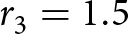 ${r_3} = 1.5$ mm. Considering these results, the optimal geometrical parameters were determined to be
 ${r_1} = 5$ mm and
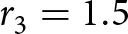 ${r_3} = 1.5$ mm to satisfy the reflection requirement at 6.2 GHz. The finalized structural dimensions are summarized in Table 2. Based on the optimized design, the FSS unit was subsequently integrated into the overall antenna configuration to verify its reflection and transmission performance.
Transmission coefficient of FSS unit. (a) Frequency selection unit. (b) Circuit structure corresponding to frequency selection unit. (c) Under different r1-value conditions. (d) Under different r3-value conditions.

Figure 8 Long description
The image A showing a circular ring shape with a central circular opening and a horizontal bar across the middle. Dimension arrows label w, r1, r2 and r3. The image B showing a rectangular circuit diagram with three horizontal branches. The top branch has an inductor symbol labeled L. The middle branch has a capacitor symbol labeled C. The bottom branch has an inductor symbol labeled L. The image C showing a line graph labeled (c). The x-axis is labeled Frequency(GHz), ranging from 4.5 to 7.5 with ticks at 4.5, 5.0, 5.5, 6.0, 6.5, 7.0 and 7.5. The y-axis is labeled S21(dB), ranging from 0 to minus 80 with ticks at 0, minus 10, minus 20, minus 30, minus 40, minus 50, minus 60, minus 70 and minus 80. A legend lists five curves: r1 equals 4.8mm, r1 equals 4.9mm, r1 equals 5.0mm, r1 equals 5.1mm and r1 equals 5.2mm. Each curve forms a single deep notch between about 6.0 and 6.6 on the frequency axis, returning toward 0 at lower and higher frequencies. The r1 equals 5.0mm curve reaches the lowest point, near minus 70 on the y-axis, at about 6.2 on the frequency axis. The other curves have minima that are higher (less negative) and occur slightly to the left or right of 6.2. The image D showing a line graph labeled (d). The x-axis is labeled Frequency(GHz), ranging from 4.5 to 7.0 with ticks at 4.5, 5.0, 5.5, 6.0, 6.5 and 7.0. The y-axis is labeled S21(dB), ranging from 0 to minus 80 with ticks at 0, minus 10, minus 20, minus 30, minus 40, minus 50, minus 60, minus 70 and minus 80. A legend lists five curves: r3 equals 1.3mm, r3 equals 1.4mm, r3 equals 1.5mm, r3 equals 1.6mm and r3 equals 1.7mm. Each curve forms a single deep notch between about 6.0 and 6.6 on the frequency axis, returning toward 0 at lower and higher frequencies. The r3 equals 1.5mm curve has a minimum near 6.15 on the frequency axis at roughly minus 55 to minus 60 on the y-axis. The other curves show minima at nearby frequencies with different depths.
Structural parameters of the FSS unit cell

Table 2 Long description
The table lists four structural parameters for an FSS unit cell and gives their values in millimeters. The parameters are r1, r2, r3, and w. r2 has the highest value at 6 mm, with r1 next at 5 mm. w is 4.2 mm, slightly smaller than r1. r3 is the smallest parameter at 1.5 mm. These values provide the relative sizing of the parameters but do not indicate tolerances, measurement uncertainty, or how each parameter is defined geometrically.
Feed structure design
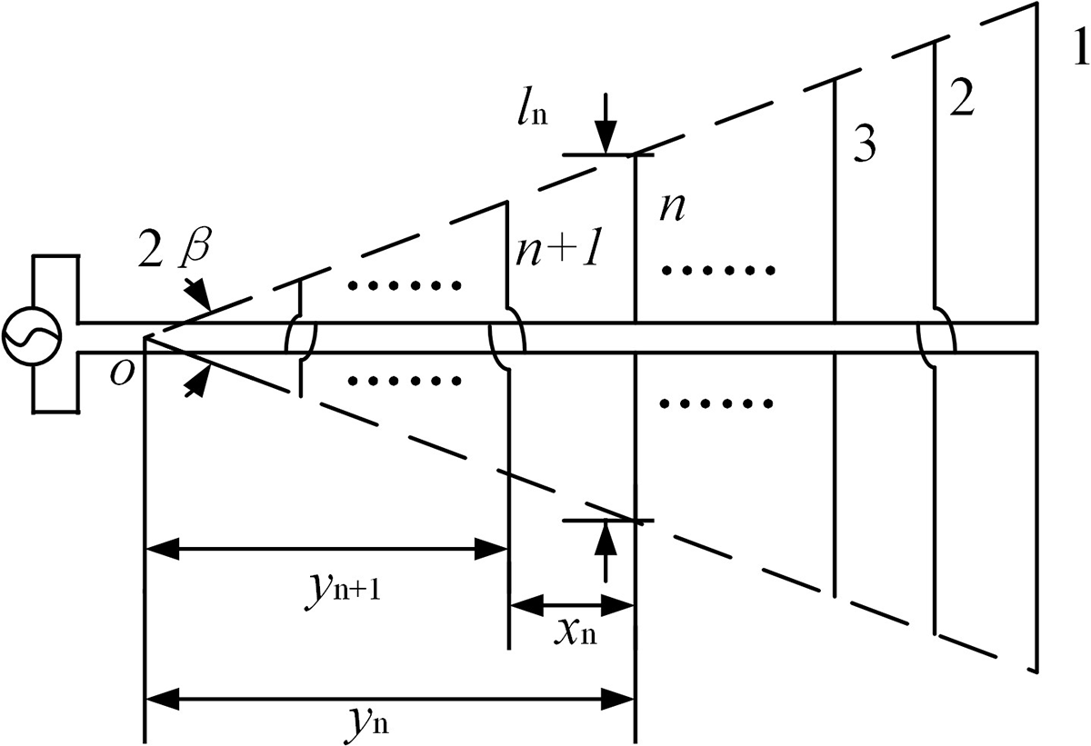
The log-periodic antenna structure consisting of multiple dipole elements arranged on a dielectric substrate is shown in Fig. 9. Designating the farthest element from the vertex as Index 1, the length of the nth symmetric dipole Ln, the spacing to its adjacent dipole xn, and the vertical distance from the vertex yn satisfy the following scaling relations:
Logarithmic cycle antenna.

Figure 9 Long description
The diagram illustrates a log-periodic antenna structure with multiple dipole elements arranged on a dielectric substrate. The farthest element from the vertex is labeled as Index 1. The elements are symmetrically arranged along a central axis, with each dipole labeled sequentially from n plus one to n and so on. The length of each dipole is denoted as l subscript n and the spacing to its adjacent dipole is x subscript n. The vertical distance from the vertex is labeled as y subscript n. The diagram includes dashed lines indicating the scaling relations between these elements, with arrows showing the dimensions l subscript n, x subscript n and y subscript n. The angle 2 beta is marked near the vertex, indicating the angular spread of the elements. The diagram visually represents the scaling relations that the lengths, spacings and vertical distances satisfy, as described in the context.
 \begin{equation}\tau = \frac{{{l_{n{\text{ + 1}}}}}}{{{l_n}}} = \frac{{{x_{n{\text{ + 1}}}}}}{{{x_n}}} = \frac{{{y_{n{\text{ + 1}}}}}}{{{y_n}}}\end{equation}
The geometric scaling factor τ, typically ranging from 0.8 to 0.95, defines the periodicity of the log-periodic antenna, governing the progressive scaling of dipole lengths and spacings to achieve frequency-independent radiation characteristics. In the above equation, the scaling factor is denoted as τ. As shown in Fig. 9, the included angle of the log-periodic antenna is 2α. For the nth symmetric dipole element, the following relationships can be derived:
 \begin{equation}\cot \beta = \frac{{{y_n}}}{{{l_n}/2}}\end{equation}
 \begin{equation}{x_n} = {y_n} - {y_{n{\text{ + 1}}}} = {y_n}(1 - \tau ) = \cot \beta \frac{{{l_n}}}{2}(1 - \tau )\end{equation}
The proposed design employs an LPDA fabricated on an FR4 dielectric substrate with a thickness of 0.8 mm, as illustrated in Fig. 10. The antenna consists of 15 symmetrically arranged dipole elements. The longest dipole element has a length of L 1 = 33.08 mm and a width of W 1 = 2.99 mm. The antenna is fed through a parallel twin-lead transmission line with a conductor width of 1.338 mm, terminated with a matched impedance load. A cross-fed configuration is adopted, with the feed point centrally located at the shortest dipole element. Adjacent dipoles are interconnected via parallel twin-lead transmission lines to establish a 180° phase reversal, thereby ensuring that the radiation is directed from the longest toward the shortest dipole element.
The structure of the Logarithmic cycle antenna as a feed.

Figure 10 Long description
The image shows a log-periodic dipole antenna design with two symmetrical sections. Each section contains multiple dipole elements arranged in a triangular pattern. The dipole elements are connected horizontally across the triangular structure, decreasing in size from top to bottom. The design is intended to facilitate efficient radiation from the longest to the shortest dipole element.
Figure 11 presents the simulated reflection coefficient of the feed antenna, indicating that within the frequency range of 4–7 GHz, the reflection coefficient remains below −20 dB, which confirms excellent impedance matching across the operating band.
The reflection coefficient of the logarithmic cycle antenna.

Figure 11 Long description
The y-axis label is “S1,1(dB)”. The y-axis ranges from minus 40 to minus 20, with labeled ticks at minus 20, minus 25, minus 30, minus 35 and minus 40. The x-axis label is “Frequency(GHz)”. The x-axis ranges from 4.0 to 7.0, with labeled ticks at 4.0, 4.5, 5.0, 5.5, 6.0, 6.5 and 7.0. A legend in the lower-right reads “Simulated” for a single line. The plotted line starts near 4.0 gigahertz at about minus 30 decibel, rises to around minus 25 decibel near about 4.3 gigahertz, then drops to a deep minimum near about 4.6 gigahertz at about minus 39 decibel. It rises again to around minus 25 decibel near about 5.0 gigahertz, then dips to around minus 28 decibel near about 5.3 gigahertz and rises to around minus 26 decibel near about 5.5 gigahertz. The line then drops to another deep minimum near about 6.0 gigahertz at about minus 40 decibel. After 6.0 gigahertz, the line rises to a broad high region near about 6.4 to 6.6 gigahertz at about minus 22 to minus 23 decibel, then falls toward 7.0 gigahertz to around minus 31 decibel.
The radiation patterns at 4.5, 5.5, and 6.5 GHz are shown in Fig. 12, demonstrating that the beam characteristics remain largely consistent over these frequencies. Specifically, the E-plane 3-dB beamwidths are 64.7°, 96.4°, and 104.6°, while the H-plane 3-dB beamwidths are 93.1°, 96.4°, and 104.6°, respectively. In addition, the corresponding antenna gains are 8.48, 8.32, and 8.00 dBi, confirming stable radiation performance within the operating band.
The radiation pattern of the logarithmic cycle antenna. (a) 4.5 GHz. (b) 5.5 GHz. (c) 6.5 GHz.

Figure 12 Long description
The radiation pattern of the logarithmic cycle antenna. (a) 4.5 GHz. (b) 5.5 GHz. (c) 6.5 GHz. The image A showing a polar line plot with two overlaid curves and a legend listing E-plane and H-plane. Angular tick labels around the circle are 0, 30, 60, 90, 120, 150, 180, 210, 240, 270, 300 and 330. The radial scale is labeled in decibel with tick labels 0, minus 10, minus 20, minus 30 and minus 40. Both curves form a main lobe centered at 0 degrees and a smaller lobe near 180 degrees. The image B showing a polar line plot with two overlaid curves and a legend listing E-plane and H-plane. Angular tick labels around the circle are 0, 30, 60, 90, 120, 150, 180, 210, 240, 270, 300 and 330. The radial scale is labeled in decibel with tick labels 0, minus 10, minus 20, minus 30 and minus 40. Both curves form a main lobe centered at 0 degrees and a smaller lobe near 180 degrees. The image C showing a polar line plot with two overlaid curves and a legend listing E-plane and H-plane. Angular tick labels around the circle are 0, 30, 60, 90, 120, 150, 180, 210, 240, 270, 300 and 330. The radial scale is labeled in decibel with tick labels 0, minus 10, minus 20, minus 30 and minus 40. Both curves form a main lobe centered at 0 degrees and a smaller lobe near 180 degrees.
Design of RA
As depicted in Fig. 13, the triple-band dual-layer microstrip reflection array antenna features a 200 mm × 200 mm aperture. The upper layer consists of an 11 × 11 main reflective surface array and an integrated 11 × 11 FSS. The lower layer incorporates an 11 × 11 array of cross-shaped reflection elements, which include integrated delay lines for phase control, along with a 10 × 10 array of Koch fractal cyclic radiation elements. This design leverages the optimized reflection unit and logarithmic periodic feed discussed previously.
The configuration of the reflectarray antenna. (a) Array stereogram. (b) Array side view.

Figure 13 Long description
The image A showing the array stereogram of a reflectarray antenna. It features a dual-layer structure with a 200 millimeter by 200 millimeter aperture. The upper layer consists of an eleven by eleven main reflective surface array, integrated with an eleven by eleven Frequency Selective Surface. The lower layer includes an eleven by eleven array of cross-shaped reflection elements, which incorporate integrated delay lines for phase control and a ten by ten array of Koch fractal cyclic radiation elements. The image B showing the side view of the array. It illustrates the height labeled as H and the width labeled as D. The side view provides a perspective on the arrangement of the elements along the surface, highlighting the vertical stacking and spacing of the components.
To achieve precise steering of the main beam, the compensation phase Φ i for each array element must be calculated. The corresponding phase compensation can be expressed as
 \begin{equation}{\phi _i} = 2\pi N + k\left( {{R_i} - {\operatorname{r} _i} \cdot {\operatorname{r} _o}} \right)\left( {N = 0,1,2\ldots} \right)\end{equation}
The corresponding phase compensation model for the RA involves the several parameters: k denotes the free-space wavenumber (k = 2π/λ 0), where λ 0 is the free-space wavelength at the central operating frequency; i represents the index of the ith radiating element within an array of N elements; Ri is the distance from the phase center of the feed antenna to the ith patch element; ri is the position vector from the center of the planar reflectarray to the center of the ith reflective element; and r 0 defines the steering vector along the main beam direction. For the center-feed configuration with the main beam aligned along the positive z-axis, the compensation phase Φi can be simplified as
 \begin{equation}{\phi _i} = 2\pi N + k{R_i}\end{equation}
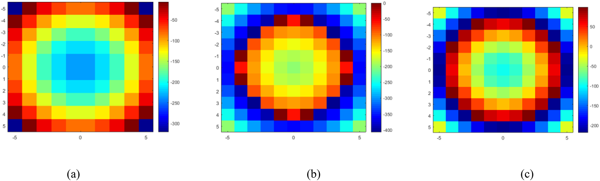
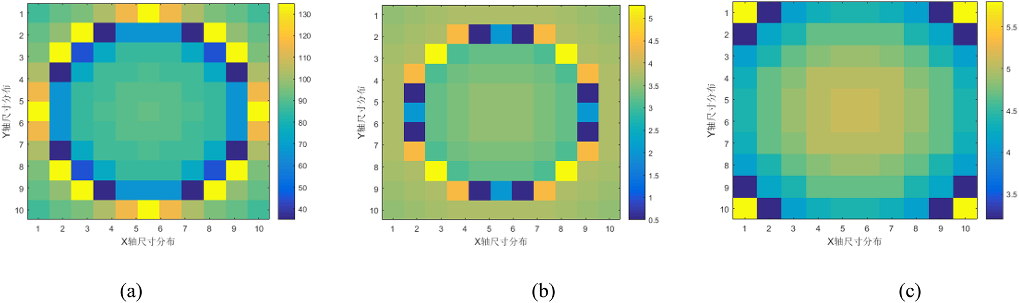
Empirical formulas were utilized to determine the feed height and compensation phase of each unit, resulting in the phase distribution diagram presented in Fig. 14. Additionally, optimization of unit dimensions yielded the corresponding unit size distribution, as shown in Fig. 15.
Phase distribution diagram. (a) Upper ring. (b) Koch fractal. (c) Cross unit.

Figure 14 Long description
The phase distribution diagram consists of three heatmaps labeled (a), (b) and (c). Image (a) is titled Upper Ring, showing phase distribution with axes ranging from negative 5 to 5. The color scale on the right indicates phase values, with darker shades representing higher phase values. Image (b) is titled Koch fractal, displaying phase distribution with similar axes and color scale, highlighting a central peak pattern. Image (c) is titled Cross unit, showing phase distribution with axes from negative 5 to 5 and a color scale indicating phase values, with elevated values in the center. The gradient runs from lighter to darker shades, denoting low to high phase values. The diagrams illustrate distinct phase patterns across the three units, emphasizing central peaks and variations in phase intensity.
Unit size distribution diagram. (a) Upper ring. (b) Koch fractal. (c) Cross unit.

Figure 15 Long description
The heatmaps illustrate unit size distribution across three geometries: Upper Ring, Koch fractal and Cross unit. Each heatmap has horizontal and vertical axes labeled 'X (mm)' and 'Y (mm)' respectively, with tick labels ranging from 1 to 10. The legends on the right of each heatmap indicate measurement intensity, with varying scales. Image A, labeled 'Upper Ring', shows a ring-shaped pattern with alternating blocks around the perimeter, indicating varying intensity levels. The central area is more uniform, suggesting lower intensity. Image B, labeled 'Koch fractal', displays a similar ring pattern with darker blocks interspersed, indicating higher intensity at specific points. The central area remains uniform, suggesting lower intensity. Image C, labeled 'Cross unit', features a broad central region with gradual changes toward the edges, forming a border-like pattern. The corners and outer edges show different intensity levels compared to the center. The legends indicate that higher values correspond to greater intensity, with Image A ranging from 0 to 200 and Images B and C ranging from 0 to 4.5. These heatmaps provide insights into the distribution and intensity of unit sizes across different geometrical configurations.
Design of RA
Figure 16 shows a photograph of the test environment for the multi-frequency reflectarray. To enhance the stability of the array, Substrate-2 is secured to Substrate-1 using insulating screws. The assembly of Substrate-1 and Substrate-2 is then connected together via a bracket, the top of which is attached to the feed source. In this section, the proposed array prototype is simulated and analyzed using CST Microwave Studio, and the reflection coefficient of the simulated RA at the operating frequencies is presented in Fig. 17. As shown in the figure, the reflection coefficient remains below −10 dB over the frequency range of 4.76–6.70 GHz, indicating good impedance matching across the operating band.
The fabricated reflectarray antenna and the measurement setup.

Figure 16 Long description
The image shows a test environment featuring a reflectarray antenna and a horn. The background consists of blue, pyramid-shaped acoustic panels. The reflectarray antenna is highlighted with red arrows pointing to its location. The horn is positioned to the right, also marked with a red arrow. Two insets display close-up views of the reflectarray antenna, showing its detailed pattern. The setup includes various equipment and structures, such as a stand and mounting brackets, used to support the components.
The measured and simulated |S 11| of the reflection array.

Figure 17 Long description
Vertical bar S subscript 1 1 vertical bar (decibel) A line graph with two curves and a legend in the upper right: Simulated and Measured. The horizontal axis is labeled Frequency (gigahertz), ranging from 4.2 to 6.6 with tick marks every 0.2. The vertical axis is labeled vertical bar S subscript 1 1 vertical bar (decibel), ranging from 0 at the top down to minus 45 at the bottom, with tick marks every 5. Simulated curve: Starts near minus 5 at 4.2 gigahertz, then shows many narrow dips between about 4.6 and 6.6 gigahertz. A deep dip reaches about minus 33 near 5.2 gigahertz. Another deep dip reaches about minus 33 near 6.4 gigahertz. Between dips, the curve is often between about minus 8 and minus 15. Measured curve: Starts near minus 5 at 4.2 gigahertz, then drops to about minus 45 near 4.35 gigahertz. From about 4.5 to 5.2 gigahertz it stays mostly between about minus 5 and minus 10. It then shows broader dips around the mid band, reaching about minus 15 to minus 18 near about 5.6 to 5.8 gigahertz. From about 6.0 to 6.6 gigahertz it stays mostly between about minus 10 and minus 15 with smaller dips.
The measured results indicate a noticeable frequency shift toward the lower end of the spectrum compared to the simulation. This discrepancy, along with a more pronounced performance degradation in the higher frequency band, is primarily attributed to manufacturing tolerances. These tolerances introduced slight substrate bending, which disturbed the critical impedance transformation relationship between the feed point and the fractal radiating elements. Furthermore, during measurement, the radiation from the RF cable in close proximity to the coaxial probe likely interacted with the antenna, further compromising the results.
Figure 18(a)–(c) presents the simulated E-plane radiation patterns of the proposed RA at 4.8, 5.2, and 6.2 GHz, respectively. The main beam direction remains stable across these frequencies, with sidelobe levels suppressed below −17.1, −18.3, and −15 dB, while the cross-polarization levels are consistently maintained below −30 dB at these frequencies.
The E-plane patterns of the antenna and the H-plane patterns of the antenna at working frequencies. (a) 4.8 GHz. (b) 5.2 GHz. (c) 6.2 GHz.

Figure 18 Long description
The image shows six polar plots of antenna radiation patterns at three frequencies: 4.8 GHz, 5.2 GHz and 6.2 GHz. Each plot displays E-plane and H-plane patterns with co-polar and cross-polar responses. The radial axis represents gain in decibels, ranging from 0 to minus 30 decibels. The angular axis is labeled in degrees from 0 to 360. In the first column (a), the frequency is 4.8 GHz. The E-plane plot shows a main lobe centered at 0 degrees with sidelobe levels below minus 17.1 decibels. The H-plane plot also has a main lobe at 0 degrees, with sidelobe levels below minus 17.1 decibels. In the second column (b), the frequency is 5.2 GHz. The E-plane plot maintains a stable main lobe at 0 degrees, with sidelobe levels below minus 18.3 decibels. The H-plane plot shows similar characteristics, with sidelobe levels below minus 18.3 decibels. In the third column (c), the frequency is 6.2 GHz. The E-plane plot has a main lobe at 0 degrees, with sidelobe levels below minus 15 decibels. The H-plane plot mirrors this pattern, with sidelobe levels below minus 15 decibels. Each plot includes simulated and measured data, distinguished by line styles and labels in the legend. Co-polar responses are dominant, while cross-polar responses remain low across all frequencies. The main beam direction remains stable and cross-polarization levels are consistently below minus 30 decibels.
Similarly, the H-plane radiation patterns, also shown in Fig. 18(a)–(c), exhibit sidelobe levels of −12.6, −14.9, and −14.3 dB at 4.8, 5.2, and 6.2 GHz, respectively. The cross-polarization levels remain below −30 dB at 4.8 and 6.2 GHz, and below −29 dB at 5.2 GHz, demonstrating good polarization purity across the operating band.
Figure 19 shows the directional map simulations of the reflect array antenna in the E-plane and H-plane at other frequencies. In the E-plane, the simulated sidelobes are on average less than −13 dB at 4.5, 5.5, 6.0, and 6.4 GHz. For the cross-polarization level of the antenna, it is less than −32 dB at these frequencies. In the H-plane, the simulated sidelobes are on average less than −10 dB, and the cross-polarization level of the antenna is on average less than −22 dB.
The E-plane patterns of the antenna and the H-plane patterns of the antenna at other frequencies. (a) Main polarization. (b) Cross-polarization.

Figure 19 Long description
The image consists of four line graphs depicting antenna radiation patterns. Each graph compares the E-plane and H-plane patterns at frequencies of 4.5 GHz, 5.0 GHz, 5.5 GHz, 6.0 GHz and 6.4 GHz. Graph (a) shows the main polarization in the E-plane with solid lines. The x-axis is labeled angle in degrees, ranging from -180 to 180 degrees. The y-axis is labeled radiation magnitude in decibels, ranging from -40 to 20 decibels. Peaks are observed around 0 degrees, with sidelobes less than -13 decibels. Graph (b) shows the cross-polarization in the E-plane with dashed lines. The x-axis and y-axis are similarly labeled. Sidelobes are less than -32 decibels, with a more dispersed pattern. Graph (c) shows the main polarization in the H-plane with solid lines. The x-axis is labeled angle in degrees, ranging from -180 to 180 degrees. The y-axis is labeled radiation magnitude in decibels, ranging from -40 to 20 decibels. Peaks are observed around 0 degrees, with sidelobes less than -10 decibels. Graph (d) shows the cross-polarization in the H-plane with dashed lines. The x-axis and y-axis are similarly labeled. Sidelobes are less than -22 decibels, with a more dispersed pattern. Across all graphs, the main lobe direction is consistently around 0 degrees, with varying sidelobe levels and patterns across different frequencies.
The simulated radiation gain performance of the reflect array antenna is depicted in Fig. 20, which demonstrates a peak gain of 19.9 dBi at 6.2 GHz, with additional gains of 17.1 dBi at 4.8 GHz and 18.7 dBi at 5.2 GHz. Furthermore, the simulated gain exceeds 16 dBi across frequencies spanning from 4.46 to 6.43 GHz, demonstrating stable performance over a 1.97 GHz operational bandwidth.
Simulated and measured gain of the proposed antenna.

Figure 20 Long description
The x- axis represents Frequency(GHz) from 4.4 to 6.6 in increments of 0.2. The y- axis represents Gain(dBi) from 8 to 22 in increments of 2. A legend lists Simulated and Measured. Simulated series points: (4.4, 14), (4.5, 17), (4.6, 16.8), (4.7, 16.6), (4.8, 17.2), (4.9, 17.0), (5.0, 18.0), (5.1, 17.2), (5.2, 18.2), (5.3, 18.4), (5.4, 17.0), (5.5, 16.0), (5.6, 17.6), (5.7, 17.4), (5.8, 18.6), (5.9, 18.2), (6.0, 18.2), (6.1, 18.0), (6.2, 19.0), (6.3, 19.0), (6.4, 17.5), (6.5, 13.5), (6.6, 11.0). Measured series points: (4.4, 13.0), (4.5, 16.8), (4.6, 16.4), (4.7, 16.2), (4.8, 16.6), (4.9, 16.6), (5.0, 17.6), (5.1, 16.8), (5.2, 18.0), (5.3, 18.2), (5.4, 16.8), (5.5, 16.2), (5.6, 17.2), (5.7, 17.2), (5.8, 18.2), (5.9, 18.0), (6.0, 18.0), (6.1, 18.0), (6.2, 18.2), (6.3, 18.2), (6.4, 16.8), (6.5, 11.2), (6.6, 10.0). Across 4.4 to 6.3, both series stay mostly between 16.0 and 19.0. The simulated series reaches 19.0 at 6.2 and 6.3 and the measured series reaches 18.2 at 6.2 and 6.3. Both series drop from 6.4 to 6.6, with simulated changing from 17.5 at 6.4 to 11.0 at 6.6 and measured changing from 16.8 at 6.4 to 10.0 at 6.6. The lowest listed values occur at 6.6 for both series.
Table 3 compares the proposed reflectarray with several representative designs. The proposed antenna employs a subwavelength triple-resonant unit cell, enabling a wide phase tuning range of 360°, which is larger than that reported by Luyen et al. [Reference Luyen, Zhang, Booske and Behdad10]. Meanwhile, the antenna maintains a compact aperture size of 200 × 200 mm2, smaller than that reported by Wu et al. [Reference Wu, Hu, Luo, Zhao, Jiang and Chen7]. Despite the reduced aperture, the proposed design achieves peak gains of 17.1–19.9 dBi with a low cross-polarization level of −29.82 dB and a sidelobe level of −12.13 dB. These results indicate that the proposed reflectarray provides a favorable tradeoff among aperture size, phase control capability, and radiation performance.
Performance comparison of the proposed antenna with related works

Table 3 Long description
The table compares four antenna designs across operating frequency, design approach, aperture size, element count, phase shift range, peak gain, sidelobe level, and cross polarization. This work operates at 4.8, 5.2, and 6.2 GHz using a subwavelength triple resonance mechanism, with a 200 by 200 millimeter aperture and element counts of 100, 121, and 121 across the three bands. Its phase shift range is 360, 340, and 355 degrees, and peak gain rises from 17.1 to 18.7 to 19.9 dBi across the three frequencies. Reference 7 uses a 3D resonant element at 15 GHz with a larger 240 by 240 millimeter aperture and 900 elements, achieving 24.5 dBi peak gain but a smaller 315 degree phase range and no reported sidelobe or cross polarization values. Reference 10 uses a reconfigurable polarization rotating phase shifter at 10 GHz with a 192 by 192 millimeter aperture and 256 elements, reaching 18.5 dBi peak gain with a 180 degree phase range and no reported sidelobe or cross polarization values. Reference 11 is a single layer multi resonant design at 37 GHz with an 80 by 80 millimeter aperture and 400 elements, reporting 27.86 dBi peak gain, sidelobe level below minus 17.93 dB, and cross polarization below minus 25 dB, but no phase range. Comparisons are limited because several entries omit sidelobe level, cross polarization, or phase shift range.
Conclusion
A novel C-band wideband RA utilizing double-layered sub-wavelength elements has been presented. This antenna features an upper-layer structure comprising a frequency-selective unit with a circular ring internally connected to two open-circuited stubs and a reflecting element loaded with double-arc delay lines, while the lower dielectric substrate integrates first-order Koch fractal-inspired Phoenix loop units and cross-shaped patch-loaded delay lines as reflecting elements; driven by an ultra-wideband log-periodic feed (centrally fed via SMA connector at the shorter dipole, radiating from the longer to the shorter dipole) for a 200 mm × 200 mm reflectarray aperture with the phase center positioned 83.7 mm above its center, it achieves a simulated −10 dB impedance bandwidth spanning 4.76–6.70 GHz, exhibits measured E-plane sidelobe levels below −12.13 dB and cross-polarization under −29.82 dB at 4.8, 5.2, 6.2 GHz, demonstrates H-plane sidelobes under −11.05 dB and cross-polarization below −27.27 dB at identical frequencies, and delivers a peak gain of 19.9 dBi at 6.2 GHz.
Funding statement
This work was supported by the National Science Foundation of China (62071282).
Competing interests
The authors report no conflict of interest.

Yunlong Wu received the B.E. degree in electronic information engineering from Taiyuan Institute of Technology, Taiyuan, China, in 2022. He is currently pursuing the M.S. degree with the School of Physics and Electronic Engineering, Shanxi University, Taiyuan, China. His current research interests include reflectarray antennas, wideband antennas, electrically small antennas, and metasurface-based antenna design.

Zhiyuan Yang received the B.E. degree in communication engineering from Hebei University, Baoding, China, in 2020, and the M.S. degree in communication engineering from Shanxi University, Taiyuan, China, in 2023. His research interests include antenna design, reflectarray antennas, and microwave and wireless technologies.

Yufeng Liu was born in Shanxi Lvliang, China, in 1986. He received the PhD degree in radio physics from Sichuan University, Sichuan, China,in 2014. In 2015, he joined the College of Physics and Electronic Engineering, Shanxi University. His research is mainly focused on computational electromagnetics and antenna design.