The American labor market was at a crossroads of major transitions and economic events in the middle of the twentieth century. With the first generation of workers educated in America’s rapidly expanding high school system entering the labor force, the “human capital century” was well underway (Goldin and Katz Reference Goldin and Katz2009). While the aftershocks of the Great Depression were still reverberating in 1940, the economic and social upheaval of World War II (WWII) had yet to hit the country. The Great Compression—a period of declining wage dispersion that saw earnings inequality shrink across education, experience, and occupation groups—was also just beginning (Goldin and Margo Reference Goldin and Margo1992).
The relative price paid for educated or skilled workers—an important feature of any economy—is vital to the scholarly understanding of the American economy at mid-century as the supply of skilled workers rose and inequality fell. In recent decades, growth in the skill premium explains about two-thirds of the rise in inequality (Goldin and Katz Reference Goldin and Katz2007) and income inequality is much higher at the end of the twentieth century than it was at mid-century (Saez Reference Saez, David and Hill2018; Kopczuk, Saez, and Song Reference Kopczuk, Saez and Song2010). If slowing growth in the supply of educated workers (Goldin and Katz Reference Goldin and Katz2009) drives inequality today, did expansion in the supply at mid-century have the opposite effect? If mass education helped tamp down inequality, lower returns to schooling would be clear evidence. Correlations between education and earnings point in this direction: Goldin and Katz (Reference Goldin and Katz2009) trace out a U-shaped pattern in the skill premium that reaches its nadir at mid-century. The high school premium was lower in 1940 than it had been in 1915, while the college premium was lower in 1940 than it is today.Footnote 1
However, the trends documented by Goldin and Katz (Reference Goldin and Katz2009) are based on associations rather than causal estimates—the claim that education returns were lower at mid-century thus needs to be re-investigated. Self-selection may bias simple Mincerian correlations. If high-ability individuals tend to acquire more years of schooling, then any positive association between earnings and education might reflect the higher productivity of such people, independent of schooling. That is, the skill premium could be biased upwards. On the other hand, if the opportunity cost of education pushes high-potential earners out of school earlier, then the estimates would be biased downwards. While studies suggest that the bias in Mincerian regressions is small in the late twentieth century (Card Reference Card, Ashenfelter and Card1999), this may or may not have been true further back in time. Beyond selection bias, measurement error in years of schooling might also vary over time, and such error could attenuate the estimated returns. With different forces at play, the overall direction of bias in the Mincerian correlations is unclear, especially during a period of large changes in the labor market. We offer a new look at the return to schooling in the middle of the twentieth century, paying particular attention to both selection and measurement error.
To identify the causal effect of education on earnings, we construct a large linked sample of twin brothers who grew up in the same families and compare their education and earnings during adulthood. If twins have similar innate characteristics or abilities, a within-twins comparison can then be used to address the confounding effects of unobserved differences.
Applying the within-twins estimator to a historical setting offers two key advantages. First, the same approach has been used to estimate the return to schooling for more recent cohorts. To the extent that any inherent biases in the twins method are similar in the past and present, this allows us to compare our estimates with twins studies in the late twentieth century and to shed light on how the value of education has changed over more than 50 years. Second, the availability of the complete historical census records enables us to construct samples of twins that are both larger in size and wider in geographic coverage than other twins studies, many of which rely on small samples from local surveys or state-specific registers.
We undertake our analysis recognizing the limitations of the twins methodology. Some of these weaknesses are common across twins studies, while others are specific to our historical setting and data. A major critique of all twins studies is that even identical twins are not exactly the same. The research design only “works” if twin brothers complete different years of education, but such differences could arise from unobserved differences in characteristics that might compromise the identifying assumption of the within-twins estimator. Both the size of our twins sample and the availability of names in the historical censuses allow us to introduce new tests to assess the extent of ability bias in our estimates, tests that are not always feasible with contemporary data. While we cannot completely rule out ability differences between twins and our new tests rely on assumptions about parent behavior, the evidence as a whole suggests that our baseline findings are unlikely to be driven by such confounders.
Studying twins in a historical setting presents its own unique challenges, many of which we are able to address. First, we need to link individuals across censuses to identify twins and construct our key variables. Without unique individual identifiers, the historical census linking process is never perfectly accurate. Reassuringly, our results are robust to alternative linking methods.Footnote 2 Second, we can only link men—a common constraint in the census linking literature—and are thus able to estimate the return to education from male-male twin pairs only. Third, contemporary twins studies often exploit a twin’s report of his or her sibling’s education to address measurement error in self-reported schooling. As such information is not available in the censuses, we use key milestones in education attainment—which respondents may be more likely to remember—to provide alternative evidence that measurement error in education is unlikely to be driving our results. Fourth, it is not possible to distinguish monozygotic (MZ) and dizygotic (DZ) twins in the historical data. MZ twins are the preferred study population, as they share both the same genes and the same environment. However, even same-sex twins can be wrong about their identical-versus-fraternal status; for example, nearly one-fifth of twins were wrong in the Add Health longitudinal study (Conley and Fletcher Reference Conley and Fletcher2017, Chapter 2). Consequently, MZ and DZ status may not be well-measured in recent studies either. Moving beyond genetic similarity, we introduce measures of twin name similarity that may capture how similarly parents intend to treat their twins. This provides a proxy for “identicalness” in nurture rather than nature.Footnote 3
We find that the return to education in the United States was positive in 1940 but smaller than the estimates for more recent periods. The positive historical returns arise from education affecting both access to “better” jobs as well as earnings within occupations, with the latter driving two-thirds of the effect. Returns in the late twentieth century tend to be relatively large across different identification strategies (Card Reference Card, Ashenfelter and Card1999), including within-twins comparisons (Ashenfelter and Krueger Reference Ashenfelter and Krueger1994; Ashenfelter and Rouse Reference Ashenfelter and Rouse1998; Rouse Reference Rouse1999; Behrman and Rosenzweig Reference Behrman and Rosenzweig1999), the quarter-of-birth instrument (Angrist and Keueger Reference Angrist and Keueger1991), and the distance-to-college instrument (Card Reference Card1993). Our smaller historical results, juxtaposed with the larger returns more recently, are consistent with the U-shaped trend in Goldin and Katz (Reference Goldin and Katz2009).Footnote 4
Our large sample of twins also enables us to estimate the return to education across two important background characteristics, shared by twins but differing across pairs. First, returns are higher for twin sons whose fathers were farmers or were of lower socio-economic status (SES). Second, the value of schooling varies by family immigration history: twin brothers with more foreign-born grandparents earn relatively less with years of education held constant, possibly due to differences in the quality of schools attended by the descendants of immigrants and the U.S.-born.
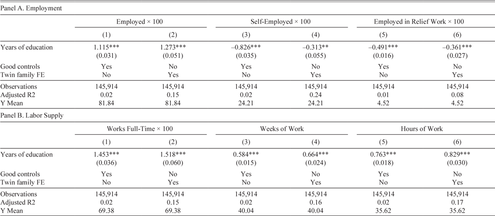
We also use the twins research design to study the effect of education on outcomes beyond earnings. We show that twins with more schooling had a higher probability of being employed and also supplied more weeks and hours of labor. Additional years of education lowered rates of self-employment and relief employment, as well. Finally, those who had more education were also more likely to migrate but less likely to have children, though the magnitudes of these effects are relatively small.
In estimating the return to education at mid-century, our article is closest to Clay, Lingwall, and Stephens (Reference Clay, Lingwall and Stephens2016), who exploit early twentieth-century changes in compulsory schooling laws (CSLs) to instrument actual education attainment with compelled years of schooling, differencing out cohort and state-of-birth fixed effects.Footnote 5 To estimate the CSL effects, Clay, Lingwall, and Stephens (Reference Clay, Lingwall and Stephens2016) compile a new dataset of CSLs across states from 1880 to 1930. They find returns of 6.4 to 7.9 percent using the 1940 census, which overlaps with the lower range of estimates for more recent cohorts. The CSL-based identification strategy also enables Clay, Lingwall, and Stephens (Reference Clay, Lingwall and Stephens2016) to estimate the returns throughout the earnings distribution with quantile regressions. In addition, while Clay, Lingwall, and Stephens (Reference Clay, Lingwall and Stephens2016) focus on white men, their CSL method can be applied to women and minority groups who are difficult to link accurately across censuses. However, unlike the twins approach, it is difficult to compare their historical results with contemporary studies. There are two reasons for this. First, Stephens and Yang (Reference Stephens and Yang2014) show that the return to schooling estimated in contemporary CSL studies can be eliminated by allowing birth year effects to vary by region. This null result deviates from most other recent estimates of the return to education. Second, intertemporal comparisons are challenging with the CSL approach because education levels have changed over time. When educational attainment in the population rises faster than the CSL thresholds—as it did in the United States over the twentieth century (Goldin and Katz Reference Goldin and Katz2009)—the CSL compliers or those on the margin of treatment change as well. Clay, Lingwall, and Stephens (Reference Clay, Lingwall and Stephens2016) show that the early CSLs primarily affected people in the later years of common school with around six, seven, or eight years of education. Compliers of more recent CSLs will instead be in high school. In contrast, because twinning is closer to random—at least prior to recent advances in fertility treatment (Kulkarni et al. Reference Kulkarni, Jamieson and Howard2013)—the study populations in the past and present may be more comparable. Treatment effects estimated from twins may also be closer to the population parameter as we observe people across the education distribution.
The article proceeds as follows. We begin by describing our historical sample of twins, including details on the complete count census data we draw on and the census-to-census linking method we use. We then present our estimated return to education in 1940 and provide several robustness tests. Beyond these average estimates, we also use our large sample of twins to explore whether there were any heterogeneous returns by family status and immigration history. This is followed by an analysis of how education may have affected other outcomes beyond earnings, such as labor supply, migration, and family structure.Footnote 6
HISTORICAL SAMPLE OF TWINS
Complete Count Census Data
Our main variables of interest, years of schooling and weekly earnings, come from the complete records of the 1940 Federal Census. These data are available through the Integrated Public Use Microdata Series (IPUMS) (Ruggles et al. Reference Ruggles, Flood, Goeken, Grover, Meyer, Pacas and Sobek2020). We estimate the return to education in 1940 and no other year for three reasons. First, education and earnings were not recorded in federal censuses before 1940.Footnote 7 Second, the complete census enumerations with names are essential for linking individuals, but these are only made available 72 years after a given census is taken to protect the privacy of respondents. The 1940 records are thus the latest available full counts. Third, the return to schooling in the middle of the twentieth century is inherently interesting: Mincerian estimates of education returns in 1940 are low, possibly due to the influx of educated workers coming out of the high school movement (Goldin Reference Goldin1998), even as demand for skilled workers was growing during the middle of the human capital century.
The 1940 census measures educational attainment as the “highest grade of school completed.” Enumerators were instructed to ask the education question of everyone and not to include half years or unfinished grades. The average male worker in 1940 had 8.6 years of schooling, with 24.8 percent finishing at least high school and 6.0 percent completing college.Footnote 8 In practice, years of education is top-coded at five or more years of college, but this affects just 1.5 percent of the population. Though commonly used in the economic history literature, the measure of education in the 1940 census has its limitations. For example, it does not adjust for school quality, which was considerably worse for African Americans at the time (Margo Reference Margo1986). Measuring educational attainment based on grade completion is also a distinct concept from years of schooling, particularly for African Americans who, on average, took more than a year to complete a grade and who often attended ungraded schools (Margo Reference Margo1986). However, as our baseline sample of twins primarily consists of whites, these quality issues with the education data are unlikely to be crucial to our conclusions.
Our main outcome of interest is the log of weekly earnings.Footnote 9 We construct weekly earnings by dividing annual labor earnings by the reported number of weeks worked. We note five important points about this measure. First, both annual earnings and weeks worked refer to the 1939 calendar year, asked when the census was conducted in April 1940. Second, unlike later censuses, the 1940 census only recorded wage and salary earnings. We are thus unable to study how education affected earnings from businesses or other sources and will need to restrict our analysis to wage and salary workers. Third, wage responses were top-coded at $5,000, although only 1 percent of our twins sample was top-coded. Fourth, with just one year of labor earnings, we have a noisy measure of permanent earnings, which may be the more relevant concept when estimating the return to schooling. Fifth, the number of weeks worked may also be measured with error.
Locating Twins in the Censuses
We identify twin brothers in the complete enumerations of the 1900, 1910, and 1920 censuses (Ruggles et al. Reference Ruggles, Flood, Goeken, Grover, Meyer, Pacas and Sobek2020). Twin brothers are defined as any pair of male siblings living in the same household who have the same last name, age in years, birthplace, and relationship to the household head. As with most analyses involving linked historical data, we focus on men because women tend to change their last names upon marriage during this period, making it difficult to track them across censuses. Our sample thus excludes any girl-girl or boy-girl twin pairs. By using the full counts, we are able to observe the universe of boy-boy twins in each base year. This compensates for the rarity of twin births and imperfections in record linkage, both of which shrink the final sample size.
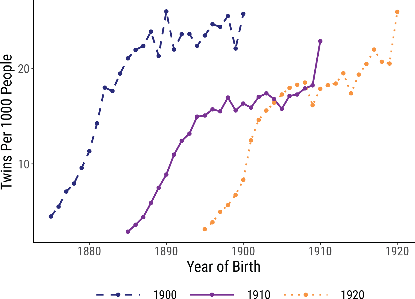
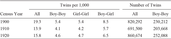
From the full counts, we identify approximately 900,000 children, aged 0 to 25, in each decennial census who have a twin sibling. Of these, more than 200,000 are in boy-boy pairs.Footnote 10 We plot the overall twin rate in Figure 1 and describe the rate and number of twins by census year in Table 1. As Figure 1 makes clear, we are more likely to identify twins among younger children or those born closer to the enumeration year. This reflects our procedure for identifying twins: children need to be residing in their childhood households with their same-age siblings before they can be tagged as twins, but older children are more likely to have left home, preventing us from finding older twins.
TWINS PER 1,000 PEOPLE IN THE COMPLETE COUNT CENSUSES, 1900–1920
Notes: We construct estimates of the number of twins in the United States in each decennial census from 1900 to 1920. We identify twins as two people aged 25 or younger living in the same household with the same last name, age in years, birthplace, and relationship to the household head. To calculate the number of twins per 1,000 people, we count the number of people aged 25 or younger as the denominator.
Source: Ruggles et al. (Reference Ruggles, Flood, Goeken, Grover, Meyer, Pacas and Sobek2020).

TWINS IN THE U.S. CENSUSES, 1900–1920

Notes: We construct estimates of the number of twins in the United States in each decennial census from 1900 to 1920. We identify twins as two people aged 25 or younger living in the same household with the same last name, age in years, birthplace, and relationship to the household head. To calculate the number of twins per 1,000 people, we count the number of people aged 25 or younger as the denominator.
Source: Ruggles et al. (Reference Ruggles, Flood, Goeken, Grover, Meyer, Pacas and Sobek2020).
Historically, is the frequency of twinning high or low? As we document in Table 1, we identify approximately 15 twins per 1,000 people. This is lower than the contemporary rate of 33.3 twins per 1,000 people (Martin et al. Reference Martin, Hamilton, Ventura, Osterman, Wilson and Mathews2012). There are three reasons for this. First, our sample includes everyone aged 25 or younger but we are unable to pick out twins if either twin has left the childhood household. Second, the advent of fertility treatments substantially raised the likelihood of twin births. Kulkarni et al. (Reference Kulkarni, Jamieson and Howard2013) estimated that by 2011, 36 percent of twin births in the United States were due to fertility treatments such as in-vitro fertilization. Third, child mortality rates in the United States are lower today than they were in the early twentieth century (Preston and Haines Reference Preston and Haines1991). Because our method of identifying twins requires both twins to reside in their childhood household when the decennial census is taken, children born as twins but whose twin sibling is deceased will not be identified as twins.
Record Linkage
We construct the linked sample of twins using the machine learning approach introduced by Feigenbaum (Reference Feigenbaum2016). This procedure begins by searching for the space of all potential matches based on name, birthplace, race, and implicit year of birth.Footnote 11 A random subsample is then drawn and manually matched or “trained” by a human researcher. Humans tend to be reasonably good at identifying links, even on messy data, but the rules they use to do so are opaque and difficult to write down. The machine learning method makes the implicit importance of various record features in determining a match explicit, capturing the weights on different features as covariates in a probit model. The resulting estimates are used to generate probabilistic scores for all potential matches. To be considered a true match, these scores need to be sufficiently high both in absolute terms and relative to any alternative options.Footnote 12 This produces a preliminary linked sample of 312,369 individuals with a match rate of 45 percent.Footnote 13 Later, we show that our results are robust to altering how conservative the machine learning procedure is, and to using the more classic approach to record linkage outlined by Abramitzky, Boustan, and Eriksson (Reference Abramitzky, Boustan and Eriksson2012).
Baseline Sample
We impose three restrictions on the preliminary linked sample. First, only twin pairs where both brothers can be linked to 1940 are kept, since the return to schooling will be identified from within-twins variation. Second, we limit the sample to twin pairs where both brothers are wage and salary workers in 1940.Footnote 14 As stated earlier, the 1940 census records earnings from wages but no other sources of income. Consequently, the earnings of self-employed people are likely understated.Footnote 15 Third, to ensure that our results are not driven by outliers, both brothers are required to have worked a positive number of weeks in the previous year, a positive number of hours in the preceding week, and to have earned at least $6 a week.Footnote 16 The final dataset comprises 38,652 individuals or 19,326 pairs of twins.Footnote 17
Our twins sample is large compared with datasets of twins from the late twentieth century that have been used to estimate the return to schooling. Ashenfelter and Krueger (Reference Ashenfelter and Krueger1994) and Ashenfelter and Rouse (Reference Ashenfelter and Rouse1998), for example, have 149 and 340 pairs of U.S. twins, respectively. Drawing on data from the United Kingdom, Bonjour et al. (Reference Bonjour, Cherkas, Haskel, Hawkes and Spector2003) study 214 pairs. Samples based on Scandinavian registry data tend to be larger. Bingley, Christensen, and Walker (Reference Bingley, Christensen and Walker2009), for instance, have information on 4,809 pairs of Danish twins, while Isacsson (Reference Isacsson2004) looks at 6,210 pairs of Swedish twins.
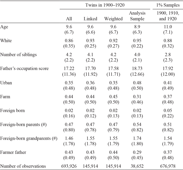
We compare our sample both as children and as adults to the general population and find that while our linked twins are more likely to be white and significantly less likely to be foreign born, they are not an extreme subset of the population.
We compare twins and their families in 1900, 1910, and 1920 to their cohort-mates in Table 2. To draw cohort-mates, we pull a 1 percent random sample from all boys aged 25 or younger who are not the head or head’s spouse in the 1900, 1910, and 1920 censuses.Footnote 18 We note three differences here. First, twins tend to be younger, possibly because the likelihood of identifying twins declines with age as individuals leave their childhood households. Second, linked twins are more likely to be white—95 percent of our analysis sample is white, compared with 86 percent in the full population of twins. This may be driven by the relative difficulty of linking non-white records across censuses. Third, and unsurprisingly, twins are likely to have more siblings than a random age-mate from the population. These three differences, coupled with other small differences in Table 2, suggest some caution when extrapolating the return to schooling for twins to the general population.
TWINS AND THEIR FAMILIES ARE SIMILAR TO THE AMERICAN POPULATION, 1900–1920

Notes: Means with standard deviations below in parentheses. In the first four columns, we summarize the twins identified in 1900, 1910, and 1920. Column 2 presents the linked twins, unweighted, while Column 3 uses inverse propensity weights to account for differences between census matched and unmatched twins. Column 4 limits the sample to our analysis sample, focusing only on the twins who were wage and salary male workers with a weekly wage of at least $6, who worked a positive number of weeks in the previous year (1939), and who worked a positive number of hours in the previous week. The twins sample includes only twins who both fit our sample criteria. Finally, Column 5 presents summary statistics for boys aged 25 or younger who were residing in their parents’ households in 1900, 1910, and 1920, based on three 1 percent random samples. Standard deviations are in parentheses.
Source: Ruggles et al. (Reference Ruggles, Flood, Goeken, Grover, Meyer, Pacas and Sobek2020).
We also find that twins are broadly similar to their cohort-mates during adulthood. Table 3 compares our twins with a 1 percent random sample drawn from the 1940 census. For consistency, the comparison group is restricted to male wage and salary workers aged 17 to 68, and the same sample restrictions in the baseline sample are imposed on wages, weeks worked, and hours worked. Linked twins are more likely to be married and less likely to be foreign born. The latter could reflect the fact that a substantial share of immigrants Americanize their names (Biavaschi, Giulietti, and Siddique Reference Biavaschi, Giulietti and Siddique2017), which lowers the odds of matching them across censuses by name.
LINKED TWINS ARE SIMILAR TO THE AMERICAN POPULATION IN 1940

Notes: In Columns (1) and (2) we summarize our linked sample of twin brothers, linking twins from the 1900, 1910, and 1920 censuses to 1940. Column (1) are the linked twins, unweighted, while Column (2) uses inverse propensity weights to account for differences between census matched and unmatched twins. We limit the twins to our analysis sample, focusing only on the twins who were wage and salary male workers with a weekly wage of at least $6, who worked a positive number of weeks in the previous year (1939), and who worked a positive number of hours in the previous week. The twins sample includes only twins who both fit our sample criteria. In Column (3), we use a random 1 percent sample of the 1940 census. For consistency, the 1940 1 percent sample is limited to employed men aged 17–68 who are wage and salary workers and we impose the same sample restrictions on wages, weeks worked, and hours worked. Standard deviations are in parentheses.
Source: Ruggles et al. (Reference Ruggles, Flood, Goeken, Grover, Meyer, Pacas and Sobek2020).
In the Online Appendix, we also show that the education and earnings distributions for our linked twins and the general population in 1940 overlap closely (Figure A.5 and Figure A.6).
THE RETURN TO SCHOOLING IN THE FIRST HALF OF THE TWENTIETH CENTURY
Empirical Strategy
The twins identification strategy has a long history in labor economics as a method of estimating the causal return to education. Naive comparisons of earnings and schooling may overstate the rate of return, as individuals with more schooling may also have higher unobserved ability.Footnote 19 An imperfect solution is to compare siblings within a household to reduce the bias from nurture-induced differences in ability. The within-twins comparison goes one step further. MZ twins have near-identical genetic makeups, allowing researchers to better “control” for nature and nurture.Footnote 20 DZ twins are no more genetically related than any pair of siblings but are of the same age—they will thus be subject to common cohort-specific time-varying shocks and share more similar family environments than siblings of different ages.
To determine how an additional year of schooling affects earnings, we implement the following regressions with our linked sample of twins:
 $$\log {W_{ih}} = \alpha + {\beta ^{OLS}} \cdot Sch{l_{ih}} + {X_{ih}} + {\varepsilon _{ih}}$$
 $$\log {W_{ih}} = \alpha + {\beta ^{FE}} \cdot Sch{l_{ih}} + {\gamma _h} + {X_{ih}} + {\varepsilon _{ih}}$$
for individual i and household h. The outcome is the log weekly wage, logW, and the main independent variable is the years of schooling, Schl, based on the highest grade completed. Regression (1) is a simple OLS benchmark that uses variation both across and between all twin brothers. Regression (2) implements the twins design by adding in family fixed effects, γ, exploiting only variation between twins to estimate the return to education.
We partition the set of controls, X, into two groups. The first is a vector of predetermined characteristics: a quadratic in age, a race dummy, and an indicator for foreign-born people. As these controls do not vary between twins, they are effectively dropped in our preferred specification. The second group of covariates are: full-time employment status, employment tenure, marital status, number of children, and region of residence, all measured in 1940. These are endogenous controls as they may be outcomes of schooling itself and are recorded or determined contemporaneously with earnings. We include the second set of controls in some specifications for consistency with the existing twins literature, much of which predates Angrist and Pischke (Reference Angrist and Pischke2009) formalizing the concept of “bad” controls. Our focus, however, will be on models without endogenous controls.
The key identifying assumption of the within-twins approach is that twin brothers have the same innate ability. We conduct several indirect tests for the validity of this assumption after presenting the baseline results.
When using our linked sample for the analysis, we weight all regressions to account for differential difficulty in linking records from one census to another. Given the lack of unique individual identifiers in the historical censuses and the limited covariates that are available for matching, historical linked samples are necessarily imperfect representations of the underlying populations. Following Bailey et al. (Reference Bailey, Cole, Henderson and Massey2019), we use inverse propensity weights to adjust for observable differences between matched and unmatched people. We describe the weighting procedure in Online Appendix A.2.
Main Results
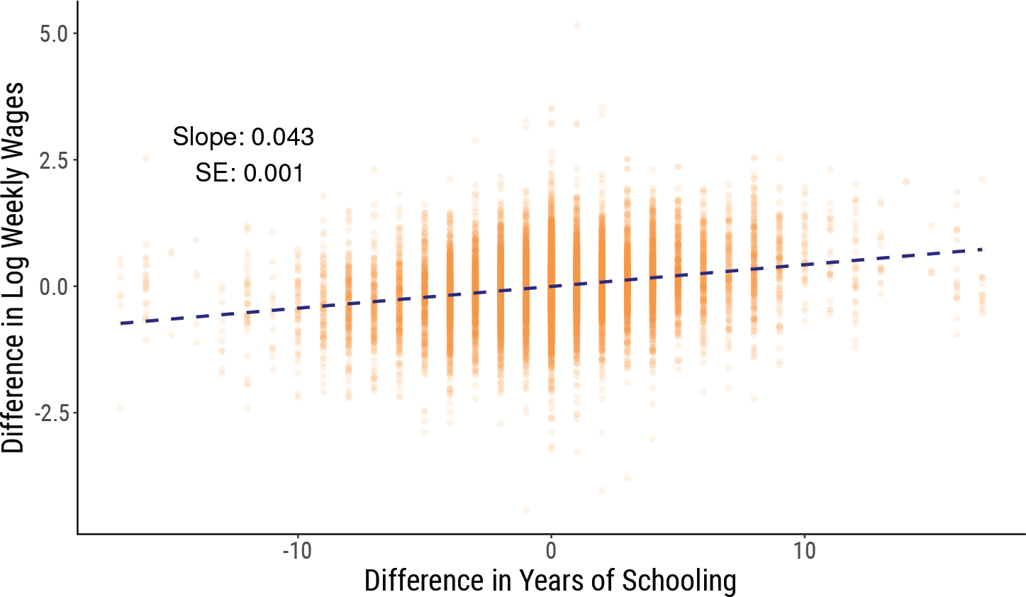
Figure 2 summarizes our main findings, plotting within-twins differences in earnings against within-twins differences in education: an additional year of schooling raises earnings by 0.043 log points or more than 4 percent. To estimate the return to education more formally, we turn to the regressions specified in Equations (1) and (2).
THE RETURN TO SCHOOLING IN THE EARLY TWENTIETH CENTURY
Notes: Data are from the pooled 1900–1940, 1910–1940, and 1920–1940 linked twins samples. The sample is restricted to wage and salary male workers with a weekly wage of at least $6, who worked a positive number of weeks in the previous year (1939), and who worked a positive number of hours in the preceding week, according to the 1940 census. The twins sample includes only twins who both fit our sample criteria. The best linear fit is shown. Robust standard errors are displayed.
Source: Ruggles et al. (Reference Ruggles, Flood, Goeken, Grover, Meyer, Pacas and Sobek2020).

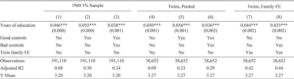
We estimate that the return to schooling was around 4 to 5 percent in the first half of the twentieth century.Footnote 21 Table 4 presents our results. Columns (1) to (3) are based on the 1940 1 percent census sample presented earlier in Table 3, while Columns (4) to (8) use the sample of linked twins. We compare the results from both datasets to determine whether the returns for the general population and twins are likely to differ. There are two takeaways from Table 4. First, the OLS coefficients are reasonably similar across the two datasets. The coefficients on years of education are nearly identical when comparing columns with the same set of covariates—no controls, exogenous controls, or exogenous and bad controls together. If the direction and magnitude of bias in the OLS results are similar for the two groups, then the actual return to education may also be similar for both populations. In either dataset, the estimated return is lowest when the bad controls are added. Of course, this should be viewed cautiously given the difficulty in interpreting regressions with bad controls (Angrist and Pischke Reference Angrist and Pischke2009). Second, the estimates are slightly smaller when attempting to address ability bias with family fixed effects. Our preferred model in Column (7) indicates a 4.4 percent increase in wages for each additional year of schooling on average, down from 5.0 or 5.6 percent in the pooled regressions, without or with the exogenous controls, respectively.Footnote 22 Again, this effect shrinks when the set of potentially endogenous controls are included in Column (8).
THE RETURN TO EDUCATION: BASELINE

Notes: All columns present regressions of the log of weekly earnings in 1939 on years of education, drawing on the 1940 census. In Columns (1), (2), and (3), we use a random 1 percent sample of the 1940 census. In Columns (4), (5), and (6), we turn to our linked sample of twin brothers, linking twins from the 1900, 1910, and 1920 censuses to 1940. In Columns (7) and (8), we include twin family fixed effects, forcing the comparisons of earnings and education to be between twin brothers. With the twin family fixed effects, the “good” controls—age, age-squared, race, and nativity—are subsumed because they cannot vary between twins. In all cases our sample is restricted to wage and salary male workers with a weekly wage of at least $6, who worked a positive number of weeks in the previous year (1939), and who worked a positive number of hours in the previous week. The twins sample includes only twins who both fit our sample criteria. Following Bailey et al. (Reference Bailey, Cole, Henderson and Massey2019), we use inverse propensity weights to adjust for observable differences between matched and unmatched people in our census linked sample. Robust standard errors (clustered at the twin-pair level in Columns (4) to (8)) are in parentheses.
*p < 0.1, **p < 0.05, ***p < 0.01
Source: Ruggles et al. (Reference Ruggles, Flood, Goeken, Grover, Meyer, Pacas and Sobek2020).
Our results paint a mixed picture regarding the direction of bias in naive OLS estimates. When predetermined controls are added, from Columns (1) to (2) and Columns (4) to (5), the point estimates increase in magnitude. This suggests that those with more schooling are negatively selected. However, the fixed effects coefficients are always smaller than the corresponding OLS results, which may instead hint at the more conventional story of positive selection.
Our findings suggest a lower return to schooling at mid-century than has been previously documented.Footnote 23 Clay, Lingwall, and Stephens (Reference Clay, Lingwall and Stephens2016), exploiting changes in CSLs during the first half of the twentieth century, estimate a return with a lower bound of 6.4 percent. Twins estimates from the late twentieth century, on the other hand, hover around 10 percent (Ashenfelter and Rouse Reference Ashenfelter and Rouse1998; Behrman and Rosenzweig Reference Behrman and Rosenzweig1999; Rouse Reference Rouse1999).Footnote 24 That our results differ from those in Clay, Lingwall, and Stephens (Reference Clay, Lingwall and Stephens2016) despite focusing on a similar period may not be surprising, as the group of compliers in the CSL “experiment” is likely to be different from ours. This difference could work in our favor as the use of twins allows for a direct comparison with the estimates for more recent cohorts, many of which are based on the twins approach. Such a comparison suggests that the value of schooling has increased over time. Goldin and Katz (Reference Goldin and Katz2007) show that the return to education was high in 1915, but collapsed thereafter before rising again in the late twentieth century. Our lower rates fit well with the middle part of the Goldin and Katz narrative.Footnote 25
Sensitivity Analysis
Three potential issues may distort our findings: imperfections in record linkage, measurement error in years of schooling, and any remaining differences between twins that are not accounted for by the twin-pair fixed effects. We address these concerns in turn and provide suggestive evidence that our estimates are unlikely to have been severely biased by these issues.
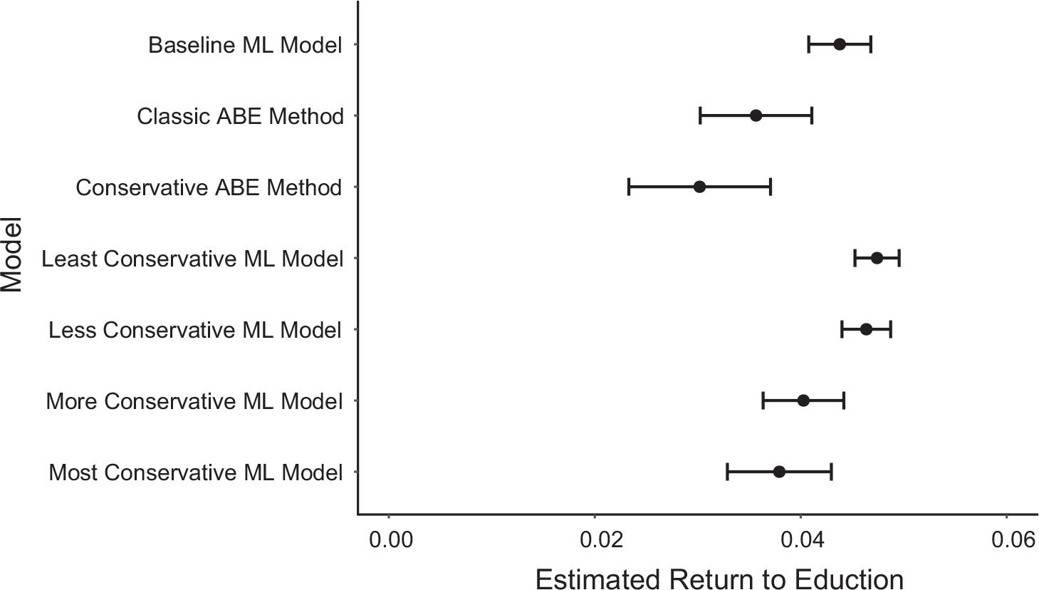
We begin with possible errors or imperfections in record linkage. Our estimated return to education is relatively stable across two of the most commonly used linking methods, as well as variants of those methods that alter the relative conservatism of the linking, which Abramitzky et al. (Reference Abramitzky, Boustan, Eriksson, Feigenbaum and Pérez2019) recommend as robustness tests for research using historical record linkage.
We use two methods to link twins. The first, presented throughout the article as our baseline, is the machine learning approach of Feigenbaum (Reference Feigenbaum2016) described earlier. The second is a simpler algorithmic approach, often referred to as ABE after Abramitzky, Boustan, and Eriksson (Reference Abramitzky, Boustan and Eriksson2012). The ABE method is similar to Long and Ferrie (Reference Long and Ferrie2013) and matches individuals with a deterministic procedure based on names, birthplace, and age. This procedure begins by searching for exact matches. If an exact match cannot be found, an age difference of one year is allowed, still requiring exact name and birthplace matching. The age window is then expanded to two years if a match still cannot be found. Both methods allow us to adjust the degree of conservatism. For the machine learning approach, this is done by varying the relative weight on false positives versus false negatives. For ABE, we report both the classic method and a more conservative version described in Abramitzky et al. (Reference Abramitzky, Boustan, Eriksson, Feigenbaum and Pérez2019) that further requires names to be unique within a five-year age band in both the base and target datasets as well as an exact match on age.
Figure 3 shows that our results are reasonably robust across all variants of the machine learning method, from the most to least conservative, as well as the classic and conservative ABE procedures. Even the result least in line with the rest—based on the much smaller sample of twins produced by the conservative ABE method—actually accords with our main conclusion, that the return to education in 1940 was positive but relatively low.Footnote 26
ROBUSTNESS OF THE ESTIMATED RETURN TO SCHOOLING IN THE EARLY TWENTIETH CENTURY ACROSS DIFFERENT LINKING METHODS
Notes: Data are from the pooled 1900–1940, 1910–1940, and 1920–1940 linked twins samples. We plot the return to education with 95 percent confidence intervals, based on robust standard errors clustered at the twin-pair level. The sample is linked with two methods: a machine learning approach (Feigenbaum Reference Feigenbaum2016) and an algorithmic approach (ABE after Abramitzky, Boustan, and Eriksson (Reference Abramitzky, Boustan and Eriksson2012), but similar to Long and Ferrie (Reference Long and Ferrie2013)). In the machine learning method, we vary the relative weight on false positives versus false negatives. For ABE, we report both the classic method and a more conservative version described in Abramitzky et al. (Reference Abramitzky, Boustan, Eriksson, Feigenbaum and Pérez2019). The sample is restricted to wage and salary male workers with a weekly wage of at least $6, who worked a positive number of weeks in the previous year (1939), and who worked a positive number of hours in the preceding week, according to the 1940 census. The twins sample includes only twins who both fit our sample criteria. Following Bailey et al. (Reference Bailey, Cole, Henderson and Massey2019), we use inverse propensity weights to adjust for observable differences between matched and unmatched people in our census linked sample.
Source: Ruggles et al. (Reference Ruggles, Flood, Goeken, Grover, Meyer, Pacas and Sobek2020).

While concerns with record linkage are specific to our setting, measurement error poses a common challenge in the twins literature.Footnote 27 Rouse (Reference Rouse1999), for example, finds that 8 to 12 percent of the variation in reported schooling across twins stems from errors. In the presence of measurement error, the within-twins estimator could potentially increase the noise-to-signal ratio and attenuate the estimated returns (Griliches Reference Griliches1979). This is particularly concerning in our setting, as the smaller returns we estimate compared with the present might simply reflect the bias due to measurement error rather than genuine differences in the value of schooling at different points in time. One solution, first introduced by Ashenfelter and Krueger (Reference Ashenfelter and Krueger1994), is to instrument each twin’s own reported years of schooling with the level of education that the other twin reports for them. However, the information required to implement this method—namely asking one twin their sibling’s years of education—is not available in the historical censuses.
As an alternative means of reducing the degree of measurement error, we focus on twins who completed key milestones in education. We assume that respondents can remember key events in the past more clearly—for instance, whether or not they finished high school or college. There may thus be less reporting error for those attaining these levels of education. To implement this, we narrow our sample to twin pairs where both members completed one of the following education levels exactly: common school graduate, high school graduate, college graduate, or five or more years of college. The subset of these twin pairs where each sibling achieved a different milestone provides the variation needed to identify the return to education.Footnote 28
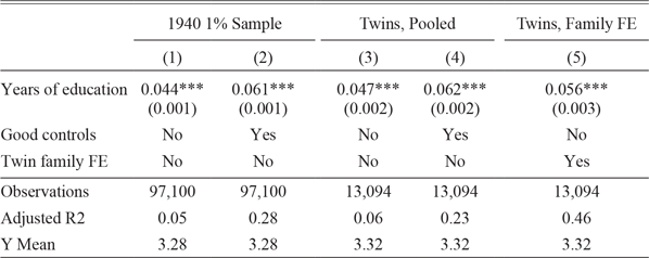
Using only twins who reached key milestones in education, we find rates of return that are similar to the baseline. Table 5 presents the results. The first four columns show the OLS results, where Columns (1) and (2) are based on the random sample of men in 1940 and Columns (3) and (4) are based on our twins sample. With these specifications, the point estimates are sensitive to the types of controls that are included—incorporating the good controls for age, race, and foreign-born status slightly increase the returns. Our preferred within-twins estimate in Column (5), although a bit larger than our findings in Table 4, still reinforces the conclusions from the preceding analysis: the return to schooling was positive at mid-century, but it was smaller than the returns for more recent cohorts.Footnote 29
THE RETURN TO EDUCATION: RESTRICTED TO SAMPLE WITH MILESTONE EDUCATION OUTCOMES

Notes: All columns present regressions of the log of weekly earnings in 1939 on years of education, drawing on the 1940 census. In Columns (1) and (2), we use a random 1 percent sample of the 1940 census but restrict to men with milestone years of education. In Columns (3) and (4), we turn to our linked sample of twin brothers, linking twins from the 1900, 1910, and 1920 censuses to 1940. In Column (5), we include twin family fixed effects, forcing the comparisons of earnings and education to be between twin brothers. With the twin family fixed effects, the “good” controls—age, age-squared, race, and nativity—are subsumed because they cannot vary between twins. In addition to the restrictions on our sample described in Table 4, we also restrict our sample to twins who both attained a milestone number of years of education: 8, 12, 16, or 16+. Following Bailey et al. (Reference Bailey, Cole, Henderson and Massey2019), we use inverse propensity weights to adjust for observable differences between matched and unmatched people in our census linked sample. Robust standard errors (clustered at the twin-pair level in Columns (3) to (5)) are in parentheses.
*p < 0.1, **p < 0.05, ***p < 0.01
Source: Ruggles et al. (Reference Ruggles, Flood, Goeken, Grover, Meyer, Pacas and Sobek2020).
Finally, we consider a major critique of using twins to estimate the return to schooling: even identical twins are not exactly the same. Any unobserved differences between twins will not be considered in the fixed effects model. Bound and Solon (Reference Bound and Solon1999), for example, make the case that there are differences within twin pairs before, during, and after birth. We provide suggestive evidence that such differences are unlikely to compromise our key findings.
For the within-twins estimates to be less biased than the OLS results, the endogenous variation in schooling within families need to be smaller than that between families. Since ability is unobserved, Ashenfelter and Rouse (Reference Ashenfelter and Rouse1998) and Bonjour et al. (Reference Bonjour, Cherkas, Haskel, Hawkes and Spector2003) assess this by taking several potential correlates of ability—such as marital status, self-employment, union coverage, test scores, spouse’s education—and comparing the associations between these covariates and schooling both within and between families. Using data from the late twentieth century, they find that the within-family correlations are much weaker than those between families, suggesting that much of the variation in unobserved ability is between families.
We follow the test in Ashenfelter and Rouse (Reference Ashenfelter and Rouse1998) and Bonjour et al. (Reference Bonjour, Cherkas, Haskel, Hawkes and Spector2003). We consider several potential correlates of ability: marital status, full-time employment status, the number of children one has, spouse’s years of education, and spouse’s labor force participation, all measured in 1940. The correlations between these characteristics and years of schooling are almost always statistically significant both within and between families (see Table A.6 in the Online Appendix). Nonetheless, the within-family correlations with years of schooling are always smaller in magnitude than the between-family correlations. This suggests that the rates of return based on the family fixed effects model may be less biased compared with estimates from the pooled OLS model.
This exercise, however, is not ideal in our setting for three reasons. First, many correlates of ability, such as test scores, are not available in our historical data. Second, while we can construct some correlates, an important outcome like self-employment cannot be used because our sample comprises only wage and salary workers. Third, although marital status and spousal education are reported, we simply do not know how strongly they are associated with ability in 1940. In the case of marriage, more than 75 percent of our linked twins were married by 1940 while the corresponding figure for the twins in Ashenfelter and Rouse (Reference Ashenfelter and Rouse1998) is lower at 64 percent. Since relatively more individuals were married in 1940, marital status could be less useful for distinguishing between people of different abilities historically.
We propose two ways of assessing the threat of unobservable differences between twin brothers, both of which are unique to our historical setting and data. Both tests, to some degree, rely on assumptions about how parents treat twin sons who show different levels of ability as children—investing more or less in the “more able” twin to equalize or exacerbate ability differences. After detailing the tests, we return to these assumptions.
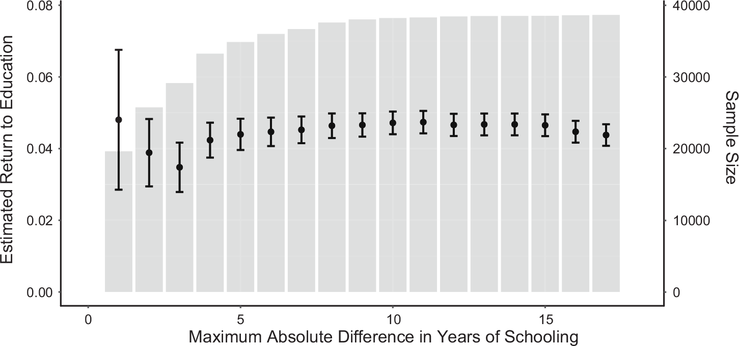
First, we gradually restrict the sample of twins to pairs with smaller differences in years of schooling and find little change in the estimated return to education. The smaller the gap in schooling, the more similar twins are likely to be in terms of unobserved ability. Consequently, the estimated rate of return may be less biased. Figure 4 plots the results from this exercise. Each marker represents the coefficient from a separate twin fixed effect regression, with 95 percent confidence intervals, and the maximum difference in schooling ranges from 1 to 17 years along the x-axis. Behind the point estimates, we plot the sample size corresponding to each regression. The return to schooling consistently hovers around 4 percent across the span of differences in years of schooling. This suggests that our baseline estimates are unlikely to be severely biased by within-twins differences in unobserved ability. Of particular interest are the results for twin pairs with education differences of four years or less—they comprise the majority of twin pairs as depicted by the sample size bars. With the smallest bandwidth of a year’s difference in schooling, the point estimate is 4.2 percent and is significant at the 1 percent level. The confidence intervals are very wide in this case, which is not surprising given the large amount of noise in wages within this narrow band hinted at in Figure 2. Nonetheless, the extreme upper bound of the 95 percent confidence interval is still slightly lower than the return to schooling in late twentieth-century twins studies.
THE RETURN TO SCHOOLING IS STILL POSITIVE EVEN AS THE SAMPLE IS NARROWED TO TWIN PAIRS WITH MORE SIMILAR YEARS OF SCHOOLING, FIXED EFFECTS RESULTS
Notes: Data are from the pooled 1900–1940, 1910–1940, and 1920–1940 linked twins datasets. Each marker represents the return to schooling from separate regressions of the log of weekly earnings in 1939 on years of education, with twin family fixed effects. The sample is restricted to wage and salary male workers with a weekly wage of at least $6, who worked a positive number of weeks in the previous year (1939), and who worked a positive number of hours in the preceding week. The sample size, given by the bars, ranges from 39,770 twins when the maximum difference in schooling is 17 years in either direction, to 20,670 twins when the maximum difference is only one year in either direction. Shown are 95 percent confidence intervals, based on robust standard errors clustered at the twin-pair level. Following Bailey et al. (Reference Bailey, Cole, Henderson and Massey2019), we use inverse propensity weights to adjust for observable differences between matched and unmatched people in our census linked sample.
Source: Ruggles et al. (Reference Ruggles, Flood, Goeken, Grover, Meyer, Pacas and Sobek2020).

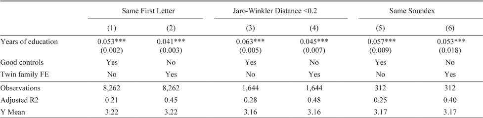
Second, we restrict our sample to pairs of twins who—even more than most twins—might be likely to receive identical treatment or resources from their parents. When we do so, we continue to find rates of return that are consistent with our baseline. Focusing on this subset of twins may help eliminate differences in the nurture aspect of unobserved ability. We propose using the similarity of first names as an indicator of parents’ intentions to treat their twins similarly. Online Appendix A.4 provides suggestive evidence that first names do carry valuable information on the intentions of parents: twins with more similar names are more likely to have the same school enrollment status in 1900, 1910, and 1920.Footnote 30 Names that are more similar may thus identify children who were raised with comparable resources and in similar environments. We use three measures of name similarity: first names that begin with the same letter, that have a Jaro-Winkler string distance of less than 0.2, or that belong to the same Soundex phonetic group.Footnote 31 Three subsets of twins are identified with these metrics, which we then use to re-estimate Equations (1) and (2). Table 6 presents the resulting coefficients. Though some subsamples are quite small, the fixed effects estimates in the even columns are broadly similar to the baseline.
THE RETURN TO EDUCATION: TWIN PAIRS WITH SIMILAR FIRST NAMES

Notes: All columns present regressions of the log of weekly earnings in 1939 on years of education, drawing on our linked sample of twin brothers, linking twins from the 1900, 1910, and 1920 censuses to 1940. We restrict the sample to pairs of twins who, based on their given names, we believe may be more likely to have been treated alike by their parents and families. In Columns (1) and (2), we limit the sample to twins whose first names start with the same letter. In Columns (3) and (4), we limit to twins whose first names are quite close in string distance. In Columns (5) and (6), we limit to twins whose first names have the same phonetic score (using Soundex). In the even columns, we include twin family fixed effects, forcing the comparisons of earnings and education to be between twin brothers. With the twin family fixed effects, the “good” controls—age, age-squared, race, and nativity—are subsumed because they cannot vary between twins. In all cases our sample is restricted to wage and salary male workers with a weekly wage of at least $6, who worked a positive number of weeks in the previous year (1939), and who worked a positive number of hours in the previous week. The twins sample includes only twins who both fit our sample criteria. Following Bailey et al. (Reference Bailey, Cole, Henderson and Massey2019), we use inverse propensity weights to adjust for observable differences between matched and unmatched people in our census linked sample. Robust standard errors clustered at the twin-pair level are in parentheses.
*p < 0.1, **p < 0.05, ***p < 0.01
Source: Ruggles et al. (Reference Ruggles, Flood, Goeken, Grover, Meyer, Pacas and Sobek2020).
While these two exercises strengthen our confidence in our twin-based findings, they require different but strong assumptions. When we compare twins with shrinking differences in actual education, we assume that the gap in education within a twin pair is informative of innate ability. The similar-name subsample analysis requires that names be informative of potential differences in parental investments. In both cases, the metrics—and our tests—may be distorted if parents respond endogenously to differences in ability observed between their children. Parents could respond by equalizing inputs across children, by investing disproportionately in the high-ability twin, or by investing more in the low-ability twin. In this same historical period, Parman (Reference Parman2015) found parents shifted educational investments to healthier siblings. If parents of twins respond similarly then the resulting differences in schooling, while possibly smaller, might not be indicative of smaller differences in unobserved ability. Parents who plan to treat twins identically—signalled with similar naming—could have their plans derailed by the reality of parenting. As we find in Online Appendix A.4, educational investments are more correlated for similarly named pairs. Generally, the weaker any endogenous parental responses, the cleaner these tests are and the more confident we can be in using the twins method to causally identify the return to education.
The Return to Education: Within or across Occupations?
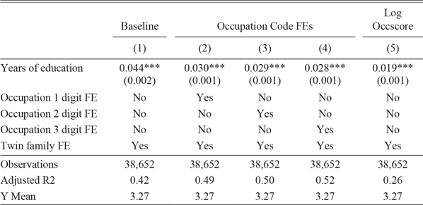
Education can translate into higher earnings in two key ways. First, more education could enable workers to work in “better” occupations. Second, within a given occupation, better educated workers may be more productive and thus earn more. Which channel is driving the return to schooling? To shed light on this, we add occupation fixed effects of varying coarseness to the twins specification to consider variation in earnings across occupations.
Table 7 presents the results from this exercise. Column (1) reproduces our baseline result—an additional year of education increases weekly earnings by 0.044 log points. Columns (2) to (4) include increasingly narrow fixed effects for occupations, based on the three-digit occupation code (occ1950) from IPUMS.Footnote 32 The return falls to 0.030 at the one-digit level, to 0.029 at the two-digit level, and to 0.028 at the three-digit level. About two-thirds of the return to education thus appears to stem from higher earnings within an occupation. This differs somewhat from Goldin and Katz (Reference Goldin and Katz2009), who perform a similar analysis using the 1915 Iowa sample and conclude that about half of the return to schooling is within occupations while the other half is between occupations.Footnote 33
THE RETURN TO EDUCATION: WITHIN OR ACROSS OCCUPATIONS?

Notes: Columns (1) to (4) present regressions of the log of weekly earnings in 1939 on years of education, drawing on our linked sample of twin brothers, linking twins from the 1900, 1910, and 1920 censuses to 1940. In Column (5), we use the same sample but take the log of occupation scores (using the standard IPUMS occscore variable) as the outcome. Column (1) duplicates our baseline results from Table 4. In Columns (2), (3), and (4), we add fixed effects for occupation, using the three-digit occupation code from IPUMS. The reduction in the return to education with the inclusion of these increasingly narrow occupation fixed effects suggests that some of the return to education in 1940 was driven by education changing (upgrading) occupation. But because the coefficient in Column (4) is still sizable (nearly two-thirds of the coefficient in Column (1)), there is also a substantial return to education within occupations. In all columns, we include twin family fixed effects, forcing the comparisons of earnings and education to be between twin brothers. Our sample is restricted to wage and salary male workers with a weekly wage of at least $6, who worked a positive number of weeks in the previous year (1939), and who worked a positive number of hours in the previous week. The twins sample includes only twins who both fit our sample criteria. Following Bailey et al. (Reference Bailey, Cole, Henderson and Massey2019), we use inverse propensity weights to adjust for observable differences between matched and unmatched people in our census linked sample. Robust standard errors clustered at the twin-pair level are in parentheses.
*p < 0.1, **p < 0.05, ***p < 0.01
Source: Ruggles et al. (Reference Ruggles, Flood, Goeken, Grover, Meyer, Pacas and Sobek2020).
Another way of showing that more schooling improves both the type of occupation and earnings within an occupation is to estimate the rate of return with occupation scores rather than earnings. Occupation scores, constructed by IPUMS based on the median earnings in 1950 for each occupation, are a common proxy for SES. These scores eliminate any variation within occupations. Twins with more education have higher occupation scores, as shown in Column (5) of Table 7, but the relative elasticity is lower than the results with earnings. This underscores that workers in 1940 benefited from education both via entry into better paying occupations and higher pay within occupations.Footnote 34
HETEROGENEITY IN THE RETURN TO EDUCATION
With the twins identification strategy and a large sample, we can estimate the return to schooling for different subsets of the population in 1940. This section considers two potential dimensions of heterogeneity: family status and immigration history. Does education enhance intergenerational mobility or facilitate assimilation among immigrants? We find suggestive evidence for the former but not the latter: there are higher returns to education for those whose fathers were farmers or had lower SES, but twins with more foreign-born grandparents had lower returns.
The Return to Education by Family Economic Status
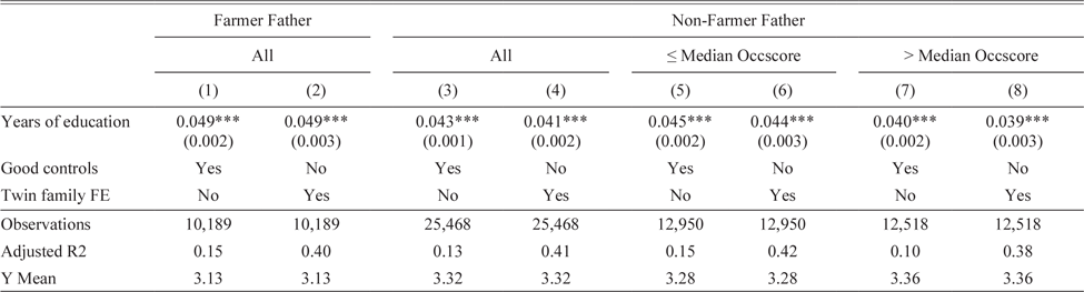
Schooling can weaken intergenerational economic persistence if the return to education is higher for children from lower SES families. We find higher returns for the sons of farmers and for sons whose fathers were in the bottom half of the SES distribution, but such differences are not large. Table 8 stratifies the sample of twins by the father’s occupation and SES and then estimates the return to education. Specifically, we split the sample into three groups: twin sons of farmers, twin sons with fathers in the bottom half of the occupation score distribution, and twin sons of fathers in the top half of the occupation score distribution. We separate out farmers for two reasons. First, farmers are the most common occupation category for fathers in our sample, which is not surprising given the declining but still-important place of agriculture in the U.S. economy during the early twentieth century. Second, we use the occupation scores of fathers to determine family SES. These scores may be especially weak indicators of SES for the large and highly varied category of farmers, which comprises positions ranging from sharecroppers and tenant farmers to those owning and farming large acres of land. Feigenbaum (Reference Feigenbaum2018) documents a large variance in actual earnings among farmers in 1915 Iowa but these farmers would all be assigned the same occupation score.
THE RETURN TO EDUCATION: HETEROGENEITY BY FATHER’S OCCUPATION AND SES

Notes: All columns present regressions of the log of weekly earnings in 1939 on years of education, drawing on our linked sample of twin brothers, linking twins from the 1900, 1910, and 1920 censuses to 1940. We split the data by the occupation and occupational status of the twins’ fathers. In the first two columns, we focus on twins whose fathers were farmers. In the remaining six columns, we focus on twins whose fathers were not farmers, splitting these twins by their fathers’ occupation scores at the median in Columns (5) and (6) versus Columns (7) and (8). In the even columns, we include twin family fixed effects, forcing the comparisons of earnings and education to be between twin brothers. With the twin family fixed effects, the “good” controls—age, age-squared, race, and nativity—are subsumed because they cannot vary between twins. Our sample is restricted to wage and salary male workers with a weekly wage of at least $6, who worked a positive number of weeks in the previous year (1939), and who worked a positive number of hours in the previous week. The twins sample includes only twins who both fit our sample criteria. Following Bailey et al. (Reference Bailey, Cole, Henderson and Massey2019), we use inverse propensity weights to adjust for observable differences between matched and unmatched people in our census linked sample. Robust standard errors clustered at the twin-pair level are in parentheses.
*p < 0.1, **p < 0.05, ***p < 0.01
Source: Ruggles et al. (Reference Ruggles, Flood, Goeken, Grover, Meyer, Pacas and Sobek2020).
Our results suggest that the return to education at mid-century was higher for sons from households lower on the SES ladder. This is consistent with the quantile IV results in Clay, Lingwall, and Stephens (Reference Clay, Lingwall and Stephens2016) that show a monotonic decline in returns by quantile. However, the point estimates in the even columns in Table 8 are not statistically different from each other. Our results may reflect the association between education level and the status of one’s father—on average, sons of farmers had 9 years of schooling in 1940 compared to 9.6 and 10.3 years for sons of non-farmer fathers below or above the median occupation score, respectively—although this relation is unlikely to be strong enough to explain the differences in Table 8.
The Return to Education by Family Immigration History
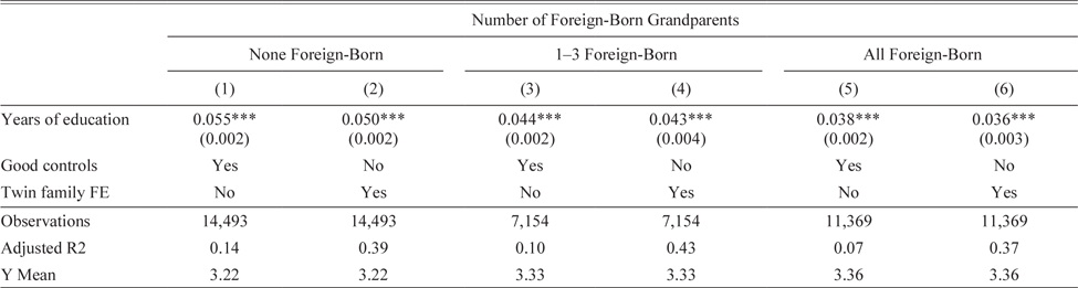
In the early twentieth century, proponents of mass education believed that the American school system could facilitate the assimilation of immigrants (Lleras-Muney and Shertzer Reference Lleras-Muney and Shertzer2015; Arington Reference Arington1991). Our sample contains very few foreign-born twins and twins with foreign-born parents. To determine if the return to schooling varies by immigration history, we thus focus on grandparents instead. Specifically, we divide white twins in our sample into three groups: those with no foreign-born grandparents, those with one to three foreign-born grandparents, and those whose grandparents are all foreign born.Footnote 35
The return to education was lower for children with more foreign-born grandparents. Table 9 presents the results. We focus on the even columns based on the twins fixed effects specification. The rates of return are highest for twins with four American-born grandparents and lowest for twins with four foreign-born grandparents.Footnote 36 Put differently, the labor market offers smaller rewards for twins with more recent family immigrant histories. Clay, Lingwall, and Stephens (Reference Clay, Lingwall and Stephens2016), exploiting variation in CSLs by state and cohort, also find higher returns among children with two American-born parents, compared to children with one or more foreign-born parents. While their results are somewhat imprecise, possibly because the first stage effect of compulsory schooling on the educational attainment of children with foreign-born parents is weak (Lleras-Muney and Shertzer Reference Lleras-Muney and Shertzer2015), they help reinforce our case that the return to schooling was lower for the children and grandchildren of the foreign born.Footnote 37
THE RETURN TO EDUCATION: HETEROGENEITY BY FAMILY IMMIGRATION HISTORY

Notes: All columns present regressions of the log of weekly earnings in 1939 on years of education, drawing on our linked sample of twin brothers, linking twins from the 1900, 1910, and 1920 censuses to 1940. We split the data by the family immigration history of twins. Because we observe twins in 1900, 1910, and 1920 in their childhood homes, we can use the census questions about the birthplaces of their parents’ parents to determine where their grandparents were born. The sample includes only white twins to avoid conflating race with grandparent and parent immigration histories, as nearly all African-American twins in the linked sample had four American-born grandparents. We also drop twin pairs from our baseline sample if both their mothers and fathers did not reside in their childhood household in the census. In the even columns, we include twin family fixed effects, forcing the comparisons of earnings and education to be between twin brothers. With the twin family fixed effects, the “good” controls—age, age-squared, race, and nativity—are subsumed because they cannot vary between twins. Our sample is restricted to wage and salary male workers with a weekly wage of at least $6, who worked a positive number of weeks in the previous year (1939), and who worked a positive number of hours in the previous week. The twins sample includes only twins who both fit our sample criteria. Following Bailey et al. (Reference Bailey, Cole, Henderson and Massey2019), we use inverse propensity weights to adjust for observable differences between matched and unmatched people in our census linked sample. Robust standard errors clustered at the twin-pair level are in parentheses.
*p < 0.1, **p < 0.05, ***p < 0.01
Source: Ruggles et al. (Reference Ruggles, Flood, Goeken, Grover, Meyer, Pacas and Sobek2020).
The lower return to schooling for third generation American twins could be explained by both segregation and language or cultural fluency. Residential segregation of immigrants was high in the early twentieth century (Eriksson and Ward Reference Eriksson and Ward2018). This implies that the children or grandchildren of immigrants were unlikely to attend the same schools as their peers with American-born grandparents. Consequently, the type and quality of schooling acquired by both groups may have been different, generating variation in the value of education across groups. This echoes the findings on the black-white gap in education returns (Card and Krueger Reference Card and Krueger1992; Carruthers and Wanamaker Reference Carruthers and Wanamaker2016, 2017). The lower returns could also reflect poorer language or cultural fluency. If the importance of formal education is mediated by language or culture, then those with a better command of English or knowledge of American culture will have relatively more effective (useful) units of human capital, all else equal. However, using an individual fixed effects model, Ward (2019b) finds that the return to English fluency in the early twentieth century was small compared to recent years. Residential segregation may thus be the more important of the two explanations.
Beyond differences in education returns by family status and immigration history, Online Appendix A.5 also explores if the return to schooling differs across cohorts and regions.Footnote 38 We find slightly larger returns to education for older cohorts and show that the value of education is fairly similar across regions.
THE RETURN TO EDUCATION ON OTHER OUTCOMES
While the primary goal of this article is to determine the weekly earnings return to education, additional years of schooling may also affect other outcomes. In this section, we leverage the same twins sample and approach to estimate the causal effect of education on a host of outcomes in 1940, including labor supply, migration, and family structure.
We begin by studying the effects of educational attainment on labor supply in 1940.Footnote 39 To do so, we expand our sample to include all linked twins. Table 10 presents our results. Panel A focuses on the extensive margin of labor supply by using several measures of employment status as the outcome. We find that twins with more schooling are slightly more likely to be employed (excluding relief work), but are less likely to be self-employed or to be employed in relief work. Panel B then studies other dimensions of labor supply that encompass both the extensive and intensive margins. Twins with more education were more likely to work full-time (defined as working more than 40 weeks in 1939), to work more weeks in a year, and to work more hours per week.
EFFECT OF EDUCATION ON ALTERNATIVE ECONOMIC OUTCOMES

Notes: All columns present regressions of employment (Panel A) or labor supply (Panel B) in 1940 on years of education, drawing on our linked sample of twin brothers, linking twins from the 1900, 1910, and 1920 censuses to 1940. In the even columns, we include twin family fixed effects, forcing the comparisons of outcomes and education to be between twin brothers. With the twin family fixed effects, the “good” controls—age, age-squared, race, and nativity—are subsumed because they cannot vary between twins. Our sample include all twins who were both linked to 1940, without further restrictions. Following Bailey et al. (Reference Bailey, Cole, Henderson and Massey2019), we use inverse propensity weights to adjust for observable differences between matched and unmatched people in our census linked sample. Robust standard errors clustered at the twin-pair level are in parentheses. We scale indicator dependent variables by 100 to simplify the interpretation of effects and standard errors.
*p < 0.1, ** p < 0.05, ***p < 0.01
Source: Ruggles et al. (Reference Ruggles, Flood, Goeken, Grover, Meyer, Pacas and Sobek2020).
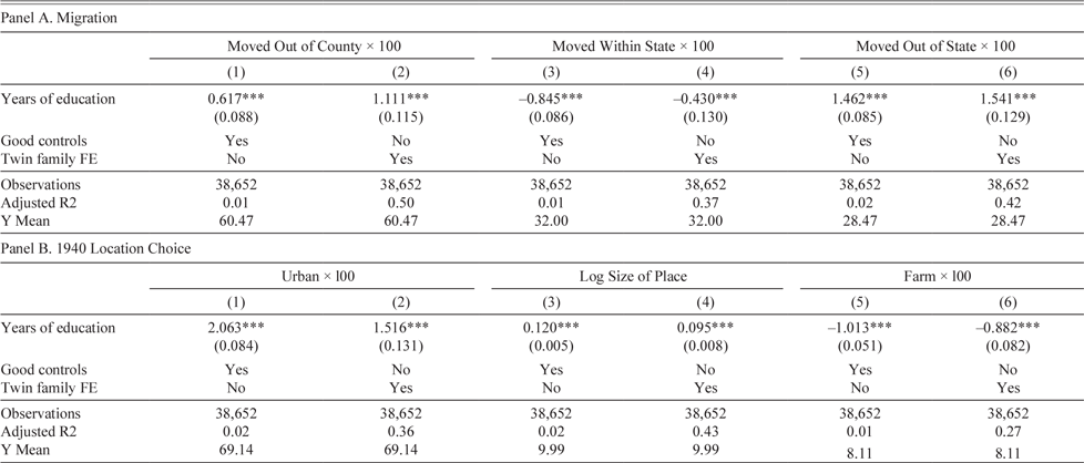
Education may have also influenced geographic mobility in the early twentieth century, as we show across a variety of measures in Table 11.Footnote 40 As before, we focus on the estimates with twin family fixed effects in the even columns. Those with more schooling have a higher propensity of leaving the counties they grew up in (Panel A, Column (2)), and these moves tend to be across states (Panel A, Column (6)). The association between education and geographic mobility during this period has been documented elsewhere in the literature.Footnote 41 Margo (1990), for example, argues that better-educated African Americans were more likely to move because schooling lowered the cost of migration through increasing one’s knowledge of distant opportunities or by enhancing a person’s ability to assimilate. The positive effect on cross-state migration is also consistent with Malamud and Wozniak (Reference Malamud and Wozniak2012), who exploit variation in college attainment due to draft avoidance during the Vietnam War to show that more years of college increase the odds of living outside one’s birth state. In addition to our migration results, we find that as adults, the twin with more schooling is more likely to reside in urban and more populous areas rather than on farms (Panel B).
EFFECT OF EDUCATION ON MIGRATION

Notes: All columns present regressions of migration (Panel A) or residential (Panel B) outcomes in 1940 on years of education, drawing on our linked sample of twin brothers, linking twins from the 1900, 1910, and 1920 censuses to 1940. In the even columns, we include twin family fixed effects, forcing the comparisons of outcomes and education to be between twin brothers. With the twin family fixed effects, the “good” controls—age, age-squared, race, and nativity—are subsumed because they cannot vary between twins. Our sample is restricted to wage and salary male workers with a weekly wage of at least $6, who worked a positive number of weeks in the previous year (1939), and who worked a positive number of hours in the previous week. The twins sample includes only twins who both fit our sample criteria. Following Bailey et al. (Reference Bailey, Cole, Henderson and Massey2019), we use inverse propensity weights to adjust for observable differences between matched and unmatched people in our census linked sample. Robust standard errors clustered at the twin-pair level are in parentheses. We scale indicator dependent variables by 100 to simplify the interpretation of effects and standard errors. Table A.11 in the Online Appendix replicates this analysis using the complete sample of linked twins and shows very similar results.
*p < 0.1, **p < 0.05, ***p < 0.01
Source: Ruggles et al. (Reference Ruggles, Flood, Goeken, Grover, Meyer, Pacas and Sobek2020).
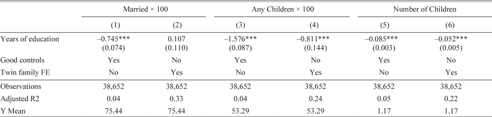
Finally, to examine differences in family structure, Table 12 implements Regressions (1) and (2), replacing the original wage outcome with three measures of family status in 1940: whether or not the twin is married, whether or not the twin has children in the household, and how many children are in the household, all measured in 1940. The fixed effects regressions in the even columns show no impact of schooling on the likelihood of marriage, although people with more schooling are less likely to have children and have fewer children overall.Footnote 42 The point estimates with the fertility outcomes, however, are small compared with the outcome means. In our sample, 53 percent have children, but another year of schooling lowers this by less than a percentage point. The effects are also small when compared to other shocks to human capital during this period. In a quite different context—the large scale school building program in the U.S. South targeted at African Americans from 1913 to 1932, known as the Rosenwald Rural Schools Initiative—Aaronson, Lange, and Mazumder (Reference Aaronson, Lange and Mazumder2014) find that African-American women who acquired more schooling had substantially lower fertility, particularly along the intensive margin.
EFFECT OF EDUCATION ON MARRIAGE AND FERTILITY

Notes: All columns present regressions of marriage or fertility outcomes in 1940 on years of education, drawing on our linked sample of twin brothers, linking twins from the 1900, 1910, and 1920 censuses to 1940. In the even columns, we include twin family fixed effects, forcing the comparisons of outcomes and education to be between twin brothers. With the twin family fixed effects, the “good” controls—age, age-squared, race, and nativity—are subsumed because they cannot vary between twins. Our sample is restricted to wage and salary male workers with a weekly wage of at least $6, who worked a positive number of weeks in the previous year (1939), and who worked a positive number of hours in the previous week. The twins sample includes only twins who both fit our sample criteria. Following Bailey et al. (Reference Bailey, Cole, Henderson and Massey2019), we use inverse propensity weights to adjust for observable differences between matched and unmatched people in our census linked sample. Robust standard errors clustered at the twin-pair level are in parentheses. We scale indicator dependent variables by 100 to simplify the interpretation of effects and standard errors. Table A.12 in the Online Appendix replicates this analysis using the complete sample of linked twins and finds very similar results for Columns (3) to (6). The marriage result in the full sample, however, does show a positive effect of education on the probability of being married.
*p < 0.1, **p < 0.05, ***p < 0.01
Source: Ruggles et al. (Reference Ruggles, Flood, Goeken, Grover, Meyer, Pacas and Sobek2020).
As documented in this section, the return to education in 1940 did not just accrue via more earnings. Twin siblings with more education were also likely to work more, to migrate (to cities and more populous places), and to have smaller families, although the effects on these alternative outcomes are often relatively small in size.
CONCLUSION
What was the return to schooling in mid-century America? Goldin and Katz (Reference Goldin and Katz2009) suggest that the returns were lower during this period in history compared with the earlier and later parts of the twentieth century. However, their conclusion is based on Mincerian correlations, leaving open the possibility that their results may be biased up or down by selection into education. Our article provides causal estimates of the return to schooling in 1940 and confirms that the returns were indeed lower relative to today. Given that income inequality was relatively lower in the middle of the twentieth century, the smaller returns we find are also consistent with the rise in income inequality from the 1980s onwards, much of which has been attributed to the growing skill premium (Goldin and Katz Reference Goldin and Katz2007).
Constructing a large linked sample of twins and exploiting within-twins variation in earnings and education, we estimate a return of around 4 percent in 1940. While positive, this is substantially smaller than the returns for more recent cohorts. We provide suggestive evidence that our results are not severely biased by imperfections in record linkage, measurement error in the years of schooling, or possible differences in ability within twin pairs.
Taking advantage of the large size of our dataset, we are also able to document heterogeneous effects of education for different subsets of the population. Those with more foreign-born grandparents, for instance, are observed to have a lower return to schooling.
Future research could proceed in several directions. First, quantifying the causal effect of education even further back in time could provide more evidence of the decline in the skill premium Goldin and Katz (Reference Goldin and Katz2009) trace before 1940. Second, estimating the historical returns in other countries could help shed light on whether the economic value of education in the United States during the mid-twentieth century was the exception or the norm. Third, within the U.S. labor market, our findings relate only to the return to education among men due to our method of linking individuals across censuses. The return to schooling for women remains to be studied, complementing work on the interaction of male and female labor supply at mid-century (Acemoglu, Autor, and Lyle Reference Acemoglu, Autor and Lyle2004). Although the lower rates of female labor force participation in the past complicates estimates of the return to education among women, the impact of schooling on earnings, occupation choice, labor supply, and other outcomes could offer important datapoints for scholars seeking to understand the labor market for women in this era.
Supplementary material
To view supplementary material for this article, please visit https://doi.org/10.1017/S0022050720000492