INTRODUCTION
Many countries throughout the world conduct an extensive safety evaluation on genetically modified (GM) crops before permitting their import for food and feed (König et al. Reference König, Cockburn, Crevel, Debruyne, Grafstroem, Hammerling, Kimber, Knudsen, Kuiper, Peijnenburg, Penninks, Poulsen, Schauza and Wal2004; Price & Underhill Reference Price and Underhill2013). Although there are procedural distinctions from country to country, a general consensus among regulatory authorities is that proof of genetically modified organism (GMO) safety can be accomplished under the concept of substantial equivalence (OECD 1993; FAO/WHO 1996; Codex Alimentarius Commission 2009). In accordance, a GM crop is compared to conventional non-GM crops in terms of key agronomic, phenotypic and compositional characteristics, or endpoints. Establishing substantial equivalence involves assessing their differences within the context of natural variation in conventional food crops (FAO/WHO 1996). Until recently, this has been accomplished via statistically comparing the GMO with its near-isogenic non-GM counterpart for each endpoint under the null hypothesis of ‘no difference’. A partial list of literature that executes such an assessment includes (Berman et al. Reference Berman, Harrigan, Riordan, Nemeth, Hanson, Smith, Sorbet, Zhu and Ridley2010; Zhou et al. Reference Zhou, Berman, Breeze, Nemeth, Oliveira, Braga, Berger and Harrigan2011; Herman et al. Reference Herman, Fast, Johnson, Sabbatini and Rudgers2013; Lepping et al. Reference Lepping, Herman and Potts2013; Lundry et al. Reference Lundry, Burns, Nemeth and Riordan2013; Privalle et al. Reference Privalle, Gillikin and Wandelt2013; Brink et al. Reference Brink, Chui, Cressman, Garcia, Henderson, Hong, Maxwell, Meyer, Mickelson, Stecca, Tyree, Weber, Zeng and Zhong2014; Venkatesh et al. Reference Venkatesh, Breeze, Liu, Harrigan and Culler2014). Non-significance is taken to mean there is no consequential difference between the two crops for a given endpoint. Unfortunately there are a series of flaws in this proof-of-difference approach. The most obvious is that the logic of statistical hypothesis testing does not allow one to interpret non-significance as evidence for the null hypothesis. At the same time, a significant difference does not necessarily imply practical importance. This shortcoming has been addressed in the literature listed above by a subsequent across-site comparison of the GMO mean against the data range and/or estimated percentiles derived from commercial non-GM references grown in the same study. However, such comparison suffers from its non-robustness to extreme data values. Further worsening the situation, the uncertainty of random sampling is not properly addressed. A less obvious but perhaps more important deficiency of the proof-of-difference approach is that it mitigates the producer's risk while failing to adequately control the consumer's risk. Under the context of substantial equivalence, the producer's risk is measured by the probability of concluding GMO is not comparable to non-GM crops when they are actually similar; the consumer's risk is quantified by the probability of accepting equivalence when certain features of GMO are severely altered beyond expectation. A difference test conducted at a fixed significance level (which is also the type I error rate) controls the producer's risk in GMO safety evaluation; it does not, however, facilitate transparent specification and straightforward management of the consumer's risk – a fact running contrary to the consumer's primary status in regulatory affairs. Some producers lessened their risk in safety studies even further by applying the false-discovery-rate adjustment originally developed for testing multiple endpoints in efficacy studies (Herman et al. Reference Herman, Fast, Johnson, Sabbatini and Rudgers2013; Lepping et al. Reference Lepping, Herman and Potts2013; Brink et al. Reference Brink, Chui, Cressman, Garcia, Henderson, Hong, Maxwell, Meyer, Mickelson, Stecca, Tyree, Weber, Zeng and Zhong2014). The systematic flaw of the test-of-difference approach has been outlined in a statistical framework by Berger (Reference Berger1982). Its problematic application in GMO safety evaluation was illustrated through numerical examples in Hothorn & Oberdoerfer (Reference Hothorn and Oberdoerfer2006).
A proof-of-equivalence approach aims to establish the similarity of two populations and essentially reverses the null and alternative hypotheses of the difference test. Significance in the equivalence test does indeed provide evidence of similarity and the significance level now represents the consumer's risk. Additionally, a non-significant result does not necessarily indicate a difference exists and the producer's risk can be minimized through increasing the sample size and optimizing the experimental design. Testing for equivalence is therefore the appropriate choice for GMO safety evaluation. Currently the GMO panel of the European Food Safety Authority (EFSA) mandates two sets of tests in the comparative assessment of a GM crop (EFSA 2010). Their difference tests detect potential changes from the near-isogenic non-GM counterpart and their equivalence tests evaluate GMO's similarity to commercial non-GM references. It is commonly agreed that the difference between GMO and references should be sufficiently small, but not necessarily zero, for one to conclude equivalence. A general expression for the equivalence hypotheses is given as
 $$ \hskip 22.5pt {H_0}:D(T,R) \ge \vartheta \quad v.\quad {H_1}:D(T,R) < \vartheta $$
Function D(T, R) represents a measure that quantifies the discrepancy of the GMO (test product) population with respect to the reference population. This measure is fully specified by population parameters rather than data-dependent statistics. When two populations are identical, D(T, R) = 0. The positive constant ϑ is a regulatory threshold for a given D(T, R). It defines the biological equivalence range tolerated by a regulatory authority. Schall & Williams (Reference Schall and Williams1996) refer to the equivalence measure D(T, R) together with its regulatory threshold ϑ as an equivalence criterion. EFSA (2010) and Van der Voet et al. (Reference Van der Voet, Perry, Amzal and Paoletti2011) recommend testing equivalence through comparison of intervals generated by standard statistical software without defining the equivalence criterion in terms of model parameters. As emphasized by Schall (Reference Schall, Blume and Midha1995a ), the critical step towards a compelling procedure for demonstrating equivalence is a clear specification of the equivalence criterion. Furthermore, it is unnecessary to restrict the choice of criteria according to the limitations of traditional statistical techniques as progress in modern statistical methodology already provides satisfactory paths forward. The present work focuses on developing equivalence criteria suitable for GMO safety evaluation. For the sake of brevity, statistical methodologies tailored to these criteria will be handled in separate publications.
Equivalence criteria have been much studied for the comparison between generic and brand name drugs. For decades, scientists from academia, government and industry have debated intensely over the measure of equivalence under a linear mixed model setting (Anderson & Hauck Reference Anderson and Hauck1990; Sheiner Reference Sheiner1992; Schall & Luus Reference Schall and Luus1993; Hauck & Anderson Reference Hauck and Anderson1994; Schall Reference Schall, Blume and Midha1995a ; Hauck et al. Reference Hauck, Chen, Hyslop, Patnaik, Schuirmann and Williams1996; Endrenyi & Midha Reference Endrenyi and Midha1998; Chen et al. Reference Chen, Patnaik, Hauck, Schuirmann, Hyslop and Williams2000; Dragalin et al. Reference Dragalin, Fedorov, Patterson and Jones2003; Haidar et al. Reference Haidar, Makhlouf, Schuirmann, Hyslop, Davit, Conner and Yu2008). This has led to a better understanding of issues related to the demonstration of bioequivalence, i.e. equivalence with respect to drug absorption. New bioequivalence criteria continue to appear as additional applications emerge (Chow et al. Reference Chow, Hsieh, Chi and Yang2010, Reference Chow, Endrenyi and Lachenbrunch2013; Kang & Chow Reference Kang and Chow2013). Nonetheless, there are remarkable differences between GMO safety evaluation and bioequivalence testing. From the biological aspect, in vivo bioequivalence studies of orally administered drugs intend to assess the difference between test and reference products at the individual subject level; in vitro bioequivalence studies of nasal sprays and aerosols intend to assess product differences across batches and canisters; GMO safety studies aim at evaluating the difference between GMO and references in the context of natural variation. From the design aspect, in vivo bioequivalence studies use cross-over designs and in vitro bioequivalence studies use completely randomized designs with sub-sampling; GMO safety studies typically use multi-site randomized complete block (RCB) designs. From the modelling aspect, a study on drug bioequivalence references one product; a study on GMO equivalence includes an assortment of non-GM commercial varieties for references. From the decision-making aspect, statistical significance is required for regulatory drug approval; non-significance in testing GMO equivalence does not lead directly to regulatory denial.
The present paper first introduces the linear mixed model employed by EFSA. The impact of genotype-by-site interaction, also known as G × E with E standing for environment, is then examined using results from several recent publications. Models with multiple variance components give rise to three types of distributions relevant for GMO safety evaluation. Equivalence criteria addressing each type of distribution are generated using two different machineries. The machinery of scaled average equivalence (SAE) compares the test product with the reference product by scaling their squared mean difference to the variability of the reference distribution. This machinery complies with the common practice of judging the GMO mean against percentiles of reference distributions. Its usage in assessing GMO equivalence also harmonizes with the current recommendation by the U.S. Food and Drug Administration (FDA) for in vivo bioequivalence studies (Davit et al. Reference Davit, Chen, Conner, Haidar, Kim, Lee, Lionberger, Maklouf, Nwakama, Patel, Schuirmann and Yu2012). The machinery of distribution-wise equivalence (DWE) judges the test product against the reference product via their entire distributions. It is useful for incorporating G × E. Furthermore, DWE criteria deliver straightforward interpretation regardless of whether G × E is present in the model. The criteria introduced here assess three ordered classes of equivalence. Their practical implications are investigated over an array of parameter values estimated from a real-world dataset. Finally, the present work provides new perspectives on issues surrounding G × E and makes recommendations on the choice of equivalence criteria for evaluating GMO safety.
MATERIALS AND METHODS
Experimental design and linear mixed models
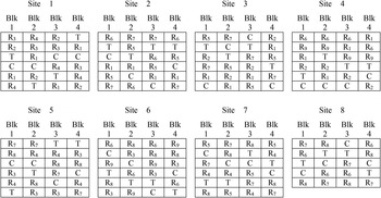
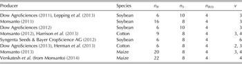
EFSA (2010) recommends that the field design for GMO safety evaluation contain a minimum of eight sites (n S ≥ 8) and a total of at least six reference varieties (n R ≥ 6) with a minimum of three reference varieties per site. The RCB design is typically implemented within each site, where GMO, its near-isogenic counterpart (control) and the selected references are randomized into field plots arranged in four blocks (n B(S) = 4). Table 1 presents the samples sizes employed by several major producers in the ag-biotech industry. Figure 1 illustrates a practical design where the allocation of references to site was taken from a safety study on GM cotton (Monsanto 2012; Harrison et al. Reference Harrison, Howard, Malven, Halls, Culler, Harrigan and Wolfinger2013), where the GMO and its control were grown at eight sites together with nine references. Each site contains three or four references.
An example of the field design for a GMO safety study. T, the GM crop; C, the non-GM near-isogenic counterpart; R 1~R 9, commercial non-GM references. Allocation of references to sites is taken from Harrison et al. (Reference Harrison, Howard, Malven, Halls, Culler, Harrigan and Wolfinger2013).

Sample sizes of field designs employed by the ag-biotech industry

n R , number of references; n S , number of sites; n B(S), number of blocks per site; ν, number of reference varieties per site.
Let Y ijl be the response of crop genotype i in block l at site j where i = 1,…, n R , T, C; j = 1,…, n S ; l = 1,…, n B(S). EFSA (2010) and Van der Voet et al. (Reference Van der Voet, Perry, Amzal and Paoletti2011) applied the following linear mixed model for testing equivalence:
 $${Y_{ijl}} = \left\{ {\matrix{ {{\mu _R} + {R_i} + {S_j} + B{{(S)}_{l(\,j)}} + {E_{ijl}}} & {i = 1, \ldots, {n_R}} \cr \hskip -2em {{\mu _T} + {S_j} + B{{(S)}_{l(\,j)}} + {E_{ijl}}} & \hskip -3.4em {i = T} \cr \hskip -2em {{\mu _C} + {S_j} + B{{(S)}_{l(\,j)}} + {E_{ijl}}} & \hskip -3.4em {i = C} \cr}} \right.$$
Because of natural variation among reference genotypes, Model (2) considers genotype as a treatment factor with both fixed and random levels. Parameters μ
R
, μT
and μ
C
correspond to the respective fixed effect of the reference, GMO and control genotype group. Effect R
i
from reference i is a normal random variable with mean zero and variance
 $\sigma _R^2 $
, i.e.
 ${R_i}\sim N(0,\sigma _R^2 )$
. It represents a super-population of reference genotype means centred at zero. Random effects corresponding to site and block nested within site are represented by
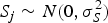 ${S_j}\sim N(0,\sigma _S^2 )$
and
 $B{(S)_{l(j)}}\sim N(0,\sigma _{B(S)}^2 )$
, respectively. The random error term
 ${E_{ijl}}\sim N(0,\sigma _E^2 )$
comprises plot-to-plot natural variation and variation due to sample processing and measurement. Random effects in Model (2) are mutually independent. The block-within-site term is usually kept in the model so as to fully represent the field design notwithstanding its trivial effect in comparison with the other variance components.
Terms representing G × E are customary in assessing GMO efficacy from field experiments. A classical G × E effect occurs when the difference between two genotypes experiences more variability than could be explained by a model without interaction. Historical studies on crop composition indicate that the effect of G × E could be significantly non-zero in some occasions (Oberdoerfer et al. Reference Oberdoerfer, Shillito, Beuckeleer and Mitten2005; Harrigan et al. Reference Harrigan, Stork, Riordan, Reynolds, Ridley, Masucci, MacIsaac, Halls, Orth, Smith, Wen, Brown, Welsch, Riley, McFarland, Pandravada and Glenn2007, Reference Harrigan, Glenn and Ridley2010; Zhou et al. Reference Zhou, Berman, Breeze, Nemeth, Oliveira, Braga, Berger and Harrigan2011). The ag-biotech industry viewed the absence of G × E in Model (2) as a fatal flaw and argued against the legitimacy of regulatory requirements on equivalence testing (Ward et al. Reference Ward, Nemeth, Brownie, Hong, Herman and Oberdoerfer2012). Van der Voet et al. (Reference Van der Voet, Perry, Amzal and Paoletti2012) attended to their criticism by examining the effect of G × E in an analysis-of-variance model containing fixed effects only. However, it is not clear how to connect results from two conflicting models and draw a cohesive conclusion on equivalence. This prompted the present work to pursue equivalence criteria under the more complex model given below.
 $$Y_{ijl} = \left\{ \matrix{ \matrix{{\mu _R} + {R_i} + {S_j} + G \times {S_{Rj}} \hfill\cr + R \times {S_{ij}} + B{{(S)}_{l(\,j)}} + {E_{ijl}}}\hfill & {i = 1, \ldots, {n_R}} \cr \hskip -2.6em {{\mu _T} + {S_j} + G \times {S_{Tj}}} \cr \hskip -3em + {B{{(S)}_{l(\,j)}} + {E_{ijl}},} & \hskip -3.5em {i = T} \cr \hskip -2.5em{{\mu _C} + {S_j} + G \times {S_{Cj}}} \cr \hskip -2.7em+ {B{{(S)}_{l(\,j)}} + {E_{ijl}},} &\hskip -3.5em {i = C} \cr} \right.$$
Model (3) accounts for G × E with two random terms: G × S and R × S. The interaction of genotype group with site is represented by the tri-variate normal random vector (G × S
Rj
G × S
Tj
G × S
Cj
)′ with mean (0 0 0)′ and covariance
 $\sigma _{G \times S}^2 {{\bf I}_3}$
, where I
3 denotes the 3 × 3 identity matrix. The interaction of reference genotypes with site is captured by the random effect
 $R \times {S_{ij}}\sim N(0,\sigma _{R \times S}^2 )$
. All random effects in Model (3) are mutually independent. Other linear mixed models that depict G × E in more intricate variance-covariance structures can be envisaged. The strength of Model (3) resides in its simplicity and interpretability. Note that when
 $\sigma _{G \times S}^2 = \sigma _{R \times S}^2 = 0$
, Model (3) reduces to Model (2).
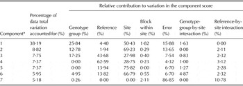
The safety implication of G × E has been questioned by Van der Voet et al. (Reference Van der Voet, Perry, Amzal and Paoletti2012) in their response to Ward et al. (Reference Ward, Nemeth, Brownie, Hong, Herman and Oberdoerfer2012). Recent publications provide consistent evidence against the ag-biotech industry's assertions on the absolute necessity of G × E in modelling crop composition. In particular, Harrison et al. (Reference Harrison, Howard, Malven, Halls, Culler, Harrigan and Wolfinger2013) represented the effect of G × E in a way similar to Model (3). To reduce the number of response variables, they processed the 51 compositional endpoints of a GM cotton through principal component analysis and then modelled the resulting scores of seven uncorrelated key components in a manner analogous to Model (3) except treating the effect of genotype group as random. Table 2 summarizes the relative contribution of random effects to data total variation. This result is in agreement with previous recognition that site, reference genotype and error terms are the major sources of variation in crop composition, while blocking within site has a minor effect (Berman et al. Reference Berman, Harrigan, Riordan, Nemeth, Hanson, Smith, Sorbet, Zhu and Ridley2010; Harrigan et al. Reference Harrigan, Glenn and Ridley2010; Van der Voet et al. Reference Van der Voet, Perry, Amzal and Paoletti2011; Shewry et al. Reference Shewry, Hawkesford, Piironen, Lampi, Gebruers, Boros, Andersson, Åman, Rakszegi, Bedo and Ward2013). Contribution of the two G × E terms to the total variation was much smaller than Ward et al. (Reference Ward, Nemeth, Brownie, Hong, Herman and Oberdoerfer2012) speculated, ranging from 0% in the primary component (accounting for 38% of data total variation) to 11% in the seventh largest component (accounting for 5% of data total variation). Moreover, the negligible effect of G × E has been reported from variance component analyses on the principal components of GM soybean (Harrigan et al. Reference Harrigan, Culler, Culler, Breeze, Berman, Halls and Harrison2013) and on the compositional endpoints of GM maize (Venkatesh et al. Reference Venkatesh, Breeze, Liu, Harrigan and Culler2014). Results from these three separate studies indicate that the non-zero significance of G × E observed in the past is unlikely to be present to a practically important degree.
An example for the relative contribution of various sources to the total variation in crop composition (Harrison et al. Reference Harrison, Howard, Malven, Halls, Culler, Harrigan and Wolfinger2013)
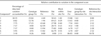
* Variance components were estimated from scores corresponding to seven key components in principal component analysis on 51 compositional endpoints. The seven components cumulatively accounted for 80% of the total variation of the compositional data.
Natural-log transformation before fitting the linear model to compositional endpoints is suggested by EFSA (2010). This parallels the recommendation by FDA (2001, 2003c ) in bioequivalence studies. To aid the interpretation of equivalence criteria, it is helpful to review two properties that connect parameters of the log-normal distribution, i.e. normal distribution on the log scale, to the original data scale.
-
Property 1: A positive random variable X is said to follow a log-normal distribution if Ln(X)~N(μ, σ 2). The geometric mean of X is exp(μ), which is also the median of X. The ratio of the geometric mean (median) for two log-normal random variables,
 $Ln({X_1})\sim N({\mu _1},\sigma _1^2 )$
and
$Ln({X_2}) $
$ \sim N({\mu _2},\sigma _2^2 )$
, is exp(μ
1 − μ
2).
-
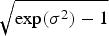
Property 2: The coefficient of variation (CV) of X is
$\sqrt {\exp ({\sigma ^2}) - 1} $
.



Equivalence criteria
It is articulated by EFSA (2010) that ‘statistical analysis of data from the experiments for comparative risk assessment is mainly concerned with studying the average difference and the average equivalence (AE) over sites. Here, the term ‘average equivalence’ is adopted in the sense used in the drug testing literature’. The AE criterion used in regulating drugs (FDA 2001, 2003a , b , c ; EMA 2010) corresponds to the following hypotheses:
 $$\hskip 9pt {H_0}:{({\mu _T} - {\mu _R})^2} \ge {\vartheta _{AE}}\quad v.\quad {H_1}:{({\mu _T} - {\mu _R})^2} < {\vartheta _{AE}}$$
The equivalence limit (EL) for (μ T − μ R )2 is fixed at Δ AE (ϑ AE , σ 2) = ϑ AE . The FDA sets ϑ AE = [Ln(1.25)]2 for in vivo bioequivalence studies and ϑ AE = [Ln(0.9)]2 for in vitro bioequivalence studies. The AE criterion is deficient for GMO safety evaluation in several ways. First, using [Ln(1.25)]2 or [Ln(0.9)]2 as the one-size-fits-all EL for testing GMO lacks scientific justification. Second, explicit ELs are difficult, if not impossible, to specify for the large number of compositional endpoints (Hothorn & Oberdoerfer Reference Hothorn and Oberdoerfer2006). Third, the AE criterion fails to consider natural variation.
The concept of substantial equivalence suggests comparing (μ T − μ R )2 to an EL that accounts for natural variation. Hypotheses (1) are rather abstract. Equivalence criteria to be introduced henceforth can all be re-expressed in the following form.
 $$\eqalign{&{H_0}:{({\mu _T} - {\mu _R})^2} \ge \Delta (\vartheta, {{\bf \sigma} ^2})\quad v.\cr\quad &{H_1}:{({\mu _T} - {\mu _R})^2} \lt \Delta (\vartheta, {{\bf \sigma} ^2})}$$
Function Δ(·) represents the EL for (μ
T
− μ
R
)2. Its formulation is derived from one's choice of D(T, R). There are two arguments for Δ(·): constant ϑ is the regulatory threshold for D(T, R); symbol σ
2 denotes the vector of variances in the linear mixed model. A practical interpretation of Hypotheses (4) is that GMO and references are deemed equivalent when their absolute mean difference is less than
 $\sqrt {\Delta (\vartheta, {{\bf \sigma} ^2})} $
. Appendix 1 conducts a brief survey on general strategies for developing equivalence criteria. The SAE and DWE machineries employ the collective strategies of ‘moment-based’, ‘reference-scaled’, ‘aggregated’, ‘non-symmetrical’ and ‘univariate’. They both demand specification of the GMO and reference distributions. It is important to recognize that there are three types of distributions relevant for testing GMO equivalence under Models (2) and/or (3): the super distributions of reference genotype means and GMO mean; the conditional distributions of references and GMO at the site and block level; the marginal distributions of references and GMO across sites and blocks. Comparing super distributions, in particular
 $N({\mu _R},\sigma _R^2 )$
with μ
T
, may seem enticing at first. Nonetheless, EFSA (2010) advocates checking GMO equivalence within individual sites. This, in essence, assesses equivalence on the basis of conditional distributions. Recall that traditional GMO safety evaluation accounts for natural variation by judging, across sites, the GMO mean against the data range and/or estimated percentiles from in-study references. This corresponds to assessing equivalence based on the marginal distribution of the references. Both conditional and marginal distributions have been involved in testing bioequivalence. The FDA currently considers conditional distributions (at the individual subject level) for in vivo bioequivalence studies and marginal distributions (across batches and canisters) for in vitro bioequivalence studies (FDA 2003a
,
c
; Davit et al.
Reference Davit, Chen, Conner, Haidar, Kim, Lee, Lionberger, Maklouf, Nwakama, Patel, Schuirmann and Yu2012). Also, veterinary medicines are often administered to food-producing animals on a population level via feed or water; marginal inference is more meaningful there (Toutain & Koritz Reference Toutain and Koritz1997). In order to thoroughly explore the options for assessing GMO equivalence, the present work operated the SAE and DWE machineries on super, conditional and marginal distributions.
Scaled average equivalence
The SAE machinery tunes the EL for (μ T − μ R )2 proportionally to the variance of the reference distribution. Due to the rising awareness of random effects in linear models, scaling has gradually been recognized as a sensible alternative to the AE criterion for in vivo bioequivalence studies on highly variable drugs (Boddy et al. Reference Boddy, Snikeris, Kringle, Wei, Oppermann and Midha1995; Midha et al. Reference Midha, Rawson and Hubbard1997; Haidar et al. Reference Haidar, Makhlouf, Schuirmann, Hyslop, Davit, Conner and Yu2008; EMA 2010; Schall & Endrenyi Reference Schall and Endrenyi2010). Its acceptance by the FDA was made official in 2012 (Davit et al. Reference Davit, Chen, Conner, Haidar, Kim, Lee, Lionberger, Maklouf, Nwakama, Patel, Schuirmann and Yu2012). Because SAE focuses on comparison of the mean difference and does not permit a straightforward incorporation of G × E, the three SAE criteria introduced here are expressed in terms of parameters for Model (2) only. Impact of G × E on GMO safety evaluation is investigated via the DWE machinery assuming the more complex Model (3).
Reference genotype is a major source of natural variation for many endpoints measured in crop safety evaluation (Van der Voet et al. Reference Van der Voet, Perry, Amzal and Paoletti2011; Harrison et al. Reference Harrison, Howard, Malven, Halls, Culler, Harrigan and Wolfinger2013; Shewry et al. Reference Shewry, Hawkesford, Piironen, Lampi, Gebruers, Boros, Andersson, Åman, Rakszegi, Bedo and Ward2013; also see Table 2). The concept of substantial equivalence suggests that reference-to-reference variability should be used when assessing GMO. Van der Voet et al. (Reference Van der Voet, Perry, Amzal and Paoletti2011) consider ‘appropriate percentiles (e.g. 2·5 and 97·5) of the distribution of reference variety characteristics’ as the limits for GMO's relative deviation from the overall mean of references. Accordingly, Kang & Vahl (Reference Kang and Vahl2014) proposed the following hypotheses under Model (2).
 $$\eqalign{&{H_0}:{\mu _T} - {\mu _R} \le {z_{0.025}}{\sigma _R}\quad {\rm or}\quad {\mu _T} - {\mu _R} \ge {z_{0.975}}{\sigma _R}\quad v.\quad \cr &{H_1}:{z_{0.025}}{\sigma _R} \lt {\mu _T} - {\mu _R} \lt {z_{0.975}}{\sigma _R}}$$
Constants z 0.025 = −1.96 and z 0.975 = 1.96 are the 2·5th and 97·5th percentiles of N(0,1). By symmetry of N(0,1), z 0.975 = −z 0.025. To be consistent with Form (1), the above hypotheses can be expressed more concisely as
 $$\eqalign{&{H_0}:\displaystyle{{{{({\mu _T} - {\mu _R})}^2}} \over {\sigma _R^2}} \ge z_{0.975}^2 \quad v.\quad \cr &{H_1}:\displaystyle{{{{({\mu _T} - {\mu _R})}^2}} \over {\sigma _R^2}} \lt z_{0.975}^2}$$
This reveals that an SAE criterion with
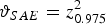 ${\vartheta _{SAE}} = z_{0.975}^2 $
has been employed. Because the equivalence measure in Hypotheses (5) scales (μ
T
− μ
R
)2 to the variance for the super population of reference genotype means, equivalence defined by H
1 of Hypotheses (5) is referred to as ‘SAE-S’. Although more biological support is needed to back up the decision on the regulatory threshold, the current work focused on the equivalence measure and tentatively assumed that
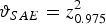 ${\vartheta _{SAE}} = z_{0.975}^2 $
is a reasonable choice. Hypotheses (5) can be converted to Hypotheses (4) with
 $$ \hskip 57pt {\Delta _{SAE - S}}({\vartheta _{SAE}},{{\bf \sigma} ^2}) = z_{0.975}^2 \sigma _R^2 $$
According to Property 1 of log-normal distributions, the SAE-S criterion considers GMO equivalent to references, with respect to a key compositional endpoint, if the ratio of their geometric means, i.e. exp(μ T − μ R ), is between exp(−z 0.975 σ R ) and exp(z 0.975 σ R ).
Hypotheses (5) conforms to the concept of substantial equivalence when
 $\sigma _R^2 $
dominates natural variation. For endpoints whose
 $\sigma _R^2 $
is considerably smaller than
 $\sigma _E^2 $
, i.e.
 $\sigma _R^2 \ll \sigma _E^2 $
, scaling leads to low ELs which demand (μ
T
− μ
R
)2 to be near zero. However, this is in conflict with the concept of substantial equivalence. Responses from the same genotype grown at different field plots at the same site tend to deviate from μ
R
; but those values are all considered safe. It is then desirable to incorporate
 $\sigma _E^2 $
into GMO testing. Kang & Vahl (Reference Kang and Vahl2014) propose the following SAE criterion.
 $$\eqalign{&{H_0}:\displaystyle{{{{({\mu _T} - {\mu _R})}^2}} \over {\sigma _R^2 + \sigma _E^2}} \ge z_{0.975}^2 \quad v.\quad \cr &{H_1}:\displaystyle{{{{({\mu _T} - {\mu _R})}^2}} \over {\sigma _R^2 + \sigma _E^2}} \lt z_{0.975}^2}$$
The scaling in Hypotheses (6) utilizes
 $\sigma _R^2 + \sigma _E^2 $
, the variance for the conditional distribution of references at a given site and block. Equivalence depicted by H
1 of Hypotheses (6), referred to as ‘SAE-C’, complies with Van der Voet et al. (Reference Van der Voet, Perry, Amzal and Paoletti2011) by choosing the 2·5th and 97·5th percentiles of the conditional distribution of references as the ELs for μ
T
. It was noticed that the average bioequivalence of a highly variable drug is scaled to the within-subject variance of the reference drug in the cross-over design (Haidar et al.
Reference Haidar, Makhlouf, Schuirmann, Hyslop, Davit, Conner and Yu2008; Davit et al.
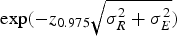
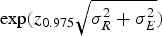
Reference Davit, Chen, Conner, Haidar, Kim, Lee, Lionberger, Maklouf, Nwakama, Patel, Schuirmann and Yu2012). Modelling-wise, sites and blocks in the multi-site RCB design operate analogously to human subjects in the cross-over design. The SAE-C criterion therefore harmonizes with the SAE criteria currently employed in drug studies. Converting Hypotheses (6) into the form of Hypotheses (4) yields
 $$ \hskip 42pt {\Delta _{SAE - C}}({\vartheta _{SAE}},{{\bf \sigma} ^2}) = z_{0.975}^2 (\sigma _R^2 + \sigma _E^2 )$$
For log-transformed data, the SAE-C criterion deems GMO equivalent to references if the ratio of their geometric means is between
 $\exp ( - {z_{0.975}}\sqrt {\sigma _R^2 + \sigma _E^2} )$
and
 $\exp ({z_{0.975}}\sqrt {\sigma _R^2 + \sigma _E^2} )$
. Note that Δ
SAE
−
C
(ϑ
SAE
,
σ
2) ≈ Δ
SAE−S
(ϑ
SAE
,
σ
2) when
 $\sigma _R^2 \gg \sigma _E^2 $
. Hypotheses (6) thus unifies with Hypotheses (5) when variability of the error term is trivial.
Environment, i.e. site, is another major contributor to crop natural variation (Berman et al.
Reference Berman, Harrigan, Riordan, Nemeth, Hanson, Smith, Sorbet, Zhu and Ridley2010; Harrigan et al.
Reference Harrigan, Glenn and Ridley2010; Harrison et al. Reference Harrison, Howard, Malven, Halls, Culler, Harrigan and Wolfinger2013; Van der Voet et al.
Reference Van der Voet, Perry, Amzal and Paoletti2011; also see Table 2). A literature search on GMO safety evaluation revealed a consensus that the EL for the GMO mean could be based on the marginal distribution of references across sites (e.g. Berman et al.
Reference Berman, Harrigan, Riordan, Nemeth, Hanson, Smith, Sorbet, Zhu and Ridley2010; Zhou et al.
Reference Zhou, Berman, Breeze, Nemeth, Oliveira, Braga, Berger and Harrigan2011; Herman et al.
Reference Herman, Fast, Johnson, Sabbatini and Rudgers2013; Lepping et al.
Reference Lepping, Herman and Potts2013; Lundry et al.
Reference Lundry, Burns, Nemeth and Riordan2013; Privalle et al.
Reference Privalle, Gillikin and Wandelt2013; Brink et al.
Reference Brink, Chui, Cressman, Garcia, Henderson, Hong, Maxwell, Meyer, Mickelson, Stecca, Tyree, Weber, Zeng and Zhong2014; Venkatesh et al.
Reference Venkatesh, Breeze, Liu, Harrigan and Culler2014). Under Model (2), the marginal reference distribution has a variance of
 $\sigma _R^2 + \sigma _S^2 + \sigma _{B(S)}^2 + \sigma _E^2 $
. Assessing GMO substantial equivalence can then be carried out by testing the following hypotheses.
 $$\eqalign{&{H_0}:\displaystyle{{{{({\mu _T} - {\mu _R})}^2}} \over {\sigma _R^2 + \sigma _S^2 + \sigma _{B(S)}^2 + \sigma _E^2}} \ge z_{0.975}^2 \quad v.\quad \cr &{H_1}:\displaystyle{{{{({\mu _T} - {\mu _R})}^2}} \over {\sigma _R^2 + \sigma _S^2 + \sigma _{B(S)}^2 + \sigma _E^2}} \lt z_{0.975}^2}$$
Equivalence depicted by H 1 of Hypotheses (7) is referred to as ‘SAE-M’. Its EL for (μ T − μ R )2 is
 $$ \hskip 15pt {\Delta _{SAE - M}}({\vartheta _{SAE}},{{\bf \sigma} ^2}) = z_{0.975}^2 (\sigma _R^2 + \sigma _S^2 + \sigma _{B(S)}^2 + \sigma _E^2 )$$
The SAE-M criterion complies with Van der Voet et al. (Reference Van der Voet, Perry, Amzal and Paoletti2011) by taking the 2·5th and 97·5th percentiles of the marginal distribution of references as the ELs for μ
T
. It is worthwhile to cite EFSA (2010) that ‘When the natural variation [
 $\sigma _R^2 $
] is very small or zero, and the calculated equivalence limits are considered by experts to have little practical relevance, external data may be used to establish new equivalence limits.’ Hong et al. (Reference Hong, Fisher, Sult, Maxwell, Mickelson, Kishino and Locke2014) estimated percentiles for the marginal distribution of references from historical data. When these data are large enough to ignore the uncertainty in estimation, establishing ELs from this external information can be viewed as implementing the SAE-M criterion where the reference mean and variances are derived from historical data. However, such an approach is not as reliable as directly testing Hypotheses (7) from in-study references because historical data may lose relevance over time. For log-transformed data, the SAE-M criterion considers GMO equivalent to references if the ratio of their geometric means falls between
 $\exp ( - {z_{0.975}}\sqrt {\sigma _R^2 + \sigma _S^2 + \sigma _{B(S)}^2 + \sigma _E^2} )$
and
 $\exp ({z_{0.975}}\sqrt {\sigma _R^2 + \sigma _S^2 + \sigma _{B(S)}^2 + \sigma _E^2} )$
. When
 $\sigma _R^2 \gg \sigma _S^2 + $
 $\sigma _{B(S)}^2 + \sigma _E^2 $
, Δ
SAE
−
M
(ϑ
SAE
,
σ
2) ≈ Δ
SAE
−C
(ϑ
SAE
,
σ
2) ≈ Δ
SAE
−S
(ϑ
SAE
,
σ
2) and Hypotheses (5–7) reconcile.
Noticeably ELs of the three SAE criteria are weighted sums of mixed model variance components. The SAE-S criterion places zero weight on
 $\sigma _S^2 + \sigma _{B(S)}^2 $
and
 $\sigma _E^2 $
. It depicts equivalence in the most stringent manner. The SAE-C criterion broadens Δ(·) by placing positive weight on
 $\sigma _E^2 $
. The SAE-M criterion further broadens Δ(·) by assigning positive weight to
 $\sigma _E^2 $
and
 $\sigma _S^2 + \sigma _{B(S)}^2 $
. Inspection of these ELs revealed the following inequalities.
 $$ \hskip 40pt {\Delta _{SAE - S}}({\vartheta _{SAE}},{{\bf \sigma} ^2}) < {\Delta _{SAE - C}}({\vartheta _{SAE}},{{\bf \sigma} ^2}) < {\Delta _{SAE - M}}({\vartheta _{SAE}},{{\bf \sigma} ^2})$$
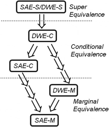
This organizes the H 1 parameter spaces of the SAE criteria according to a hierarchical order. Consequently, SAE-S implies SAE-C and SAE-C implies SAE-M (Fig. 2).
Logical hierarchy in equivalences at ϑ DWE = ϑ SAE − 1under Model (2).

Distribution-wise equivalence
The comments from the ag-biotech industry on the EFSA guidance plead for an equivalence criterion to take into account G × E (Ward et al. Reference Ward, Nemeth, Brownie, Hong, Herman and Oberdoerfer2012). This prompted the present work to explore equivalence criteria under Model (3). Incorporating the two G × E terms in this model requires the statistical principle of judging two products based on their entire distributions instead of their means only. The DWE machinery was originally introduced to bioequivalence testing in order to guard against subject-by-drug interaction (Anderson & Hauck Reference Anderson and Hauck1990; Sheiner Reference Sheiner1992; Schall & Luus Reference Schall and Luus1993; Hauck & Anderson Reference Hauck and Anderson1994; Schall Reference Schall, Blume and Midha1995a ). In the context of a clinical cross-over design, it created the individual bioequivalence and population bioequivalence criteria for comparing test and reference products based on their conditional distributions (at the individual subject level) and marginal distributions (across study subjects), respectively. These two criteria were once thought to supplant the AE criterion for in vivo bioequivalence studies (Endrenyi & Midha Reference Endrenyi and Midha1998). As concerns on subject-by-drug interaction attenuated over time (Endrenyi et al. Reference Endrenyi, Taback and Tothfalusi2000; Hsuan Reference Hsuan2000; Zariffa et al. Reference Zariffa, Patterson, Boyle and Hyneck2000), the FDA dismissed DWE criteria from their final guidance for in vivo bioequivalence testing (FDA 2003b ). Nevertheless, the DWE machinery should not be excluded from other areas of application. For example, FDA (2003a , c ) recommends in vitro studies on nasal products to implement the population bioequivalence criterion.
The usefulness of DWE does not reside only in its capability to handle interaction terms. Dragalin et al. (Reference Dragalin, Fedorov, Patterson and Jones2003) identified that its machinery generates equivalence measures linearly related to the Kullback–Leibler (KL) divergence, a well-known measure of the distance between two distributions in probability and information theories. For instance, the commonly practiced likelihood maximization aims at minimizing the KL divergence between the presumed model and the observed data (Section 13.2 of Pawitan Reference Pawitan2001). A DWE criterion can then be interpreted, in general, as deeming the test and reference products equivalent when the distance between their distributions is within the regulatory threshold. Because the KL divergence is invariant to monotone transformations of data, the interpretation of DWE is not restricted to the original data scale as long as there exists a monotone transformation (including but not limited to the log function) satisfying the normality assumption in the linear mixed model. Such a feature may appease practitioners who are concerned about the interpretation of equivalence criteria on endpoints, such as crop agronomic and phenotypic characteristics, that are not traditionally modelled by log-normal distributions. The DWE machinery uses a comparison of references to themselves as the basis for the comparison of GMO to references. Because a distribution under the linear mixed model is fully specified by the first and second moments, the construction of a DWE criterion automatically enlists the means (of fixed effects) and variance components (of random effects) in the model. As demonstrated later, the resulting equivalence criteria incorporate G × E terms in a logical manner and unify with SAE criteria in the simplified case.
First consider the most complex case where a DWE criterion is constructed to compare the conditional distributions of GMO and references at the site and block level. Equivalence depicted by this criterion is referred to as ‘DWE-C’. Suppose that Y T is a random observation from the GMO distribution; Y R and Y R′ are two random observations from the reference distribution; Y R , YR′ and Y T are all from the same site and block. Assessing DWE-C involves comparing the expected squared distance between Y T and Y R , i.e. E((Y T − Y R )2), with the expected squared distance between Y R and Y R′ , i.e. E((Y R − Y R′ )2). Obviously E((Y T − Y R )2) should not be much greater than E((Y R − Y R′ )2) if GMO is similar to references. The expected squared distances are expressed in terms of parameters in Model (3) by the following equations.
 $$\eqalign{& E({({Y_T} - {Y_R})^2}) = {({\mu _T} - {\mu _R})^2} + \sigma _R^2 + \sigma _{R \times S}^2 + 2\sigma _{G \times S}^2 + 2\sigma _E^2 \cr & E({({Y_R} - {Y_{R^{\prime}}})^2}) = 2\sigma _R^2 + 2\sigma _{R \times S}^2 + 2\sigma _E^2} $$
The DWE-C measure is defined as the scaled difference of expected squared distances, i.e.
 $$ \hskip 35pt \eqalign{& \displaystyle{{E({{({Y_T} - {Y_R})}^2}) - E({{({Y_R} - {Y_{R^{\prime}}})}^2})} \over {{{E({{({Y_R} - {Y_{R^{\prime}}})}^2})} / 2}}} \cr &\qquad= \displaystyle{{{{({\mu _T} - {\mu _R})}^2} - \sigma _R^2 - \sigma _{R \times S}^2 + 2\sigma _{G \times S}^2} \over {\sigma _R^2 + \sigma _{R \times S}^2 + \sigma _E^2}} }$$
The hypotheses for DWE-C are given by
 $$\eqalign{&{H_0}:\displaystyle{{{{({\mu _T} - {\mu _R})}^2} - \sigma _R^2 - \sigma _{R \times S}^2 + 2\sigma _{G \times S}^2} \over {\sigma _R^2 + \sigma _{R \times S}^2 + \sigma _E^2}} \ge {\vartheta _{DWE}}\ v.\quad \cr &{H_1}:\displaystyle{{{{({\mu _T} - {\mu _R})}^2} - \sigma _R^2 - \sigma _{R \times S}^2 + 2\sigma _{G \times S}^2} \over {\sigma _R^2 + \sigma _{R \times S}^2 + \sigma _E^2}} \lt {\vartheta _{DWE}}}$$
Accordingly, the DWE-C criterion deems GMO equivalent to references when the distance between their conditional distributions at the site and block level is less than ϑ DWE . Hypotheses (8) can be re-expressed in the form of Hypotheses (4) with
 $${\Delta _{DWE - C}}({\vartheta _{DWE}},{{\bf \sigma} ^2}) = ({\vartheta _{DWE}} + 1)(\sigma _R^2 + \sigma _{R \times S}^2 ) - 2\sigma _{G \times S}^2 + {\vartheta _{DWE}}\sigma _E^2 $$
As anticipated, large values of
 $\sigma _R^2 $
and
 $\sigma _E^2 $
make it easier to conclude equivalence at a fixed (μ
T
− μ
R
)2. It is interesting to observe that the two variances for G × E,
 $\sigma _{R \times S}^2 $
and
 $\sigma _{G \times S}^2 $
, affect DWE-C in opposite ways: Δ
DWE−C
(·) increases with respect to
 $\sigma _{R \times S}^2 $
while it decreases with respect to
 $\sigma _{G \times S}^2 $
. Nonetheless, these relationships are completely logical. Equivalence between two genotype groups (GMO and reference) at the site and block level should be supported by small genotype-group-by-site interaction as well as by large reference-by-site interaction. In the absence of any regulatory input, the threshold for DWE was tentatively set at
 ${\vartheta _{DWE}} = z_{0.975}^2 - 1$
so that
 ${\Delta _{DWE - C}}({\vartheta _{DWE}},{{\bf \sigma} ^2}) \approx z_{0.975}^2 \sigma _R^2 $
when
 $\sigma _R^2 \gt\!\!\! \gt \sigma _{R \times S}^2 + \sigma _{G \times S}^2 + \sigma _E^2 $
. This unites Hypotheses (8) with Hypotheses (5–7) for those compositional endpoints where natural variation is dominated by
 $\sigma _R^2 $
.
Now, develop a DWE criterion that compares the marginal distributions of GMO and references across sites and blocks. Equivalence depicted by this criterion is referred to as ‘DWE-M’. Define Y T , YR and Y R′ as before except they are not taken from the same site or block. Model (3) results in the following expected squared distances.
 $$\hskip 15pt \eqalign{& E({({Y_T} - {Y_R})^2}) = {({\mu _T} - {\mu _R})^2} + \sigma _R^2 + \sigma _{R \times S}^2 + 2\sigma _S^2\cr &\quad + 2\sigma _{B(S)}^2 + 2\sigma _{G \times S}^2 + 2\sigma _E^2 \cr & E({({Y_R} - {Y_{R^{\prime}}})^2}) = 2\sigma _R^2 + 2\sigma _{R \times S}^2 \cr &\quad + 2\sigma _S^2 + 2\sigma _{B(S)}^2 + 2\sigma _{G \times S}^2 + 2\sigma _E^2} $$
The DWE-M measure is defined as the difference between E((Y T − Y R )2) and E((Y R − Y R′ )2) scaled to E((Y R − Y R′ )2)/2, i.e.
 $$\hskip 29pt\eqalign{&\displaystyle{{E({{({Y_T} - {Y_R})}^2}) - E({{({Y_R} - {Y_{R^{\prime}}})}^2})} \over {{{E({{({Y_R} - {Y_{R^{\prime}}})}^2})} / 2}}} \cr &\quad = \displaystyle{{{{({\mu _T} - {\mu _R})}^2} - \sigma _R^2 - \sigma _{R \times S}^2} \over {\sigma _R^2 + \sigma _{R \times S}^2 + \sigma _S^2 + \sigma _{B(S)}^2 + \sigma _{G \times S}^2 + \sigma _E^2}} }$$
The corresponding equivalence hypotheses are given as
 $$\eqalign{ &{H_0}:\displaystyle{{{{({\mu _T} - {\mu _R})}^2} - \sigma _R^2 - \sigma _{R \times S}^2} \over {\sigma _R^2 + \sigma _{R \times S}^2 + \sigma _S^2 + \sigma _{B(S)}^2 + \sigma _{G \times S}^2 + \sigma _E^2}} \ge {\vartheta _{DWE}}\quad v.\quad \cr &{H_1}:\displaystyle{{{{({\mu _T} - {\mu _R})}^2} - \sigma _R^2 - \sigma _{R \times S}^2} \over {\sigma _R^2 + \sigma _{R \times S}^2 + \sigma _S^2 + \sigma _{B(S)}^2 + \sigma _{G \times S}^2 + \sigma _E^2}} < {\vartheta _{DWE}}}$$
The DWE-M criterion considers GMO equivalent to references when the distance between their marginal distributions across sites and blocks is less than ϑ DWE . After converting Hypotheses (9) into Hypotheses (4) with
 $$\hskip 25pt \eqalign{& {\Delta _{DWE - M}}({\vartheta _{DWE}},{{\bf \sigma} ^2}) = ({\vartheta _{DWE}} + 1)(\sigma _R^2 + \sigma _{R \times S}^2 ) \cr & \quad + {\vartheta _{DWE}}(\sigma _S^2 + \sigma _{B(S)}^2 + \sigma _{G \times S}^2 + \sigma _E^2 )}$$
it becomes apparent that large variability in any of the five random components in Model (3) leads to a less stringent EL for (μ
T
− μ
R
)2. Unlike DWE-C, equivalence between two genotype groups (GMO and reference) across sites and blocks is affected by genotype-group-by-site interaction and reference-by-site interaction affects in the same direction. Setting
 ${\vartheta _{DWE}} = z_{0.975}^2 - 1$
yields
 ${\Delta _{DWE - M}}({\vartheta _{DWE}},{{\bf \sigma} ^2}) \approx z_{0.975}^2 \sigma _R^2 $
when
 $\sigma _R^2 \gg \sigma _{R \times S}^2 + \sigma _S^2 + \sigma _{B(S)}^2 + \sigma _{G \times S}^2 + \sigma _E^2 $
. Hypotheses (9) then unite with Hypotheses (5–8) for those endpoints where natural variation is dominated by
 $\sigma _R^2 $
.
The super-distribution of reference genotype mean is
 $N({\mu _R},\sigma _R^2 )$
and the super-distribution of GMO mean has probability mass one at point μ
T
. Refer to the DWE based on these two super-distributions as ‘DWE-S’. Its equivalence measure is
 ${{[{{({\mu _T} - {\mu _R})}^2} - \sigma _R^2 ]} / {\sigma _R^2}} $
. In terms of Hypotheses (4),
 $$ \hskip 42pt {\Delta _{DWE - S}}({\vartheta _{DWE}},{{\bf \sigma} ^2}) = ({\vartheta _{DWE}} + 1)\sigma _R^2 $$
Setting
 ${\vartheta _{DWE}} = z_{0.975}^2 - 1$
equates DWE-S with SAE-S. It was observed under Model (2) that
 $$\eqalignno{ &{\Delta _{DWE - C}}({\vartheta _{DWE}},{{\bf \sigma} ^2}) = ({\vartheta _{DWE}} + 1)\sigma _R^2 + {\vartheta _{DWE}}\sigma _E^2 \cr & {\Delta _{DWE - M}}({\vartheta _{DWE}},{{\bf \sigma} ^2}) \cr & \qquad= ({\vartheta _{DWE}} + 1)\sigma _R^2 + {\vartheta _{DWE}}(\sigma _S^2 + \sigma _{B(S)}^2 + \sigma _E^2 ) \cr & {\Delta _{DWE - S}}({\vartheta _{DWE}},{{\bf \sigma} ^2}) \lt {\Delta _{DWE - C}}({\vartheta _{DWE}},{{\bf \sigma} ^2}) \cr &\qquad\lt {\Delta _{DWE - M}}({\vartheta _{DWE}},{{\bf \sigma} ^2})} $$
The hierarchical ordering between H 1 parameter spaces of the three DWE criteria indicates that DWE-S supersedes DWE-C and DWE-C supersedes DWE-M (Fig. 2).
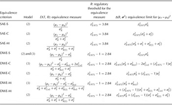
Table 3 summarizes the SAE and DWE criteria for GMO safety evaluation. Due to the reported trivial effects of G × E (Harrigan et al.
Reference Harrigan, Culler, Culler, Breeze, Berman, Halls and Harrison2013; Harrison et al.
Reference Harrison, Howard, Malven, Halls, Culler, Harrigan and Wolfinger2013 and Venkatesh et al.
Reference Venkatesh, Breeze, Liu, Harrigan and Culler2014), the present work considered the simple case of
 $\sigma _{R \times S}^2 = \sigma _{G \times S}^2 = 0$
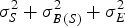
. Figure 2 shows that the three SAE criteria run parallel to the three DWE criteria: SAE-S and DWE-S criteria compare super-distributions. They assess the general class of ‘super-equivalence’, SAE-C and DWE-C criteria compare conditional distributions and hence assess ‘conditional equivalence’, and SAE-M and DWE-M compare marginal distributions and therefore assess ‘marginal equivalence’. The SAE and DWE machineries pave two separate paths from super equivalence to conditional and then to marginal equivalence. One possible way to envision the connection between these two paths is to level their ELs by assigning a common weight to
 $\sigma _R^2 $
, i.e. at ϑ
DWE
= ϑ
SAE
− 1. It turns out that there is a close resemblance between the DWE and SAE criteria: Δ
SAE
−S
(·) = Δ
DWE
−S
(·); Δ
SAE
−C
(·) and Δ
DWE
−C
(·) are both weighted sums of
 $\sigma _R^2 $
and
 $\sigma _E^2 $
; Δ
SAE
−
M
(·) and Δ
DWE
−M
(·) are both weighted sums of
 $\sigma _R^2 $
and
 $\sigma _S^2 + \sigma _{B(S)}^2 + \sigma _E^2 $
. The distinction is in the weights assigned to
 $\sigma _S^2 + \sigma _{B(S)}^2 $
and
 $\sigma _E^2 $
. In contrast to the two SAE criteria, the two DWE criteria allocate lighter weights to
 $\sigma _S^2 + \sigma _{B(S)}^2 $
and
 $\sigma _E^2 $
. This is intuitively sensible since the GMO and reference distributions share the common random components of
 $\sigma _S^2 $
,
 $\sigma _{B(S)}^2 $
while
 $\sigma _R^2 $
is the extra variability in the reference distribution. Setting ϑ
DWE
= ϑ
SAE
− 1 enables the H
1 parameter spaces of the six criteria to be organized according to the inequalities of
 $$\eqalign{{\Delta _{SAE - S}}({\vartheta _{SAE}},{{\bf \sigma} ^2}) &= {\Delta _{DWE - S}}({\vartheta _{DWE}},{{\bf \sigma} ^2})\cr &\quad \lt {\Delta _{DWE - C}}({\vartheta _{DWE}},{{\bf \sigma} ^2}) \cr {\rm} & \quad\lt {\Delta _{SAE - C}}({\vartheta _{SAE}},{{\bf \sigma} ^2})\cr & \quad \;\& \;{\Delta _{DWE - M}}({\vartheta _{DWE}},{{\bf \sigma} ^2})\cr &\quad \lt {\Delta _{SAE - M}}({\vartheta _{SAE}},{{\bf \sigma} ^2})}$$
Summary of equivalence criteria for GMO safety evaluation

It is thus seen that SAE-S/DWE-S represents the most stringent level of equivalence and SAE-M is the most relaxed. Note that there is no definite ordering between SAE-C and DWE-M. Their relationship is controlled by the relative magnitude of
 $\sigma _S^2 + \sigma _{B(S)}^2 $
to
 $\sigma _E^2 $
.
RESULTS
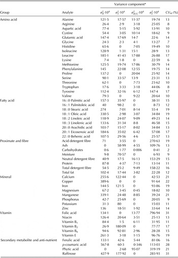
The SAE and DWE criteria were investigated over the range of mixed model parameter values typically encountered in GMO safety evaluation. As far as it is known, the statistical analysis by Van der Voet et al. (Reference Van der Voet, Perry, Amzal and Paoletti2011) is the only public record that documents real-world variance component values of every single compositional endpoint. The exercise in the present work relied on their analysis results (cited in Table 4). It is important to know that the values in Table 4 produce point estimates of ELs and should not be treated as known parameters when testing for equivalence. A valid statistical analysis must account for the uncertainty in estimating (μ T − μ R )2 as well as the EL. Appendix 2 reviews statistical methodologies employed in equivalence testing. The purpose of this exercise was to examine the range of ELs for crop compositional endpoints. The formal statistical analysis of this dataset is not trivial and will be published elsewhere.
Variability of compositional endpoints in a study on GM maize (Van der Voet et al. Reference Van der Voet, Perry, Amzal and Paoletti2011)

CV
M
,
 $\sqrt {\exp (\sigma _R^2 + \sigma _S^2 + \sigma _{B(S)}^2 + \sigma _E^2 ) - 1} $
.
* Variance components in Model (2) are multiplied by 104 for ease in reading.
By Property 1 of the log-normal distribution,
 $\exp (\sqrt {\Delta ( {\cdot} )} )$
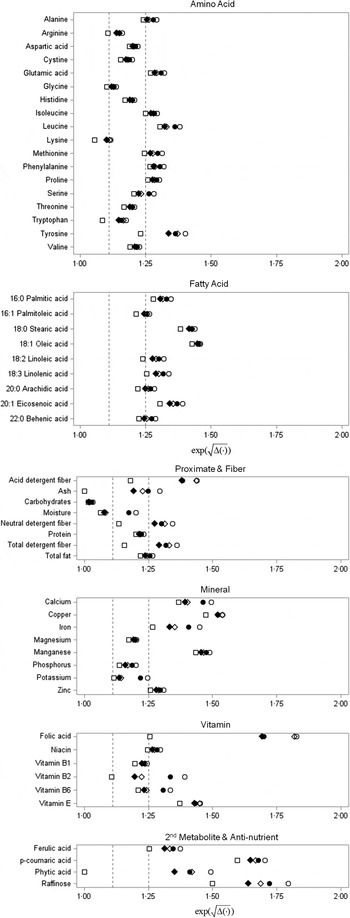
represents the maximum allowable GMO-over-reference ratio of geometric means. Plug the variance component estimates of every analyte in Table 4 into
 $\exp (\sqrt {\Delta ( {\cdot} )} )$
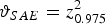
. Figure 3 illustrates the value of
 $\exp (\sqrt {\Delta ( {\cdot} )} )$
for each equivalence criterion (
 ${\vartheta _{SAE}} = z_{0.975}^2 $
;
 ${\vartheta _{DWE}} = z_{0.975}^2 - 1$
). Note that the five distinct criteria numerically reconciled for many analytes. This is due to the fact that
 $\sigma _R^2 $
was often the dominating source of variation. A perhaps comforting surprise was that the maximum allowable ratios of geometric means were not overly broadened in these criteria, as their values were mostly near 1·25. This relates to the fact that many analytes in Table 4 had small to moderate variability (Property 2 of the log-normal distribution indicates that their CVs were near 15%). Three analytes, namely, folic acid, p-coumaric acid and raffinose, had CVs around 30%. If adopting the standard used for evaluating drugs (Midha et al.
Reference Midha, Rawson and Hubbard1997), these analytes fell into the ‘highly variable’ category. As intended, scaling relaxed the maximum allowable ratios in SAE-M to as large as 1·83. The CVs of arginine, glycine, lysine, tryptophan and carbohydrates were 8% or less. Scaling tightened their maximum allowable ratios around or below 1·11. For ash and phytic acid,
 $\sigma _R^2 $
was estimated to be zero while the estimates of
 $\sigma _S^2 $
and
 $\sigma _E^2 $
were considerably large. In these cases, it is unreasonable to pin the maximum allowable ratio at one, as in SAE-S/DWE-S. The maximum allowable ratio of the other four criteria was 1·19~1·29 for ash and 1·35~1·49 for phytic acid, which are more sensible. The visible separation among SAE and DWE criteria also occurred with tyrosine, acid detergent fibre, moisture, neutral detergent fibre, total detergent fibre, iron, potassium, folic acid, vitamin B2 and raffinose. Referring to Table 4, these analytes all had a fair amount of variability with sizable contributions from site, block and/or error term variance components. Ordering of the ELs for the equivalence criteria under Model (2) was confirmed by these analytes as well. Specifically it was observed that when the error term dominated the total variation, as in acid fibre and folic acid, the maximum allowable ratio in the SAE-S/DWE-S criterion was distinctively smaller than in other criteria; when site was the foremost source of variation, as in moisture and vitamin B2, the SAE-M and DWE-M criteria had visibly higher maximum allowable ratios than the others.
Values of
 $\exp (\sqrt {\Delta ( {\cdot} )} )$
, the maximum allowable GMO-over-reference ratio of geometric means, specified by the SAE and DWE criteria. □, SAE-S/DWE-S; ♦, DWE-C; ◊, SAE-C; ●, DWE-M; ○, SAE-M. Dashed line represents the AE maximum allowable ratio of either 1·11 or 1·25. Values of variance components are taken from Table 4.

DISCUSSION
The present paper introduces several equivalence criteria for GMO safety evaluation. The SAE-S and DWE-S criteria compare GMO against references according to their super-distributions. They assess what is called super-equivalence, which could be unreasonably stringent when
 $\sigma _R^2 $
, the variability among reference genotypes, is relatively small. Motivated by the concept of substantial equivalence, the SAE-C, SAE-M, DWE-C and DWE-M criteria define equivalence by taking into account additional sources of natural variation. Note that their ELs are loosened when
 $\sigma _E^2 $
, variance for the error term, is large. Because part of
 $\sigma _E^2 $
comes from variability in sample processing and measurement, Hsuan (Reference Hsuan2000) cautioned that its inclusion in equivalence criteria may reward a sloppy study with an artificially large EL. This concern can be dismissed by the following reasoning. It is important to include plot-to-plot variability as this makes up part of natural variation. Wellek (Reference Wellek2010, Section 10.2.2) speculated that a study with poor quality not only has an excessively high
 $\sigma _E^2 $
but also risks inducing large bias in the estimation of the mean difference; it is thus unlikely for a producer to profit from trying to surreptitiously manipulate these tests. After all, no method of statistical inference is immune to deceptive strategies in data collection. It is the responsibility of the overseeing regulators to guard against fraud. Enforcing compliance with current Good Laboratory Practices is a practical solution to prevent artificial inflation of
 $\sigma _E^2 $
. If values of an endpoint are difficult to quantify analytically, a regulatory authority could require producers to take replicates so as to improve precision. The average of the analytical replicates could then be treated as the response variable in the linear mixed model.
The SAE-C and DWE-C criteria compare GMO with references according to their conditional distributions at the site and block level. They are meant to evaluate conditional equivalence. The SAE-M and DWE-M criteria judge GMO against references on the basis of their marginal distributions across sites and blocks. They are meant to evaluate marginal equivalence which is less stringent than conditional equivalence. The question now becomes what class of equivalence should be used in evaluating GMO safety. Note that forage and grain harvested from different locations is usually bulked for shipment and/or pooled for processing before release to market. From a statistical standpoint, consumers are exposed over time to a blend of the GM product coming from various sites. This diminishes the necessity for demanding equivalence within individual sites. Marginal equivalence across sites and blocks should be sufficient. Empirical evidence consistently demonstrates the trivial effect of G × E in compositional data. Accordingly, there is little biological justification for insisting upon G × E in the safety evaluation of a GM product for food and feed.
Although marginal equivalence is more relevant to GMO safety, the conditional equivalence criteria turn out to be useful. It is observed that producers usually enrol eight to ten sites in their field experiments. Estimating the site-to-site variation,
 $\sigma _S^2 $
, under such a limited sample size is fraught with difficulty and hinders the application of the SAE-M and DWE-M criteria. The situation with
 $\sigma _R^2 $
is quite different, though. Some producers have met the minimum requirement of the EFSA guidance exactly by including only six references per study. Other producers have used as many as 22 references. Kang & Vahl (Reference Kang and Vahl2014) demonstrated that super equivalence could be established with good power when a reasonably large number of references are allocated to sites in an incomplete partially balanced fashion. Upon further validation of their statistical method, conditional equivalence could be established from practical designs. Considering the limited number of sites in current field experiments and the logical dominance of conditional equivalence over marginal equivalence, the SAE-C and DWE-C criteria appear to be more practical and conservative choices than the SAE-M and DWE-M criteria.
A recent symposium on the composition analysis of GM crops proclaimed that ‘composition analysis is meant to look for unintended effects and not to measure natural variation’ (Hoekenga et al.
Reference Hoekenga, Srinivasan, Barry and Bartholomaeus2013). This statement is at odds with the concept of substantial equivalence where a reliable quantification of natural variation is crucial. It comes as a reminder that the experimental design of a study should concentrate on addressing specific scientific questions. If a study is intended to establish marginal equivalence, it must contain enough sites to adequately estimate
 $\sigma _S^2 $
. The position of marginal equivalence at the low end of the hierarchy also provides an incentive for producers to furnish their studies with more sites. This is an immense improvement over the proof-of-difference approach, where producers collecting more data are unfairly burdened with more significant, but spurious, differences to explain away. Testing for equivalence clearly offers the best of both worlds: it grants regulators firm control over consumer risk and encourages producers to conduct scientifically rigorous studies. Another relevant question is whether to enforce Model (3) in order to account for potential G × E effects. Because equivalence criteria entail estimation of variance components from small samples, the degree of complexity in statistical analysis is tremendously amplified as more random effects enter the model (e.g. Öfversten Reference Öfversten1993; Christensen Reference Christensen1996; Burch & Iyer Reference Burch and Iyer1997; Burch Reference Burch2007). This is in contrast to traditional estimation of fixed effects where statistical methods are more forgiving of an overly parameterized model. The extra cost incurred by including trivial random effects may not be worthwhile. Open access to real data will add further clarity. Since there has been no evidence justifying the importance of G × E, Model (2) and its associated equivalence criteria are preferable.
The SAE and DWE criteria under Model (2) pose similar degrees of technical challenge because they both require inference on means as well as variances. The SAE criteria are consistent with the common belief that percentiles of the reference distribution define the ELs for the GMO mean. They also follow the prevailing trend of scaling in drug studies. A DWE criterion is more of a mathematical construct. For in vivo drug studies, it has been labelled as a theoretical solution to a theoretical problem (Patterson Reference Patterson2001; Schall & Endrenyi Reference Schall and Endrenyi2010). Wellek (Reference Wellek2010, p. 312) comments that ‘…statistical BE [bioequivalence] assessment has developed into a field where more mathematically sophisticated solutions exist than problems worth the effort entailed in deriving solutions.’ Yet for assessing GMO equivalence, the underpinning theory for DWE yields a more interpretable formulation. The DWE criteria resonate with the common statistical philosophy of controlling the KL divergence between distributions and are informative even if the data are transformed by monotone functions other than log. Because their ELs assign more weight to the extra variance of the reference distributions, skeptics of GMO may be more willing to accept DWE than SAE. The preference for one type of criteria over the other should be determined through an open dialogue between the ag-biotech industry and regulatory authorities. This process, in part, should be based on an abundance of empirical evidence provided by real-world data.
The present paper intends to challenge traditional thinking and stimulate further research in evaluating GMO safety. Both EFSA (2010) and Van der Voet et al. (Reference Van der Voet, Perry, Amzal and Paoletti2011) assess equivalence via a two-step procedure that replaces the fixed EL in the AE criterion with a data-dependent statistic. Appendix 3 demonstrates the series of issues associated with their approach. Interestingly, similar mistakes have occurred in regulatory applications of bioequivalence and non-inferiority testing (for comments and corrections, see pp. 1866–1867 of Boddy et al. Reference Boddy, Snikeris, Kringle, Wei, Oppermann and Midha1995, pp. 293–294 of Berger & Hsu Reference Berger and Hsu1996; Hung et al. Reference Hung, Wang, Tsong, Lawrence and O'Neil2003). It is hoped that the present work provides a solid statistical framework in support of the concept of substantial equivalence. Further progress in GMO risk assessment is best made through judicious application of statistical rigour and a transparent public debate centred on real-world data. Given an opportunity, statisticians are willing and able to assist regulators in the protection of consumer safety while providing producers scientifically sound yet economical decision rules.
CONCLUSION
Testing for equivalence rather than difference is the appropriate approach for establishing the substantial equivalence of a GM crop to non-GM reference crops with a history of safe use. A necessary first step is to define a reasonable criterion for equivalence. The present work explored criteria generated by the SAE and DWE machineries. Each of the resulting criteria addresses one of three ordered classes of equivalence: super, conditional and marginal. Marginal equivalence adheres most closely to the concept of substantial equivalence. Because conditional equivalence logically implies marginal equivalence and is practically quantifiable from current field studies, the present paper recommends conditional equivalence to assess GMO while encouraging producers to improve their design to enable testing marginal equivalence in the future. Contrary to concerns of the ag-biotech industry, the linear mixed model currently implemented by EFSA was shown to be adequate for assessing equivalence despite its lack of G × E terms.
We gratefully appreciate the comments from the three anonymous referees. Their input was immensely helpful for improving the clarity of the manuscript.
APPENDIX 1: STRATEGIES FOR CONSTRUCTING EQUIVALENCE CRITERIA
Over the past two decades, a number of equivalence criteria have been proposed to assess bioequivalence. Strategies for their construction could be cross-classified according to (i) probability-v. moment-based, (ii) constant-, reference-, v. mixed-scaled, (iii) symmetric v. non-symmetric, (iv) aggregate v. disaggregate. Reviews of these strategies are available from Schall (Reference Schall, Blume and Midha1995a ), Schall & Williams (Reference Schall and Williams1996) and Chen et al. (Reference Chen, Patnaik, Hauck, Schuirmann, Hyslop and Williams2000). Briefly, probability-based criteria are defined in terms of the probability of a random event. For instance, Anderson & Hauck (Reference Anderson and Hauck1990) assessed the conditional equivalence of a drug based on the proportion of individuals in the cross-over design whose test-over-reference ratios of responses fall into a pre-set interval around unity. Meanwhile, Wellek (Reference Wellek1996) and Munk (Reference Munk1996) evaluated bioequivalence based on the proportion of individuals whose test-over-reference ratios are less than unity. Moment-based criteria are constructed directly from the means and variances in the underlying linear mixed model. They were developed in parallel to probability-based criteria. There is a close mathematical connection between probability- and moment-based criteria (Holder & Hsuan Reference Holder and Hsuan1993; Hauck & Anderson Reference Hauck and Anderson1994). Because the dependence on mixed model parameters is less straightforward in the probability-based criteria, FDA (2001) adopts the moment-based criteria for assessing individual and population bioequivalences. The SAE and DWE criteria introduced here are moment-based, too. Constant-scaled criteria compare the difference between test and reference products to a fixed EL. A classic example is the AE criterion. Reference-scaled criteria are created under the ideology that reference variability should be used to standardize the ELs. FDA (2001) recommends the mixed-scaling approach, which utilizes either constant scaling or reference scaling, depending on whether the reference variability is less than an explicit value. This approach circumvents the narrowing effect of scaling for drugs with low variability but a wide therapeutic window. Regarding GMO safety evaluation, the absence of a one-size-fits-all EL for testing AE prevents the application of mixed scaling.
An equivalence criterion with the property of symmetry, i.e. D(T, R) = D(R, T), might be desirable for comparing two chemically equivalent drugs. Dragalin et al. (Reference Dragalin, Fedorov, Patterson and Jones2003) proposed a modified version of KL divergence in order to attain symmetry in bioequivalence criteria. Nonetheless, the pursuit of symmetry triggers controversies in regulatory policies, namely, commutativity and transitivity. Note that GMO and references belong to different genotype groups and therefore should not be handled equally. A statistical test in this regard is expected to prove GMO is equivalent to references, not the other way around. There has also been no indication that an approved GMO will join commercial non-GM crops to serve as a reference for assessing other GMOs. Commutativity and transitivity are then not necessary when choosing equivalence criteria for GMO. The equivalence measures in Hypotheses (5–9) are non-symmetric.
For each of the SAE and DWE criteria discussed here, means and variances are aggregated into a single criterion. Disaggregate criteria, in contrast, evaluate means and variances separately. This idea was systematically implemented by Vourinen & Turunen (Reference Vourinen and Turunen1996) through a stepwise procedure, where the first step establishes bioequivalence between the means of test and reference drugs, the second step establishes bioequivalence in variances, and the final step assures subject-by-drug interaction is relatively small. Many ensembles of disaggregate criteria have been proposed for evaluating bioequivalence (e.g. Chinchilli Reference Chinchilli1996; Vourinen & Turunen Reference Vourinen and Turunen1996; Hauck et al. Reference Hauck, Bois, Hyslop, Gee and Anderson1997; Gould Reference Gould2000; Wellek Reference Wellek2000; Carrasco & Jover Reference Carrasco and Jover2003). These criteria are easy to interpret and omit the trade-off effect inherited by the aggregate bioequivalence criteria, i.e. the mean difference between two drugs could be intractably offset by their difference in variances (Hauck et al. Reference Hauck, Chen, Hyslop, Patnaik, Schuirmann and Williams1996; Midha et al. Reference Midha, Rawson and Hubbard1997). Disaggregate criteria aim at assuring the test product is close to the reference product in each aspect of their distributions, including means, variances and covariance. This requirement is unnecessary for testing GMO because the reference distribution is known beforehand to have more variability than the GMO distribution. Criteria for assessing substantial equivalence are expected to take this additional variability into proper account. As seen from Fig. 3, equivalence criteria introduced here do not overly broaden the ELs for the geometric mean ratio. Concern on the mean-variance tradeoff is then moot. Furthermore, a separate test for interaction is counter-productive given that it is trivial relative to other sources of variation and does not appear to have any practical implications.
Most efforts to date have been spent on creating equivalence criteria for univariate distributions. Munk & Pflüger (Reference Munk and Pflüger1999), Wellek (Reference Wellek2010, Section 8.2), and Chervoneva et al. (Reference Chervoneva, Hyslop and Hauck2007) proposed multivariate analogues of AE, SAE and DWE criteria, respectively. These criteria are tailored to either paired observations or two independent samples. Extension to more complex designs is currently unavailable.
APPENDIX 2: STATISTICAL ANALYSIS METHODS
Various statistical methods have been studied alongside every newly proposed criterion with respect to their feasibility in evaluating equivalence under real-world designs. The traditional nonparametric method discussed by Anderson & Hauck (Reference Anderson and Hauck1990) sacrifices efficiency for robustness and overlooks certain important effects in complex experimental designs. It was quickly supplanted by linear mixed models (Esinhart & Chinchilli Reference Esinhart and Chinchilli1994; Liu & Chow Reference Liu and Chow1997) since the log-normal distribution is deemed appropriate for modelling endpoints in bioequivalence studies. When normality is in doubt or there are unexplainable outliers, nonparametric statistics may still serve as a last resort (a comprehensive review can be found in Chapters 5 and 6 of Wellek Reference Wellek2010; also see Freitag et al. Reference Freitag, Czado and Munk2007). Within the mixed model framework, the asymptotically unbiased restricted maximum likelihood method tends to overestimate mixed model variance components and has been replaced by the method-of-moments approach, which remains unbiased even for small samples (Chen et al. Reference Chen, Patnaik, Hauck, Schuirmann, Hyslop and Williams2000; Endrenyi et al. Reference Endrenyi, Taback and Tothfalusi2000; FDA 2001). The versatile bootstrapping approach was formerly used to estimate the individual and population bioequivalence measures (Schall Reference Schall1995b ; Kimanani Reference Kimanani2000; Shao et al. Reference Shao, Chow and Wang2000; Freitag et al. Reference Freitag, Czado and Munk2007). Also, Chow et al. (Reference Chow, Shao and Wang2003a ) adopted the delta method for assessing population bioequivalence under a collection of cross-over designs. The modified-large-sample method comes as the third method. It was originally developed to generate approximate confidence intervals for linear combinations of variance components (Howe Reference Howe1974; Graybill & Wang Reference Graybill and Wang1980; Ting et al. Reference Ting, Burdick, Graybill, Jeyaratnam and Lu1990). Unlike the bootstrapping approach and the delta method, it is less computationally intensive and has good finite-sample performance (Hyslop et al. Reference Hyslop, Hsuan and Holder2000; Quiroz et al. Reference Quiroz, Ting, Wei and Burdick2002; Chow et al. Reference Chow, Shao and Wang2003b ; Lee et al. Reference Lee, Shao and Chow2004). The modified-large-sample method is currently the preferred approach by FDA (Chen et al. Reference Chen, Patnaik, Hauck, Schuirmann, Hyslop and Williams2000; FDA 2001). Because this method relies on frequentist large-sample theory, simulation studies are needed to verify its feasibility for executing GMO equivalence criteria. A method based on generalized inference offers an alternative approach to estimate functions of mixed model parameters (Tsui & Weerahandi Reference Tsui and Weerahandi1989; Weerahandi Reference Weerahandi1991, Reference Weerahandi1993; Krishnamoorthy & Mathew Reference Krishnamoorthy and Mathew2004; Liao et al. Reference Liao, Lin and Iyer2005; an excellent introduction on generalize inference can be found in Section 1.4 of Krishnamoorthy & Mathew Reference Krishnamoorthy and Mathew2009). It has been used by McNally et al. (Reference McNally, Iyer and Mathew2003) and Chiu et al. (Reference Chiu, Tsai and Liu2010) to execute the individual and population bioequivalence criteria. Recently Kang & Vahl (Reference Kang and Vahl2014) estimated variance components by method of moments under Model (2) and applied the generalized inference approach to execute the SAE-S criterion in testing GMO. The application of generalized inference in executing the other four equivalence criteria awaits further investigation.
Analyzing multivariate data adds more challenge to equivalence tests. EFSA (2010) recommends the ‘informal’ procedure that analyses multiple endpoints one at a time and integrates the results afterwards via graphical representation. Statistically, the task of establishing multivariate equivalence has been tackled by constructing simultaneous equivalence intervals (Brown et al. Reference Brown, Casella and Hwang1995; Berger & Hsu Reference Berger and Hsu1996; Wang et al. Reference Wang, Hwang and Dasgupta1999). It should be born in mind that multivariate equivalence logically demands equivalence at every endpoint. The overall alternative hypothesis for equivalence is an intersection of alternatives for individual endpoints whereas the overall null hypothesis constitutes a union of individual null hypotheses. By the intersection-union principle (Berger Reference Berger1982; Berger & Hsu Reference Berger and Hsu1996), the type I error rate for the overall test cannot be greater than that of an individual test. Quan et al. (Reference Quan, Bolognese and Yuan2001) demonstrated that this type I error rate can fall below the nominal level when correlations among endpoints are low. This is in reverse to the mutivariate difference test, which entails an inflated family-wise type I error rate. From a regulatory standpoint, testing for equivalence deminishes the need to correct for multiplicity and provides good protection against the consumer's risk. This conservativeness increases the burden of proof for producers, though. Adjusting for the deflated type I error in the intersection-union type of hypotheses is mathematically sophisticated and research in this area is limited (Schuirmann Reference Schuirmann1987; Berger & Hsu Reference Berger and Hsu1996; Brown et al. Reference Brown, Hwang and Munk1997).
APPENDIX 3: THE FALLACY OF A DATA-DRIVEN EQUIVALENCE CRITERION
EFSA's decision rule for establishing equivalence is based on a two-step procedure proposed by Van der Voet et al. (Reference Van der Voet, Perry, Amzal and Paoletti2011). Step L of this procedure computes MEP, the margin of error for the two-sided 95% prediction interval of μ
T
− μ
R
− R under Model (2). Step E computes MEP, the margin of error for the 90% confidence interval of μ
T
− μ
R
. Denote the estimate of μ
T
− μ
R
as
 $\hat d$
. The two-step procedure concludes equivalence at the 0.05 significant level when
 $\hat d - MEC \gt - MEP$
and
 $\hat d + MEC \lt MEP$
. Van der Voet et al. (Reference Van der Voet, Perry, Amzal and Paoletti2011) justify this procedure under a completely balanced design by noting that
 $$ \hskip 13pt \eqalign{& MEP = {t_{0.975,d{f_P}}}\sqrt {\hat \sigma _R^2 + \displaystyle{{\hat \sigma _R^2} \over {{n_R}}} + \displaystyle{{\hat \sigma _E^2} \over {{n_S}{n_{B(S)}}}} + \displaystyle{{\hat \sigma _E^2} \over {{n_R}{n_S}{n_{B(S)}}}}}, \cr & MEC = {t_{0.95,d{f_C}}}\sqrt {\displaystyle{{\hat \sigma _R^2} \over {{n_R}}} + \displaystyle{{\hat \sigma _E^2} \over {{n_S}{n_{B(S)}}}} + \displaystyle{{\hat \sigma _E^2} \over {{n_R}{n_S}{n_{B(S)}}}}}.} $$
Constant
 ${t_{0.975,d{f_P}}}$
represents the 97·5th percentile of the t distribution with degrees of freedom df
P
. Terms df
P
and df
C
are computed from their respective sum of weighted variances under the square root. Notation ’^’ indicates the variance component is estimated. The resemblance of MEP
2 to
 $z_{0.975}^2 \sigma _R^2 $
prompted them to test AE with the following data-driven ELs.
 $$ \hskip 64pt \Delta ({t_{0.975,d{\,f_P}}},{{\hat {\bf \sigma}} ^2}) = ME{P^2}$$
Note that
 $ME{P^2} \gt z_{0.975}^2 \hat \sigma _R^2 $
because (1)
 ${t_{0.975,d{f_P}}} \gt {z_{0.975}}$
and (2) the term under the square root of MEP is always greater than
 $\hat \sigma _R^2 $
. Van der Voet et al. (Reference Van der Voet, Perry, Amzal and Paoletti2011) refer to MEP
2 as the ‘outer’ confidence limit of the EL for (μ
T
− μ
R
)2.
Kang & Vahl (Reference Kang and Vahl2014) pointed out a series of issues associated with the two-step procedure. First, using the outer limit of the EL inflates the type I error rate of the testing procedure for a given set of hypotheses. In fact, existing statistical methods for testing equivalence control their type I error rates by plugging in the ‘inner’ confidence limit of the EL (Hyslop et al.
Reference Hyslop, Hsuan and Holder2000; Kang & Vahl Reference Kang and Vahl2014). Second, the two-step procedure does not properly account for variability in estimating
 $\sigma _R^2 $
. The term
 ${{\hat \sigma _R^2} / {{n_R}}} + {{\hat \sigma _E^2} / {({n_S}{n_{B(S)}})}} + {{\hat \sigma _E^2} / {({n_R}{n_S}{n_{B(S)}})}}$
corresponds to the variability in estimating μ
T
− μ
R
. Its double inclusion in the decision rule (i.e. in both MEP and MEC) is logically indefensible. Third, exchanging a z percentile to a t percentile does not adequately address the reference natural variation. Rather, it introduces ambiguity and causes the actual threshold to be higher than the intended level. Kang & Vahl (Reference Kang and Vahl2014) shows that the two-step procedure uses 0·5th and 99·5th percentiles of the reference distribution (assumed by Model (2) to be normal) when n
R
= 6 and 1·8th and 98·2th percentiles when n
R
= 21.
It was argued by Van der Voet et al. (Reference Van der Voet, Perry, Amzal and Paoletti2011) that ‘the null hypothesis value of the test is only established after step L’ and ‘statistical properties of such tests can only be defined conditionally on the outcome of step L’. Contrary to this misconception, statistical procedures involving conditioning have always been studied with respect to their unconditional performance. Theoretical discussion of improper conditioning is provided in Section 10.4 of Lehmann & Romano (Reference Lehmann and Romano2005). Real-world examples can be found in pp. 293–294 of Berger & Hsu (Reference Berger and Hsu1996) as well as Hung et al. (Reference Hung, Wang, Tsong, Lawrence and O'Neil2003). Even though Van der Voet et al. (Reference Van der Voet, Perry, Amzal and Paoletti2011) never explicitly defined the equivalence criterion in terms of parameters in Model (2), they investigated the type I error under Hypotheses (4) with
 $$\Delta (\vartheta, {{\bf \sigma} ^2}) = z_{0.975}^2 \left( {\sigma _R^2 + \displaystyle{{\sigma _R^2} \over {{n_R}}} + \displaystyle{{\sigma _E^2} \over {{n_S}{n_{B(S)}}}} + \displaystyle{{\sigma _E^2} \over {{n_R}{n_S}{n_{B(S)}}}}} \right).$$
However, their simulation study altered the two-step procedure by replacing
 ${t_{0.975,d{f_P}}}$
in MEP with z
0.975 and replacing the estimated variances (
 $\hat \sigma _R^2 $
and
 $\hat \sigma _E^2 $
) by true simulation settings. The reported nominal level of this modified two-step procedure does not justify the statistical properties of their original procedure when applied to data with unknown variances. Kang & Vahl (Reference Kang and Vahl2014) demonstrates that the original two-step procedure carries a type I error rate of 0·353 under the simulation setting of Van der Voet et al. (Reference Van der Voet, Perry, Amzal and Paoletti2011).
Disregarding the statistical properties of the two-step procedure, it may be tempting to retain Formula (A1) as an EL in assessing substantial equivalence. An important reminder to this end is that hypotheses are made with respect to the target population(s) (Chapter 8 of Casella & Berger Reference Casella and Berger2002; Lehmann & Romano Reference Lehmann and Romano2005). In the case of GMO safety evaluation, GMO and reference populations are of interest. Sample sizes have nothing to do with these two populations and should not appear in the hypotheses. A disturbing consequence of Formula (A1) is that producers conducting studies with more references will be punished with a lower EL. Without loss of generality, consider the situation where
 $\sigma _R^2 \gg \sigma _S^2 + \sigma _{B(S)}^2 + \sigma _E^2 $
. Formula (A1) simplifies to
 $\Delta (\vartheta, {{\bf \sigma} ^2}) \approx(1 +{1 / {{n_R}}})$
 $z_{0.975}^2 \sigma _R^2 $
. Suppose there exists a valid equivalence testing procedure for assessing (μ
T
− μ
R
)2 against the EL of
 $(1 + {1 / {{n_R}}})z_{0.975}^2 \sigma _R^2 $
. That is, its type I error rate is no greater than the 0·05 nominal level when
 ${({\mu _T} - {\mu _R})^2} \ge (1 + {1 / {{n_R}}})z_{0.975}^2 \sigma _R^2 $
and its power is greater than 0·05 when
 ${({\mu _T} - {\mu _R})^2} \lt$
 $(1 + {1 / {{n_R}}})z_{0.975}^2 \sigma _R^2 $
. Let two producers, A and B, evaluate the same GM product whose true squared mean deviation from μ
R
is
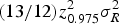 $({{13} / {12}})z_{0.975}^2 \sigma _R^2 $
. Producer A includes six references in his field design (n
R
= 6) and Producer B uses 12 references (n
R
= 12). Because
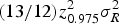 $({{13} / {12}})z_{0.975}^2 \sigma _R^2 $
is at the boundary of the parameter space of H
0 tested by Producer B, he will conclude equivalence with 0·05 probability (nominal type I error rate = 0·05). In contrast, the true squared mean difference is within the parameter space of H
1 tested by Producer A since
 ${{(13} / {12}})z_{0.975}^2 \sigma _R^2 \lt ({7 / 6})z_{0.975}^2 \sigma _R^2 $
. He will conclude equivalence with greater than 0·05 probability (power > 0·05). Producer B with a larger sample size is therefore unfairly penalized by a more stringent EL than the one used by Producer A.
In summary, variability of an estimator should not be folded into the EL. Rather, its impact should be lessened by implementing efficient experimental designs in conjunction with unbiased and powerful testing procedures. The ELs of the SAE-C and SAE-M criteria represent better ways to account for natural variation in the reference population.