Nomenclature
-
 ${V_T}$
-
speed of target
-
${V_{Mi}}$
-
speed of the i-th missile
-
${a_{Mi}}$
-
acceleration of the i-th missile
-
${a_T}$
-
acceleration of target
-
${r_i}$
-
relative distance between the i-th missile and target


Greek Symbol
-
${\lambda _i}$
-
line-of-sight angle of the i-th missile
-
${\lambda _{di}}$
-
desired impact angle of the i-th missile
-
${\gamma _{Mi}}$
-
flight-path angle of the i-th missile
-
${\gamma _T}$
-
flight-path angle of target


1.0 Introduction
With the development of anti-flight vehicle technology, it is difficult to accurately intercept the target with the traditional one-to-one engagement approach [Reference Guo, Hu, Guo and Zhou1]. With the advancement of artificial intelligence, coherence theory and information and communications technology, it is possible to realise real-time information interaction between flight vehicles, further realising the collaboration of multiple flight vehicles in intercepting targets [Reference Jiang, Ge, Xu and Yang2]. Compared to the traditional guidance law, multi-flight vehicle cooperative guidance can effectively improve the flight vehicles survival probability and the destructive effect on the target through communication, information sharing and cooperation among flight vehicles [Reference Han, Pang, Li, Li, Guo, Fan and Li3–Reference Zhang, Yan, Huang, Che, Wang and Lu5].
The traditional cooperative guidance law is to set impact time in advance, and each flight vehicle attacks the target independently according to the given impact time. This technique, termed impact time control guidance (ITCG), functions without the need for information exchange between flight vehicles. The first literature to mention this method can be attributed to Jeon et al. [Reference Jeon, Lee and Tahk6] wherein an ITCG was derived to guide multiple flight vehicles to intercept a stationary target simultaneously. As a further study of Ref. [Reference Jeon, Lee and Tahk6], Jeon et al. [Reference Jeon, Lee and Tahk7] proposed a novel guidance law based on modified proportional navigation guidance (PNG). The concept of their approach was to use a term of time-to-go estimate to achieve an accurate estimate of the impact time against the stationary or moving target. In Ref. [Reference Kim and Shin8], an ITCG law derived from precise nonlinear kinematic equations without time-to-go estimation was presented against a stationary target. Yang et al. [Reference Yang, Xiaoping, Zhou and Fei9] designed a two-phase guidance strategy in which the guidance law developed the heading error to improve the applicability. While the guidance techniques can enable simultaneous intercept targets in certain combat situations, a major limitation is that the timing for each flight vehicle must be predetermined prior to launching multiple flight vehicles [Reference Sinha and Kumar10–Reference Liu, Wang, Rui, Wu, Tang and Gu12].
To address this limitation, due to the advances in multi-agent coherent control theory, cooperative guidance laws based on different communication frameworks have been widely studied. Optimising the damage effect on high-value targets becomes increasingly challenging in the presence of sophisticated close-in weapon systems, making cooperative interception at various impact angles a crucial requirement [Reference Zhang, Guo, Liu, Wang and Hu13]. The authors in Ref. [Reference Chen, Wang, Wang, Shan and Xin14] provided a two-stage cooperative ITCG law using PNG considering field-of-view (FOV) constraint against a stationary target. The thrust control and speed limit are considered in Ref. [Reference Chen, Wang, Shan and Xin15], the proposed approach is designed to realise a salvo attack with the impact angle constrained. As an extension of Ref. [Reference Yang, Xiaoping, Zhou and Fei9], an optimal decentralised three-dimensional (3-D) cooperative guidance law under communication topologies that are dynamically adjusted and directed against a stationary target. In Jianglong et al. [Reference Jianglong, Xiwang, Qingdong, Zhang and Jinhu16], the authors studied the cooperative guidance task of multiple vehicles during the gliding and descending phases of flight, while considering the impact angle and impact time constraints. It is important to highlight that a majority of these studies focus on stationary targets or targets moving at low speeds, without fully accounting for the dynamic interactions among interceptors [Reference He, Wang, Lin, Xiao and Du17]. Additionally, specifying the interception time beforehand is required; however, this does not constitute genuine active collaboration and could constrain the effectiveness.
Finite-time convergence is a crucial requirement for cooperative engagement using the guidance law. Since cooperative guidance involving multiple interceptors must be completed within a finite time frame, during which interception performance metrics are critical, the guidance law must be designed to ensure convergence within this limited period [Reference Zhan, Li and Zhou18, Reference Yang and Yan19]. A novel distributed leaderless guidance law was proposed in Ref. [Reference Dong and Ren20] against manoeuvring targets. The approach was to suggest a disturbance observer to estimate target acceleration. In Ref. [Reference Song, Song and Xu21], a cooperative guidance law with impact angle constraints is presented for the 3-D finite-time terminal guidance problem, where multiple flight vehicles intercept a manoeuvring target. The proposed method is continuous and operates without needing information about the target’s manoeuvres. Although the finite-time cooperative guidance law improves the convergence speed, the efficiency of the finite-time cooperative guidance law is affected by the initial conditions [Reference Mei and Ding22]. Large initial errors lead to long convergence times; if the initial error is sufficiently large, the convergence time could potentially extend to infinity [Reference Huang and Jia23, Reference Ni, Liu, Liu and Liu24].
It is important to note that all the previously mentioned finite-time guidance laws are unable to guarantee a uniformly bounded convergence time. Achieving the desired rapid convergence within a specific time depends on selecting suitable conditions for the flight vehicle. Fixed-time stability, as introduced by Polyakov, expands the concept of finite-time stability by ensuring that the convergence time stays uniformly bounded, regardless of the initial conditions [Reference Polyakov25]. The researchers in Ref. [Reference Li, Ma, Gao and Zang26] investigated a two-dimensional (2-D) fixed-time cooperative guidance law with impact angle constraints based on adaptive super-twisting sliding mode control. In addition, a straightforward fixed-time disturbance observer to estimate and compensate disturbances caused by target acceleration was designed in Ref. [Reference Jing, Zhang, Guo and Cui27]. In Ref. [Reference Dong, Wang, Wang, Zuo and Shan28], the authors presented the development of fixed-time cooperative guidance laws for multiple flight vehicles to intercept a manoeuvring target simultaneously with a desired impact angle. The guidance law proposed in Refs [Reference Chen, Chen, Liu and Cheng29–Reference Yu, Dai, Li, Zou, Ma, Ma and Zhang31] addressed a 3-D fixed time for multiple flight vehicles simultaneously to intercept manoeuvring targets with desired impact angles.
Inspired by the forementioned studies, a novel fast fixed-time cooperative guidance (FFCG) law is proposed in this paper inspired by the studies mentioned above. The key contributions are outlined as follows:
-
1. Compared to studies like Refs [Reference Jeon, Lee and Tahk6–Reference Yang, Xiaoping, Zhou and Fei9], this research introduces a novel method that accounts for communication among interceptors and incorporates both impact angle and time constraints. Using a nonlinear interception model for manoeuvring targets, the guidance law is formulated in two components: one along the LOS direction and the other perpendicular to it. This ensures synchronised arrival times for interceptors and accurate target interception at a predetermined angle within a fixed time. This dual-direction approach is notably distinct from previous single-direction guidance designs, which focused solely on guidance law design in a single direction. This dual-direction design enhances the flexibility and precision of the system.
-
2. Compared with the guidance laws in Refs [Reference Jing, Zhang, Guo and Cui27, Reference He, Fan, Wang and Wang32], the guidance law proposed in this paper designs a disturbance observer with fixed-time convergence to accurately estimate the target LOS acceleration, allowing multiple flight vehicles to intercept the target simultaneously at the desired impact angles. This approach differs significantly from prior research that considered the target’s LOS acceleration as 0.
-
3. The proposed FFCG law allows flight vehicles to cooperatively intercept targets exhibiting various motions (stationary, normal speed and manoeuvring) with different desired impact angles. In addition, this paper also investigates the cooperative guidance task in the communication topology switching state. Finally, the guidance law’s effectiveness and robustness are validated through Monte Carlo simulations and comparative experiments.
-
4. The rest of this paper is structured as follows. Section 2 states the mathematical principles of cooperative guidance of multiple flight vehicles. In Section 3, the proposed fixed-time cooperative guidance law is derived in detail. Section 4 demonstrates the effectiveness and robustness of the proposed law as illustrated through simulations of various engagement scenarios. In Section 5, the study’s conclusions are presented and possible directions for future research are discussed.
2.0 Problem formulation
To simplify the study, this paper employs a kinematic analysis approach based on the following assumptions:
-
1. The interceptors and the target are assumed to have sufficiently fast autopilots, allowing their dynamics to be neglected when designing the guidance strategy.
-
2. The accelerations of both the flight vehicle and the target are always directed perpendicular to their respective constant velocity vectors. The target’s acceleration is unknown but constrained within certain bounds.
Assumption 1 simplifies the development of guidance laws by concentrating only on the dynamics relevant to guidance and eliminating complications from the slower response of the control system. Assumption 2 facilitates modeling and design by emphasising manoeuvres based on direction, while considering uncertainty in the target’s acceleration, albeit within a controllable range. This assumption simplifies the guidance law design by concentrating exclusively on the engagement kinematics, thereby avoiding the complexity introduced by slower autopilot dynamics.
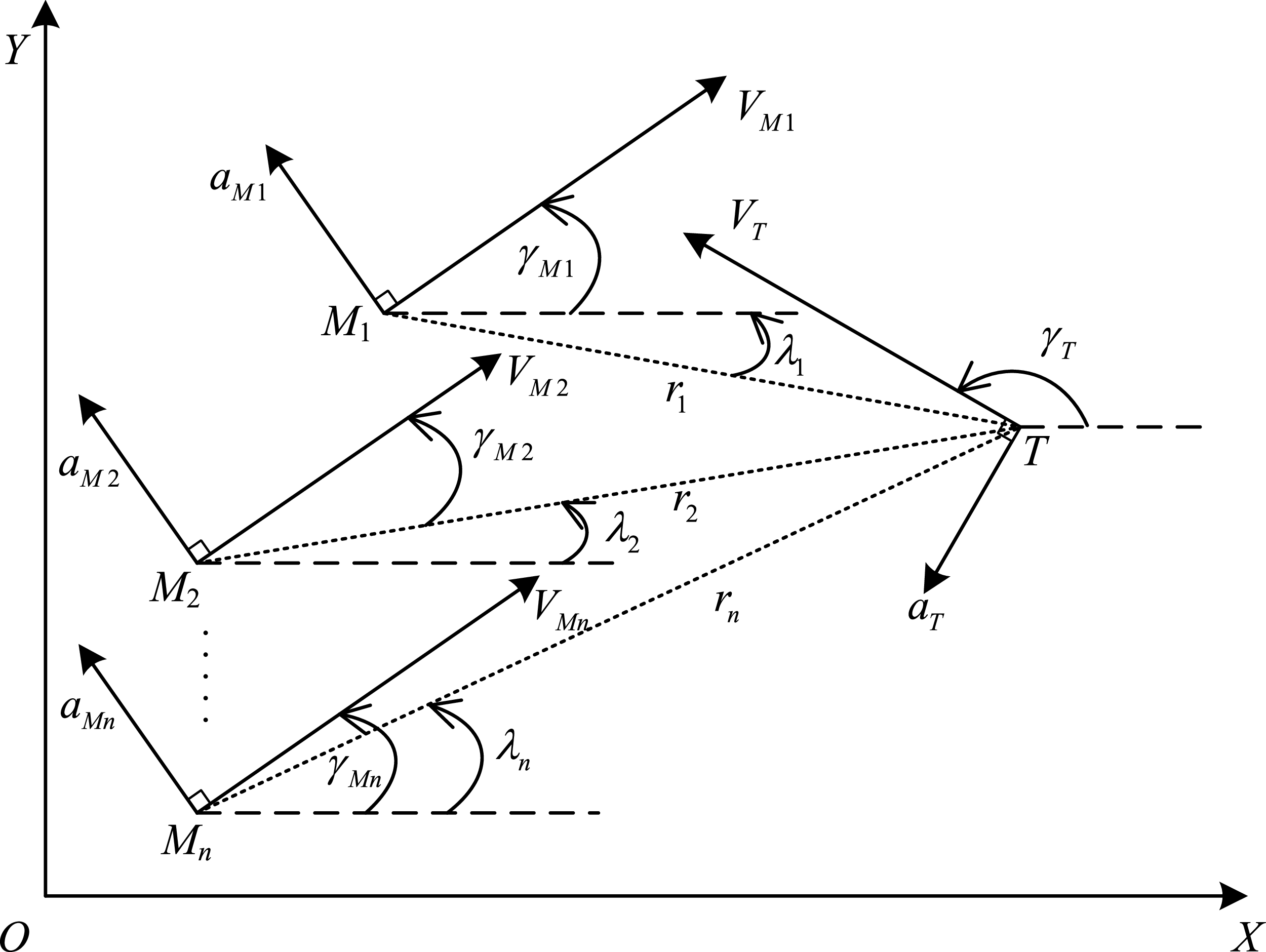
Consider an interception task within the perpendicular plane, utilising a 2-D planar engagement geometry, as illustrated in Fig. 1.
Multiple missiles-target engagement geometry.

Based on Fig. 1, the relative motion equations between the flight vehicles and the target can be obtained as follows:
 \begin{align} {\dot r_i} = {V_T}\cos\!\left( {{\gamma _{Mi}} - {\lambda _i}} \right) - {V_{Mi}}\cos\!\left( {{\gamma _T} - {\lambda _i}} \right)\end{align}
 \begin{align} {r_i}{\dot \lambda _i} = {V_{Mi}}\sin\!\left( {{\gamma _T} - {\lambda _i}} \right) - {V_T}\sin\!\left( {{\gamma _{Mi}} - {\lambda _i}} \right)\end{align}
 \begin{align} {\gamma _{Mi}} = \frac{{{a_{Mi}}}}{{{V_{Mi}}}}\end{align}
 \begin{align} {\gamma _T} = \frac{{{a_T}}}{{{V_T}}}\end{align}
where
 $OXY$
is the inertial reference frame. The flight vehicle and target are denoted by
 ${M_i}$
and
 $T$
, respectively.
 ${r_i}$
represents the distance between the flight vehicle and the target, and the flight vehicle’s LOS angle is denoted by
 ${\lambda _i}$
. The velocities of the flight vehicle and the target are represented by
 ${V_{Mi}}$
and
 ${V_T}$
, respectively.
 ${\gamma _{Mi}}$
and
 ${\gamma _T}$
states the flight path angles of the flight vehicle and the target. The normal accelerations of the flight vehicle and the target are represented by
 ${a_{Mi}}$
and
 ${a_T}$
.
 $i=1,2, \ldots ,n$
,
 $n$
is the number of flight vehicles.
Based on Equations (1) and (2), differentiating
 ${\dot r_i}$
and
 ${\dot \lambda _i}$
with respect to time yields
 \begin{align} {\ddot r_i} &= {r_i}\dot \lambda _i^2 - {u_{ri}} + {w_{ri}} \end{align}
 \begin{align} {\ddot \lambda _i} &= - 2\frac{{{{\dot r}_i}}}{{{r_i}}}{\dot \lambda _i} - \frac{{{u_{qi}}}}{{{r_i}}} + \frac{{{w_{qi}}}}{{{r_i}}}\end{align}
where
 ${u_{ri}}$
and
 ${u_{qi}}$
denote the flight vehicle acceleration along the LOS direction and perpendicular to it, respectively.
 ${w_{ri}}$
and
 ${w_{qi}}$
represent the respective components of the target’s acceleration. The four variables
 ${u_{ri}}$
,
 ${u_{qi}}$
,
 ${w_{ri}}$
and
 ${w_{qi}}$
can be expressed using Equation (7):
 \begin{align}\left\{ \begin{array}{l}{u_{ri}} = - {{\dot V}_{Mi}}\cos\!\left( {{\lambda _i} - {\gamma _{Mi}}} \right) + {a_{Mi}}\sin\!\left( {{\lambda _i} - {\gamma _{Mi}}} \right)\\{u_{qi}} = - {{\dot V}_{Mi}}\sin\!\left( {{\lambda _i} - {\gamma _{Mi}}} \right) + {a_{Mi}}\cos\!\left( {{\lambda _i} - {\gamma _{Mi}}} \right)\\{w_{ri}} = {{\dot V}_T}\cos\!\left( {{\lambda _i} - {\gamma _T}} \right) + {a_T}\sin\!\left( {{\lambda _i} - {\gamma _T}} \right)\\{w_{qi}} = - {{\dot V}_T}\sin\!\left( {{\lambda _i} - {\gamma _T}} \right) + {a_T}\cos\!\left( {{\lambda _i} - {\gamma _T}} \right)\end{array} \right.\end{align}
It can be derived from Equation (7) that
 ${a_{Mi}}$
can be designed from
 ${u_{ri}}$
and
 ${u_{qi}}$
as
 \begin{align}{a_{Mi}} = \sin\!\left( {{\lambda _i} - {\gamma _{Mi}}} \right){u_{ri}} + \cos\!\left( {{\lambda _i} - {\gamma _{Mi}}} \right){u_{qi}}\end{align}
In order to guarantee that several flight vehicles can hit the target at the same time with the specified impact angles, the subsequent nonlinear state equation is formulated.
 \begin{align}\left\{ \begin{array}{l}{x_{1i}} = {r_i}\\{x_{2i}} = {{\dot r}_i}\\{x_{3i}} = {\lambda _i} - {\lambda _{di}}\\{x_{4i}} = {{\dot \lambda }_i}\end{array} \right.\end{align}
The time derivative of Equation (9) is given as
 \begin{align}\left\{ \begin{array}{l}{{\dot x}_{1i}} = {x_{2i}}\\{{\dot x}_{2i}} = {x_{1i}}\,x_{4i}^2 - {u_{ri}} + {d_{ri}}\\{{\dot x}_{3i}} = {x_{4i}}\\[4pt]{{\dot x}_{4i}} = - \dfrac{{2{x_{2i}}}}{{{x_{1i}}}}{x_{4i}} - \dfrac{{{u_{qi}}}}{{{x_{1i}}}} + {d_{qi}}\end{array} \right.\end{align}
where
 ${d_{ri}} = {w_{ri}}$
and
 ${d_{qi}} = {w_{qi}}/{x_{1i}}$
can be considered the interference component caused by the target’s manoeuvre in the direction along and perpendicular to the LOS. Based on Assumption 2,
 $\left| {{d_{ri}}} \right| \le {D_1}$
,
 $\left| {{{\dot d}_{ri}}} \right| \le {D_2}$
,
 $\left| {{d_{qi}}} \right| \le {D_3}$
and
 $\left| {{{\dot d}_{qi}}} \right| \le {D_4}$
, where
 ${D_1}$
,
 ${D_2}$
,
 ${D_3}$
and
 ${D_4}$
are unknown and bounded.
The success of a cooperative interception strategy for multiple flight vehicles depends on ensuring that all vehicles arrive at the target simultaneously with high accuracy and efficiency. This requires satisfying constraints on time convergence and interception precision. Additionally, to enhance target damage effectiveness, impact angle control guidance should be integrated. Consequently, the guidance law is designed with objectives addressing these critical aspects, as shown in Equation (11):
 \begin{align}\left\{ \begin{array}{l}\mathop {\lim }\limits_{t \to {t_{fi}}} {r_i} = 0\\\mathop {\lim }\limits_{t \to {t_{fi}}} {\lambda _i} = {\lambda _{di}}\\\mathop {\lim }\limits_{t \to {t_{fi}}} {{\dot \lambda }_i} = 0\\{t_{f1}} = {t_{f2}} = \cdots = {t_{fi}}\end{array} \right.\end{align}
where
 ${t_{fi}}$
and
 ${\lambda _{di}}$
represent the final interception time and desired impact angle for the flight vehicle
 ${M_i}$
, respectively.
In this paper, a fixed-time cooperative guidance law is developed to enable multiple flight vehicles to simultaneously intercept a manoeuvring target, ensuring that they achieve the desired impact angles. Based on the guidance system in Equation (10), the proposed guidance law designed the control input
 ${u_{ri}}$
in the LOS direction to ensure that
 ${x_{1i}}$
and
 ${x_{2i}}$
reach consensus within a fixed time. Then, the control input
 ${u_{qi}}$
is designed in the normal direction to the LOS to ensure that
 ${x_{3i}}$
and
 ${x_{4i}}$
converge to zero within a fixed time.
3.0 Design of fixed-time convergence cooperative guidance law
In this section, the proposed fixed-time convergence cooperative guidance law is designed through two components along the LOS and perpendicular to it. First, utilising fixed-time consensus theory, a cooperative guidance law is formulated to ensure synchronised timing among multiple flight vehicles. Next, based on fixed-time sliding mode control, the guidance law is designed for the direction perpendicular to the LOS to ensure the impact angle and LOS angular rate converge rapidly within a fixed time.
3.1 Preliminary lemmas
Building on the foundational concepts, several lemmas are now introduced to address finite-time consistent convergence. These lemmas provide the mathematical framework necessary to analyse and design guidance strategies ensuring rapid and precise coordination.
Lemma 1. [Reference Ni, Liu, Chen and Liu33]. Consider a nonlinear system expressed as
 \begin{align}\dot x(t) = f({x(t)}), x(0) = {x_0}\end{align}
where
 $x\!\left( t \right) = {\left[ {{x_1}\left( t \right),{x_2}\left( t \right), \ldots ,{x_n}\left( t \right)} \right]^T} \in {\mathbb{R}^n}$
. When the origin is Lyapunov stable and there exists a settling time
 $T\left( {{x_0}} \right)$
ensuring
 $\mathop {\lim }\limits_{t \to T\left( {{x_0}} \right)} x\!\left( t \right) = 0$
for any
 ${x_0} \in {\mathbb{R}^n}$
, the system demonstrates finite-time stability. Furthermore, if
 $T\left( {{x_0}} \right)$
is uniformly bounded by a constant
 ${T_{\max }}$
, the system achieves fixed-time stability.
Lemma 2. [Reference Zhang, Wei, Jing and Cui34]. For system in Equation (12), assume a Lyapunov function
 $V(x)$
, such that
 $\dot V(x) \le - {\left( {\alpha {V^p}(x) + \beta {V^q}(x)} \right)^k}$
, where
 $\alpha ,\beta ,p,q$
and
 $k$
are positive constants, satisfies
 $\,kp \lt 1$
,
 $\,kq \gt 1$
. The system is fixed-time stable if these conditions are satisfied. The convergence time T is bounded above as
 \begin{align}T \le {T_{\max }} = \frac{1}{{{\alpha ^k}( {1 - kp})}} + \frac{1}{{{\beta ^k}({kq - 1})}}\end{align}
Lemma 3. [Reference Ménard, Moulay and Perruquetti35]. For a disturbed system
 $\dot x = u + d$
with disturbances represented as
 $d$
,
 $\hat d$
is the estimated value of the actual disturbance. According to the following nonlinear disturbance observer,
 $\hat d$
can converge to the actual disturbance
 $d$
within a fixed time.
 \begin{align}\left\{ {\begin{array}{*{20}{l}}{{{\dot z}_1} = {l_3}{l_1}v\left( {x - {z_1},{q_1},{p_1}} \right) + u + {z_2}}\\[3pt]{{{\dot z}_2} = l_3^2{l_2}v\left( {x - {z_1},{q_1},{p_1}} \right)}\\[3pt]{\hat d = {z_2}}\end{array}} \right.\end{align}
where
 ${l_1},{l_2} \gt 0$
,
 ${l_1} \geq 2\sqrt {{l_2}} $
,
 ${l_3} \geq 1$
,
 $0.5 \lt {q_1} \lt 1$
, and
 $1 \lt {p_1} \lt 1.5$
.
 $v\left( \cdot \right)$
is the correction term and satisfies
 \begin{align}v({x,q,p}) = \left\{ {\begin{array}{*{20}{c}}{{{\left| x \right|}^{{q_1}}}{\rm{sign}}(x), \left| x \right| \lt 1}\\{{{\left| x \right|}^{{p_1}}}{\rm{sign}}(x), \left| x \right| \geq 1}\end{array}} \right.\end{align}
The upper bound of the observer is
 \begin{align}T \le \frac{4}{{{l_3}}}\left( {\frac{1}{{1 - {q_1}}} + \frac{1}{{{p_1} - 1}}} \right)\end{align}
Lemma 4. [Reference He, Fan, Wang and Wang32]. Let
 ${x_1},{x_2}, \ldots ,{x_n} \geq 0$
,
 $0 \lt {p_2} \lt 1 \lt {q_2}$
, then
 \begin{align} \sum\limits_{i = 1}^n {x_i^{{p_1}}} &\geq {\left( {\sum\limits_{i = 1}^n {{x_i}} } \right)^{{p_1}}} \end{align}
 \begin{align} \sum\limits_{i = 1}^n {x_i^{{q_2}}} &\geq {n^{1 - {q_2}}}{\left( {\sum\limits_{i = 1}^n {{x_i}} } \right)^{{q_2}}} \end{align}
Lemma 5. [Reference Zuo36]. Consider a scalar system
 \begin{align}\dot y = - {h_1}{\rm{sig}}{{\rm{n}}^{{m_1}}}y - {h_2}{\rm{sig}}{{\rm{n}}^{{m_2}}}y, y\left( 0 \right) = {y_0}\end{align}
where
 ${h_1} \in {\mathbb{R}_ + }$
,
 ${h_2} \in {\mathbb{R}_ + }$
,
 ${m_1} \gt 1$
and
 $0 \lt {m_2} \lt 1$
. Thus, Equation (19) demonstrates fixed-time stability, and the settling time T can be constrained within a specific upper limit.
 \begin{align}T \le \frac{1}{{{h_1}\left( {{m_1} - 1} \right)}} + \frac{1}{{{h_2}\left( {1 - {m_2}} \right)}}\end{align}
For a positive definite function satisfying
 \begin{align}V \le - {a_1}{V^{{b_1}}} - {a_2}{V^{{b_2}}} + \theta \end{align}
where
 ${a_1},{a_2} \gt 0$
,
 $0 \lt {b_1} \lt 1$
and
 ${b_2} \gt 1$
.
 $\theta $
denotes uncertainty that satisfies
 $\left| \theta \right| \le \bar \theta $
, then the positive definite function
 $V$
can converge to
 $V \le {\left( {\bar \theta /\left( {{c_1}{a_1}} \right)} \right)^{1/{b_1}}}$
in fixed-time T, and the upper bound of the fixed-time convergence is
 \begin{align}T \le {T_{\max }} = \frac{{2\bar \theta /{{\left( {{c_2}{a_2}} \right)}^{\frac{{1 - {b_1}}}{{{b_2}}}}}}}{{\phi \left( {1 - {c_1}} \right)}}\end{align}
where
 $\phi = \min \left[ {{a_1}\left( {1 - {b_1}} \right),{a_2}\left( {{b_2} - 1} \right)} \right]$
,
 $0 \lt {c_2} \lt {c_1} \lt 1$
.
3.2 Guidance law design in the LOS direction
Based on the system in Equation (10), the cooperative guidance model is defined as follows
 \begin{align}\left\{ {\begin{array}{*{20}{l}}{{{\dot x}_{1i}} = {x_{2i}}}\\{{{\dot x}_{2i}} = {x_{1i}}x_{4i}^2 - {u_{ri}} + {d_{ri}}}\end{array}} \right.\end{align}
The time-to-go of the flight vehicle
 ${M_i}$
during the cooperative interception process can be estimated using Equation (24), as referenced in Ref. [Reference Zhang, Guo, Liu, Wang and Hu13].
 \begin{align}{t_{goi}} = - \frac{{{r_i}}}{{{{\dot r}_i}}} = - \frac{{{x_{1i}}}}{{{x_{2i}}}}\end{align}
By differentiating Equation (24) with respect to time, the resulting expression can be derived as follows.
 \begin{align}{\dot t_{goi}} = - 1 + \frac{{x_{1i}^2x_{4i}^2}}{{x_{2i}^2}} - \frac{{{x_{1i}}}}{{x_{2i}^2}}{u_{ri}} + \frac{{{x_{1i}}}}{{x_{2i}^2}}{d_{ri}}\end{align}
Based on Equation (25), it is assumed that
 \begin{align}{t_{fi}} = t + {t_{goi}}\end{align}
where
 $t$
is the time elapsed since the flight vehicle was launched.
The time derivative of Equation (26) is given as
 \begin{align}{\dot t_{fi}} = 1 + {\dot t_{goi}} = \frac{{x_{1i}^2x_{4i}^2}}{{x_{2i}^2}} - \frac{{{x_{1i}}}}{{x_{2i}^2}}{u_{ri}} + \frac{{{x_{1i}}}}{{x_{2i}^2}}{d_{ri}}\end{align}
To achieve a simultaneous intercept on the target, the following equation can be obtained.
 \begin{align}{t_{fi}} - {t_{fj}} = {t_{goi}} - {t_{goj}}\end{align}
As shown in Equation (28), it can be observed that the fixed-time uniform convergence of
 ${t_{goi}}$
is equivalent to
 ${t_{fi}}$
.
To establish fixed-time synchronisation of impact time, the following control protocols are proposed.
 \begin{align} {\dot t_{fi}} &= u_i^{nom} \end{align}
 \begin{align} u_i^{nom} &= {\rm{sig}}{{\rm{n}}^{{\beta _1}}}\left\{ {{k_1}{\rm{sig}}{{\rm{n}}^{{\alpha _1}}}\left[ {\sum\limits_{j = 1}^n {{a_{ij}}\left( {{t_{fj}} - {t_{fi}}} \right)} } \right] + {k_2}{\rm{sig}}{{\rm{n}}^{{\alpha _2}}}\left[ {\sum\limits_{j = 1}^n {{a_{ij}}\left( {{t_{fj}} - {t_{fi}}} \right)} } \right]} \right\} \end{align}
where
 ${k_1}$
,
 ${k_2} \gt 0$
,
 ${\alpha _2} \gt {\alpha _1}$
,
 ${\alpha _1}{\beta _1} \lt 1$
and
 ${\alpha _2}{\beta _1} \gt 1$
.
 ${\rm{sig}}{{\rm{n}}^\alpha }(x) = {\left| x \right|^\alpha }{\rm{sign}}(x)$
.
The cooperative guidance law can be obtained as
 \begin{align}{u_{ri}} = {x_{1i}}x_{4i}^2 - \frac{{x_{2i}^2}}{{{x_{1i}}}}u_i^{nom} + \frac{{x_{2i}^2}}{{{x_{1i}}}}{d_{ri}}\end{align}
In order to estimate the target’s manoeuvre in the direction of LOS
 ${d_{ri}}$
in Equation (31) according to Lemma 3, the fixed-time nonlinear interference observer can be depicted as
 \begin{align}\left\{ {\begin{array}{*{20}{l}}{{{\dot z}_{r1i}} = {l_3}{l_1}v\left( {{t_{fi}} - {z_{r1i}},{q_1},{p_1}} \right) + \dfrac{{{x_{1i}}x_{4i}^2}}{{x_{2i}^2}} - \dfrac{{{x_{1i}}}}{{x_{2i}^2}}{u_{ri}} + {z_{r2i}}}\\[5pt]\begin{array}{l}{{\dot z}_{r2i}} = l_3^2{l_2}v\left( {{t_{fi}} - {z_{r1i}},{q_1},{p_1}} \right)\\[3pt]{{\hat d}_{ri}} = {z_{r2i}}\end{array}\end{array}} \right.\end{align}
where
 ${z_{r1i}}$
and
 ${z_{r2i}}$
are estimates of
 ${t_{fi}}$
and
 ${d_{ri}}$
, respectively. The observation errors
 $\left| {{t_{fi}} - {z_{r1i}}} \right|$
and
 $\left| {{d_{ri}} - {z_{r2i}}} \right|$
will converge to zero at a fixed time.
Based on Equation (32), the guidance command in Equation (31) is rewritten as follows
 \begin{align}{u_{ri}} = {x_{1i}}x_{4i}^2 - \frac{{x_{2i}^2}}{{{x_{1i}}}}u_i^{nom} + \frac{{x_{2i}^2}}{{{x_{1i}}}}{z_{r2i}}\end{align}
Theorem 1. In the cooperative guidance system described by Equation (10), when the fixed-time disturbance observer in Equation (32) converges to
 ${z_{r2i}}$
, the cooperative guidance law from Equation (33) collectively ensures that all flight vehicles achieve simultaneous interception of the target within a fixed time.
Proof. Let us consider the Lyapunov candidate function as
 \begin{align}{V_{{r_i}}} = \frac{1}{4}\sum\limits_{i = 1}^n {\sum\limits_{j = 1}^n {{a_{ij}}{{\left( {{t_{fj}} - {t_{fi}}} \right)}^2}} } \end{align}
Substituting Equation (29) into the time derivative of
 ${V_{{r_i}}}$
yields the following equation:
 \begin{align}{{\dot V}_{{r_i}}} &= \sum\limits_{i = 1}^n {\frac{{\partial \dot V(x)}}{{\partial {t_{fi}}}}{{\dot t}_{fi}}} \nonumber\\ &= - \sum\limits_{j = 1}^n {{a_{ij}}\left( {{t_{fj}} - {t_{fi}}} \right)} {\rm{sig}}{{\rm{n}}^{{\beta _1}}}\left\{ {{k_1}{\rm{sig}}{{\rm{n}}^{{\alpha _1}}}\left[ {\sum\limits_{j = 1}^n {{a_{ij}}\left( {{t_{fj}} - {t_{fi}}} \right)} } \right] + {k_2}{\rm{sig}}{{\rm{n}}^{{\alpha _2}}}\left[ {\sum\limits_{j = 1}^n {{a_{ij}}\left( {{t_{fj}} - {t_{fi}}} \right)} } \right]} \right\}\nonumber\\ &= - \left| {\sum\limits_{j = 1}^n {{a_{ij}}\left( {{t_{fj}} - {t_{fi}}} \right)} } \right|{\left| {{k_1}{{\left| {\sum\limits_{j = 1}^n {{a_{ij}}\left( {{t_{fj}} - {t_{fi}}} \right)} } \right|}^{{\alpha _1}}} + {k_2}{{\left| {\sum\limits_{j = 1}^n {{a_{ij}}\left( {{t_{fj}} - {t_{fi}}} \right)} } \right|}^{{\alpha _2}}}} \right|^{{\beta _1}}}\end{align}
According to the Lemma 4, Equation (35) can be represented
 \begin{align}{{\dot V}_{_{{r_i}}}} &\le - {\left| {{k_1}\sum\limits_{i = 1}^n {{{\left| {\sum\limits_{j = 1}^n {{a_{ij}}\left( {{t_{fj}} - {t_{fi}}} \right)} } \right|}^{{\alpha _1} + \frac{1}{{{\beta _1}}}}} + {k_2}{{\left| {\sum\limits_{j = 1}^n {{a_{ij}}\left( {{t_{fj}} - {t_{fi}}} \right)} } \right|}^{{\alpha _2} + \frac{1}{{{\beta _1}}}}}} } \right|^{{\beta _1}}}\nonumber\\ &\le - {\left| {{k_1}{{\left( {\sum\limits_{i = 1}^n {{{\left| {\sum\limits_{j = 1}^n {{a_{ij}}\left( {{t_{fj}} - {t_{fi}}} \right)} } \right|}^2}} } \right)}^{\frac{{{\alpha _1}{\beta _1} + 1}}{{2{\beta _1}}}}} + {k_2}{\alpha _2}^{\frac{{\left( {{\alpha _2} - 2} \right){\beta _1} + 1}}{{2{\beta _1}}}}{{\left( {\sum\limits_{i = 1}^n {{{\left| {\sum\limits_{j = 1}^n {{a_{ij}}\left( {{t_{fj}} - {t_{fi}}} \right)} } \right|}^2}} } \right)}^{\frac{{{\alpha _2}{\beta _1} + 1}}{{2{\beta _1}}}}}} \right|^{{\beta _1}}}\nonumber\\ &\le {\left| {{k_1}{{\left( {2{\lambda _2}\left( {{L_A}} \right)V} \right)}^{\frac{{{\alpha _1}{\beta _1} + 1}}{{2{\beta _1}}}}} + {k_2}{\alpha _2}^{\frac{{\left( {{\alpha _2} - 2} \right){\beta _1} + 1}}{{2{\beta _1}}}}{{\left( {2{\lambda _2}\left( {{L_A}} \right)V} \right)}^{\frac{{{\alpha _2}{\beta _1} + 1}}{{2{\beta _1}}}}}} \right|^{{\beta _1}}}\end{align}
where the value
 $2{\lambda _2}\left( {{L_A}} \right)$
is identified as the second smallest eigenvalue of matrix
 ${L_A}$
.
Based on Lemma 2,
 ${T_1}$
is upper bounded by
 \begin{align}{T_{{r_1}}} \le \frac{{{n^{\frac{{\left( {n - 2} \right){\beta _1} + 1}}{{2{\beta _1}}}}}}}{{{\lambda _2}\left( {{L_A}} \right)}}\left( {\frac{1}{{{k_1}\left( {1 - \dfrac{{{\alpha _1}{\beta _1} + 1}}{2}} \right)}} + \frac{1}{{{k_2}\left( {\dfrac{{{\alpha _2}{\beta _1}}}{2} - 1} \right)}}} \right)\end{align}
Based on Lemma 3, the upper bound of the observer’s convergence time is given by the following expression:
 \begin{align}{T_{{r_2}}} \le \frac{4}{{{l_3}}}\left( {\frac{1}{{1 - {q_1}}} + \frac{1}{{{p_1} - 1}}} \right)\end{align}
Equation (38) confirms that under the guidance command in Equation (33), the variables
 ${t_{fi}}$
will reach fixed-time convergence
 ${T_r} = {T_{{r_1}}} + {T_{{r_2}}}$
. This demonstrates the capability to synchronise
 ${t_{fi}}$
in the direction of LOS, ensuring time consistency through consensus theory. Thus, Theorem 1 is rigorously validated.
3.3 Guidance law design normal to the LOS
The objective of the guidance law in the direction normal to the LOS is to ensure each flight vehicle’s LOS angle converges to the desired value while its angular rate approaches zero. This allows all flight vehicles to intercept the target simultaneously from different angles, achieving an all-around coordinated attack.
From the system in Equation (10), the cooperative guidance model for the normal direction to the LOS is derived as follows
 \begin{align}\left\{ \begin{array}{l}{{\dot x}_{3i}} = {x_{4i}}\\[4pt]{{\dot x}_{4i}} = - \dfrac{{2{x_{2i}}}}{{{x_{1i}}}}{x_{4i}} - \dfrac{{{u_{qi}}}}{{{x_{1i}}}} + {d_{qi}}\end{array} \right.\end{align}
To cooperatively intercept target and the need to converge to the vicinity of the zero domain in a fixed time, the following fixed-time convergence sliding mode variables are developed:
 \begin{align}{s_i} = {x_{4i}} + {\delta _1}{\rm{si}}{{\rm{g}}^{{\sigma _1}}}({x_{3i}}) + {\delta _2}{\rm{si}}{{\rm{g}}^{{\sigma _2}}}({x_{3i}})\end{align}
where
 ${\delta _1},{\delta _2} \gt 0$
,
 $0 \lt {\sigma _1} \lt 1$
and
 ${\sigma _2} \gt 1$
.
By taking the derivative of Equation (40), and substituting Equation (39) into it results in
 \begin{align}{\dot s_i} = - \frac{{2{x_{2i}}}}{{{x_{1i}}}}{x_{4i}} - \frac{{{u_{qi}}}}{{{x_{1i}}}} + {\delta _1}{\sigma _1}{\left| {{x_{3i}}} \right|^{{\sigma _1} - 1}}{\dot x_{3i}} + {\delta _2}{\sigma _2}{\left| {{x_{3i}}} \right|^{{\sigma _2} - 1}}{\dot x_{3i}} + {d_{qi}}\end{align}
Based on Equation (41) and Lemma 5, the guidance law normal to the LOS can be obtained:
 \begin{align}{u_{qi}} = - 2{x_{2i}}\,{x_{4i}} + {\delta _1}{\sigma _1}{\left| {{x_{3i}}} \right|^{{\sigma _1} - 1}}{x_{4i}}{x_{1i}} + {\delta _2}{\sigma _2}{\left| {{x_{3i}}} \right|^{{\sigma _2} - 1}}{x_{4i}}{x_{1i}} + {h_1}{\rm{sig}}{{\rm{n}}^{{m_1}}}{s_i} + {h_2}{\rm{sig}}{{\rm{n}}^{{m_2}}}{s_i} + {x_{1i}}{d_{qi}}\end{align}
Similar to the previous Equation (32), to estimate the disturbance
 ${d_{qi}}$
normal to the LOS in Equation (42). Using Lemma 3, the nonlinear fixed-time disturbance observer, integrated into the cooperative guidance law in the direction perpendicular to the LOS, can be expressed as follows:
 \begin{align}\left\{ {\begin{array}{*{20}{l}}{{{\dot z}_{q1i}} = {l_3}{l_1}v\left( {{x_{4i}} - {z_{q1i}},{q_1},{p_1}} \right) - \dfrac{{2{x_{2i}}{x_{4i}}}}{{{x_{1i}}}} - \dfrac{1}{{{x_{1i}}}}{u_{qi}} + {z_{q2i}}}\\[3pt]\begin{array}{l}{{\dot z}_{q2i}} = l_3^2{l_2}v\left( {{x_{4i}} - {z_{q1i}},{q_1},{p_1}} \right)\\[3pt]{{\hat d}_{qi}} = {z_{q2i}}\end{array}\end{array}} \right.\end{align}
where
 ${z_{q1i}}$
and
 ${z_{q2i}}$
are estimates of
 ${x_{4i}}$
and
 ${d_{qi}}$
. The observation errors
 $\left| {{x_{4i}} - {z_{q1i}}} \right|$
and
 $\left| {{d_{qi}} - {z_{q2i}}} \right|$
will converge to zero at a fixed time.
Using the disturbance observer described in Equation (43), the guidance command from Equation (42) can be reformulated to incorporate the estimated disturbance terms:
 \begin{align}{u_{qi}} = - 2{x_{2i}}{x_{4i}} + {\delta _1}{\sigma _1}{\left| {{x_{3i}}} \right|^{{\sigma _1} - 1}}{x_{4i}}{x_{1i}} + {\delta _2}{\sigma _2}{\left| {{x_{3i}}} \right|^{{\sigma _2} - 1}}{x_{4i}}{x_{1i}} + {h_1}{\rm{sig}}{{\rm{n}}^{{m_1}}}{s_i} + {h_2}{\rm{sig}}{{\rm{n}}^{{m_2}}}{s_i} + {x_{1i}}{z_{q2i}}\end{align}
The proposed approach ensures the guidance system compensates for uncertainties, achieving precise and stable performance within a fixed time.
Theorem 2. For the guidance model Equation (10) in the direction normal to the LOS, the fixed-time nonlinear disturbance observer in Equation (43) ensures convergence within a fixed time. Combined with the sliding mode surface in Equation (40) and the guidance law Equation (44), this approach guarantees that each flight vehicle’s LOS angle reaches the desired value. This coordination enables precise target engagement with desired impact angles.
Proof. Based on Lemma 3, the upper bound of the observer is defined as
 \begin{align}{T_{{q_1}}} \le \frac{4}{{{l_3}}}\left( {\frac{1}{{1 - {q_1}}} + \frac{1}{{{p_1} - 1}}} \right)\end{align}
The Lyapunov candidate is designed as
 \begin{align}{V_{{s_i}}} = \frac{1}{2}s_i^2\end{align}
Based on Assumption 2,
 $\left| {{d_{qi}} - {{\hat d}_{qi}}} \right| \le D$
, where
 $D$
is unknown and bounded. By differentiating Equation (46), the following expression is derived:
 \begin{align}{{\dot V}_{{s_i}}} &= {s_i}{{\dot s}_i}\nonumber\\ & = - \frac{{{\delta _1}}}{{{x_{1i}}}}{\left| {{s_i}} \right|^{{\sigma _1} + 1}} - \frac{{{\delta _2}}}{{{x_{1i}}}}{\left| {{s_i}} \right|^{{\sigma _2} + 1}} + {s_i}{{\tilde d}_{qi}}\nonumber\\ & \le - \frac{{{\delta _1}}}{{{x_{1i}}}}{\left| {{s_i}} \right|^{{\sigma _1} + 1}} - \frac{{{\delta _2}}}{{{x_{1i}}}}{\left| {{s_i}} \right|^{{\sigma _2} + 1}} + \left| {{s_i}} \right|D \end{align}
According to Hölder’s inequality, Equation (47) can be modified as follows:
 \begin{align}{{\dot V}_{{s_i}}} &\le - \frac{{{\delta _1}}}{{{x_{1i}}}}{\left| {{s_i}} \right|^{{\sigma _1} + 1}} - \frac{{{\delta _2}}}{{{x_{1i}}}}{\left| {{s_i}} \right|^{{\sigma _2} + 1}} + \left| {{s_i}} \right|D\nonumber\\ & \le - \frac{{{\delta _1}}}{{{x_{1i}}}}{\left| {{s_i}} \right|^{{\sigma _1} + 1}} - \frac{{{\delta _2}}}{{{x_{1i}}}}{\left| {{s_i}} \right|^{{\sigma _2} + 1}} + \frac{1}{{{\sigma _1} + 1}}{\left| {{s_i}} \right|^{{\sigma _1} + 1}} + \frac{{{\sigma _1}}}{{{\sigma _1} + 1}}D\nonumber\\ & \le - {2^{\frac{{{\sigma _1} + 1}}{2}}}\left( {\frac{{{\delta _1}}}{{{x_{1i}}}} - \frac{1}{{{\sigma _1} + 1}}} \right)V_{{q_1}}^{\frac{{{\sigma _1} + 1}}{2}} - {2^{\frac{{{\sigma _2} + 1}}{2}}}\frac{{{\delta _2}}}{{{x_{1i}}}}V_{{q_1}}^{\frac{{{\sigma _2} + 1}}{2}} + \frac{{{\sigma _1}}}{{{\sigma _1} + 1}}D \end{align}
Based on Lemma 5,
 ${V_{{q_1}}}$
can converge to neighbourhood of domain 0 in a fixed time, and the upper bound
 ${T_{{q_2}}}$
is given as
 \begin{align}{T_{{q_2}}} \le \frac{{2{{\bar \theta }_{{q_2}}}/{{\left( {{c_{{q_{22}}}}{a_{{q_{22}}}}} \right)}^{\frac{{1 - {b_{{q_{21}}}}}}{{{b_{{q_{22}}}}}}}}}}{{{\phi _{{q_2}}}\left( {1 - {c_{{q_{21}}}}} \right)}}\end{align}
where,
 \begin{align*}{a_{{q_{21}}}} &= {2^{\frac{{{\sigma _1} + 1}}{2}}}\left( {\frac{{{\delta _1}}}{{{x_{1i}}}} - \frac{1}{{{\sigma _1} + 1}}} \right)\!, {a_{{q_{22}}}} = {2^{\frac{{{\sigma _2} + 1}}{2}}}\frac{{{\delta _2}}}{{{x_{1i}}}}\nonumber\\ {b_{{q_{21}}}} &= \frac{{{\sigma _1} + 1}}{2}, {b_{{q_{22}}}} = \frac{{{\sigma _2} + 1}}{2}\nonumber\\ {\bar \theta _{{q_2}}} &= \frac{{{\sigma _1}}}{{{\sigma _1} + 1}}D, {\phi _{{q_2}}} = \min [ {{a_{{q_{21}}}}({1 - {b_{{q_{21}}}}}),{a_{{q_{22}}}}( {{b_{{q_{22}}}} - 1} )} ], 0 \lt {c_{{q_{22}}}} \lt {c_{{q_{21}}}} \lt 1.\end{align*}
Based on the above proof it can be obtained by
 \begin{align}{\dot x_{3i}} = - {\delta _1}{\rm{si}}{{\rm{g}}^{{\sigma _1}}}({x_{3i}}) - {\delta _2}{\rm{si}}{{\rm{g}}^{{\sigma _2}}}({x_{3i}})\end{align}
On the basis of Lemma 5, thus, Equation (19) is fixed-time stable and the settling time T can be bounded by
 \begin{align}{T_{{q_3}}} \le \frac{1}{{{\delta _1}\left( {{\sigma _1} - 1} \right)}} + \frac{1}{{{\delta _2}\left( {1 - {\sigma _2}} \right)}}\end{align}
Thus, the guidance law presented in Equation (44) is capable of directing the target along the LOS normal, ensuring that the system converges to a region near the zero domain within a fixed time
 ${T_q}$
, where
 ${T_q} = {T_{{q_1}}} + {T_{{q_2}}} + {T_{{q_3}}}$
.
4.0 Simulation results
In this section, the effectiveness and robustness of the fixed-time cooperative guidance law with impact angle constraints are validated through four sections. In Section 4.1, the performance with different motions of the target based on a fixed communication topology is depicted. Section 4.2 considers the communication topology is dynamic and switching, which proves the effectiveness and generalisability of FFCG law. To demonstrate the robustness of the guidance law developed in this paper, Monte Carlo experiments are shown in Section 4.3. Section 4.4 validates the accuracy and speed of the proposed algorithm through comparative experiments. The experiment considers the case of three flight vehicles simultaneously intercepting the manoeuvring target in the plane with the same guidance law parameters, communication topology and different flight vehicle initial conditions.
The proposed fixed-time cooperative guidance law uniformly addresses various target motion types through the same guidance structure, demonstrating its generality and robustness.
For stationary targets, the disturbance observers remain active but estimate negligible disturbances, ensuring consistent performance without requiring any modification to the guidance law. For constant-velocity moving targets, the observers estimate constant disturbances in the LOS and normal directions, which are effectively compensated in the guidance commands to maintain synchronisation and impact angle accuracy. For manoeuvring targets, the fixed-time observers estimate the unknown time-varying components of target acceleration in real time. Enable the interceptor to maintain the desired impact angle and arrival synchronisation, even when the target’s motion is unpredictable.
This unified approach eliminates the need for mode switching or target motion classification, simplifying implementation while ensuring robust performance across all engagement scenarios. The effectiveness of this design is demonstrated through the simulation results, where the same guidance law successfully intercepts stationary, constant-velocity, and manoeuvring targets with high precision.
The parameters used for the disturbance observer in Equations (32) and (43) are given as
 ${l_1} = 1$
,
 ${l_2} = 2$
,
 ${l_3} = 1$
,
 ${q_1} = 0.8$
and
 ${p_1} = 1.2$
. The observer parameters listed above are selected based on the fixed-time stability conditions established in Lemma 3 and the theoretical framework of Ménard et al. [Reference Ménard, Moulay and Perruquetti35]. Specifically, the gains
 ${l_1}$
,
 ${l_2}$
and
 ${l_3}$
are chosen to ensure the linearised error dynamics are stable, while
 ${q_1}$
and
 ${p_1}$
are tuned to balance convergence speed and noise attenuation. The initial value of the disturbance observer is set as 0. The parameters of the LOS direction in Equation (30) are
 ${\beta _1} = 2$
,
 ${\alpha _1} = 0.4$
,
 ${\alpha _2} = 1.6$
,
 ${k_1} = 1.5$
and
 ${k_1} = 1.5$
. The parameters of LOS normal in Equation (42) are
 ${\delta _1} = 1$
,
 ${\delta _2} = 1$
,
 ${\sigma _1} = 0.9$
,
 ${\sigma _2} = 2$
,
 $\,{m_1} = 0.4$
,
 ${m_2} = 2$
,
 ${h_1} = 250$
and
 ${h_2} = 250$
. To reduce the chatter caused by symbolic function, the
 ${\rm{sign}}(x)$
is replaced by
 ${\rm{tanh}}(\alpha x)$
, where
 $\alpha = 500$
. In real-world scenarios, dynamic actuators have capacity limitations. Therefore, the accelerations that can be exerted are assumed to have an upper limit, which is specified as follows:
 \begin{align} {u_{ri}} &= \left\{ {\begin{array}{*{20}{l}}{{u_{r\max }}{\rm{sign}}\left( {{u_{ri}}} \right)}&\quad{if\left| {{u_{ri}}} \right| \geq {u_{r\max }}}\\{{u_{r\max }}}&\quad{if\left| {{u_{ri}}} \right| \lt {u_{r\max }}}\end{array}} \right.\\[-7pt] \nonumber\end{align}
 \begin{align} {u_{qi}} &= \left\{ {\begin{array}{*{20}{l}}{{u_{q\max }}{\rm{sign}}\left( {{u_{qi}}} \right)}&\quad{if\left| {{u_{qi}}} \right| \geq {u_{q\max }}}\\{{u_{q\max }}}&\quad{if\left| {{u_{qi}}} \right| \lt {u_{q\max }}}\end{array}} \right. \end{align}
where
 ${u_{r\max }} = 30g$
,
 ${u_{q\max }} = 40g$
,
 $g = 9.81{\rm{m/}}{{\rm{s}}^2}$
are the maximum flight vehicle accelerations.
The simulation uses a fixed step size of 0.001 s, and the experiment concludes once the distance between the flight vehicles and the target drops below 0 s.
4.1 Performance with different motions of target
This section validates the proposed FFCG law through numerical simulations targeting various scenarios, including stationary targets, targets with constant velocity and manoeuvring targets. The simulations comprehensively demonstrate the ITG law’s effectiveness across these different motion profiles. The three cases are as follows:
Case 1
 $\,{V_T} = 0 m/s$
Case 2
 $\,{V_T} = 20 m/s,{a_t} = 0$
Case 3
 $\,{V_T} = 50 {\rm{m/s}},{a_t} = 2g\sin\!\left( t \right)$
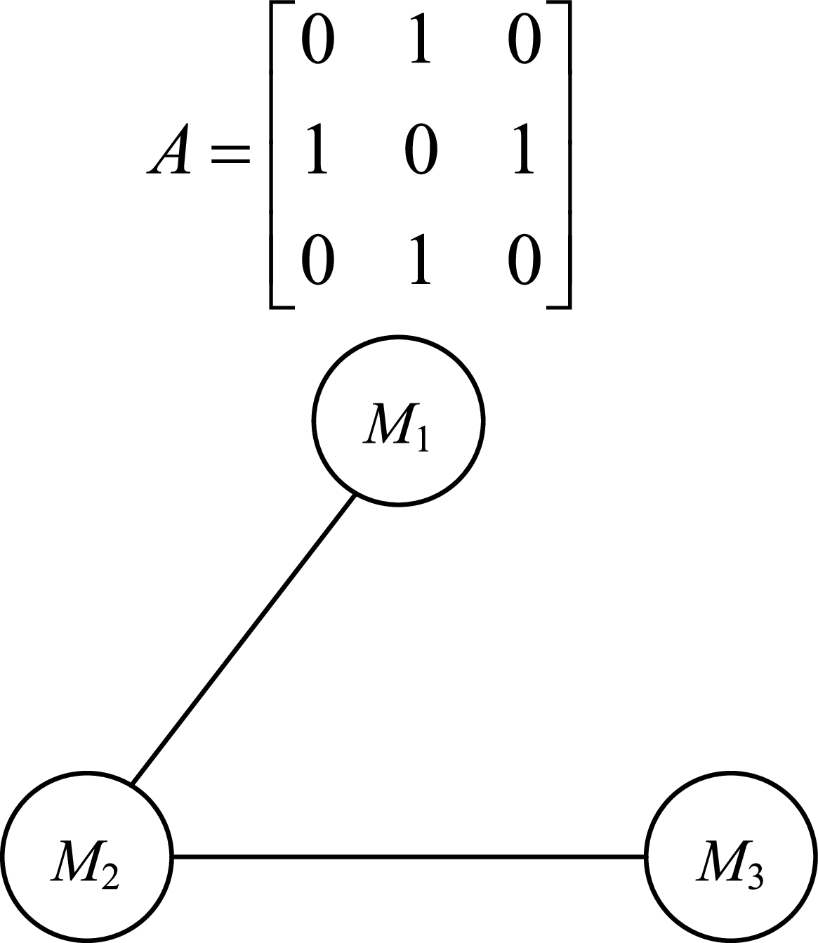
The communication topology among the three flight vehicles remains constant, as illustrated in Fig. 2. This topology is undirected and connected, with its corresponding weight coefficient matrix defined as follows:
 \begin{align}A = \left[ {\begin{array}{*{20}{c}}0&\quad1&\quad0\\[2pt]1&\quad0&\quad1\\[2pt]0&\quad1&\quad0\end{array}} \right]\end{align}
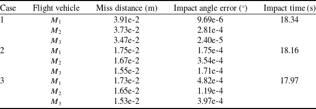
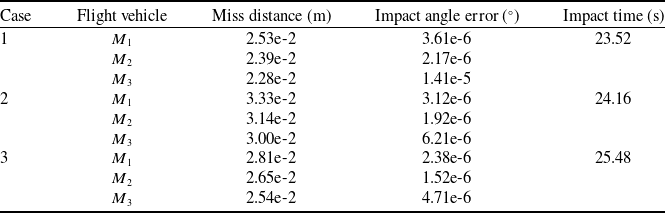
The initial parameters are listed in Table 1. The relative distance, time-to-go, LOS angle, flight vehicle acceleration in and normal to the LOS direction and disturbance observer in Case 3 are depicted in Fig. 3. Furthermore, miss distance, impact angle error and impact time under various simulation cases are listed in Table 2.
Initial parameters for the flight vehicles and target

Miss distance, impact angle error and impact time under various simulations cases

Communication topological structure for three flight vehicles.

Simulation results under Case 3. (a) Relative distance, (b) Time to go, (c) LOS angle, (d) Flight vehicle acceleration in LOS, (e) Flight vehicle acceleration normal to LOS, (f) Disturbance observer.

As shown in Fig. 3(a), the proposed guidance law enables three flight vehicles to intercept a manoeuvring target simultaneously with minimal miss distance. In Fig. 3(b), the time-to-go for all three flight vehicles converged on the same time, five seconds. Figure 3(c) demonstrates that the guidance law in the normal direction to the LOS effectively ensures the convergence of each flight vehicle’s LOS angle to the desired value. Figure 3(d) illustrates that due to the varied initial positions and relative angles of the flight vehicles, the guidance commands in the LOS direction initially show large fluctuations but quickly stabilise, approaching zero over time. As shown in Fig. 3(e), the guidance law normal to the LOS angle is larger in the initial phase, the system needs larger control commands to converge to the sliding mold surface. It can be observed from Fig. 3(f) that the traditional method of treating target perturbations in the direction of the angle of sight as zero does not result in accurate target intercepts. The proposed cooperative guidance law demonstrates strong performance, allowing three flight vehicles to effectively coordinate and intercept a manoeuvring target. This highlights the ability to achieve successful engagement through cooperative strategies.
Further, from the first and second column of Table 2, the proposed guidance law in this paper has excellent guidance accuracy in all cases even when the target motion state is different. With the increase of target manoeuvring capability, the miss distance of all flight vehicles is less than 0.039 m and the error of the desired impact angle is less than 4.82e-4 degrees. Table 2 demonstrates that the cooperative guidance law introduced in this study achieves high precision, with minimal errors in miss distance and desired impact angle. This validates the effectiveness and broad applicability of the FFCG law.
4.2 Performance with switching communication topology
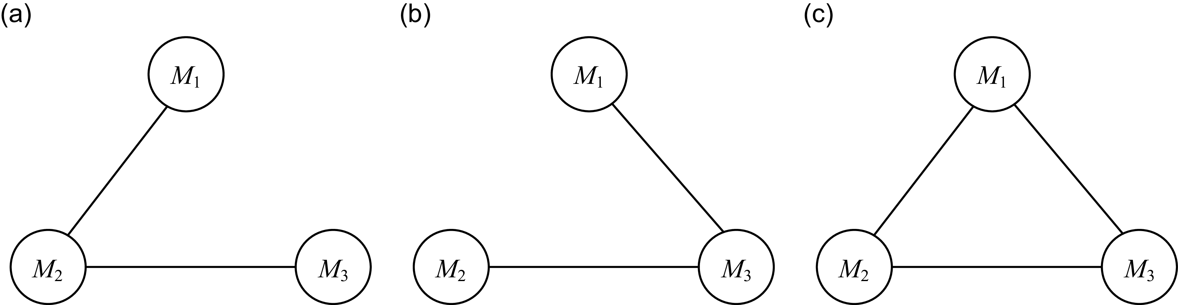
Section 4.1 assumes a fixed communication topology among flight vehicles. The focus now shifts to scenarios where the communication topology is dynamic and subject to switching, impacting the cooperative guidance system’s performance and behaviour. The target motions are based on Section IV-A. Fig. 4 illustrates three types of communication topologies.
The topology transitions are assumed to occur as follows: it switches from topology 1 to 2 at two seconds and further changes to topology 3 at four seconds. This result demonstrates the system’s adaptability to dynamic communication structures during cooperative flight vehicle guidance. The corresponding weight coefficient matrix is
 \begin{align}{A_1} = \left[ {\begin{matrix}0&\quad1&\quad0\\1&\quad0&\quad1\\0&\quad1&\quad0\end{matrix}} \right],{A_2} = \left[ {\begin{matrix}0&\quad0&\quad1\\0&\quad0&\quad1\\1&\quad1&\quad0\end{matrix}} \right],{A_3} = \left[ {\begin{matrix}0&\quad1&\quad1\\1&\quad0&\quad1\\1&\quad1&\quad0\end{matrix}} \right]\end{align}
The initial parameters are different from those in the previous subsection, as listed in Table 3. Like in Section 4-1, three flight vehicles are initialised with distinct starting conditions and desired impact angles to evaluate the cooperative guidance law’s performance. In Case 3, key parameters like relative distance, time-to-go, LOS angle, flight vehicle accelerations along and perpendicular to the LOS direction and disturbance observer outputs are displayed in Fig. 5. Additionally, Table 4 provides a summary of the miss distance, impact angle error and impact time for various simulation scenarios, showcasing the effectiveness and precision under different conditions.
Initial parameters for the flight vehicles and target

Flight vehicles’ various interaction topologies. (a) Topology 1, (b) Topology 2, (c) Topology 3.

Simulation results under Case 3. (a) Relative distance, (b) Time to go, (c) LOS angle, (d) Flight vehicle acceleration in LOS, (e) Flight vehicle acceleration normal to LOS, (f) Disturbance observer.

Miss distance, impact angle error and impact time under various simulations cases

From Fig. 5 and Table 4, all the flight vehicles are able to intercept the target simultaneously at the desired impact angle. Moreover, the proposed approach has superior convergence speed and accuracy under the condition of topology switching. As the target manoeuvrability increases, the time for the flight vehicles to hit the target increases, but the miss distance and impact angle error are within acceptable limits. This demonstrates the system’s adaptability to dynamic communication structures during cooperative flight vehicle guidance.
4.3 Robustness against uncertainties
This subsection verifies the robustness of the proposed approach against measurement noises through a series of Monte Carlo simulations. It aims to test how well the guidance law performs under varying initial conditions and noise levels, ensuring its reliability and effectiveness in practical scenarios. Monte Carlo simulations provide statistical insights by running numerous iterations with randomised inputs, assessing the consistency and resilience of the system under study. The target motions and initial parameters are based on Section 4.1.
Measurement noises in the relative distance
 ${x_{2i}}$
relative distance rate
 ${x_{2i}}$
, LOS angle
 ${x_{3i}}$
and LOS angle rate
 ${x_{4i}}$
are modeled as zero-mean Gaussian distributions. The respective standard deviations are 0.01 m, 0.01 m/s, 0.01 rad and 10e-6 rad/s. These noise assumptions ensure realistic scenarios for testing the guidance law’s robustness under practical conditions.
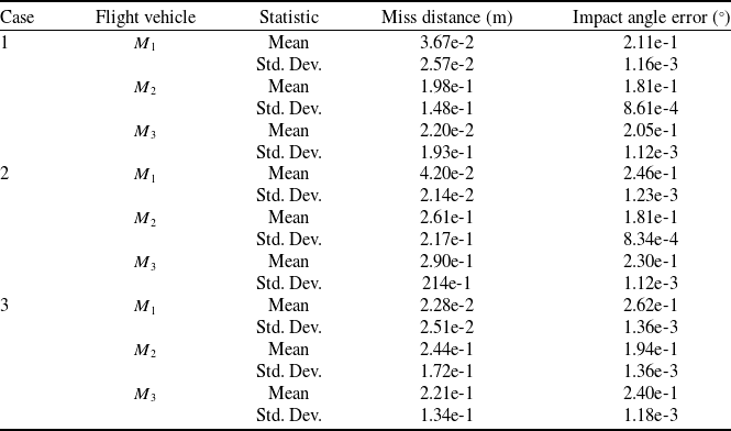
Figure 6 depicts the miss distances, as well as the errors in the desired impact angle, across three scenarios. Table 5 complements this by summarising the mean values and standard deviations for miss distances and impact angle errors, offering a detailed statistical perspective on performance under the tested conditions. The error distance is less than 1 m, and the impact angle error is less than 0.275° in all the experiments, which indicates that the fixed-time cooperative guidance law proposed in this paper still has high accuracy under the conditions of initial error and measurement error. This proves the stability and robustness of the guidance law to meet the practical engineering requirements.
Simulation results under different cases. (a) Miss distance in Case 1, (b) Miss distance in Case 2, (c) Miss distance in Case 3, (d) Impact angle error in Case 1, (e) Impact angle error in Case 2, (f) Impact angle error in Case 3.

Statistical data under various simulations cases

From the data in Table 5, the mean values of miss distance and impact angle error in all experiments are less than 2.90e-1m and 2.46e-1°, respectively, and the standard deviation is less than 2.17e-1m and 1.36e-3°, respectively. These outcomes satisfy the accuracy criteria necessary for executing impact-angle-constrained cooperative attacks in practical scenarios. Monte Carlo simulations further verify that the proposed cooperative guidance law delivers consistent and reliable performance, even in the presence of initial errors and measurement noise.
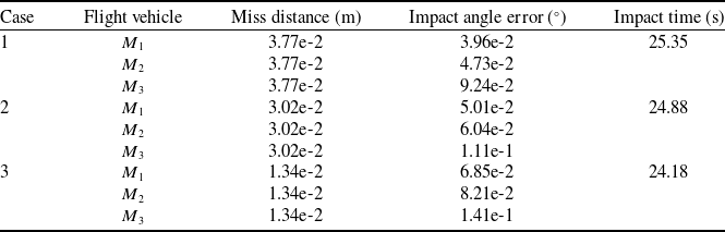
Miss distance, impact angle error and impact time under various simulations cases based on FTCG law

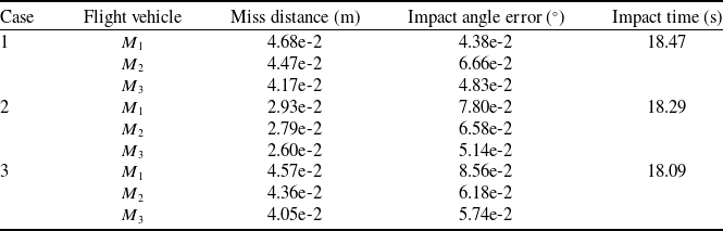
Miss distance, impact angle error and impact time under various simulations cases based on FxTCG law

4.4 Comparison experiment
To better highlight the benefits of the introduced cooperative guidance law, comparative simulation studies are carried out. These simulations contrast the proposed method with a finite-time and fixed-time cooperative guidance law presented in Refs [Reference Jing, Zhang, Guo and Cui27, Reference He, Fan, Wang and Wang32, Reference Lyu, Lyu, Li and Guo37], which is referred as FTCG (finite-time cooperative guidance), FxTCG (fixed-time cooperative guidance), and NFTSMG (nonsingular fast terminal sliding mode guidance) law, respectively.
For the convenience of comparative experiments, the adaptive control law in FxTCG has been removed. The state observer design methodology in NFTSMG is utilised. Identical scenarios and initial conditions are as outlined in Section 4.1. This approach ensures a fair evaluation of performance under consistent settings. The relative distance, time-to-go, LOS angle, flight vehicle accelerations (both in the LOS direction and normal to it) and disturbance observer results for Case 3 are displayed in Figs 7, 8 and 9. Additionally, Table 6, Table 7 and Table 8 present the miss distance, impact angle error and impact time across multiple simulation scenarios, underscoring the guidance law’s effectiveness in diverse conditions.
Simulation results under Case 3 based on FTCG law. (a) Relative distance, (b) Time to go, (c) LOS angle, (d) Flight vehicle acceleration in LOS, (e) Flight vehicle acceleration normal to LOS, (f) Disturbance observer.

Simulation results under Case 3 based on FxTCG law. (a) Relative distance, (b) Time to go, (c) LOS angle, (d) Flight vehicle acceleration in LOS, (e) Flight vehicle acceleration normal to LOS, (f) Disturbance observer.

Simulation results under Case 3 based on NFTSMG law. (a) Relative distance, (b) Time to go, (c) LOS angle, (d) Flight vehicle acceleration in LOS, (e) Flight vehicle acceleration normal to LOS, (f) Disturbance observer.

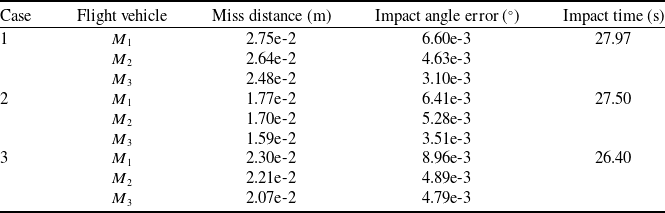
Miss distance, impact angle error and impact time under various simulations cases based on NFTSMG law

Figure 3(a,c), Fig. 7(a,c), Fig. 8(a,c) and Fig. 9(a,c) demonstrate that three cooperative guidance laws effectively enable multiple flight vehicles to intercept a manoeuvring target with the desired impact angle. In terms of time-to-go convergence, the fixed-time consensus control method achieves significantly faster synchronisation compared to the finite-time approach. From Figs 3(d-e), 7(d-e), 8(d-e) and 9(d-e), both guidance laws satisfy the acceleration constraints, but the guidance law command proposed approach is smoother and satisfies the actual command output requirements. FTCG, FxTCG and NFTSMG laws only estimate the disturbance normal to the LOS as depicted in Figs 7(f), 8(f) and 9(f). It can be seen that the perturbation observer with fixed-time convergence converges faster and better.
Quantitative analysis reveals the following key findings. First, in terms of miss distance, the proposed method achieves markedly lower values in Cases 2 and 3 (e.g., M1: 1.75e-2 m and 1.73e-2 m) compared to FTCG (3.02e-2 m and 1.34e-2 m) and FxTCG (2.93e-2 m and 4.57e-2 m), while remaining comparable to or slightly better than NFTSMG (1.59e-2 m to 1.77e-2 m). Second, regarding impact angle error, the proposed law achieves exceptional precision, significantly outperforming the comparison methods. Third, for impact time, the proposed method (17.97 s to 18.34 s) is substantially faster than FTCG (24.18 s to 25.35 s) and NFTSMG (26.40 s to 27.97 s), while matching the speed of FxTCG (18.09 s to 18.47 s).
In conclusion, the proposed cooperative guidance law successfully enables multiple flight vehicles to intercept a manoeuvring target with the desired impact angle within a very short engagement time. Its comprehensive performance, particularly its exceptional precision in impact angle control and competitive miss distance, substantially outperforms the existing FTCG, FxTCG and NFTSMG methods.
5.0 Conclusions
The proposed cooperative guidance law ensures simultaneous engagement of various target motions with desired impact angle, using the multi-intelligence cooperative control theory, disturbance observer and sliding mode control based on the fixed-time convergence. The proposed guidance law has the following advantages:
-
1. Under both fixed and switched topology conditions, the cooperative guidance law has high guidance accuracy with miss distance less than 3.91e-2 m and impact angle error less than 4.82e-4°.
-
2. Since the sliding mode control is characterised by high robustness against perturbation, it can achieve good guidance results even under the disturbance of initial error and measurement error.
-
3. A disturbance observer with fixed-time convergence in and normal to LOS directions is used to control and compensate for the target manoeuvring, which improves guidance accuracy. The proposed guidance law achieves high precision across all target motion types using the same unified structure, demonstrating its generality and practical applicability.
However, there are also the following drawbacks:
-
1. In the initial phase the system requires larger control commands to bring the system closer to the sliding mode surface, diminishing the stability of the system.
-
2. Convergence of guidance law commands normal to the LOS angle is slow and suffers from chatter problems.
In the future, in-depth research will be carried out on the design of cooperative guidance law considering the constraints of flight vehicle dynamics, as well as the analysis of feasible domains of the desired attack direction at the end of each flight vehicle and the quantitative design of the convergence time of the guidance law.
Competing interests
The authors declare that they have no known competing financial interests or personal relationships that could have appeared to influence the work reported in this paper.
Funding statement
This work is supported by the National Natural Science Foundation (NNSF) of China under Grant 62273119.