I. INTRODUCTION
The physics of two-dimensional systems, composed of one or several layers that have thickness of a single atom or a few atoms, is becoming ever more interesting as the realization of such systems with essentially any desirable combination of materials are within grasp of experiment. Reference Geim and Grigorieva1–Reference Xu, Liang, Shi and Chen3 A key issue in such structures is their emergent properties. The environment of an isolated layer is modified by its incorporation into layered assemblies and it is highly desirable to be able to predict the combined system properties from those of isolated parts (layers). There are weak but significant interactions between layers, typically of van der Waals nature, and these need to be taken into account. A big challenge in this direction is that different materials have different in-plane lattice constants, leading to incommensurate structures when they are combined. Even for layers of the same material, it is possible that the layers are not in perfect registry as in the ideal three-dimensional solid, or that one layer is twisted by an arbitrary angle relative to its neighbors, either by accident or by design. Reference Warner, Rümmeli, Gemming, Büchner, Andrew and Briggs4–Reference Brihuega, Mallet, González-Herrero, Trambly de Laissardière, Ugeda, Magaud, Gómez-Rodríguez, Ynduráin and Veuillen8 These issues make the modeling of two-dimensional layered structures crucial for the design and fabrication of materials with desirable properties imperative. Reference Coh, Tan, Louie and Cohen9,Reference Koshino10 Previous theoretical studies have modeled incommensurate twisted bilayers under various approximations such as the tight-binding virtual crystal approximation by Ghader et al., Reference Ghader, Szczȩśniak and Khater11 generalized long-wavelength theory by Pal et al., Reference Pal, Carter and Kindermann12 and also by approximating the incommensurate phases to the nearest commensurate ones. Reference Cao and Li13 Notably, work by Bokdam et al. Reference Bokdam, Amlaki, Brocks and Kelly14 implements a many-body first-principles calculation for commensurate layers where the interlayer potential for incommensurate twisted bilayers is interpolated, and utilizes it to solve a tight-binding Hamiltonian for incommensurate rotations. Since only a few studies have focused on the theoretical aspects of incommensurate systems, a more detailed and robust model needs to be developed.
In the present work, we introduce a simple framework for the study of the electronic structure of layered assemblies based on perturbation theory. Assuming a single-particle picture, we calculate the band structure of commensurate and twisted bilayers of graphene (Gr) and hexagonal boron nitride (h-BN), and of a Gr/h-BN heterostructure, using the wavefunctions and corresponding energy levels of isolated single layers as calculated using density functional theory (DFT) methods. Reference Hohenberg and Kohn15 We find that for relatively large twist in the twisted assemblies, the perturbation of electronic states near the Fermi level is negligible and we also demonstrate how the band structure of a Gr/h-BN heterostructure can be calculated using independent electronic structure calculations of the Gr/Gr and h-BN/h-BN bilayers.
II. METHOD
We first introduce a general theoretical framework for the description of weakly coupled two-dimensional layers of finite dimensions. Consider a system of two single layers initially separated by such distance that the interlayer interaction is negligible. Within the single-particle picture of DFT, the Hamiltonian for each, essentially isolated, layer gives rise to the single-particle (Kohn–Sham) equations Reference Kohn and Sham16 :
 $$\left[ {\hat T\left( {\bf{r}} \right) + V_i^{{\rm{ion}}}\left( {\bf{r}} \right) + {V^{\rm{H}}}\left[ {{\rho _i}} \right]\left( {\bf{r}} \right) + {V^{{\rm{XC}}}}\left[ {{\rho _i}} \right]\left( {\bf{r}} \right)} \right]\psi _i^{\left( {{n_i}} \right)}\left( {\bf{r}} \right) <$$><$$>= \varepsilon _i^{\left( {{n_i}} \right)}\psi _i^{\left( {{n_i}} \right)}\left( {\bf{r}} \right),\quad i = 1,2\quad ,$$
where ρ
i
(r) is the ground-state electron density for the layer characterized by the index i, V
ion[ρ
i
](r) is the external potential due to the presence of the ions of the i-th layer, V
H[ρ
i
](r) is the Hartree (Coulomb) potential generated by ρ
i
, and V
XC[ρ
i
](r) is the exchange-correlation potential. The eigenvalues
 $\varepsilon _i^{\left( {{n_i}} \right)}$
and the eigenstates
 $\psi _i^{\left( {{n_i}} \right)}\left( {\bf{r}} \right)$
are labeled by the index n
i
. We define the total Kohn–Sham potential of the i-th layer as:
 $$V_i^{{\rm{tot}}}\left[ {{\rho _i}} \right]\left( {\bf{r}} \right) = V_i^{{\rm{ion}}}\left( {\bf{r}} \right) + {V^{\rm{H}}}\left[ {{\rho _i}} \right]\left( {\bf{r}} \right) <$$><$$>+ {V^{{\rm{XC}}}}\left[ {{\rho _i}} \right]\left( {\bf{r}} \right),\quad i = 1,2\quad .$$
Bringing the two layers close together to form a weakly coupled combined system leads to the single-particle equations:
 $$\left[ {\hat T\left( {\bf{r}} \right) + V_{12}^{{\rm{ion}}}\left( {\bf{r}} \right) + {V^{\rm{H}}}\left[ \rho \right]\left( {\bf{r}} \right) + {V^{{\rm{XC}}}}\left[ \rho \right]\left( {\bf{r}} \right)} \right]{\psi ^{\left( n \right)}}\left( {\bf{r}} \right) <$$><$$>= {\varepsilon ^{\left( n \right)}}{\psi ^{\left( n \right)}}\left( {\bf{r}} \right)\quad ,$$
where
 $V_{12}^{{\rm{ion}}}\left( {\bf{r}} \right) = V_1^{{\rm{ion}}}\left( {\bf{r}} \right) + V_2^{{\rm{ion}}}\left( {\bf{r}} \right)$
, and where ρ(r) is the ground-state electron density of the whole system. For the combined system, the total Kohn–Sham potential is:
 $$V_{12}^{{\rm{tot}}}\left[ \rho \right]\left( {\bf{r}} \right) = V_{12}^{{\rm{ion}}}\left( {\bf{r}} \right) + {V^{\rm{H}}}\left[ \rho \right]\left( {\bf{r}} \right) + {V^{{\rm{XC}}}}\left[ \rho \right]\left( {\bf{r}} \right)\quad .$$
Equations (1)–(4) provide a formally exact basis for calculating the electronic structure of the combined system using previously obtained solutions for its parts in isolation. We can rewrite the single-particle Hamiltonian operator for the combined system as:
 $${\cal H} = \left[ {\hat T\left( {\bf{r}} \right) + V_1^{{\rm{tot}}}\left[ {{\rho _1}} \right]\left( {\bf{r}} \right) + V_2^{{\rm{tot}}}\left[ {{\rho _2}} \right]\left( {\bf{r}} \right) + {V^{\rm{H}}}\left[ {\Delta \rho } \right]\left( {\bf{r}} \right) <$$><$$>+ \Delta {V^{{\rm{XC}}}}\left[ {\rho ,{\rho _1},{\rho _2}} \right]\left( {\bf{r}} \right)} \right]\quad ,$$
where we have introduced the quantities
 $$\Delta \rho \left( {\bf{r}} \right): = \rho \left( {\bf{r}} \right) - {\rho _1}\left( {\bf{r}} \right) - {\rho _2}\left( {\bf{r}} \right)\quad ,$$
 $$\Delta {V^{{\rm{XC}}}}\left[ {\rho ,{\rho _1},{\rho _2}} \right]\left( {\bf{r}} \right): = {V^{{\rm{XC}}}}\left[ \rho \right]\left( {\bf{r}} \right) - {V^{{\rm{XC}}}}\left[ {{\rho _1}} \right]\left( {\bf{r}} \right) <$$><$$>- {V^{{\rm{XC}}}}\left[ {{\rho _2}} \right]\left( {\bf{r}} \right)\quad .$$
These two quantities depend on the density of the combined system and of each of the individual systems. Notice that due to the interaction, however weak, between the two layers, Δρ(r) ≠ 0. We write the sum of the terms that depend on these quantities as:
 $$\Delta {V_{12}}\left[ {\rho ,{\rho _1},{\rho _2}} \right]\left( {\bf{r}} \right) = {V^{\rm{H}}}\left[ {\Delta \rho } \right]\left( {\bf{r}} \right) + \Delta {V^{{\rm{XC}}}}\left[ {\rho ,{\rho _1},{\rho _2}} \right]\left( {\bf{r}} \right)\quad ,$$
or, equivalently:
 $$\Delta {V_{12}}\left[ {\rho ,{\rho _1},{\rho _2}} \right]\left( {\bf{r}} \right) = V_{12}^{{\rm{tot}}}\left[ \rho \right]\left( {\bf{r}} \right) - V_1^{{\rm{tot}}}\left[ {{\rho _1}} \right]\left( {\bf{r}} \right) <$$><$$>- V_2^{{\rm{tot}}}\left[ {{\rho _2}} \right]\left( {\bf{r}} \right)\quad .$$
The problem is then reduced to finding a satisfactory approximation for the term ΔV 12 defined by Eq. (6), which contains the density ρ(r) of the combined system and it is unknown a priori. The strategy will be to define successive orders of approximation of this term.
In the limit where the interaction between the two layers is very weak,
 $$\Delta \rho \left( {\bf{r}} \right) \approx 0,\quad <$$><$$>\Delta {V^{{\rm{XC}}}}\left[ {\rho ,{\rho _1},{\rho _2}} \right] \approx 0 \Rightarrow \Delta {V_{12}}\left[ {\rho ,{\rho _1},{\rho _2}} \right]\left( {\bf{r}} \right) \approx 0\quad ,$$
which is a reasonable approximation in this case because the weak (van der Waals) interaction of the layers implies that there is very little overlap between the two electron densities corresponding to the isolated layers, even when they are combined into one system. This is the zeroth-order approximation for ΔV 12. In this approximation, it follows from Eq. (6) that before bringing the two single layers close together, the perturbing potential for layer 1 is equal to the total potential of layer 2 and vice versa.
To obtain a first-order approximation, ΔV 12 is calculated using Eq. (6) for a particular finite or periodic configuration of the combined system (we address below what this configuration could be). Once calculated, the same potential can be used for other configurations, that involve relative rotations or displacements of the layers. For infinite periodic or incommensurate layers, the use of ΔV 12 involves an additional practical approximation, namely the potential is taken to depend only on the z coordinate (perpendicular to the plane of the layers) and its dependence on the in-plane (x,y) coordinates is averaged out. This is reasonable because the most important effects of the perturbing potential due to layer 1 on layer 2 will be in the neighborhood of layer 2, where the in-plane modulation of the potential of layer 1 is already weak, and vice versa. Therefore the potential can be approximated by the first term of the in-plane Fourier expansion, which is constant, that is, invariant under rotation or translation and corresponds to its average in-plane value. Note that the relevance of this approximation can be checked numerically. We do not however average the potentials V 1 and V 2. We can then use this expression to calculate the potentials involved in the computation of the perturbation of the Hamiltonian, and with these obtain the solutions of the combined system. In a complementary fashion with tight-binding methods, Reference Ribeiro and Peres17–Reference Fang, Kuate Defo, Shirodkar, Lieu, Tritsaris and Kaxiras19 the scheme outlined above can be applied to any situation and its accuracy will depend on the approximation for ΔV 12.
Within an approximation for the potential ΔV 12, our goal is to compute efficiently the eigenstates of the coupled Hamiltonian defined by Eq. (5) by means of a perturbation approach. We will assume that it is always possible to numerically solve for the states of each isolated layer, that is, Eq. (1) is computationally tractable for i = 1, 2. We want to use these solutions for the states of the isolated layers to obtain a solution for the combined system consisting of two layers, which in general can have incommensurate lattices. The eigenvalue problem for the combined system is:
 $${\cal H}{\psi ^{\left( n \right)}}\left( {\bf{r}} \right) = {\varepsilon ^{\left( n \right)}}{\psi ^{\left( n \right)}}\left( {\bf{r}} \right)\quad ,$$
We look for approximate eigenvectors
 $\psi _N^{\left( n \right)}$
in the linear space spanned by N well-chosen eigenvectors of each isolated layer (modal synthesis), that is,
 $${V_N} = {\rm{Span}}\left\{ {\psi _1^{\left( {{n_1}} \right)},\psi _2^{\left( {{n_2}} \right)}|1\le {n_i} \le N} \right\}\quad ,$$
and we use as a basis for V
N
the set of eigenvectors
 $\left\{ {\psi _1^{\left( 1 \right)}, \ldots ,\psi _1^{\left( N \right)},\psi _2^{\left( 1 \right)}, \ldots ,\psi _2^{\left( N \right)}} \right\}$
such that:
 $$\left( {\hat T\left( {\bf{r}} \right) + V_i^{{\rm{tot}}}\left[ {{\rho _i}} \right]\left( {\bf{r}} \right)} \right)\psi _i^{\left( {{n_i}} \right)}\left( {\bf{r}} \right) = \varepsilon _i^{\left( {{n_i}} \right)}\psi _i^{\left( {{n_i}} \right)}\left( {\bf{r}} \right)\quad {\rm{and}}\quad <$$><$$>\left\langle {\psi _1^{\left( k \right)}|\psi _1^{\left( l \right)}} \right\rangle = \left\langle {\psi _2^{\left( k \right)}|\psi _2^{\left( l \right)}} \right\rangle = {\delta _{kl}}\quad .$$
We now expand
 $\psi _N^{\left( n \right)}$
as
 $$\psi _N^{\left( n \right)} = \\sum\limits_{m = 1}^N c_{1,N}^{\left( {n,m} \right)}\psi _1^{\left( m \right)} + c_{2,N}^{\left( {n,m} \right)}\psi _2^{\left( m \right)}\quad ,$$
and we define the associated vector of coefficients
 $$C_N^{\left( n \right)} = \left( {c_{1,N}^{\left( {n,1} \right)}, \ldots ,c_{1,N}^{\left( {n,N} \right)},c_{2,N}^{\left( {n,1} \right)}, \ldots ,c_{2,N}^{\left( {n,N} \right)}} \right)\quad .$$
The problem expressed by Eq. (7) discretized in the space V N becomes the generalized eigenvalue problem:
 $${{\cal H}_N}C_N^{\left( n \right)} = \varepsilon _N^{\left( n \right)}{S_N}C_N^{\left( n \right)}\quad ,$$
Here
 ${{\cal H}_N}$
and S
N
are two matrices, respectively the discretized Hamiltonian and the overlap matrix. We have, due to the orthonormality condition,
 $${S_N} = \left[ {\matrix{ I & {{S_{12}}} \cr {{{\left( {{S_{12}}} \right)}^† }} & I \cr} } \right]\quad ,$$
where
 $${\left( {{S_{12}}} \right)_{ij}} = \left\langle {\psi _1^{\left( i \right)}|\psi _2^{\left( j \right)}} \right\rangle \quad .$$
Next, the discretized Hamiltonian is given in block form by
 $${{\cal H}_N} = \left[ {\matrix{ {{{\cal H}_{1,N}} + {P_{1,N}}\left( {V_2^{{\rm{tot}}} + \Delta {V_{12}}} \right){P_{1,N}}} & {\Delta {{\cal H}_{12}}} \cr {{{\left( {\Delta {{\cal H}_{12}}} \right)}^† }} & {{{\cal H}_{2,N}} + {P_{2,N}}\left( {V_1^{{\rm{tot}}} + \Delta {V_{12}}} \right){P_{2,N}}} \cr} } \right]\quad ,$$
where
 ${{\cal H}_{1,N}}$
and
 ${{\cal H}_{2,N}}$
are diagonal matrices, P
1,N
and P
2,N
are projectors, respectively. in the bases
 $\left\{ {\psi _1^{\left( 1 \right)}, \ldots ,\psi _1^{\left( N \right)}} \right\}$
and
 $\left\{ {\psi _2^{\left( 1 \right)}, \ldots ,\psi _2^{\left( N \right)}} \right\}$
, and
 $$\eqalign{ {\left( {\Delta {{\cal H}_{12}}} \right)_{ij}} & = \left\langle {\psi _1^{\left( i \right)}|{\cal H}|\psi _2^{\left( j \right)}} \right\rangle \cr & = {1 \over 2}\left( {\varepsilon _1^{\left( i \right)} + \varepsilon _2^{\left( j \right)}} \right)\left\langle {\psi _1^{\left( i \right)}|\psi _2^{\left( j \right)}} \right\rangle <$$><$$>+ \left\langle {\psi _1^{\left( i \right)}|{1 \over 2}\left( {V_1^{{\rm{tot}}} + V_2^{{\rm{tot}}}} \right) + \Delta {V_{12}}|\psi _2^{\left( j \right)}} \right\rangle \quad . \cr}$$
The entries of the matrices
 ${{\cal H}_N}$
and S
N
only contain quantities from the isolated systems, namely the eigenvalues and eigenfunctions
 $\varepsilon _1^{\left( {{n_1}} \right)},|\psi _1^{\left( {{n_1}} \right)}\rangle ,\varepsilon _2^{\left( {{n_2}} \right)},|\psi _2^{\left( {{n_2}} \right)}\rangle$
, and the potentials V
1, V
2 as well as ΔV
12 defined in Eq. (6). To reduce computational burden, the wavefunctions of the combined system can also be constructed in a linear space spanned by sets of near degenerate eigenstates with the minimum difference in energy between these sets being larger than a certain cut-off value, which effectively transforms the problem described by Eq. (10) into a collection of smaller problems.
To summarize, we have introduced an exact formalism for describing the electronic structure of combined systems of finite two-dimensional structures and we discussed approximations for enabling efficient calculations of the involved potentials, and of the solutions for the combined system from solution of its parts through perturbation theory. In what follows we will present illustrations of how the method is applied in periodic cells consisting of two layers of the same material or two different materials, and we discuss on extensions that can approximate incommensurate structures. For all calculations, the DFT potentials, eigenfunctions and eigenvalues are obtained with the GPAW code, Reference Enkovaara, Rostgaard, Mortensen, Chen, Dulak, Ferrighi, Gavnholt, Glinsvad, Haikola, Hansen, Kristoffersen, Kuisma, Larsen, Lehtovaara, Ljungberg, Lopez-Acevedo, Moses, Ojanen, Olsen, Petzold, Romero, Stausholm-Møller, Strange, Tritsaris, Vanin, Walter, Hammer, Häkkinen, Madsen, Nieminen, Nørskov, Puska, Rantala, Schiøtz, Thygesen and Jacobsen20 an implementation of the projector-augmented wave (PAW) method within the frozen core approximation. Reference Blöchl21 The PAW setup for C (B, N) accounts for 4 (3, 5) valence electrons and 2 electrons in the frozen core (GPAW atomic setup release 9672). In the interest of reducing the complexity of the involved calculations, we elected to use the local density approximation for the description of exchange and correlation in the electronic system and a double-ζ plus polarization basis set to represent the Kohn–Sham orbitals. Weak dispersion forces are not captured in this approach, which nevertheless often results in satisfactory (albeit fortuitous) description of the structural characteristics of layered structures. Reference Tritsaris, Malone and Kaxiras22 During structural optimization, the layers are always kept planar on the assumption that the weak interaction does not result in structural relaxation. Within the PAW formalism, use of all-electron wavefunctions instead of their auxiliary (soft) counterparts does not result in significant improvement of the description of the calculated band structures, and for this reason only the PAW pseudowavefunctions and potentials are used here without loss of generality. Core electron states are also neglected as they do not contribute to bonding.
III. PERIODIC SYSTEMS
To illustrate the application of the method, we first consider the case of periodic bilayer systems for which the band structure can be calculated using Bloch's theorem. We calculate the band structure of a commensurate system consisting of two graphene layers in the ideal AB-stacking configuration using the experimental value of 2.47 Å for the in-plane lattice constant. The distance between the two graphene layers is calculated to be 3.35 Å, in agreement with previous theoretical and experimental work.
Reference Lebedeva, Knizhnik, Popov, Lozovik and Potapkin23,Reference Lin, Xu, Hakro, Hasan, Hao, Zhang and Chen24
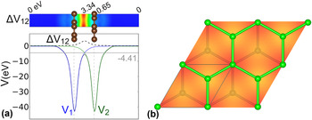
Figure 1 shows the structural configuration of the graphene bilayer, and the potentials (black line) of the combined system and of the separate layers,
 $V_1^{{\rm{tot}}}$
and
 $V_2^{{\rm{tot}}}$
. The potentials V
1 and V
2 are shown averaged in the lateral dimensions (along the planes). The potential ΔV
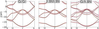
12 is calculated from Eq. (6) to be a positive quantity that is maximized at the midpoint of the distance between the two layers and varies little within the (x,y) plane, which justifies the approximation of in-plane averaging. The calculated band structure is shown in Fig. 2. The solid lines in this plot represent the Kohn–Sham eigenvalues obtained by a DFT calculation, while the red dots indicate the eigenvalues calculated using the perturbation approach outlined above with a cut-off energy that results in a single
 ${{\cal H}_N}$
matrix. As a comparison, the dashed lines indicate the eigenvalues of the isolated layers, which are clearly different than those of the combined system, especially around the center of the Brillouin Zone (Γ-point) for certain bands.
(a) Potentials for the AB-stacked graphene bilayer (black line) and separate layers, V 1 (blue) and V 2 (green), and the potential difference ΔV 12 (black dashed line), shown averaged along the lateral dimensions. The solid gray line marks the Fermi level at −4.41 eV. (b) Potential at the midpoint of the distance between the two graphene layers [same color scheme as on the (a)]. The unit cell is shown repeated twice in the lateral dimensions.

Band structure of the graphene and h-BN bilayers, and of a strained Gr/h-BN heterostructure, in AB-stacked configuration: solid lines are the direct calculation of Kohn–Sham eigenvalues and red dots are the results of the perturbation approach. Green and blue dashed lines indicate the eigenvalues corresponding to isolated layers. The Fermi level is defined as the zero of the energy scale (middle of the band gap for h-BN).

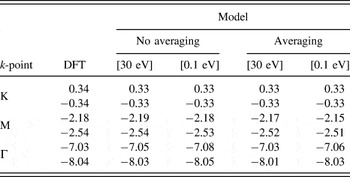
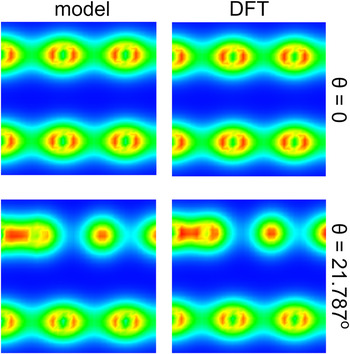
To give a more quantitative comparison, we show in Table I the actual values of π bands at high-symmetry points of the Brillouin Zone, obtained from the perturbation approach model and from direct DFT calculations. The differences in general are very small, regardless of the choice of cut-off energy or of the approximation for the potential ΔV 12 (averaged on the (x,y) plane or not). Figure 3 shows electron densities on a plane that slices through the bilayer for the ideal and twisted graphene, obtained from the perturbation theory model and from direct DFT calculations: the two sets of electron densities are again in excellent agreement. These comparisons demonstrate the high accuracy of our approach.
Comparison between energies obtained from direct DFT calculations and model calculations for AB-stacked bilayer graphene with and without averaging of the potential ΔV 12, and cut-off energy of 30 eV and 0.1 eV, of the π bands at selected high-symmetry k-points. Positive and negative energy values indicate conduction and valence bands, respectively.

Comparison of electron densities, shown on planes that slice through the structure, for the ideal (top row, θ = 0°) and twisted graphene bilayer (twist angle θ = 21.787° in a 7 × 7 configuration, bottom row), calculated with perturbation theory (left column), and directly with DFT (right column).

In Fig. 2, we show a second application of the method, namely the band structure of h-BN. We have considered the AB stacking of the h-BN layers with B on top of the B site. The experimental value of 2.5 Å was used for the in-plane lattice constant and the bilayer was calculated with an optimized value of 3.57 Å for the distance between the two h-BN sheets, in good agreement with previous reports [3.60 Å (Ref. Reference Ribeiro and Peres17)]. As in the case of graphene, there is a very close correspondence between the perturbation approach and the direct DFT calculation. The splitting of the bands around the Γ-point is pronounced, and is successfully captured by our method.
When the lattice constants of different materials are close enough to form a commensurate bilayer, the method described here can be directly applied to obtain the properties of the combined system using a perturbative approach of the isolated systems. As a case in point, we show in Fig. 2 the band structure of a Gr/h-BN bilayer (AB stacking with B on top of C), which satisfies the condition of small strain and is described with remarkable accuracy by our model. The generalized eigenvalue problem is solved using quantities only from independent Gr/Gr and h-BN/h-BN systems in which the interlayer distance is equal to this of the ideal Gr/h-BN system, after stretching the in-plane lattice of the latter by 1% to match that of graphene. The two layers are separated by a distance of 3.13 Å in the calculated minimum-energy configuration although parameters from experiment may also be used. This estimate of interplanar spacing is in reasonable agreement with earlier reported values of 3.22 Å (Ref. Reference Lin, Xu, Hakro, Hasan, Hao, Zhang and Chen24) and 3.2 Å. Reference Fan, Zhao, Wang, Zhang and Zhang25 In this case, the potential ΔV 12 for the heterostructure is approximated by taking the mean value of the respective potentials of the independent bilayer systems, averaged along the lateral dimensions.
IV. PERIODIC APPROXIMATIONS OF INCOMMENSURATE BILAYERS
When two layers with different in-plane lattice constants are placed on top of each other, since they are not strongly bonded to enforce the atoms of layer 2 to be directly above those of layer 1, the resulting combined system can be incommensurate, that is, there will not be a common set of in-plane lattice constants. This is different from the epitaxial growth of three-dimensional structures, in which case the lattice mismatch leads to strain which can be relieved by defects such as dislocations. A different way to form incommensurate layers is to create a stacking of two layers of the same material, in which case the in-plane lattice periodicities are the same, but layer 2 is rotated with respect to layer 1 by an amount that leads to incommensurate in-plane lattices, or lattices that require a very large unit cell to maintain the same in-plane periodicity of both layers. We discuss how our method can be applied to these situations next.
For two different materials, if the in-plane lattice constants of the two layers, denoted by a (1), a (2), have a ratio of:
 $$\lambda = {{{a^{\left( 1 \right)}}} \over {{a^{\left( 2 \right)}}}}:{\rm{irrational}}\;{\rm{number}}\quad {\rm{,}}$$
this can be approximated by rational numbers as:
 $$\lambda \approx {{{m_i}} \over {{n_i}}},\;\left( {{m_i},{n_i}} \right):{\rm{integers}},\;i = 1,2, \ldots \quad ,$$
where the larger the values of (m
i
,n
i
), the closer to the true value of λ we can get. Using this approximation, we can construct supercells for which we can perform periodic cell calculations by taking the supercell lattice constant
 $a_i^{{\rm{sc}}}$
to be
 $$a_i^{{\rm{sc}}} = {n_i}{a^{\left( 1 \right)}} = {m_i}{a^{\left( 2 \right)}}\quad .$$
For example, for the Gr/MoS2 pair: a (1) = 2.46 Å, a (2) = 3.16 Å, so we can have:
 $$\lambda = {{2.46} \over {3.16}} = 0.778481… \approx {4 \over 5}\left( {{\rm{off}}\;{\rm{by}} + 2.8\% } \right) <$$><$$>\approx {{10} \over {13}}\left( {{\rm{off}}\;{\rm{by}} - 1.2\% } \right), \ldots \quad .$$
Actual calculations must also take into account the strain induced by this choice of supercells by minimizing the elastic energy of the system which gives:
 $$a_{i,{\rm{min}}}^{{\rm{sc}}} = {{n_i^2{B_1}{a^{\left( 1 \right)}} + m_i^2{B_2}{a^{\left( 2 \right)}}} \over {{n_i}{B_1} + {m_i}{B_2}}}\quad ,$$
where B 1, B 2 are the two-dimensional bulk moduli, assuming that there is no interaction between the layers, and using the quadratic form of the energy near the minimum for the individual systems in the elastic regime.
In the case where the two layers have the same lattice constants, we can check the accuracy of the formalism developed by creating a supercell that allows for nontrivial rotations between the two layers, capturing some of the effects of the incommensurate stacking. By nontrivial rotations we refer to those which do not lead to identical arrangements of the layers. We will use, as examples, bilayers of graphene and of h-BN, for which the in-plane crystal is the honeycomb lattice. For these lattices, rotations by π/3 or its multiples are trivial rotations, because of the point group symmetry of the lattice. We take the supercell vector
 ${\vec a^{{\rm{sc}}}}$
that produces a periodic arrangement for the combined system at a nontrivial rotation of layer 2 with respect to layer 1 to be given by
 $${\vec a^{{\rm{sc}}}} = p{\vec a_1} + q{\vec a_2},\;{a^{sc}} = |{\vec a^{sc}}| = n|{\vec a_1}| = n|{\vec a_2}|\quad ,$$
where we have assumed that the supercell vectors are of equal length, as in the original lattices, with
 ${\vec a_1}$
,
 ${\vec a_2}$
the two independent lattice vectors of one layer. This leads to the Diophantine equation: p
2 + q
2 + p·q = n
2 which can be solved for the lowest values of the (p, q) pairs to give the supercells of size n and rotation angles, θ
1, θ
2, obtained from the expressions:
 $$\cos \left( {{\theta _1}} \right) = {{p + 2q} \over {2n}},\;\cos \left( {{\theta _2}} \right) = {{2p + q} \over {2n}}\quad .$$
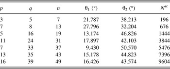
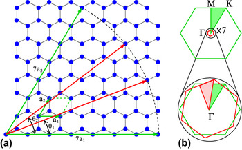
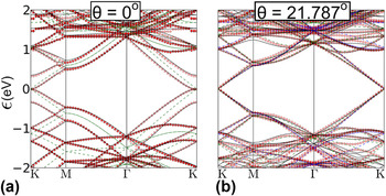
In Table II, we give the solutions (p, q) for the lowest seven values of n and corresponding rotation angles, as well as the total number of atoms in the two-layer honeycomb lattice system. Figure 4 shows an example of the original and rotated lattice vectors for p = 3, q = 5, n = 7. Note that in this case the reciprocal space q-points relevant to the solution belong to the Brillouin Zone of the superlattice which is a folding of the Brillouin Zone of the original single-layer lattice. For the case shown in Fig. 4, it is feasible to perform DFT calculations for the full system consisting of 196 atoms, so that we can directly compare the results of the perturbation model to direct calculations. This comparison is shown in Fig. 5. The potential ΔV
12 is the same as the one used for the ideal (1 × 1) unit cell shown in Fig. 2, averaged in the lateral dimensions, and the cut-off energy is 1 eV. The band structure path is calculated assuming that layer 2 is rotated with respect to layer 1 by an angle θ. In this case, the eigenfunctions
 $\psi _2^{\left( {{n_2}} \right)}$
, are first repeated in space and subsequently are transformed using a (two-dimensional) rotation matrix, while their phases are adjusted according to Bloch's theorem. The perturbation approach gives the splitting of the bands from the two isolated layers, which would otherwise be degenerate (the green dashed lines in Fig. 5). It is interesting that the rotation by θ1 makes the two layers seem almost as completely independent, since in this case, there is essentially no splitting of the bands, especially near the Fermi level (K-point). This has important implications about how the combined incommensurate system will behave, with all the physics essentially captured by the folding of the bands in the new reduced Brillouin Zone, as shown in Fig. 4.
The pairs p and q that satisfy the Diophantine equation and the nontrivial angles of rotation, θ1, θ2, of layer 2 with respect to layer 1. The last column contains the total number of atoms N sc in the two-layer graphene supercell.

(a) Structure of single-layer graphene (with blue circles representing atomic positions) in the (7 × 7) supercell, indicated by green arrows, and the rotated vectors of equal magnitude with nontrivial orientation p = 3, q = 5, n = 7 in the Diophantine equation, in red arrows. The two possible rotation angles, θ1, θ2 are indicated. The primitive lattice constants a 1, a 2 are shown as the small green arrows. (b) Brillouin Zone of the ideal hexagonal lattice [green lines in (a)] and the rotated and folded Zone for the (7 × 7) supercell. The irreducible triangle Γ–K–M is shown shaded in each case.

Band structure of graphene in the (7 × 7) configuration: black solid lines are the direct calculation of Kohn–Sham eigenvalues and red dots are the results of the perturbation approach. Blue and green dashed lines are the eigenvalues corresponding to isolated layers. (a) Ideal stacking. (b) Stacking with relative rotation by θ1 = 21.787°.

V. CONCLUSION
We have introduced a simple framework for the study of the electronic structure of weakly coupled, atom-thick structures of any composition or relative orientation. As demonstrated, our approach enables efficient calculations of electronic structure properties of commensurate and incommensurate layered assemblies based on perturbation theory within the single-particle picture using full-scale DFT calculations. Moreover, obtaining ΔV 12 in a self-consistent manner will enable perturbation calculations using full scale-calculation of only the unit cells of the isolated single-layers. In this way, finer features of the electron density can be captured in twisted assemblies without the need for averaging of the potential. A detailed analysis of this approach is the subject of ongoing work. We stress that our method can be applied to any stacking sequence and any interlayer separation, as long as the layers, commensurate or not, do not strongly interact with each other; this was the case for the heterostructure of graphene and h-BN (Fig. 2), for which the potential ΔV 12 can be approximated by taking the mean value of the respective potentials of independent bilayer systems, averaged along the lateral direction. This is possible because of the weak interaction between the layers and enables calculations of large and complicated multilayer assemblies. Our approach can also be readily extended to the study of excited-state processes at the interfaces in such layered materials, such as charge-carrier motion. Reference Tritsaris, Vinichenko, Kolesov, Friend and Kaxiras26,Reference Kolesov, Vinichenko, Tritsaris, Friend and Kaxiras27 These capabilities of the method open the path for fast computational screening of layered assemblies for targeted design of advanced materials.
ACKNOWLEDGMENTS
This work was supported in part by ARO MURI Award W911NF-14-1-0247. Mitchell Luskin was also supported in part by the Radcliffe Institute for Advanced Study at Harvard University. Calculations were performed on the Extreme Science and Engineering Discovery Environment (XSEDE), which is supported by National Science Foundation Grant No. ACI-1053575.