Implications
Pig carcass composition and cut composition are determinant parameters in the optimization of the production chain. The knowledge of these characteristics with the minimum error in live pigs during growth would be useful in breeding and nutritional programmes to improve the overall economic performance of pig carcasses and to ensure an optimized production to obtain the desired product according to producers and industry demands. This paper shows the feasibility of computed tomography for this purpose and the errors of prediction obtained according to different statistical approaches.
Introduction
Pig growth and body composition are essential components of pig profitability. Weight and composition of gain change in pigs during the growing and finishing periods is determined mainly by the genetic potential and supply of nutrients (Kolstad et al., Reference Kolstad, Jopson and Vangen1996; Kouba et al., Reference Kouba, Bonneau and Noblet1999; Lambe et al., Reference Lambe, Wood, McLean, Walling, Whitney, Jagger, Fullarton, Bayntun and Bünger2013). Knowledge of changes in tissue composition at whole-carcass and primal-cut levels would allow the optimization of slaughter, satisfy niche market demands, and improve the economic efficiency of pork production systems. This information is required as the economic value of pig carcasses is related to the composition of primal cuts rather than the composition of the whole carcass (Marcoux et al., Reference Marcoux, Pomar, Faucitano and Brodeur2007).
Serial slaughtering has traditionally been used to study the body composition of pigs during growth (Fisher et al., Reference Fisher, Green, Whittemore, Wood and Schofield2003; Landgraf et al., Reference Landgraf, Susenbeth, Knap, Looft, Plastow, Kalm and Roehe2006). However, another method used X-ray computed tomography (CT), a non-destructive and non-invasive technique that measures the density of the tissues and allows the body composition of animals to be estimated easily (Kolstad and Vangen, Reference Kolstad, Jopson and Vangen1996; Barchia et al., Reference Barchia, Arthur, Giles and Eamens2010; Lambe et al., Reference Lambe, Wood, McLean, Walling, Whitney, Jagger, Fullarton, Bayntun and Bünger2013); thus, serial slaughtering may no longer be required. Nevertheless, serial slaughtering is still needed to establish the relationship between CT data (i.e. total lean volume) and cutting (joints separation) and dissection (separation of the different tissues of the joints) data and to obtain prediction equations for the weight and composition of main cuts. Several studies have demonstrated that CT is an excellent tool for estimating carcass tissue composition in either pig carcasses (Judas et al., Reference Judas, Höreth and Dobrowolski2006; Font i Furnols et al., Reference Font i Furnols, Teran and Gispert2009; Picouet et al., Reference Picouet, Teran, Gispert and Font i Furnols2010) or live animals (Kolstad et al., Reference Kolstad, Jopson and Vangen1996; Kolstad, Reference Kolstad2001). However, to the best of our knowledge, the estimation of cut composition from the CT scanning of live animal has not yet been reported.
The aim of the present work was (1) to study the relationship between cross-sectional CT images obtained in live growing female pigs of different genotypes and dissection measurements and (2) to estimate carcass composition and cut composition from CT measurements.
Material and methods
Animals and scanning procedure
The study used a total of 60 female pigs from three different genotypes, namely Duroc×(Landrace×Large White), Pietrain×(Landrace×Large White), and Landrace×Large White, respectively, referred to in this paper as DU×(LD×LW), PI×(LD×LW) and LD×LW. Within each genotype, the pigs were assigned randomly to a target live weight of 30 kg (n=15, five per genotype), 70 kg (n=15, five per genotype), 100 kg (n=12, four per genotype) or 120 kg (n=18, six per genotype). The animals were reared individually on the IRTA experimental farm in Monells, Spain. Feeds were provided ad libitum according to a two-phase feeding programme and contained 10.24 and 10.08 MJ net energy/kg, 18.00% and 17.02% crude protein and 0.91% and 0.90% digestible lysine fed basis during the first and second phases, respectively. The feeds were formulated to satisfy or exceed the a priori estimated animal requirements using commercial standards. The second feeding phase started at ∼25 kg BW.
When the pigs reached their assigned target weight, they were fasted for a minimum of 8 h and then transported to the IRTA New Technologies Centre (Monells, Spain), where they were anaesthetized (by intramuscular injection of azaperone at 0.1 mg/kg, ketamine at 0.2 mg/kg, and if necessary, propofol at 0.22 mg/kg), placed in a PVC cradle, and scanned using a CT device (HiSpeed Zx/I; GE Healthcare, Madrid, Spain). Scanning was done following the protocol used in carcass evaluation (Font i Furnols et al., Reference Font i Furnols, Teran and Gispert2009) with some modifications: axial acquisition, 140 kV and 145 mA, 512×512 matrix, 7-mm thickness (at the 30 kg target weight) or 10-mm thickness (at the 70, 100 and 120 kg target weights) and displayed field of view (DFOV) between 300 and 460 mm, adapted to the size of the pig. The experiment was approved by the IRTA Ethics Committee.
Slaughter and dissection
After scanning, the pigs were transported to the experimental abattoir and slaughtered following standard procedures (after having been previously stunning with CO2 when animals had recovered consciousness from scanning). The carcasses were kept refrigerated at 2°C until they were processed. The left side of each carcass was prepared and cut following the European Union reference method (Walstra and Merkus, Reference Walstra and Merkus1995) between 24 and 48 h after slaughter. Thereafter, four primal cuts (ham, shoulder, belly and loin) plus tenderloin were weighed and manually dissected. Lean, subcutaneous fat including the skin, intermuscular fat and bone were separated with a knife by trained technicians, and the weights of all these tissues were recorded. All tenderloin weight was considered as lean. Descriptive statistics of these variables are provided as Supplementary Table S1. Carcass lean meat percentage was calculated by dividing the overall amount of dissected meat from each primal cut plus tenderloin by the total weight of these five cuts. A factor of 0.89 was applied in accordance with Commission Regulation (EC) No. 1249/2008 to obtain the lean meat percentage of the whole carcass from the four main cuts.
Image processing
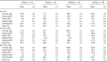
The distribution of density volumes based on the Hounsfield scale (in Hounsfield units (HU)) was obtained from CT images using the VisualPork software package, which was developed for that purpose by the University of Girona and the IRTA (Boada et al., Reference Boada, Spinola, Rodriguez, Martínez and Font i Furnols2009; Bardera et al., Reference Bardera, Martίnez, Boada, Font-i-Furnols and Gispert2012). The cradle was removed from all the images, but the viscera was left. The frequencies of voxels between −1000 and +1400 HU were converted into volumes by means of the DFOV value, the matrix size and the image thickness value, as follows: volume=number of voxels×thickness×(DFOV/512)2. Hounsfield volume distributions were studied further to determine the limits for fat, muscle and bone tissues. From the volume distribution averaged by the target weight in the border region between muscle and bone, the change in slope after the high decrease in the lean area was selected as a cut-off and was set at an HU value of 140 (Supplementary Figure S1). The HU value of 0 was selected as a separation between muscle and fat. Finally, because viscera were included in the images, a cut-off was necessary to separate fat from tissues with less density, such as the lungs or parts of the intestines. In this case, a change in the curve was found at −149 HU because of the inner methodology of the programme for determining the contour of the body, and this value was used as the cut-off. Thus, the partial volumes estimated between −149 and −1, between 0 and 140 and between 141 and 1400 were associated with fat, muscle and bone volumes, respectively, and were used afterwards as independent variables in the regression analysis. Volumes between −1000 and −150 HU, which belong mainly to the less dense parts of the viscera, were considered only in the total volume. The relative carcass lean meat volume (PLean) was calculated as the ratio between the carcass lean meat volume and total carcass volume. Descriptive statistics of the volumes by slaughter weight and genotype are presented in Table 1.
Mean and standard deviation (s.d.) of weights and computed tomography tissue volumesFootnote a obtained in live pigs of three genotypes at different live weight

LD: Landrace; LW: Large White; PI: Pietrain; DU: Duroc.
a VolLean: volume between 0 Hounsfield units (HU) and 140 HU; VolFat: volume between −149 and −1 HU; VolBone: volume between 141 and 1400 HU; TotalVol: volume between −1000 and 1400 HU; PLean: 100×VolLean/TotalVol.
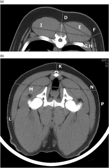
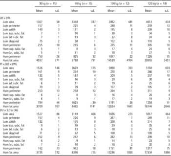
Some physical measurements have been obtained to see whether their inclusion as predictors could reduce prediction error. From an image of the loin between the third and fourth last ribs (Figure 1a – without considering the fals rib), the following six direct physical measurements were obtained: (i) maximum loin width (I); (ii) loin area (G); (iii) loin perimeter (H); (iv) diagonal (maximum length) of the longissimus thoracis muscle (E); (v) lateral subcutaneous fat thickness at the lateral extreme of the longissimus thoracis muscle and perpendicular to the skin (F); and (vi) superior subcutaneous fat thickness at the centre of the dorsal part of the body and perpendicular to the skin (D). From an image of the ham (at the junction of the femur and pubis bones – Figure 1b), the following five direct physical measurements were obtained: (i) width of the ham above the pubis bone (M); (ii) area of the subcutaneous fat of the whole image (L); (iii) lateral subcutaneous fat thickness at the same level as the width measurement (N); (iv) subcutaneous fat thickness at the centre of the dorsal part of the body and perpendicular to the skin (K); and (v) perimeter of the whole image of the ham (P). All lengths and areas were measured in millimetres and square millimetres, respectively. Descriptive statistics of these loin and ham direct physical measurements are presented in Table 2.
Physical direct measurements taken at the loin (a) and ham (b). (D: superior subcutaneous fat thickness; E: diagonal of the longissimus thoracis muscle; F: lateral subcutaneous fat thickness; G: loin area; H: loin perimeter; I: maximum loin width; K: subcutaneous fat thickness at the centre; L: area of the subcutaneous fat; M: width of the ham; N: lateral subcutaneous fat thickness; P: perimeter of the whole ham).

Descriptive statistics (mean and standard deviation (s.d.)) of direct physical measurements (in mm or mm2) taken from whole-animal CT imagesFootnote a

LD=Landrace; LW=Large White; PI=Pietrain; DU=Duroc; sup.=superior; subc.=subcutaneous; lat.=lateral.
a Direct physical measurements used as dependent variables (predictors) in the prediction equations.
Statistical analysis
The relationships between dependent variables (carcass and cuts composition) and independent variables (the CT-measured volume, ratio of volumes or physical measurements) were studied within genotypes, as preliminary analyses showed large differences between the studied genetic lines.
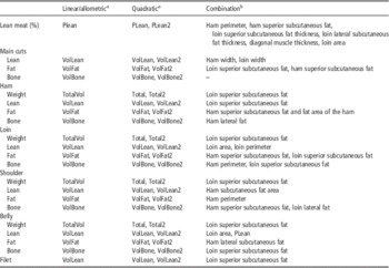
Four different regression approaches, all performed with the REG procedure of the SAS software package (version 9.2; SAS Institute Inc., Cary, NC, USA), were studied. Because of the heteroscedasticity of variances related to the differences in slaughter weight, all the analyses were performed by weighting at each target weight the dependent variables by the inverse of the standard deviation of the residuals (weighted least squares approach). This practice allowed better estimation of the variables of interest within weight groups and adequate distribution of the residuals. The regression approaches studied were the following (see Table 3 for a detailed description of predictors):
-
∙ Linear regressions using CT volumes or CT ratios of volumes as predictors.
-
∙ Quadratic regressions using the previous CT volumes or CT ratios of volumes and their squared value as predictors.
-
∙ Allometric equations (y=ax b linearized as logy=loga+b·logx), in which CT predictors were chosen as for the previous regression models.
-
∙ Linear regression using CT volumes, CT ratios of volumes and direct physical measurements recorded on loin and ham images as predictors. Predictors were selected using the stepwise procedure of SAS (selected criteria: P<0.15) and subjective criteria maximizing the coefficient of determination (R 2) and minimizing root mean square error (RMSE).
Predictors used for each approach

a VolLean: volume between 0 Hounsfield units (HU) and 140 HU; VolFat: volume between −149 and −1 HU; VolBone: volume between 141 and 1400 HU; TotalVol: volume between −1000 and 1400 HU; PLean: 100×VolLean/TotalVol.
b Predictors were the volume or ratio used in the linear approach plus the variables in this column. These variables are not always the same for all the genotypes.
The use of prediction models with only direct physical image measurements was not considered, as previous results showed lower prediction accuracy compared with the use of volumes. Transformation of CT volumes to weight by means of voxel densities was also considered, but preliminary results also showed low prediction accuracy and it was decided to work directly with volumes.
Parameters used to quantify the predictive ability of the equations were the R 2 and the RMSE. Furthermore, the coefficient of variation (CV c ), that is, the percentage of RMSE with respect to the mean, was calculated to make errors comparable.
A cross-validation leave-one-out was used to determine the RMSE of prediction (RMSEPCV) by means of a SAS macro adapted from those presented by Causeur et al. (Reference Causeur, Daumas, Dhorne, Engel, Font i Furnols and Højsgaard2003). The CV p computed as the percentage of RMSEPCV with respect to the mean, was calculated. Equations with the lowest CV p for each trait and genotype were selected.
Results and discussion
The distribution of volumes associated with each HU value by genotype and target live weight is presented in Figure 2. As expected, the volume of live pigs increases as they grow older and heavier. Furthermore, from 70 kg live weight (Figure 2b), a fat peak start appearing (−80 to −120 HU) and grows as pigs gets heavier (Figure2c and d) indicating that fat is deposited at late stages of life. This is corroborated by the fact that some works have shown that the allometric coefficient of fat tissue is higher than one indicating that fat is a late mature tissue (Kouba et al., Reference Kouba, Bonneau and Noblet1999; Landgraf et al., Reference Landgraf, Susenbeth, Knap, Looft, Plastow, Kalm and Roehe2006). It is possible to see differences in the shape of the curve depending on the genotype at each target weight, pointing out that tissue growth patterns differ among genotypes: LD×LW pigs are fatter, PI×(LD×LW) are leaner and DU×(LD×LW) are in between.
Average volumes associated with each Hounsfield value (in Hounsfield units (HU)) in the fat and lean area by genotype at target weights of (a) 30, (b) 70, (c) 100 and (d) 120 kg. Genotypes: LD×LW= Landrace×Large White; PI×(LD×LW)= Pietrain×(Landrace×Large White); DU×(LD×LW)=Duroc×(Landrace×Large White).

Fat and muscle thicknesses, perimeters and areas obtained from CT images taken at specific anatomical positions in live pigs have been proven to be good predictors of carcass traits in young pigs (30 kg live weight; Carabús et al., Reference Carabús, Gispert, Rodriguez, Brun, Francàs, Soler and Font i Furnols2011). Nevertheless, the use of images from the whole animal provides more complete information on its composition and allows more accurate determination of fat, lean and bone volumes for the whole carcass. However, the combination of both types of CT information improve prediction equations of some parameters such as lean meat %, loin weight and loin composition. The relationship between lean, fat and bone of the carcass, obtained by dissection of the four main cuts, and volumes associated with these tissues in CT images of whole live pigs (viscera included) of different genotypes and live weights is very strong (r>0.99 for all the tissues and genotypes, Figure 3). It is strong although: (1) volumes are obtained from live pigs and dissection variables are obtained from cutting and dissection of half carcasses; (2) the live pig images also included white viscera and organs that do not belong in the carcass (some of them are closer to the muscle signal, some others are closer to the fat signal and some others closer to the air signal). The relative weight of white viscera and organs decreases or is kept constant with increasing animal weight, with the exception of flare fat (Font-i-Furnols et al., Reference Font i Furnols, Carabús, Brun, Francàs and Gispert2012). Landgraf et al. (Reference Landgraf, Susenbeth, Knap, Looft, Plastow, Kalm and Roehe2006) also found a constant percentage of heart, spleen and kidney, and a decrease in the percentage of lungs and liver during growth. In the present study, the lungs were almost completely removed from the analysis because of their low density (HU values lower than −140), and in agreement with Landgraf et al. (Reference Landgraf, Susenbeth, Knap, Looft, Plastow, Kalm and Roehe2006) and Font-i-Furnols et al. (Reference Font i Furnols, Carabús, Brun, Francàs and Gispert2012), the proportion of the liver with respect to live body weight was low (2.3% to 2.9% at 30 kg and 1.4% to 1.5% at 120 kg). As explained before, the weights of the lean, fat and bone tissues of the main cuts are strongly related to the corresponding volumes obtained from the CT images of whole live pigs (Figure 3). Further research might be done to determine if scanning of live young piglet could be a good predictor of slaughter performances.
Relationship between the lean (a), fat (b) and bone (c) of the main cuts with the volume of different tissues obtained from the scan of live pigs of different genotypes and weights (r>0.99 for each genotype). Genotypes: black symbols, Landrace×Large White; grey symbols, Pietrain×(Landrace×Large White); white symbols, Duroc×(Landrace×Large White). Target weights: ♦, 30 kg; ▲, 70 kg; ●, 100 kg; ■, 120 kg. HU=Hounsfield units.

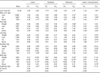
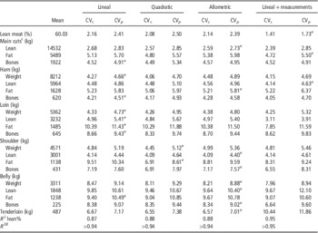
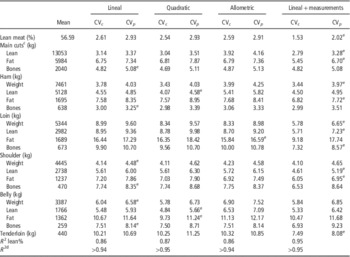
The accuracy of the prediction in terms of relative RMSE (CV c ) and RMSEPCV (CV p ) of carcass composition and cut composition traits for each evaluated model is presented in Table 4 for LD×LW, in Table 5 for PI×(LD×LW) and in Table 6 for DU×(LD×LW). These predictions have been done for each genotype across the different weight categories. The large BW range is responsible for the high R 2 values (0.89<R 2<0.95) observed in all the prediction models. These R 2 values were somewhat lower when estimating lean meat percentage but were always higher than 0.86. In general, differences in CV c between the quadratic and linear models are small, indicating that the inclusion of the quadratic term can seldom improve prediction accuracy. However, when CV p is considered, in general, linear models produced lowest values in comparison with quadratic model, thus, they appear to be more robust. The allometric model yield the lowest CV p values for some of the variables of interest, especially for PI×(LD×LW), although in some cases differences in comparison with the other models do not seem as large. Allometric model is useful for predicting tissue growth with respect to weight (Davies and Pryor, Reference Davies and Pryor1977; Kempster and Evans, Reference Kempster and Evans1979; Kouba and Bonneau, Reference Kouba and Bonneau2009), and also in some traits it can be the best choice for estimating tissue growth from tissue volume obtained by CT. Combining the information provided by tissue volumes and measurements (thicknesses, areas or perimeters) improves the accuracy of some of the predictions, especially for LD×LW and DU×(LD×LW). This effect is very important in the estimation of lean meat percentage of the carcass. This importance makes sense, since in carcass classification, linear measurements of fat and muscle depth is well documented (Font i Furnols and Gispert, Reference Font i Furnols and Gispert2009; Engel et al., Reference Engel, Lambooij, Buist and Vereijken2012). Including physical measurements in the estimation of carcass fat content also reduced the error (CV p between 3.89% and 6.70%). In a recent study, Lambe et al. (Reference Lambe, Wood, McLean, Walling, Whitney, Jagger, Fullarton, Bayntun and Bünger2013) showed correlation coefficients of 0.53, 0.14 and −0.28 between fat thicknesses measured in CT images and, respectively, fat, muscle and bone weights obtained by dissection. Bone weights for the four main cuts have been estimated with similar accuracy in all the studied models.
Coefficients of variation of calibrationFootnote a and validationFootnote b (%) of different prediction models and coefficient of determination (R 2) of overall carcass lean meat and cut weights and tissue weights for Landrace×Large White pigs

RMSE=root mean square error.
a CV c : 100×(RMSE/mean).
b CV p : 100×(RMSE of prediccion by cross-validation−RMSEPCV/mean).
c Ham, loin, shoulder, belly and tenderloin (tenderloin only for lean).
d Rest of the variables.
e Equation with the lowest CV p .
Coefficients of variation of calibrationFootnote a and validationFootnote b (%) of different prediction models and coefficient of determination (R 2) of overall carcass lean meat and cut weights and tissue weights for Pietrain×(Landrace×Large White) pigs

RMSE=root mean square error.
a CV c : 100×(RMSE/mean).
b CV p : 100×(RMSE of prediccion by cross-validation−RMSEPCV/mean).
c Ham, loin, shoulder, belly and tenderloin (tenderloin only for lean).
d Rest of the variables.
e Equation with the lowest CV p .
Coefficients of variation of calibrationFootnote a and validationFootnote b (%) of different prediction models and coefficient of determination (R 2) of overall carcass lean meat and cut weights and tissue weights for Duroc×(Landrace×Large White) pigs

RMSE=root mean square error.
a CV c : 100×(RMSE/mean).
b CV p : 100×(RMSE of prediccion by cross-validation−RMSEPCV/mean).
c Ham, loin, shoulder, belly and tenderloin (tenderloin only for lean).
d Rest of the variables.
e Equation with the lowest CV p .
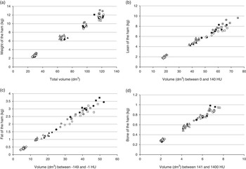
Regarding ham weight, the lowest CV p was obtained with the allometric model for LD×LW genetic line (RMSEP=432 g), with the linear model for the PI×(LD×LW) genetic line (RMSEPCV=382 g) and with the lineal model plus measurements for the DU×(LD×LW) genetic line (RMSEPCV=296 g). Linear, allometric and linear models using physical measurements obtained the lowest CV p for ham lean, fat and bone contents. The CV p of the different ham tissues and ham weight were similar. However, in almost all cases, these errors were slightly higher than those obtained when estimating the tissue composition of the four cuts together. This difference makes sense, because these estimates were obtained from whole-animal images, which are closer to the composition of the four main cuts than to that of only the ham. Nevertheless, different ham tissue weights are highly correlated with the tissue volumes of the whole body of the live pig (r⩾0.99 for the weight and all the tissues for each genotype; Figure 4). However, the errors for loin weight (CV p between 4.73% and 6.65%) were lower than those observed for fat (CP p : 8.44% to 16.59%) and bone (CP p : 8.57% to 9.43%) tissues. In general, CV p was higher for loin than those observed for ham parameters. This difference indicates that whole-body composition presents a higher correlation with ham composition than with loin composition. It also shows that ham composition is a good predictor of whole-body volumes.
Relationship between (a) the weight (kg), (b) the lean (kg), (c) the fat (kg) and (d) the bone (kg) of the ham with the total, lean, fat and bone volume, respectively, obtained from the scan of live pigs of different genotypes and weights (r>0.989 for each genotype). Genotypes: black symbols, Landrace×Large White; grey symbols, Pietrain×(Landrace×Large White); white symbols, Duroc×(Landrace×Large White). Target weights: ♦, 30 kg; ▲, 70 kg; ●, 100 kg; ■, 120 kg. HU=Hounsfield units.

It has been reported that cutting error is greater in the separation of the shoulder from the carcass than in the separation of the ham (Nissen et al., Reference Nissen, Busk, Oksama, Seynaeve, Gispert, Walstra, Hansson and Olsen2006). This can probably explain higher CV p in the shoulder parameters compared with the ham ones. Thus, the obtained CV p values were between 4.48% and 9.48% (RMSE between 184 and 384 g) for shoulder weight, between 4.40% and 8.36% for lean weight, between 6.95% and 9.73% for fat weight and between 5.90% and 8.35% for bone weight.
The belly was the cut for which weight and composition were predicted the worst from whole-pig CT images, although the relative errors were not considerably higher than those for the shoulder. According to Nissen et al. (Reference Nissen, Busk, Oksama, Seynaeve, Gispert, Walstra, Hansson and Olsen2006), the belly produces a high dissection error because of the thin layers of fat and muscle, which are difficult to separate by knife. Additionally, these thin layers may also be the reason for the large number of voxels with partial volume effects, which makes it difficult to assign a given tissue type. There are some differences in the relationship between the lean volume and the weight of the lean of the different cuts. In accordance with the prediction results, this relationship is less precise in the belly than in the other cuts (r>0.98 to 0.99 in the loin and shoulder and r⩾0.97 to 0.99 in the belly, depending on the genotype; Supplementary Figure S2 to S4).
Tenderloin weight error was quite different across the genetic lines. These differences are probably due to the fact that the proportion of fillet in the whole pig body is very small, and consequently, its correlation with whole-body tissue composition is low.
Because of the observed differences in tissue growth patterns, prediction equations were obtained by genotype between 30 and 120 kg BW, and it is worthwhile to see if they fit within weight group. Using the models that yielded the lowest error within genotypes (Tables 4, 5 and 6), prediction equations by weight group was drawn and their respective accuracy was assessed (Table 7 – selected prediction equations are presented in Supplementary Table S2). Lean meat percentage is estimated well for all the slaughter weights, although the accuracy is lower for the lightest carcasses. CT resolution in 30 kg animals probably is better than in heavier pigs, because of lower DFOV applied and lower thickness of the image, thus, this difference in accuracy is probably mainly due to difficulties in applying the European cutting procedures (Walstra and Merkus, Reference Walstra and Merkus1995) and separating the tissues, in particular fat, in 30 kg carcasses. In fact, for the four main cuts, fat tissue shows the highest relative error, with values ranging from 6.42% in the shoulder to 13.97% in the loin. It is also important to note that loin bone and belly bone predictions had lower accuracy in terms of R 2 that was not significant (P>0.05). Loin and belly fat estimates for the 70 kg animals also had a low accuracy, with CV values around 12%. However, in terms of R 2, the lowest accuracy was for loin bone and belly lean weight (R 2<0.16). At the 100-kg target weight, models predicting loin and belly weights did not explain a significant portion of the observed variances. At the 120-kg target slaughter weight, loin weight and bone were predicted much better than at the other target weights, while loin fat was predicted with worst accuracy than at 100 kg. Lambe et al. (Reference Lambe, Wood, McLean, Walling, Whitney, Jagger, Fullarton, Bayntun and Bünger2013) also found higher R 2 values between dissected and CT-predicted fat, muscle and bone of the carcass side with increasing live weight (60, 85 and 115 kg). Moreover, all the belly parameters estimated in the present study also had higher or similar accuracy at the 120 kg target weight than at the others. This can be explained with the fact that heavier carcasses are easier to cut and dissect, although that does not seem to be the case with the shoulder. In fact, only the models predicting shoulder weights at the 120-kg target slaughter weight did not explain a significant portion of the observed variation, probably because, as reported by Nissen et al. (Reference Nissen, Busk, Oksama, Seynaeve, Gispert, Walstra, Hansson and Olsen2006), cutting error is the highest for this cut.
Coefficient of variation (CV)Footnote a and coefficient of determination (R 2)Footnote b calculated within weight groups using prediction equations yielding the lower prediction error within genotypes and across weight groups

a 100×root mean square error/mean.
b R 2-values in italics are not significant (P>0.05).
c Ham, loin, shoulder, belly and tenderloin (tenderloin only lean).
Conclusions
There is a very good relationship between cross-sectional CT images obtained in live growing female pigs of different genotypes (including viscera) and carcass and main cuts composition. For this reason, measurements taken on CT images of whole-animal in vivo allow accurate estimation of carcass lean meat percentage as well as the weight and tissue composition of cuts in pigs from 30 to 120 kg BW, using empirical regression equations. The prediction accuracy varied across genotypes, variables of interest and BW. Linear models using CT tissue volumes as predictors, allometric models or linear models using CT tissue volumes and physical measurements at specific anatomical positions of the animal body, were in general more robust than quadratic models. However, further work is needed to allow the accurate prediction of pig cut weights and composition using reconstructed 3D pig CT images from which the whole animal body is virtually cut and dissected, thus mimicking dissection by the butcher, in an attempt to render prediction accuracy independent of pig genetic traits and BW. Also more work is needed to build growth models that would allow relate live young piglet CT images with carcass composition at slaughter.
Acknowledgements
The present study was supported by the Instituto Nacional de Investigaciones Agrarias –INIA (Evaluación in vivo del crecimiento alométrico de los tejidos muscular y adiposo de los cerdos según la genética y el sexo mediante tomografía computerizada. RTA2010-00014-00-00). INIA is also thanked for the scholarship to Anna Carabús. The authors wish to thank Albert Brun, Carles Francàs, Albert Rossell, Agustí Quintana, Albert Fontquerna, Carlos Millán y Alfons Varas for their invaluable technical assistance.
Supplementary material
To view supplementary material for this article, please visit http://dx.doi.org/10.1017/S1751731114002237