


1 Introduction
Methodologists urge researchers to test observable implications of assumptions that aid causal inference. In natural experiments and related designs, researchers often report covariate balance tests. The logic appears straightforward: if a coin flip had determined treatment assignment, pre-treatment covariates or “placebo outcomes” would have the same distribution, in expectation, in treatment and control groups (Caughey, Dafoe, and Seawright Reference Caughey, Dafoe and Seawright2017; Eggers, Tuñón, and Dafoe Reference Eggers, Tuñón and Dafoe2023). A statistically insignificant association between treatment and covariates is consistent with random assignment—an important advantage, if true, for making inferences about causation—while a significant association may suggest a flaw in the design.
Unfortunately, these widely used tests may shed no light on key identification conditions. Researchers testing the validity of an alleged natural experiment would like to know whether a treatment is assigned independently of potential outcomes—a condition sometimes called “as-if” random.Footnote 1 In many studies, however, none of the measured covariates used in the balance tests are prognostic, that is, associated with potential outcomes. In others, some covariates are prognostic but others are not. As we show in this article, balance tests based on irrelevant covariates unrelated to potential outcomes cannot tell us whether as-if random is plausibly met. A similar point applies to regression-discontinuity (RD) designs, in which analysts often seek to test the continuity of potential outcomes at a threshold determining treatment assignment, rather than as-if random. The continuity of non-prognostic covariates is uninformative about the continuity of potential outcomes themselves.
Using a sample of experiments, natural experiments and RD designs published in top political science journals, we demonstrate three features—and, we argue, problems—of existing balance tests: (1) covariate prognosis is rarely or never measured; (2) the overall prognosis of the covariates used in balance tests varies across studies—and is often very weak; and (3) within studies, the prognosis of individual covariates also varies and is also often weak.
These problems undermine the ability of standard balance tests to assess identification conditions. In typical practice, researchers report lengthy covariate balance tables without considering which variables are actually predictive of outcomes. However, sometimes imbalances occur on irrelevant covariates unrelated to potential outcomes. Other times, it is the prognostic covariates that are imbalanced. Because prognosis is not measured or incorporated formally into tests, the varied informativeness of different covariates is not considered, and it is difficult to assess how meaningful are rejections for any individual covariate. Moreover, because researchers often present tests for different covariates separately, standard procedures also lead to multiple testing problems as well as indeterminacy: there is no clear rule for rejecting an overall null hypothesis like as-if random. Finally, because researchers do not report the joint prognosis of covariates, readers and reviewers cannot readily assess the overall power of the tests to falsify identification conditions.
We make several contributions in this article to addressing these common problems. First, we show why covariate prognosis is important for balance tests. We demonstrate that tests using irrelevant, non-prognostic covariates can lead researchers falsely to reject as-if random when it is true or to fail to reject when it is false.
Second, we show that researchers can increase the power and specificity of their tests by measuring the most jointly prognostic covariates possible—and then prioritizing the most informative covariates, among those they measure. Here, we build on and extend research in statistics and epidemiology on “prognostic scores,” which have been little used in the social sciences (see especially Hansen Reference Hansen2008 and Stuart, Lee, and Leacy Reference Stuart, Lee and Leacy2013).Footnote 2 Thus, we offer the following concrete advice for how researchers using balance tests can address problems (1)–(3) highlighted above:
-
(1) Measure and report prognosis in balance tests: We propose measures of covariate prognosis that help researchers and readers assess the informativeness of balance tests. Although potential outcomes are partially unobservable (Holland Reference Holland1986), it is possible to assess, for instance, how well covariates predict potential outcomes under control using data from a control group sample. Such diagnostic measures are essential because prognosis is an empirical question. For example, while the pre-treatment values of outcome variables tend to be related to potential outcomes under control (Imbens and Rubin Reference Imbens and Rubin2015, 483–484), such lagged outcomes may or may not be available to researchers; and, as we show, in some applications they are not in fact prognostic.
-
(2) Maximize overall covariate informativeness: Our results show that as the set of covariates used in balance tests become more prognostic, the tests become more powerful and specific. Thus, researchers should endeavor to collect data on the most jointly prognostic covariates possible. Theoretical and substantive knowledge can guide the identification of covariates that are likely associated with potential outcomes in a given context. Where feasible, researchers should include the lagged dependent variable as a covariate. Formalizing the reporting of measures of prognosis as part of the publication process, per (1), can aid assessment of informativeness and heighten researchers’ incentives to gather data on the most predictive covariates possible.
-
(3) Prioritize prognostic variables in the tests: Finally, we construct balance tests that give greater weight—among a set of measured covariates—to the individual variables most associated with potential outcomes. By combining information on prognosis across covariates into a single test statistic, these prognosis-weighted tests confront problems of indeterminacy and multiple testing in covariate-by-covariate tests and can increase the power and specificity of tests.
For (3), the key test statistic is the difference in the average fitted, covariate-adjusted potential outcomes under control across treatment and control groups. As in Hansen (Reference Hansen2008) and Stuart et al. (Reference Stuart, Lee and Leacy2013), the researcher thus uses a technique to learn predicted potential outcomes in the control group, obtain predictions for potential outcomes for units in the treatment group, and compare averages of the two fitted values. In our baseline test of as-if random, the statistic is equivalent to a weighted difference of covariate means across treatment and control groups; the weights are coefficients from a standardized linear regression of control group outcomes on covariates and measure prognosis. The test thus combines the inputs of standard balance tables—differences of means of individual covariates—into a prognosis-weighted statistic with a single associated p-value. This omnibus approach addresses indeterminacy and multiple testing problems, while upweighting informative covariates and downweighting irrelevant covariates unrelated to the outcome.
We also extend prognosis weighting in several ways. First, we adapt the technique for RD designs. To test the continuity of average potential outcomes at the threshold determining treatment assignment, researchers may compare differences of prognosis-weighted intercepts from regressions above and below the threshold. This approach similarly prioritizes the most informative covariates and bases assessment on a single prognosis-weighted statistic.
Second, we expand the fitted value approach to flexible regressions and nonlinear machine learning methods, which to our knowledge existing work on prognostic scores has not done. We use simulations to assess how prognosis weighting can improve power and specificity, relative to standard unweighted tests, and to compare the different fitting procedures.
Third, for hypothesis testing, we provide a bootstrap that accounts for the statistical dependence of covariate control group means and the estimated prognosis weights. We also discuss how to leverage equivalence testing with prognosis weighting. We implement all statistical routines in our forthcoming R package pwtest.Footnote 3
Our results show that prognosis-weighted tests can achieve substantial gains in power as well as specificity, relative to standard unweighted tests. The key advantage is that downweighting irrelevant noise variables unrelated to potential outcomes can limit both false positives and false negatives—because conclusions are then based on the most informative covariates. Linear prognosis-weighted tests with expanded polynomial bases or covariate interactions tend to perform best in our simulations, in terms of simultaneously achieving the greatest power and specificity.
Finally, we discuss many empirical examples of problems (1)–(3) in applied research. Both the extent of imbalance and, especially, the degree of covariate prognosis vary across the studies in our sample. We report p-values for prognosis-weighted tests of as-if random and continuity and show graphically how our prognosis-weighted tests project out irrelevant covariates. This helps demonstrate how prognosis weighting can address the problems we highlight. The techniques extend naturally beyond natural experiments and discontinuities to randomized experiments with attrition, imperfect implementation or other issues that may be detectable with tests based on covariate imbalance, once analysts have outcome data available.
Our survey of applications demonstrates that by properly prioritizing informative covariates, prognostic-weighted tests base conclusions on the variables most predictive of outcomes. In one set of studies, the relatively predictive individual covariates are imbalanced (e.g., Samii Reference Samii2013, Blattman Reference Blattman2009, or Thomas Reference Thomas2018); here, prognosis weighting can lead to rejections of as-if random, whereas unweighted tests do not. In a second set (e.g., Boas and Hidalgo Reference Boas and Hidalgo2011; Kim Reference Kim2019; Novaes Reference Novaes2018), there is imbalance only on irrelevant noise covariates, so adjusting for prognosis may increase our confidence in the validity of the natural experiment. In a final set of studies (e.g., Fouirnaies and Hall Reference Fouirnaies and Hall2014), there is a mix of observed balances and imbalances on prognostic and non-prognostic variables, and prognosis weighting helps sort out the relative importance of the different covariates.
We also show the importance of covariate prognosis for testing the randomness of close elections, a topic of important debate (Caughey and Sekhon Reference Caughey and Sekhon2011; De la Cuesta and Imai Reference De la Cuesta and Imai2016; Eggers et al. Reference Eggers, Fowler, Hainmueller, Hall, James and Snyder2015; Hartman Reference Hartman2021). Existing tests exhibit the general problems (1)–(3) we identify. Using data from the U.S. House, we demonstrate how prognosis-weighted tests synthesize and extend contrasting previous results. Most importantly, we show that covariate prognosis in cross-national tests of the randomness of close elections is very weak: for example, lagged party incumbency has on average no predictive value for incumbency outcomes in cross-national data. Balance tests using this single covariate, as in Eggers et al. (Reference Eggers, Fowler, Hainmueller, Hall, James and Snyder2015), therefore have little power to falsify as-if random or continuity. In particular, they are prone to false negatives. This case study therefore not only suggests that the methodological debate on the randomness of close elections in general is not settled but also highlights the importance of empirically measuring prognosis—rather than assuming it—and accounting for it analytically in identification tests.
Methodologically, by incorporating prognosis-weighting into omnibus tests of identification conditions, we contribute to previous research on covariate balance testing. Imai, King, and Stuart (Reference Imai, King and Stuart2008) emphasize the problem that failing to reject a null hypothesis is not the same as accepting it: researchers may fail to reject simply because their study is small and underpowered. Our work adds a further dimension to this “balance test fallacy,” because we show that even a large, apparently well-powered test will not validly test key identification conditions if covariates are not prognostic. By basing tests on a single summary test statistic, we also provide a new way to address multiple testing concerns (De la Cuesta and Imai Reference De la Cuesta and Imai2016) and complement valuable articles on omnibus covariate balance tests (Caughey et al. Reference Caughey, Dafoe and Seawright2017; Gagnon-Bartsch and Shem-Tov Reference Gagnon-Bartsch and Shem-Tov2019; Hansen and Bowers Reference Hansen and Bowers2008), which do not however consider covariate prognosis.Footnote 4
Our most important contribution, however, is practical. Social science researchers deploying balance tests in natural experiments and related designs do not currently measure or account for the informativeness of covariates. We show how (1) measuring and (2) maximizing joint prognosis, then (3) prioritizing informative covariates that are predictive of outcomes while de-prioritizing irrelevant ones, can improve the usefulness of covariate balance tests. Prognosis-weighted tests offer an improvement on current practice in applied research—which ignores the issue of prognosis entirely—and can lead to more credible conclusions about whether identifying conditions are met.
In the next section, we use our sample of papers from top political science journals to illustrate the three key problems we highlight. We then discuss in Section 3 why prognosis matters for testing identification conditions. In Section 4, we describe bootstrap prognosis-weighted tests of as-if random and adapt the approach to test continuity of potential outcomes in RD designs. We also discuss simulation evidence on the tests’ power and specificity. In Section 5, we turn to practical issues, discussing many examples that show the gains from prognosis weighting and developing the case study of close elections. Our conclusions in Section 6 expand on our recommendations for practice. Technical details and formal arguments are in the Supplementary Material.
2 The problem of weak covariate prognosis: A survey of reported balance tests
To motivate our focus, we study a random sample of 150 articles that use randomized experiments, natural experiments and RD designs and that were published in three top political science journals (the APSR, the AJPS and the JOP), stratifying by journal, over the time period 2000–2019.Footnote 5 Overall, 52% percent of articles present balance tests.
The survey suggests three features—and, we will argue, problems—of standard balance tests.
2.1 Prognosis is rarely measured
Covariate prognosis is rarely considered systematically. In fact, we found no examples of efforts to measure the prognosis of the covariates used in balance tests.
This is a critical omission because different covariates vary in their ability to predict potential outcomes. As we discuss next, (a) the set of covariates used in a given study may or may not be jointly prognostic and (b) within a given study, different individual covariates may have different degrees of association with the outcome variable.
Moreover, it is not obvious a priori whether a given set of covariates is prognostic. For example, methodologists sometimes recommend using the pre-treatment value of the dependent variable as a covariate (Imbens and Rubin Reference Imbens and Rubin2015, 483–484; Caughey et al. Reference Caughey, Dafoe and Seawright2017; Eggers et al. Reference Eggers, Tuñón and Dafoe2023). This may be because it can be highly prognostic of potential outcomes under control. Yet this also might not hold, for example, due to heterogenous temporal trends or other factors. In our case study of close-election designs later, we show that lagged party incumbency has almost no predictive value for incumbency outcomes in a cross-national data set. Prognosis is thus an empirical question, and it requires formal diagnosis.
Reporting measures of the association between covariates and outcomes can give readers an indicator of the informativeness of balance tests. As we will show, prognosis powerfully affects the ability to use covariate balance to test key identification conditions meaningfully (Sections 3 and 4). However, such measures are essentially never reported in applied work.
2.2 Joint covariate prognosis varies across studies—and is often weak
The joint prognosis of covariates used in balance tests in fact varies substantially across different studies—and is often quite low.
The horizontal axis of Figure 1 plots the
$R^2$
 from the multiple regression of control group outcomes on all available covariates, for a sub-sample of the studies (“Prognosis
$R^2$
 ”).Footnote
6
As we discuss later, such goodness-of-fit measures provide one helpful tool for assessing prognosis. The vertical axis plots the multiple
$R^2$
 from the regression of a treatment assignment indicator on all available covariates (“Imbalance
$R^2$
 ”).
Imbalance versus prognosis in balance testing (sample of natural experiments and RD designs).
Note: The figure plots a sample of natural experiments and regression-discontinuity (RD) designs drawn from all those published in the American Political Science Review, American Journal of Political Science and Journal of Politics, 2000–2019; Caughey and Sekhon (Reference Caughey and Sekhon2011) is added. Prognosis
$R^2$
 comes from a regression of potential outcomes under control on all available covariates (control group only). Imbalance
$R^2$
 comes from a regression of treatment assignment on all available covariates. Two studies we discuss in detail in Section 5 are bolded. See Section 1 of the Supplementary Material for further information.

Figure 1 Long description
A scatter plot with the horizontal x-axis labeled Prognosis R-squared ranging from 0.0 to 0.6 and the vertical y-axis labeled Imbalance R-squared ranging from 0.0 to 0.4.
Data points are distributed as follows:
* At the origin (0,0) is a bolded black dot labeled Eggers et al. (2015).
* Clustered near the bottom-left (low prognosis and low imbalance) are several light gray dots including Holbein and Hillygus (2016), Klasnja (2015), Healy and Malhotra (2013), Blattman (2019), and Fourniaies and Hall (2014).
* Moving toward the center are Samii (2013) and Hidalgo and Nichter (2016).
* In the upper-left quadrant, Thomas (2018) shows high imbalance (above 0.4) with low prognosis (around 0.15).
* In the center-left, Boas and Hidalgo (2011) sits at approximately 0.15 prognosis and 0.2 imbalance.
* In the upper-right quadrant, Caughey and Sekhon (2011) is marked with a bolded black dot at approximately 0.5 prognosis and 0.3 imbalance.
* Further right are Novaes (2018), Kim (2019), and Hall (2015), the latter having the highest prognosis value at over 0.6.
Figure 1 suggests several insights. First, we find relatively little covariate imbalance in these studies overall. Most cluster along the bottom portion of the plot, with a low Imbalance
$R^2$
 (less than 0.1). This likely reflects our sampling strategy: studies with substantial covariate imbalance are unlikely to be published as natural experiments or discontinuity designs. Sampling a fuller range of observational studies would presumably populate the top part of the figure.
Second and more concerningly, however, covariates are not predictive of potential outcomes in many studies. Some studies located toward the right of the horizontal axis use covariates associated with potential outcomes. Yet, many studies cluster close to the vertical axis—where the prognosis
$R^2$
 is zero. We note that in the full sample of 150 studies, only 18% of balance tests used the pre-treatment value of the dependent variable as a covariate.
Thus, many balance tests use noise covariates that are only weakly related to potential outcomes. This includes several studies with good observed balance. Arguments we will develop in Sections 3 and 4 suggest that heuristically, there are four kinds of cases in Figure 1:
-
1. In the lower-left quadrant, we risk a form of Type I error: we may fail to reject as-if random due to the observed balance of noise covariates unrelated to outcomes. Yet potential outcomes are themselves related to treatment assignment.
-
2. In the upper-left quadrant, we may instead be prone to spurious rejection of as-if random—because there is imbalance on covariates unrelated to potential outcomes.
-
3. In the lower-right quadrant, we find cases with high prognosis but low imbalance: here, the claim of as-if random may be most persuasive.
-
4. Finally, in the upper-right quadrant, rejection may be most persuasive of a failure of as-if random—because imbalanced covariates are as a whole prognostic of potential outcomes.
For 3 and 4, however, we note that covariates may be associated with potential outcomes as a whole, leading to a high prognosis
$R^2$
 ; yet balance or imbalance could occur on a non-prognostic subset of covariates.
This implies that tests should be based on the most individually prognostic covariates in the set, as in the prognosis-weighted procedures we present in Section 4.
2.3 Individual covariate prognosis varies within studies—and is also often weak
Finally, within studies, different covariates also vary in their informativeness about outcomes.
In Figure 2, we plot (a) the standardized difference of means across treatment and control groups for each covariate in each study in Figure 1 (vertical axis) against (b) that covariate’s individual prognosis, that is, the standardized regression coefficient from the prognosis regression (horizontal axis). The black dots indicate differences of means that are statistically significant in a t-test, while gray dots indicate insignificant differences.Footnote 7
The prognosis and imbalance of individual covariates varies.
Note: For each of our sampled studies in Figure 1, we plot for each covariate the standardized difference of means across treatment and control (vertical axis) against the covariate’s standardized multiple regression coefficient from the prognosis regression (horizontal axis). The triangle indicate the overall prognosis and imbalance
$R^2$
 s. We indicate in black the covariates where the p-value
$\leq 0.05$
 from a two-tailed t-test of covariate values across treatment and control, suggesting covariate imbalance. In discontinuity designs, we use the authors’ chosen bandwidths to define the study group for the tests (see Section 1.1.1 of the Supplementary Material for details).

Figure 2 Long description
A grid of 14 scatter plots arranged in two columns and seven rows. Each plot shares a common Y axis labeled Covariate difference in means (standardized) and a common X axis labeled Covariate prognosis. Dashed lines intersect at the origin (0,0) in each plot. Data points are represented by light gray circles, black circles (indicating p-value less than or equal to 0.05), and a single red triangle representing the overall prognosis and imbalance.
* Caughey and Sekhon (2011): Points clustered near the Y axis. Red triangle at approximately (0.5, 0.3).
* Eggers et al. (2015): Points concentrated at the origin. Red triangle at (0, 0).
* Blattman (2019): Points spread horizontally. Red triangle at (0.2, 0.05).
* Boas and Hidalgo (2011): Points scattered around the origin. Red triangle at (0.15, 0.2).
* Thomas (2018): Points clustered near the Y axis with one outlier at (0, 4). Red triangle at (0.18, 0.6).
* Fourniaies and Hall (2014): Dense cluster around the origin. Red triangle at (0.15, 0.05).
* Hall (2015): Points spread from -1.0 to 1.0 on the X axis. Red triangle at (0.6, 0.4).
* Healy and Malhotra (2013): Points scattered in all quadrants. Red triangle at (0.15, 0.05).
* Hidalgo and Nichter (2016): Vertical cluster along the Y axis. Red triangle at (0.4, 0.08).
* Holbein and Hillygus (2016): Points tightly clustered at the origin. Red triangle at (0.02, 0.01).
* Kim (2019): Points spread from -0.2 to 0.6 on the X axis. Red triangle at (0.55, 0.1).
* Klasnja (2015): Points concentrated on the Y axis with outliers at -2.5 and 2.5. Red triangle at (0.1, 0.08).
* Novaes (2018): Points spread horizontally. Red triangle at (0.45, 0.18).
* Samii (2013): Points spread from -0.5 to 0.3 on the X axis. Red triangle at (0.25, 0.08).
As Figure 2 shows, some individual covariates are strongly predictive of potential outcomes—while for many others, the prognosis coefficient is near zero. Furthermore, as with joint prognosis (Figure 1), the relationship between individual prognosis and the treatment-control imbalances varies. In some studies, irrelevant covariates unrelated to potential outcomes are imbalanced; other times, it is the prognostic covariates that are significantly imbalanced.
Unfortunately, as with joint prognosis, we find no formal measurement in these studies of which particular covariates are actually predictive of outcomes. Absent a plot like Figure 2 or other measures of the prognosis of individual covariates, it is difficult to know which ones are informative.
This situation appears typical in the literature. Researchers often present tests for numerous individual covariates: the majority of the studies in our sample that present balance tests (56%) report only covariate-by-covariate tests. Such tests can result, however, in indeterminacy (Kost and McDermott Reference Kost and McDermott2002) as well as problems of multiple statistical comparisons (Benjamini and Hochberg Reference Benjamini and Hochberg1995; De la Cuesta and Imai Reference De la Cuesta and Imai2016). Rules of thumb—such as that only 1 out of 20 differences should be significant at the 0.05 level when treatment is randomized—do not apply when covariates are correlated and thus tests are dependent, as they almost always are in practice (Caughey et al. Reference Caughey, Dafoe and Seawright2017). Results of disparate covariate-by-covariate tests fail to lead to a clear decision rule for rejecting an overall null hypothesis like as-if random.
Most worrisome, different covariates differ in their informativeness about potential outcomes—yet because prognosis is undiagnosed, it is difficult to know which of the separate covariate-by-covariate tests should be treated as most dispositive. This variation in individual informativeness affects interpretation of test results, as we will show. Even studies that assess the joint imbalance of all covariates using omnibus or global test statistics—for example, by reporting the p-value of the F-statistic from the (unweighted) regression of a treatment indicator on all covariates—do not account for the varied informativeness of individual covariates.Footnote 8 All covariates are thus treated equally in balance tests—but in truth, some are more informative than others.
2.4 Summary of survey: Limitations of standard balance tests
Our survey shows that covariate prognosis varies both within and across published balance tests. Yet, in none of the studies we examined is prognosis measured. Nor is it incorporated formally into tests.
What are the implications for our conclusions about identification conditions? How should we think about tests with low imbalance but also low prognosis, as in the bottom-left quadrant of Figure 1? What inferences can we draw from those located in the figure’s other quadrants? And how should we adapt covariate balance tests to account for the unequal informativeness of different covariates?
We develop theory and simulations to address these questions in Sections 3 and 4, then we return to further discussion of empirical examples in Section 5.
3 Are potential outcomes balanced? Why prognosis matters
Researchers using experiments, natural experiments and discontinuity designs often wish to test key identification conditions.
In valid natural experiments, the following condition must hold.
Assumption 1 As-if Random Assignment
Treatment is assigned independently of potential outcomes.
As-if random ensures, for example, that sicker patients do not go systematically to the treatment group in a drug trial studying health outcomes, or that those more prone to vote do not disproportionately receive a vote-mobilizing intervention.Footnote 9 If as-if random holds, the true ATE is estimable using simple, transparent methods (Freedman Reference Freedman1999).
This assumption can be the “Achilles Heel” of natural experiments, however (Dunning Reference Dunning2008). In a true randomized experiment, a chance protocol under the control of a researcher (Fisher Reference Fisher1935) ensures that treatment is independent of potential outcomes, as well as any fixed covariates—though even in experiments, issues like attrition or failed implementation can compromise as-if random. In natural experiments, by contrast, as-if random is held to be an implication of a process, not under the control of the researcher, that is alleged to produce a haphazard allocation that does not depend on potential outcomes.
Unfortunately, Assumption 1 cannot be directly verified due to the “fundamental problem of causal inference” (Holland Reference Holland1986): we do observe treatment potential outcomes for those assigned to the control group, and vice versa. We thus cannot use the realized distribution of potential outcomes to test as-if random.
3.1 What standard balance tests do
Researchers therefore seek to test Assumption 1 using information about the realized distribution of observed covariates across treatment and control groups. The difficulty is that these covariates may or may not be related to potential outcomes—and thus standard balance tests may or may not effectively test as-if random.
Suppose that the space of possible covariates contains “signal” covariates, which contain all information about potential outcomes, and “noise” covariates, which contain none (compare Liu and Ruan Reference Liu and Ruan2020). Signal covariates and potential outcomes are dependent, while noise covariates are independent of potential outcomes.Footnote 10
The logic of standard balance tests appears to rest on the following claim.
Claim 1. Treatment assignment is independent of covariates if and only if treatment assignment is independent of potential outcomes.
Thus, a failed balance test suggests a failure of as-if random, and vice versa.
The claim is false, however. As we show formally in Section 2 of the Supplementary Material, two kinds of counterexamples are relevant.
Counterexample to Claim 1: False positives. Suppose treatment is assigned independently of potential outcomes, so as-if random holds. However, observed covariates are merely noise, and Nature has adversarially chosen to assign treatment so that it depends on the noise covariates. Then treatment assignment depends on covariates—even though treatment is assigned independently of potential outcomes. The “if” direction of the claim thus does not follow.
For example, in an observational study of the efficacy of a new drug, men might tend to select into the treatment group. Yet gender may be unrelated to health status or responsiveness to the treatment. If we have only data on gender, we may wrongly reject as-if random based on the covariate imbalance, even though potential outcomes themselves may be independent of treatment.
A researcher who believed Claim 1 might thus perform a balance test, observe imbalance between treatment and control groups on some subset of covariates, and conclude that treatment was not randomly assigned. However, this is a false positive if the imbalanced covariates are unrelated to potential outcomes: their imbalance does not constitute evidence that as-if random fails.
Conversely—and perhaps most importantly, as we might worry most about false claims to a natural experiment—balance on a spurious covariate does not imply that treatment is assigned independently of potential outcomes, as the next counterexample shows.
Counterexample to Claim 1: False negatives. Assume now that as-if random fails but treatment is assigned independently of the noise covariates. Independence of observed noise covariates and treatment does not therefore imply that treatment is assigned independently of potential outcomes. The “only if” direction of Claim 1 does not follow.
For instance, sicker patients might select into the treatment group. As-if random may thus fail. Health after an intervention may be closely related to prior health—yet we may fail to measure this signal covariate. In contrast, men may be as likely to select into treatment as women, leading to expected balance on gender. Yet, if gender is not related to potential outcomes or responsiveness to treatment, its observed balance cannot readily validate as-if random. If we base a balance test on gender, we may thus falsely fail to reject as-if random.
In sum, covariates differ in their informativeness about potential outcomes. If we only measure noise covariates—those unrelated to potential outcomes—then finding balance or imbalance on those covariates does not allow us to test as-if random assignment.
3.2 The power of prognosis
The discussion thus far suggests we should consider the informativeness of covariates when constructing balance tests.
There are at least two reasons that prognosis of covariates matters for testing—and also thus why covariates with differing degrees of prognosis should not be “treated equal.”
First, as mentioned, the most direct test of as-if random would assess balance of potential outcomes across the treatment and control groups (Imbens and Rubin Reference Imbens and Rubin2015, Chapter 21). This test is impossible: once treatment has occurred, we do not observe potential outcomes under control in a treatment group or potential outcomes under treatment in a control group (Holland Reference Holland1986).
Yet, a covariate strongly associated with potential outcomes may give us substantial information about this realized balance. Indeed, as we discuss next, if the covariates at our disposal happened to contain all information about subjects’ potential outcomes, then we could use the observed balance of covariates to validly test the independence of treatment assignment and potential outcomes.
Second and relatedly, if subjects self-select into treatment groups, as in many observational studies, then (contra as-if random) the intervention they receive may depend on the outcomes they would experience in each group (Angrist and Pischke Reference Angrist and Pischke2009; Heckman Reference Heckman1979). Agents may have unobserved prognostic information that researchers lack, for example, about their expected gains from treatment that may lead them select into treatment. The informativeness of balance tests can therefore be especially limited if covariates are not predictive of potential outcomes.
In contrast, as we argue next, measuring and prioritizing prognostic covariates in tests is most likely to detect such selection into treatment on the basis of potential outcomes.
3.2.1 A conceptual motivation: Minimally sufficient covariates
As a conceptual motivation for this argument, suppose first that observed covariates that are “minimally sufficient”—essentially, they contain all and only the possibly observable information about potential outcomes (Dawid Reference Dawid1979). In this case, as we show in the Supplementary Material, treatment assignment depends on the covariates if and only if they depend on potential outcomes (Section 3.1 of the Supplementary Material and Theorem A.1 in the Supplementary Material). Then, we may validly reject as-if random based on the non-independence of treatment assignment and covariates—as in standard balance tests.
This idea is useful because it underscores the importance of choosing jointly informative covariates—and then prioritizing the most informative subset for tests. Sufficiency only guarantees the “if” direction of Theorem A.1 in the Supplementary Material. Thus, it controls false negatives: if covariates are sufficient, then when treatment is not assigned independently of potential outcomes, we should expect a well-powered balance test to fail. For the “only if” direction, we need minimum sufficiency—that is, the and only part of its definition. This controls false positives: if covariates are minimally sufficient, a failed balance test implies a failure of as-if random. This is a key motivation for the prognosis-weighted tests we discuss in Section 4. By projecting potential outcomes onto covariates before running tests, we effectively discard uninformative covariates—as in the creation of a minimally sufficient from a merely sufficient covariate set.
In applications, unfortunately, covariates usually cannot be expected to contain such complete information about the values of potential outcomes. Moreover, sufficiency is difficult or impossible to validate. To be sure, a version of this condition could occur in some settings. For example, the pre-treatment value of the response variable may sometimes equal the post-treatment value in the absence of an intervention. Then this covariate’s correlation with potential outcomes under control is 1, which also implies sufficiency. Yet, even with a lagged dependent variable, temporal trends could imply differences in values of the outcome variable in the pre- and post-treatment periods, absent an intervention. These trends could be heterogeneous for different units, which implies a correlation less than 1. The direct practical implications of the minimal sufficiency theorem are thus limited.
3.2.2 The importance of prognosis
The more prognostic covariates are, however, the closer they may get to approximating the ideal situation of complete informativeness, that is, sufficiency. The logic suggests that the power and specificity of tests will improve as covariates become more predictive of potential outcomes.
Moreover, even when a set of measured covariates is not sufficient, we may be able to improve the performance of tests by prioritizing the individual covariates that are most closely associated with potential outcomes. We discuss simulation evidence that supports this claim in Section 4.2.
This argument parallels in some ways standard arguments about the role of prognosis in achieving control over confounding variables in observational studies (VanderWeele and Shpitser Reference VanderWeele and Shpitser2011, Reference VanderWeele and Shpitser2013): the more predictive of outcomes the measured covariates are, the less likely it is that unobserved factors produce violations of as-if random. The difference is that here we are focusing on covariate characteristics that allow us effectively to test as-if random, rather than control for violations of it. Testing and estimation can be complementary tasks. However, as we suggested in Section 3.1, with balance testing we should be attentive to both false negatives and false positives: we may fail to reject as-if random because spurious covariates are balanced, but we may also falsely reject it because irrelevant covariates are imbalanced.
The challenge is therefore to collect covariate data that allow us to test identification conditions convincingly. Unfortunately, the predictiveness of covariates for outcomes has been ignored in applications of balance testing in experiments, natural experiments and discontinuity designs. As we emphasized in Section 2, researchers do not typically report measures of covariate prognosis, nor do they discuss efforts to maximize the informativeness of covariates used in balance tests. Thus, it is usually difficult to assess the extent to which these pathologies of standard balance tests apply.
In sum, we argue that researchers should attempt to gather the most informative set of covariates possible, and then prioritize the most prognostic ones in their tests. The more prognostic are covariates, the more information they give us about the likely balance of potential outcomes, and the more useful are covariate balance tests. Measures such as the prognosis
$R^2$
 (Figures 1 and 2) can be viewed as a continuous operationalization of informativeness. Such measures can help researchers assess the adequacy of information about potential outcomes contained in a set of measured covariates. We return to this point in connection with our simulations (Section 4.2), where we assess how error rates in tests vary as a function of levels of prognosis observed in the empirical studies in Figures 1 and 2.
4 Prognosis-weighted covariate balance tests
Suppose researchers successfully gather data on jointly prognostic covariates, as recommended in the previous section. How should they combine the information from different covariates to test key identification conditions?
Prognosis-weighted tests provide a useful approach that prioritizes the covariates that are most informative about potential outcomes. Hansen (Reference Hansen2008) proposed balancing on “prognostic scores” in observational studies, and some subsequent literature has explored the performance of prognostic-score balancing using simulations (see especially Stuart et al. Reference Stuart, Lee and Leacy2013).
We extend these methods to develop covariate balance tests appropriate for assessing as-if random (Assumption 1) as well as continuity of potential outcomes in RD designs (see Section 4.1.1). The key test statistic in all tests is a difference in the average covariate-adjusted potential outcome under control—that is, a difference of fitted values—across treatment and control groups. We define this statistic formally in Section 4.1 of the Supplementary Material.
In a baseline test of as-if random based on linear regression, this statistic is equivalent to a weighted combination of differences of covariate means, where the weights are coefficients from the prognosis regression—that is, the standardized multivariate regression of outcomes on covariates in the control group. Thus, the test takes the usual inputs of covariate balance tests—covariate differences of means across treatment and control—and combines them into a single test statistic. This derivation is in Section 4.2 of the Supplementary Material.
This approach therefore downweights irrelevant covariates and prioritizes informative variables. The goal can also be viewed as constructing a test set as close to minimally sufficient as possible, via a projection of potential outcomes onto covariates before running tests.
4.1 Extensions
We propose three types of additional extensions.
4.1.1 Prognosis-weighted tests of continuity in regression-discontinuity designs
First, we extend the fitted value approach to allow for prognosis-weighted tests of continuity in RD designs. Here, the key identification condition is as follows.
Assumption 2 Continuity of potential outcomes—RD designs
Potential outcomes regression functions are continuous at the threshold determining treatment assignment.
Continuity implies that the limits of these functions are the same approaching from above and below the threshold. This motivates the standard approach of testing for the equality of intercepts of two regressions, one above and the other below the threshold value of the running variable.
In applications, however, researchers typically test for the continuity not of potential outcomes but of covariates. Thus, they regress each pre-treatment covariate separately on the forcing variable, above and below the RD threshold, and conduct a test for equality of the intercepts at the threshold.
Unfortunately, such tests may not be informative about the continuity of potential outcomes themselves. Just as with tests of as-if random, researchers are subject to false negatives and false positives due to irrelevant covariates (Section 3.2). Covariates may be continuous at the threshold and yet potential outcomes may not be; or vice versa. The standard approach similarly raises problems of indeterminacy and multiple testing (De la Cuesta and Imai Reference De la Cuesta and Imai2016).
Fortunately, we can readily form a prognosis-weighted test statistic that is appropriate for testing Assumption 2. Following our previous approach of using only the prognostic part of the covariates, we first regress the outcome variable on covariates on the control group side of the RD threshold. Then, we fit regressions—not of covariates, as in standard practice, but of fitted potential outcomes—on the running variable, on each side of the threshold.
The test statistic is then a prognosis-weighted difference of intercepts from regressions above and below the threshold determining treatment assignment. Conceptually, it is as if we ran separate regressions of each covariate on the running variable above and below the assignment threshold, as in standard covariate-by-covariate tests—but then combined the intercepts from the separate regressions using prognosis weighting. As with tests of as-if random, the prognosis-weighted difference of intercepts allows a test of continuity based on the covariates that are most informative about potential outcomes. We present the tests formally in Section 5 of the Supplementary Material.
We encourage prognosis-weighted assessment of continuity as the primary test of identification for RD designs. Continuity is the sine qua non for valid analysis: if there are discontinuous jumps in the potential outcome regression functions at the point of discontinuity, it will be difficult to distinguish this discontinuity from true treatment effects (Calonico, Cattaneo, and Titiunik Reference Calonico, Cattaneo and Titiunik2014; De la Cuesta and Imai Reference De la Cuesta and Imai2016).
We note, however, that reliance on continuity for identification can also raise substantial estimation challenges, which can undercut the reliability of conclusions. As Stommes, Aronow, and Sävje (Reference Stommes, Aronow and Sävje2023, Reference Benjamini and Hochberg3) rightly note, “the statistical challenges under the RD design are better compared with those we typically face in other types of observational studies.” This is in part because reliance on continuity requires estimation of intercepts in regions where data may be sparse, limiting power; and it can also require complicated bias corrections and adjustments to standard errors (Cattaneo, Idrobo, and Titiunik Reference Cattaneo, Idrobo and Titiunik2020).
Conversely, in some applications, it may also be the case that the stronger condition of as-if random (Assumption 1) holds in a bandwidth around the assignment threshold. As-if random implies the weaker assumption of continuity. Essentially, as-if random implies that the slopes of the regression functions relating potential outcomes to the running covariate are flat (Cattaneo, Frandsen, and Titiunik Reference Cattaneo, Frandsen and Titiunik2015; Dunning Reference Dunning2012, 128–133 and 158–160; Sekhon and Titiunik Reference Sekhon and Titiunik2017). In this case, effect analysis may be substantially simpler and conclusions may be more reliable. Hypothesis testing can also more readily rely on randomization inference, a key advantage (Cattaneo et al. Reference Cattaneo, Frandsen and Titiunik2015). We thus encourage researchers to report secondary prognosis-weighted tests of as-if random, where applicable. We return to this point in Section 5, where we discuss RD studies in our sample where as-if random plausibly holds.
4.1.2 Prognosis weighting based on flexible regressions and nonlinear methods
Second, we explore a range of prognosis-weighted tests based on flexible regressions and nonlinear methods, including machine-learning techniques.
The fitted-value approach leads naturally to these extensions, since different methods can be used to fit covariate-adjusted potential outcomes in the control group and then extrapolate predicted values to the treatment group. The motivation is that by allowing better prediction of potential outcomes—when, for instance, outcomes are nonlinearly related to covariates—flexible methods may improve the power or specificity of tests. The performance of tests based on machine learning and other flexible methods appears not to have been assessed in the literature on prognostic scores, however (as noted by Stuart et al. Reference Stuart, Lee and Leacy2013 and Leacy and Stuart Reference Leacy and Stuart2014).
We implement these methods—including linear regression with expanded polynomial bases and covariate interactions, regularization with lasso, and machine learning methods, including random forests and gradient boosted trees—as options in our R software (Section 4.5 of the Supplementary Material). We use simulations to compare the performance of the different methods, as discussed in Section 4.2.
4.1.3 Bootstrapped hypothesis tests and equivalence testing
Finally, we develop statistical hypothesis tests appropriate for these varied forms of prognosis weighting. We discuss a bootstrapping approach that allows naturally for the statistical dependence of the prognosis weights and control group means and that can be readily adapted for clustered or blocked designs, as well as linear and flexible nonlinear fitting procedures (Section 4.4 of the Supplementary Material).
This bootstrap can be used in connection with the different approaches to fitting covariate-adjusted potential outcomes, including the flexible regressions and machine learning methods. In addition, researchers may use prognosis-weighted equivalence tests, as a replacement for or complement to traditional hypothesis testing, to assess identification conditions. We discuss the value and limitations of equivalence tests in Section 6 of the Supplementary Material.
Overall, then, across a range of different kinds of designs, prognosis weighting allows covariate balance tests in which rejections of null hypotheses stem from differences of covariate distributions across the treatment and control groups—as in standard approaches—but in which the differences are weighted by measures of prognosis. Since tests are based on a single prognosis-weighted test statistic and thus one p-value, the approach also avoids the problems of indeterminacy and multiple comparisons that beset standard covariate-by-covariate tests.
4.2 Performance of prognosis-weighted tests: Evidence from simulations
Under what conditions does prognosis weighting address the problems we raised in Sections 2 and 3? The extent to which prognosis weighting boosts the power and specificity of tests may vary across different data sets and data-generating processes, especially when covariates are not sufficient. This makes the tests’ performance well-suited for investigation via simulations.
We conducted two types of simulations to assess the performance of prognosis-weighted tests. Due to space limitations, we present full results in Section 7 of the Supplementary Material.Footnote 11
4.2.1 Prognosis-weighted versus unweighted tests
In one set of simulations, we compare the performance of unweighted to prognosis-weighted tests, while varying the informativeness of observed covariates about potential outcomes (Sections 7.1–7.4 of the Supplementary Material).
Specifically, we compare the prognosis-weighted test that uses linear regression to fit the potential outcomes to two unweighted tests: (i) the sum of standardized covariate differences of means (call this statistic
$\delta _{UW}$
 , see Section 4.3.1 of the Supplementary Material) and (ii) Hotelling’s
$T^2$
 , another common multivariate test statistic. The latter differ from covariate-by-covariate tests in that they are based on omnibus statistics but are similar to standard approaches in that they treat all covariates “equally.”
These simulations allow us to study how joint prognosis affects the power and specificity of covariate balance tests and how prioritizing informative covariates, through prognosis weighting, affects performance. Thus, we study rejection rates of the tests when as-if random holds and when it is false, varying covariate prognosis (Sections 7.1–7.4 of the Supplementary Material). When as-if random is false, the rejection rate measures statistical power of the test; when it is true, the rate measures false positives (or Type I error, inversely related to specificity). We consider settings in which observed covariates are sufficient and those in which they are not. In the latter case, we vary prognosis so that covariates are completely uninformative about potential outcomes or only partially so.
Results: Prognosis-weighted tests avoid both false negatives and false positives.
The results from the first set of simulations illustrate that by projecting out irrelevant covariates, prognosis weighting can reduce both false negatives and false positives. In contrast, unweighted multivariate tests that do not use information on covariate prognosis sacrifice power and/or specificity. The extent to which prognosis weighting improves performance depends on the prognosis of the covariates: as it increases, prognosis-weighted tests become both more powerful and more specific.
Three further conclusions are important to note. First, when covariates are sufficient but not minimally so, unweighted tests tend to reject as-if random when it is true or fail to reject it when it is false, due to the balance or imbalance of spurious covariates (Figure A1 and Table A3 in the Supplementary Material). In contrast, prognosis-weighted tests control Type I error at standard levels, failing to reject as-if random when it is true; yet they also reject as-if random when it is false, increasingly so as the prognosis of imbalanced covariates grows. Thus, compared to unweighted tests, prognosis weighting balances power and specificity: it better detects true failures of as-if random while simultaneously limiting spurious rejections (Figure A2 in the Supplementary Material).
Second and by contrast, when covariates are insufficient and fully non-prognostic—that is, composed only of noise—weighted and unweighted tests alike are prone to substantial error. When the spurious covariates are balanced in expectation, but as-if random is false, the false negative rate for both kinds of tests approaches 1 (top-left panel of Figure A3 in the Supplementary Material).
Third and finally, however, even when covariates are not sufficient, the power of the weighted—but not the unweighted—tests grows as prognosis increases (right panels of Figure A3 and Table A4 in the Supplementary Material). The performance of the prognosis-weighted tests improves as the joint informativeness of measured covariates grows because it prioritizes those individual covariates that are most informative.
Thus, the simulations illustrate the usefulness of prognosis weighting but also offer an important caveat, consistent with discussion in Section 3: the quality of balance tests—including prognosis-weighted ones—depends on the overall joint prognosis of measured covariates. Nonetheless, even when covariates are not jointly sufficient, the prognosis-weighted test achieves power on the order of 70%–80% in these simulations when the prognosis
$R^2$
 lies between 0.1 and 0.2 (see Figures A3 and A4 and Table A4 in the Supplementary Material). Indeed, prognosis-weighted tests can attain 80% power at low levels of expected imbalance with prognosis
$R^2$
 as low as 0.125 (Figure A4 in the Supplementary Material). Since these thresholds certainly depend on the data-generating structure, to be conservative, researchers might require a prognosis
$R^2$
 of 0.2 to defend their tests as meaningfully prognostic.
The results therefore underscore that diagnosing and reporting covariate prognosis is critical—and so is incorporating information about the relative prognosis of different covariates into tests.
4.2.2 Varieties of prognosis weighting: Linear versus machine learning methods
In a second set of simulations, we compare different types of prognosis-weighted tests. Here, the prognosis weights are fit using both linear and flexible non-linear methods, under different degrees and types of covariate prognosis and imbalance. We modify the data-generating processes so that potential outcomes are nonlinear functions of the covariates (Section 7.5 of the Supplementary Material).
We first consider simulations with polynomials of the covariates in the process for potential outcomes (Section 7.5.1 of the Supplementary Material). Next, we consider simulations with interaction terms in the outcome process (Section 7.5.2 of the Supplementary Material). Finally, we evaluate prognosis-weighting tests with two “difficult,” highly nonlinear relationships between covariates and potential outcomes (Section 7.5.3 of the Supplementary Material). Thus, we use (a) a “tree” specification that creates regime-dependent relationships based on the sign of an interaction term. This specification allows assessment of the methods’ performance when the functional form switches discretely based on the interaction term, creating fundamentally different covariate-outcome relationships across regions of the space. We also assess results using (b) a “sine” specification that incorporates high-frequency nonlinearities. This formulation challenges linear prognosis models with oscillatory components that standard polynomial approximations may not, a priori , seem to capture well.
In these final simulations, we compare the performance of (1) unweighted tests; (2) prognosis-weighted tests based on simple linear regressions; (3) prognosis-weighted tests based on regressions with expanded polynomial bases or interactions; and (4) prognosis-weighted tests based on two machine learning methods—(i) tuned random forests and (ii) tuned gradient boosted trees—as well as lasso with expanded bases (e.g., polynomial and covariate interactions). We also assess the performance of the best-fitting method (the one that produces the best fit to control potential outcomes) that is automatically selected by the software in each run of the simulations. We manipulate the target
$R^2$
 of the prognosis regressions to assess how test performance varies as covariate informativeness changes.
Results: (Saturated) linear models perform well.
The results of the second set of simulations suggest several useful insights and conclusions.
-
1. Prognosis-weighted tests based on “saturated” linear regressions—that is, those with expanded polynomial bases or covariate interactions—can sometimes offer improvements in power over simple linear methods, as can flexible nonlinear methods (Figures A5 and A7–A10 in the Supplementary Material).
-
2. In many simulations, however, the differences are minor. The extent of the improvement depends not just on nonlinearities in the relationship between covariates and potential outcomes but also on the nature of imbalances. When “main” terms are balanced in expectation but nonlinear (e.g., polynomial or interaction) terms are imbalanced, methods that allow nonlinear fits can offer improved power. Yet, when there is also expected imbalance on main terms, the expected performance of the tests is often indistinguishable (Figures A7–A10 in the Supplementary Material).
-
3. In these simulations, automatic selection of the method that produces the best fit of potential outcomes given covariates in the control group need not lead to the most powerful test. Even with the complex, “difficult” data-generating processes, the expanded linear model with polynomial bases and covariate interactions has the greatest power (Figures A11 and A12 in the Supplementary Material).
Overall, the best performer is often the test based on the expanded linear model with polynomials and interactions: it controls Type I error at similar levels as other prognosis-weighted tests when as-if random is true, but it rejects as-if random with the highest probability when it is false. We therefore recommend simple tests with weights based on linear regression, particular with expanded bases where possible, due to their i) estimation stability and sometimes greater power and ii) the ready interpretability of weights in terms of the relative prognosis of the different covariates.
Our simulations also draw attention to the importance of patterns of linear versus nonlinear prognostic imbalances, which to our knowledge has not received attention in work on covariate balance testing. Standard approaches typically test only for main differences (e.g., differences of means), though some researchers do consider differences in distributions using, for example, K-S tests. Analysts should consider the substantive domain under consideration and be attentive to the possibility of nonlinear imbalances on prognostic variables. We return to further recommendations in Section 6.
5 Prognosis weighting in practice
We now return to the three empirical problems identified in the introduction, using our sample of applied studies: (1) covariate prognosis is virtually never measured; (2) joint prognosis of covariates varies across studies and is often low; and (3) prognosis of individual covariates varies within studies and is also often low.
Our theory and simulations discussed in Sections 3 and 4 suggest why these features of the applied literature are problems: low-prognosis tests are prone to false negatives and false positives. Without measuring or accounting for prognosis, it is impossible to assess whether conclusions are based on signal or noise covariates.
We therefore now apply prognosis weighting to the balance tests in our sample. By basing conclusions on the most prognostic variables, the weighted tests can help to mitigate problem (3), and they lead naturally to diagnostic measures that address problem (1). However, the results of balance tests in studies with low joint covariate prognosis, as in (2), are unreliable.
Table 1 reports prognosis-weighted tests of identification conditions for the full sample of studies in Figures 1 and 2, as well as, for comparison, unweighted tests. The unweighted tests are based on the
$\delta _{UW}$
 statistic defined in Section 4.3.1 of the Supplementary Material. Studies are ordered by the Prognosis
$R^2$
 in the final column, from highest to lowest. As already suggested by Figure 1, there is substantial variation in the joint informativeness of covariates used in balance tests: the Prognosis
$R^2$
 ranges from 0.633 to essentially 0.000 across the studies in our sample.
For studies not based on RD designs, we present only tests of as-if random. For studies that are based on discontinuities, Table 1 reports tests for continuity of potential outcomes, as well as secondary tests of as-if random. As we argued in Section 4.1.1, continuity is the sine qua non for the analysis of RD designs. However, it is also sometimes useful to test the stronger condition of as-if random: where this holds, analysts may be able to limit the estimation difficulties due to sparse data near the assignment threshold that are discussed by, for example, Stommes et al. (Reference Stommes, Aronow and Sävje2023) or to use randomization inference procedures, such as those described by Cattaneo et al. (Reference Cattaneo, Frandsen and Titiunik2015). In the discontinuity studies in our sample, a prognosis-weighted test in fact rejects neither continuity nor as-if random in 8 out of the 12 RD studies: consistent with as-if random being the stronger assumption, when as-if random is not rejected, neither is continuity. However, the PW test rejects as-if random but not continuity in four studies, while it rejects both as-if random and continuity in none of the studies.
Prognosis weighting often reverses the conclusions from unweighted tests (Table 1). While we fail to reject as-if random (or continuity, for RD studies) using any test in 6 of these 14 papers, in other papers a prognosis-weighted test rejects where an unweighted test does not, or vice versa.
Summary of p-values from prognosis-weighted and unweighted tests for the sample of studies in Figure 1

Table 1 Long description
The table contains five columns: Study, Test, Delta sub U W p-value, Delta sub P W p-value, and Prognosis R super 2. Studies are ordered by Prognosis R super 2 from highest to lowest.
* Hall 2015: Continuity test p-values are 0.594 and 0.653. As-if random test p-values are 0.206 and 0.988. Prognosis R super 2 is 0.633.
* Kim 2019: Continuity test p-values are 0.454 and 0.947. As-if random test p-values are 0.000 and 0.820. Prognosis R super 2 is 0.541.
* Caughey and Sekhon 2011: Continuity test p-values are 0.988 and 0.812. As-if random test p-values are 0.460 and 0.016. Prognosis R super 2 is 0.487.
* Novaes 2018: Continuity test p-values are 0.692 and 0.138. As-if random test p-values are 0.522 and 0.642. Prognosis R super 2 is 0.441.
* Hidalgo and Nichter 2016: Continuity test p-values are 0.298 and 0.323. As-if random test p-values are 0.526 and 0.594. Prognosis R super 2 is 0.366.
* Samii 2013: Continuity test p-values are 0.188 and 0.298. As-if random test p-values are 0.428 and 0.024. Prognosis R super 2 is 0.244.
* Blattman 2019: As-if random test p-values are 0.066 and 0.030. Prognosis R super 2 is 0.206.
* Thomas 2018: Continuity test p-values are 0.000 and 0.000. As-if random test p-values are 0.000 and 0.186. Prognosis R super 2 is 0.184.
* Fouirnaies and Hall 2014: Continuity test p-values are 0.000 and 0.819. As-if random test p-values are 0.542 and 0.880. Prognosis R super 2 is 0.176.
* Boas and Hidalgo 2011: Continuity test p-values are 0.720 and 0.380. As-if random test p-values are 0.128 and 0.312. Prognosis R super 2 is 0.151.
* Healy and Malhotra 2013: As-if random test p-values are 0.216 and 0.538. Prognosis R super 2 is 0.137.
* Klasnja 2015: Continuity test p-values are 0.814 and 0.685. As-if random test p-values are 0.324 and 0.000. Prognosis R super 2 is 0.072.
* Holbein and Hillygus 2016: Continuity test p-values are 0.596 and 0.095. As-if random test p-values are 0.316 and 0.008. Prognosis R super 2 is 0.023.
* Eggers et al. 2015: Continuity test p-values are 0.610 and 1.000. As-if random test p-values are 0.482 and 0.562. Prognosis R super 2 is 0.000.
Note: For RD studies, we include p-values from the primary tests of continuity of potential outcomes, with results for secondary tests of as-if random in parentheses.
Why do these divergences occur? Inspection of Figure 2 and comparison to Table 1 suggests that there are three sets of cases. First, when the weighted test rejects but not the unweighted test, non-prognostic covariates are statistically balanced—but prognostic covariates are imbalanced.
Second, when the opposite occurs—prognostic covariates are statistically balanced while imbalance occurs on noise covariates—unweighted tests reject while prognosis-weighted tests do not.
Finally, a third set of studies in Figure 2 shows a mix of balance and imbalance on prognostic variables. In this case, prognosis weighting sorts through the mix to allow an overall conclusion.
In sum, the prognosis-weighted tests appropriately prioritize the most informative covariates.
5.1 Three sets of cases where prognosis weighting helps
We now discuss in more detail examples of these three empirical patterns.Footnote 12
5.1.1 Prognostic imbalance
In one set of studies, we find balance on noise covariates but greater imbalance on prognostic covariates (see Figure 2, Table 1 and Section 1 of the Supplementary Material). In such contexts, an analysis that does not consider covariate prognosis may support the existence of a natural experiment or valid discontinuity design. Yet, prognosis weighting may suggest greater cause for concern.
Consider the excellent study by Samii (Reference Samii2013), who assesses the consequences for ethnic tolerance of serving in an integrated military in Burundi in the aftermath of a brutal, ethnically charged civil war. Using for identification a discontinuity design based on a military retirement age, the article shows that serving in an ethnically integrated military decreased prejudicial behavior, though not necessarily the salience of ethnicity. To assess identification conditions, Samii (Reference Samii2013, 569–570) uses balance tests with pre-treatment covariates that have “strong potential to confound were they to exhibit discontinuities near the cutoff.” These include noncommissioned officer status; years in the military; years of prewar education; wartime death rates per military unit; and family wartime mortality. Informally, Samii describes why each of these pre-treatment covariate might be linked to ethnic tolerance (the outcome variable). The prognosis
$R^2$
 is
$0.244$
 (Table 1), indicating that measured covariates are jointly fairly predictive of the outcome. However, as with other standard balance tests in the literature, there is no formal measurement of the informativeness of individual covariates.
In fact, it turns out that prognosis varies substantially across the individual covariates included in the balance tests. In the standardized prognosis regression of prejudice on covariates, the coefficient is just 0.007 on years of prewar education, while the standardized coefficient on years in the military is
$-0.507$
 (see our Figure 2 and Section 1 of the Supplementary Material). Per Figure 2, the latter, prognostic covariate is also the only one for which as-if random would be rejected in a covariate-by-covariate difference of means test (p-value 0.028). And because the most prognostic covariate is imbalanced, while less prognostic covariates are statistically balanced, the prognostic-weighted omnibus test rejects as-if random (p-value 0.028), while an unweighted test does not (Table 1). Fortunately, a prognosis-weighted test of continuity does not reject (p-value 0.298).
Thomas (Reference Thomas2018) and Blattman (Reference Blattman2009) provide similar examples of imbalance on prognostic variables (Figure 2). As shown in Table 1, prognosis-weighted tests therefore call into question as-if random in Blattman (p-value 0.030) and continuity in Thomas (p-value 0.000). In the case of Blattman’s study of the effects of child soldiering in Uganda, the author spotted the imbalance on the prognostic age variable (see Figure 2) and controlled for this single covariate in treatment effect regressions. Blattman (Reference Blattman2009, 232) argued that in the Ugandan Lord’s Resistance Army, “abduction parties were under instruction to release only young children and older adults” but other indiscriminately kidnapped “adolescent and young adult males,” leading to the imbalance on age across abducted (treatment group) and non-abducted (control group) youths.
Formal diagnosis of prognosis—and graphical assessments like those in Figure 2—can generally aid the identification of such prognostic, imbalanced covariates. In some studies, like Blattman’s, qualitative understanding of the treatment assignment process may support an argument that treatment assignment is independent of potential outcomes—but only conditional on an imbalanced, prognostic covariate. In other studies, identification of such covariates may call into question the assumption of a valid natural experiment or discontinuity design.
5.1.2 Prognostic balance
In another set of studies, we find the opposite situation: noise covariates are imbalanced, but there is statistical balance on prognostic variables. In these cases, a naive unweighted test may imply a failed design, but a prognosis-weighted test instead supports key identification conditions.
Novaes (Reference Novaes2018), for example, uses a close-election design to assess whether barely winning an election causes mayors (who often play the role of partisan brokers) to switch parties at lower rates than near losers.Footnote 13 The author conducts balance tests on 27 covariates (see our Figure 2 and Section 1 of the Supplementary Material). Our analysis suggests statistical imbalance on several of these variables, but these covariates are all essentially non-prognostic. In contrast, more informative variables are tightly balanced. The p-values from prognosis-weighted tests therefore do not reject as-if random or continuity.
Kim (Reference Kim2019) is another example of a study with substantial imbalance on non-prognostic variables. The author exploits a discontinuity design based on a population threshold that assigns direct democracy to municipalities in Sweden to study effects on the political inclusion of newly enfranchised women. The author tests for balance on nine covariates. Four are negligibly prognostic, with standardized coefficients in the regression of women’s turnout (the primary outcome) on covariates that are near zero; two of these noise variables are significantly imbalanced. By contrast, lagged turnout is highly prognostic, with a coefficient of 0.590 yet also statistically balanced (p-value 0.386). Finally, three variables—the pre-treatment tax base, share of agriculture in the economy and land area—are both moderately prognostic and imbalanced (with respective prognosis coefficients and p-values of 0.157 and 0.000;
$-0.227$
 and 0.028; and
$-0.156$
 and 0.003). By combining information on imbalance and prognosis across covariates, an informativeness-weighted test helps to sort out these contrasting signals: an unweighted test of as-if random rejects (p-value < 0.000) while prognostic-weighted tests reject neither as-if random nor continuity. This is also a highly prognostic set of covariates overall (prognosis
$R^2$
 of 0.541, per Table 1).
Boas and Hidalgo (Reference Boas and Hidalgo2011) provide a final example in which there are imbalances in some placebo tests—but only with non-prognostic covariates. In this study, the authors study the effect of political incumbency on control of the media, using a close-elections design.Footnote
14
To assess as-if random and continuity of potential outcomes, Boas and Hidalgo (Reference Boas and Hidalgo2011, 876) present covariate-by-covariate tests for 18 variables. Difference-of-means tests reject the null for three (our Figure 2): an indicator for the state of Minas Gerais (“uf_mg”), the vote share of president Lula of the Worker’s Party in 1998 and the log of the electorate size (“votes”). However, these three variables have small standardized prognosis coefficients (
$\! -0.045$
 ,
$-0.001$
 and
$-0.038$
 , respectively) in the regression of politician’s control of local media on covariates (see Section 1 of the Supplementary Material). Other covariates, including the most prognostic covariates, such as latitude (prognosis coefficient
$-0.167$
 ) or time since application for a radio license (prognosis coefficient 0.323), are balanced. Boas and Hidalgo (Reference Boas and Hidalgo2011: 875) argue that the pattern of imbalance across the 18 covariates “is approximately what one would expect if incumbency status had been randomly assigned.” However, rules of thumb for the number of covariates that should be imbalanced in expectation do not readily apply, given dependence across covariates.
Pooling information across the different covariates to construct a single omnibus, prognosis-weighted test allows a more conclusive test than covariate-by-covariate comparisons. Thus, with the Boas and Hidalgo (Reference Boas and Hidalgo2011) data, prognosis-weighted tests reject neither as-if random nor continuity (our Table 1). The tests properly discount imbalances on non-prognostic variables.
5.1.3 Mixed prognostic balance and imbalance
In a final set of studies, there is imbalance on some prognostic and noise covariates, and balance on others. In these cases, the prognosis-weighted test is crucial for sorting out the relative weight of the balance and imbalance among prognostic covariates and for providing a single test statistic that can summarize the evidence for or against the identification conditions.
Fouirnaies and Hall (Reference Fouirnaies and Hall2014) provide one example. Per Figure 2, a large number of both prognostic and noise variables are statistically balanced, as indicated by the gray shading. However, several prognostic covariates are also statistically imbalanced. While unweighted tests of as-if random and continuity reject the nulls, prognosis-weighted tests do not.
In sum, in standard covariate-by-covariate tests, analysis of different variables would lead to different conclusions about identification conditions. And there is no way in typical practice to assess how meaningful is each test, because measures of prognosis are not provided. Prognosis-weighted tests instead combine information across covariates and properly base conclusions on the most informative of the variables.
5.2 Case study: Are close elections really random?
Finally, consider a prominent controversy over the randomness of close elections. Contributions to this recent debate illustrate all three of the problems (1)–(3) with covariate balance tests that we have highlighted. Our reanalysis of these data synthesizes previous results but also leads to new substantive conclusions and suggests the need for additional study and data collection.
In a very close election, which party winds up with a slightly greater vote share at time t may seem quite plausibly as-if random (Lee Reference Lee2008; Lee and Lemieux Reference Lee and Lemieux2010).Footnote
15
If true, this facilitates study of the impact of party incumbency on electoral or other outcomes at time
$t+1$
 .
Yet, in an important study, Caughey and Sekhon (Reference Caughey and Sekhon2011) critically appraise this assumption for close U.S. House elections (1942–2008). Presenting a series of covariate differences-of-means tests in a small neighborhood around a 0% difference in Democrat–Republican vote share, they show statistically significant imbalances in past incumbency, as well as the winning party’s past vote share, campaign spending, and measures of candidate quality. This appears to undermine as-if random.
In an excellent subsequent study, Eggers et al. (Reference Eggers, Fowler, Hainmueller, Hall, James and Snyder2015) extend the Caughey and Sekhon study to a broad range of majoritarian elections around the world. Observing that lagged party incumbency seems to be the major driver of imbalances in Caughey and Sekhon’s data, they compare close election winners and losers only on this covariates. They find balance on past incumbency in every other setting they examine. Thus, they conclude that the observed imbalance in U.S. House elections may reflect special features of that context or is simply due to chance.Footnote 16
5.2.1 The three problems of balance testing in close elections
Consider now, however, how the three problems of covariate balance testing that we have discussed impact the conclusions that can be drawn from this controversy:
(1) First, covariate prognosis is not measured or reported.
Caughey and Sekhon (Reference Caughey and Sekhon2011) and Eggers et al. (Reference Eggers, Fowler, Hainmueller, Hall, James and Snyder2015) emphasize the importance of lagged party incumbency, and variables correlated with it, as key covariates for balance tests. However, they do not empirically assess each covariate’s prognosis. Nor do they report measures of the overall associations of covariates used in balance tests with outcomes.
This is important because, as we show next, covariate prognosis in fact varies substantially both within and across these studies—and not always in the way one might expect a priori . This variation has important implications for interpreting the strength of the balance tests.
(2) Second, individual covariates are not equally informative—yet this variation is not incorporated in tests.
As shown in Figure 2, both the (a) imbalance and (b) prognosis of individual covariates varies substantially in the Caughey and Sekhon (Reference Caughey and Sekhon2011) data on the U.S. House. Several covariates are imbalanced, but many are not. And while covariates as a whole appear jointly informative, with a prognosis
$R^2$
 of 0.487 (Figure 1), many individual covariates are not prognostic—with standardized regression coefficients near zero.
Unfortunately, there is no formal procedure that takes into account the unequal informativeness of different covariates.Footnote 17 And covariate-by-covariate tests offer no ready way to reconcile the contrasting results: some tests reject and others do not, so one cannot readily infer the overall strength of the evidence for or against as-if random.
Prognosis-weighted omnibus tests address these problems. As shown in Table 1, the prognosis-weighted test rejects as-if random in Caughey and Sekhon’s (Reference Caughey and Sekhon2011) data, but an unweighted test does not. This is likely because, as Figure 2 suggests, there are large imbalances in several prognostic variables. Consistent with De la Cuesta and Imai (Reference De la Cuesta and Imai2016), the prognosis-weighted test does not reject the weaker assumption of continuity, even though the test is based on the most prognostic covariates. In each case, the omnibus statistic provides a rejection rule based on formal accounting for the varied prognosis of different covariates, while also addressing multiple testing concerns.
We note also that conclusions using Caughey and Sekhon’s data are sensitive to the treatment of missing data. Our software implementation, by basing the test of as-if random on the vector product of prognosis coefficients and differences of means as in Equation (6) in Section 4.2 of the Supplementary Material, allows us to use the full set of data available for each difference of means, as in covariate-by-covariate tests. However, listwise deletion leads to meaningfully different results, in particular an insignificant test statistic for as-if random. See discussion of the treatment of missing data in Section 8.2 of the Supplementary Material.
(3) Third and perhaps most importantly, weak covariate prognosis in existing cross-national tests does not allow for informative tests of identification conditions.
Building on the importance of lagged party incumbency in the U.S. House, Eggers et al. (Reference Eggers, Fowler, Hainmueller, Hall, James and Snyder2015) in fact test for balance only on this covariate.Footnote 18 This approach is entirely understandable as well as practical: lagged party incumbency is readily available across elections and countries, whereas the availability of other pre-treatment covariates may vary by context.
Yet, the prognostic value of lagged party incumbency in fact varies across countries and types of elections—and in close elections, it is not in fact prognostic on average. Thus, the correlation between the vote share of the incumbent party at time
$t - 1$
 and time t is
$0.79$
 across all countries and election types but varies from a low of
$0.09$
 in Brazilian mayoral elections to a high of
$0.91$
 in the German Bundestag (full data set); in close elections (defined by a bandwidth of 0.5, that is, the margin between the winning and runner-up party is less than 1 percentage point), it varies from a high of
$0.32$
 in New Zealand’s post-war parliament to a low of
$-0.16$
 is the Canadian House of Commons (1867–1911) (see Tables A1 and A2 in the Supplementary Material).
Most concerningly, the average prognosis is essentially zero across all close elections (Figure 1 and Table A2 in the Supplementary Material).Footnote 19 For reasons we discussed in Sections 3 and 4, this weak covariate prognosis implies that the cross-national balance tests are uninformative about the balance of potential outcomes in close elections.
5.2.2 Close elections: Methodological and substantive conclusions
Measurement of prognosis and implementation of prognosis weighting helps to synthesize and explain contrasting previous results in the study of close elections.
Yet, weak prognosis in a cross-national dataset of close elections runs the risk of misleading general conclusions. With the Eggers et al. (Reference Eggers, Fowler, Hainmueller, Hall, James and Snyder2015) data, prognosis-weighted tests reject neither as-if random nor continuity (Table 1). Yet, as we have shown, balance tests using irrelevant, non-prognostic covariates cannot validly support or falsify key identification conditions. In particular, they are prone to false negatives.
The failure to measure and account for prognosis—common to all the studies—therefore considerably weakens the conclusions that can be drawn. A finding of statistical balance on a single non-prognostic covariate, as in Eggers et al. (Reference Eggers, Fowler, Hainmueller, Hall, James and Snyder2015), cannot compellingly support the general as-if randomness of close elections cross-nationally.
More generally, the results underscore the critical importance of measuring prognosis formally and incorporating it into analyses. Prognosis is an empirical question. A priori , it appears natural that lagged party incumbency would be highly correlated with future incumbency. In fact, the correlation is negligible across different countries and types of elections.Footnote 20
These findings imply that the methodological debate about close elections is far from settled. We do not view our results as yet confirming or contradicting the identification conditions in general. They instead suggest the need to leverage a richer set of prognostic covariates for cross-national tests.
6 Conclusion and recommendations
Covariate prognosis is a critical consideration for balance testing. We have shown that weak prognosis of covariates can lead to both false negatives and false positives in tests of key identification conditions. Different covariates vary in their informativeness about potential outcomes. Prioritizing more prognostic covariates can increase the power and specificity of tests.
Unfortunately, covariate prognosis receives little attention in prominent studies. Existing applications do not distinguish between informative and uninformative covariates, nor do they assess the overall prognosis of the variables used in tests. They may thus not validly test key identification conditions.
We expand in this concluding section on the recommendations summarized in the introduction.
(1) Measure and report prognosis: As the examples from the close-election debate suggested, empirical assessment of prognosis is critical. Goodness of fit measures, such as the Prognosis
$R^2$
 from a regression of control potential outcomes on covariates, are useful. High values indicate little residual variation in potential outcomes once we condition on covariates. Related measures such as root-mean-squared error can be used to compare prognosis across different covariate sets and fitting methods.
We also urge researchers to inspect the prognosis of individual covariates and the extent the most predictive variables are balanced or imbalanced. Our software implementation facilitates this by producing plots of imbalance against prognosis for individual covariates, as in our Figure 2.
Reporting measures of covariate prognosis can help to address an additional concern, which is that a researcher degrees-of-freedom problem can also hinder balance testing. That is, analysts who claim to have discovered a natural experiment might (intentionally or inadvertently) selectively report, omitting tests for the most prognostic covariates if they suggest failures of as-if random.
Requiring diagnostics of prognosis can ameliorate this problem as well. If reviewers request measures of prognosis to help them assess the likely strength of balance tests, researchers will have incentives to collect data on the most predictive covariates possible. Researchers will then be “rewarded” (rather than only “penalized”) for using informative covariates in balance tests.
(2) Maximize overall prognosis: Researchers should seek to collect data on the most jointly prognostic covariates possible for use in their balance tests. There is no single recipe for finding such covariates. However, theoretical and substantive knowledge may suggest what pre-treatment variables are likely to be most closely associated with outcomes in a particular context. Often (though not always), the pre-treatment value of the outcome variable is predictive of potential outcomes. Lagged outcomes should thus be prioritized for data collection, where feasible.
This emphasis on maximizing prognosis also naturally raises the question: how informative must covariates be to allow valid testing of as-if random? While there is no absolute answer to this question, our theory and simulations suggested how different levels of prognosis lead to different error rates. Our simulations suggest reasonable performance even with Prognosis
$R^2$
 in the range of 0.1–0.2, though this depends on the specifics of the data-generating process and is only intended as a rough guide for adequate informativeness of covariates. In general, the more predictive covariates are of potential outcomes, the more informative and useful are the covariate balance tests.
(3) Prioritize informative covariates: Researchers should then prioritize the most individually informative covariates in balance tests, providing an omnibus p-value from a prognosis-weighted procedure. Our analysis suggests that for testing as-if random, linear tests do remarkably well at boosting power and specificity, even in the presence of highly nonlinear processes for outcomes. Given the greater simplicity and interpretability of the weighting procedure, we recommend reporting results from a linear method, including polynomials or interactions of the covariates where applicable. For RD designs, we recommend using the prognosis-weighted assessment of continuity as the primary test and, where the test does not reject, reporting a secondary prognosis-weighted test of as-if random in the same (usually MSE-optimal) bandwidth as used for the test of continuity.
Researchers should also often report information on the prognosis and imbalance of each individual covariate (as in our Figure 2). This will allow for deeper understanding of the particular pattern of observed balance and imbalance across prognostic and non-prognostic variables and thus the factors that drive rejection or non-rejection of as-if random or continuity in a prognosis-weighted omnibus test. Our R package pwtest includes an implementation for producing plots like Figure 2.
We believe that the procedures we recommend in this article will lead to more powerful and specific tests of key identification conditions in applied work. At a minimum, they represent an improvement over current practice, in which covariate prognosis is typically completely ignored.
Covariate balance testing itself as only one component of assessing identification conditions that facilitate causal inference. Qualitative evidence on the process of treatment assignment is important (Dunning Reference Dunning2012, Chapter 7). Testing itself is complementary to other objectives, including optimization of observed balance to estimate treatment effects and sensitivity analysis (Cinelli and Hazlett Reference Cinelli and Hazlett2020; Rosenbaum Reference Rosenbaum2010).
Yet, assessing identification conditions with covariate balance tests should play an important role in the analysis of experiments, natural experiments and discontinuities. This article shows that observed balance can be irrelevant when covariates are not associated with potential outcomes. By leveraging the power of prognosis, researchers can instead build more useful, informative tests.
Acknowledgements
For their comments and assistance, we are grateful to the editors, Brandon Stewart and Dan Hopkins; the anonymous reviewers; and Kirk Bansak, Don Green, Ben Hansen, Erin Hartman, Kosuke Imai, Fredrik Sävje, and participants at the 2022 LatAm PolMeth conference in Buenos Aires, the 2023 PolMeth conference at Stanford University, and the UC Berkeley Methods Workshop. We thank Lily Medina for helpful research assistance.
Funding Statement
The authors declare that no specific funding was received for this article.
Data Availability Statement
A reproducible run of all numeric results in this article is available on the Political Analysis Harvard Dataverse at https://doi.org/10.7910/DVN/EJKDS6 (Bicalho, Bouyamourn, and Dunning Reference Bicalho, Bouyamourn and Dunning2026). An R package for implementing the methods proposed in this article is available for download at https://github.com/clarabicalho/pwtest.
Competing interests
The authors declare none.
Ethical Standards
This study does not involve original human subjects research or primary data collection. All data come from publicly available sources, and all analyses were conducted in accordance with applicable ethical standards.
Disclosure of use of AI tools
The authors did not use any AI tools in the preparation of this article and are responsible for all content.
Supplementary material
The supplementary material for this article can be found at https://doi.org/10.1017/pan.2026.10050.

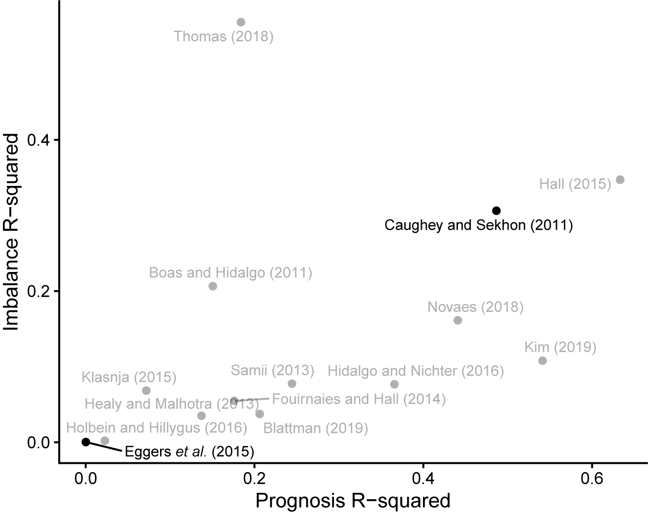


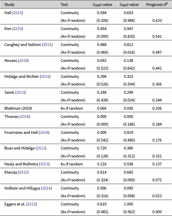


 Open access

