1. Introduction
When surface gravity waves propagate over an uneven seabed, wave–bottom interactions will occur. In a perturbation theory investigation of such interactions, Davies (Reference Davies1982) found resonant behaviour, which he termed Bragg resonance by analogy with the phenomenon of Bragg reflection originally identified in solid state physics by Bragg (Reference Bragg1914) during his investigation into the diffraction of X-rays by crystals. It was observed that crystals reflect X-rays most strongly when the crystal spacing is an integer multiple of half their wavelength. Davies’ discovery of Bragg resonance in wave–bottom interactions was the first appearance of this phenomenon in fluid mechanics, and it has subsequently been studied widely, owing to its practical applications in areas such as protection of coastlines and of offshore oil and gas production platforms against waves.
In the latter context, Mei, Hara & Naciri (Reference Mei, Hara and Naciri1988) proposed the use of an array of submerged artificial bars spaced such that Bragg resonance causes strong total reflection of primary transmitted waves, thus enabling the array to act as a breakwater. Several laboratory experiments and numerical simulations have been carried out to investigate such Bragg breakwaters, considering in particular the most efficient and cost-effective shapes and arrangements of the submerged bars (Davies & Heathershaw Reference Davies and Heathershaw1984; Guazzelli, Rey & Belzons Reference Guazzelli, Rey and Belzons1992; O’Hare & Davies Reference O’Hare and Davies1993; Cho et al. Reference Cho, Yoon, Lee and Yoon2001; Hsu, Tsai & Huang Reference Hsu, Tsai and Huang2003; Wang, Hsu & Chen Reference Wang, Hsu and Chen2006; Tsai et al. Reference Tsai, Kuo, Lan, Hsu and Chen2011; Liu, Shi & Cao Reference Liu, Shi and Cao2015). For example, among triangular, rectangular, trapezoidal and semicircular shapes, it has been found that the trapezoidal bars exhibited the best performance. In the particular case of dual composite artificial bars, Hsu et al. (Reference Hsu, Tsai and Huang2003) found that increasing the number of bars and their relative height can significantly strengthen the Bragg resonance effect, thereby effectively increasing the bandwidth over which the array exhibits high performance.
It has also been found that Bragg resonance can be exploited to focus wave energy. Zhang et al. (Reference Zhang, Tao, Tu, Su and Xie2021) employed the high-order spectral (HOS) method to investigate Bragg resonance in the case of regular and random waves propagating on an undulating bottom topography consisting of a horizontal V-shaped pattern. They found that within a certain range of values of the angle defining the V-shape, Bragg resonance leads to focusing of wave energy. Furthermore, Bragg resonance can also lead to an increase in the wave energy density and could thus be used to improve the efficiency of wave energy generation. Hao et al. (Reference Hao, Li, Liu and Wang2022) also used a numerical model based on the HOS method to investigate the effect of Bragg resonance on wave energy on a parabolic topography. Their results demonstrated that the wave focusing effect is markedly enhanced by increasing the ripple height, the number of ripples and the width of the topography. In addition, they found that the wave focusing is also influenced by the wave collection angle, and they determined an optimal range of this angle to provide the most effective focusing effect.
A number of studies have shown that when a wave system is subject to Bragg resonance, the angular frequencies of the wave components deviate from the resonance criterion established by Phillips (Reference Phillips1960) for interactions of surface waves, i.e. the Bragg resonance frequencies are downshifted or upshifted with respect to those predicted by this criterion. Liu & Yue (Reference Liu and Yue1998) compared the experimental results of Davies & Heathershaw (Reference Davies and Heathershaw1984) for surface wave propagation over a rippled bottom topography with the results of a perturbation theory analysis by Mei (Reference Mei1985) and the results of their own analysis based on the HOS method. They noted that the experimentally observed peak of the Bragg resonance did not occur at the point where the topographic ripple wavelength was half that of the surface waves, as predicted by perturbation theory, but instead there was a downshift of the resonant frequency (which was also predicted by the HOS analysis). A downshift was also found by Liu, Liu & Lin (Reference Liu, Liu and Lin2019b ) in their numerical study of steep waves on a corrugated reef based on a shock-capturing Boussinesq model. Furthermore, using the nonlinear shallow-water wave equations and Bloch energy band theory, Liu et al. (Reference Liu, Liu and Lin2019a ) found a similar resonant frequency downshift in the case of long-wave propagation on parabolic and rectified cosine bar arrays. They also found that the amount of downshift increased with increasing dimensionless height or width of the bars. Subsequently, Guo, Liu & Pan (Reference Guo, Liu and Pan2021) considered wave propagation over an array of finite-length cycloid-shaped bars or trenches, and to describe the reflection of waves by such an array, they derived an analytical solution of the modified mild-slope equation in the form of a Frobenius series. Their results confirmed the existence of the downshift in the Bragg resonant frequency in the case of cycloid-shaped bars, and also indicated that back reflection from cycloid-shaped trenches led to an upshift in the resonant frequency. Additionally, they found that these frequency shifts became more pronounced with increasing height and depth of the cycloid-shaped bars and trenches, respectively. Xu, Zhang & Zhang (Reference Xu, Zhang and Zhang2021) employed the homotopy analysis method (HAM; see Liao Reference Liao2012) to study Bragg resonances of strongly nonlinear waves over an undulating seabed, and their results again revealed the existence of the frequency upshift and downshift phenomena. Furthermore, they showed that an increase in the primary transmitted wave steepness led to an increase in the frequency shift.
Most of the above-mentioned studies of Bragg resonance concerned unsteady wave systems, although wave resonances can also occur in steady-state wave systems (Xu Reference Xu2014). Here, a wave system is classified as unsteady-state or steady-state according to whether or not its amplitude and frequency vary with time. Although most wave systems in nature are non-stationary, and steady-state wave systems occur less frequently, the study of the latter systems is crucial for our in-depth understanding of wave resonance. There have been many studies of steady-state wave systems (Xu et al. Reference Xu, Lin, Liao and Stiassnie2012, Reference Xu, Lin and Liao2015; Liu, Xu & Liao Reference Liu, Xu and Liao2017, Reference Xie, Ma, Dong and Perlin2021, Reference Xu, Zhao, Song and Zhang2023), and in particular, the HAM has been applied to investigate many aspects of such systems. Liao (Reference Liao2011) used the HAM to reveal that multiple exactly resonant steady-state wave systems can exist in deep water. Liao, Xu & Stiassnie (Reference Liao, Xu and Stiassnie2016) considered four-wave quasi-resonance. The nearly resonant wave problem was mathematically transformed into an exactly resonant one. It was found that from both physical and numerical viewpoints, the exact and near (quasi)-resonant waves exhibited no fundamental differences. Both problems were based on the resonance condition deduced by Phillips (Reference Phillips1960). Subsequently, Liu, Xu & Liao (Reference Liu, Xu and Liao2018) and Liu & Xie (Reference Liu and Xie2019) extended the work of Liao et al. (Reference Liao, Xu and Stiassnie2016) from the case of a single approximate resonance to multiple approximate resonances, and obtained steady-state wave groups of finite amplitude at infinite and finite water depths, respectively. In their study, Xie et al. (Reference Xie, Ma, Dong and Perlin2021) examined the resonant interactions of two gravity wave trains in deep water, and investigated how the steepness of the primary waves affected the evolution of the tertiary resonant wave, the three-dimensional wave patterns and the velocity profiles. Yang, Yang & Liu (Reference Yang, Yang and Liu2022) investigated steady-state exactly resonant waves, approximately resonant waves and non-resonant waves at infinite water depth. They found that in the case of exact third-order resonance, the energy in each wave system is mainly concentrated in the first- and third-order wave components. With increasing deviation from exact resonance, the energy in each wave system is gradually shifted to more wave components.
As noted previously, the study of steady-state wave systems is of great significance for our understanding of wave resonances. Such systems have been found for both exact and near resonances when waves propagate on periodically undulated beds that are infinite in extent. The corresponding problems have been claimed as class I and class II Bragg resonances (Xu et al. Reference Xu, Zhang and Zhang2021, Reference Xu, Zhao, Song and Zhang2023). However, the phenomenon studied by Xu et al. (Reference Xu, Zhang and Zhang2021, Reference Xu, Zhao, Song and Zhang2023) is actually not the Bragg resonance, but rather the water wave Bloch problem (McIver Reference McIver2000). Porter & Porter (Reference Porter and Porter2003) studied wave–structure interactions, including the scattering of waves by a finite section of periodic topography, the Bloch problem for infinite periodic topography and sloshing motions over periodic topography confined between vertical boundaries. Bragg scattering and the Bloch problem differ in three aspects. First, they differ in their mathematical nature: Bragg resonance is a boundary value problem, whereas the modulation of Bloch waves is an eigenvalue problem. Second, Bragg resonances are excited by a finite periodic undulating bottom, whereas Bloch waves are modulated by an infinite periodic undulating bottom. Third, in the Bragg resonance problem, owing to the finite extent of the periodic undulating bottom, lateral boundary conditions or radiation conditions at infinity need to be imposed, whereas for Bloch waves, owing to the infinite extent of the periodic undulating bottom, lateral boundary conditions or radiation conditions are not required. However, the two problems do share something in common: in both of these cases of resonances in wave propagation over a periodic bed, the corresponding resonance conditions (called Bragg’s law) can be borrowed from those derived by Phillips (Reference Phillips1960) for resonances in surface gravity waves.
The present paper considers the water wave Bloch problem in which a primary transmitted wave
 $\boldsymbol {k}_1$
passes over an undulating bottom modelled as a spatially infinite and stationary topography constructed from two waveforms with different wavenumbers
 $\boldsymbol {k}_{{b}i}$
(
 $i =1, 2$
) positioned at an angle to each other. It should be noted that for Bragg wave scattering by a finite undulating bottom, the wave coming from the front of the undulating bottom is called the incident wave. However, in this paper, since waves propagate over an infinite periodic bottom, it is not appropriate to call the surface wave
 $\boldsymbol {k}_1$
the incident wave. Instead, because the angle between
 $\boldsymbol {k}_1$
and
 $\boldsymbol {k}_{{b}1}+\boldsymbol {k}_{{b}2}$
is less than
 $90^\circ$
, we refer to it as the primary transmitted wave, with ‘primary’ meaning that the wave component is in the lowest order.
When resonance occurs, the following conditions are considered:
 \begin{gather} \boldsymbol {k}_1-\boldsymbol {k}_2-\boldsymbol {k}_{{b}1}-\boldsymbol {k}_{{b}2}=0, \end{gather}
 \begin{gather} \omega _1-\omega _2=\delta \omega , \end{gather}
where
 $\boldsymbol {k}_2$
is the wave vector of the resonant wave generated by the interactions between the primary transmitted wave and the topographic waveform,
 $\omega _1$
and
 $\omega _2$
are the angular frequencies of the transmitted and resonant waves, respectively, in linear theory, and
 $\delta \omega$
is the frequency detuning, which represents the difference between the frequency at which the approximate resonance occurs and that of the exact resonance. From the dispersion relation in finite water depth, it can be seen that the following relationship holds between the angular frequency and the wavenumber:
 \begin{equation} \omega _i^2=gk_i\tanh (k_id)\quad (i=1,2). \end{equation}
There is an important point that must be emphasised here. Physically, resonance refers to a situation in which a physical system vibrates with a greater amplitude at a specific frequency (called the resonant frequency) compared with other frequencies. When surface water waves interact with periodically undulating beds, resonance may occur at some specific frequency. In early studies, this resonant frequency was typically determined by Bragg’s law (Liu & Yue Reference Liu and Yue1998) in an approach borrowed from the mechanism of the nonlinear wave–wave interaction over a flat bottom derived by Phillips (Reference Phillips1960), in which one or more of the free-surface wave components in Phillips’ resonance conditions was replaced by periodic bottom components with zero frequencies. The corresponding resonance is called exact resonance (Liu Reference Liu2023). However, as mentioned by Liu (Reference Liu2023), Phillips’ condition was derived using a perturbative method, and the derivation did not take into account the effect of uneven beds. When the surface wave amplitude or the bottom irregularities increase, the wave slope grows or the relative amplitude of the bed is not small, Bragg’s law cannot accurately describe the corresponding resonance phenomenon. In other words, the resonant frequency determined by this condition is not truly the frequency corresponding to the actual resonance. There is a phase shift between these two frequencies (Linton Reference Linton2011; Liu Reference Liu2023; Fang, Tang & Lin Reference Fang, Tang and Lin2024). As pointed out by Linton (Reference Linton2011) and Ding, Liu & Lin (Reference Ding, Liu and Lin2024), the existence of this phase shift implies that Bragg’s law needs to be modified.
Therefore, in this paper, to investigate the resonance between surface waves and undulating beds of infinite extent on the basis of Phillips’ exact resonance condition, a small quantity
 $\delta \omega$
is introduced as a correction, as illustrated by (1.2). By varying the value of
 $\delta \omega$
, the energy of the resonant wave component and the equivalent wave steepness of the entire wave system are calculated to determine the frequency at which real resonance occurs. Owing to this frequency detuning, we refer to a resonance that satisfies the conditions (1.1) and (1.2) as near resonance. Adopting this approach, we can determine the actual resonant frequency that arises when waves interact with infinitely extended and undulating beds, and further study the characteristics of such Bloch wave systems at near resonance.
It should also be noted that the resonance between surface waves and the seabed is a complex phenomenon, influenced by various factors such as water depth, wave propagation angle and seabed topography. The mathematical principles underlying this phenomenon remain unclear (Liu Reference Liu2023). Understanding the resonance between different wave components is crucial, since it has an impact on the energy distribution within the entire wave system and thus affects the overall wave spectrum (Xie et al. Reference Xie, Ma, Dong and Perlin2021). It is essential to accurately identify the wave components involved in resonance, since even a slight deviation can lead to significant changes in the energy distribution across the entire wave system (Ding et al. Reference Ding, Liu and Lin2024).
The concept of near resonance is based on Phillips’ linear resonance condition. This paper aims to accurately determine the wavenumber and angular frequency of the wave component that truly resonates by introducing an appropriate frequency detuning
 $\delta \omega$
into this condition and adjusting its magnitude. This is crucial, because even slight deviations can cause significant changes in the steepness of the wave system, potentially hindering actual resonance. For example, as illustrated in figure 4(d), the detuning range corresponding to the steepness of the wave system is narrow. Therefore, straying from the detuning that matches the maximum steepness can lead to a rapid decrease in the steepness. Hence the primary objective of investigating near resonance is to accurately identify the wave system that actually resonates.
The steady-state Bloch wave systems are found using the HAM, and the energy distributions of the primary transmitted and resonant wave components, as well as the variations of the wave steepness and angular frequency of these wave systems, are investigated. Two subtypes (1 and 2) are found in these steady-state wave systems, of which subtype 1 has not previously been identified. The effect of the angle between the two components of the topographic waveform on the resonant wave systems is investigated, and it is found that the energy of the wave system increases significantly at specific values of this angle. Furthermore, it is found that variations in the parameters of the bottom topography lead to distribution of the energy of the wave system in more wave components.
The remainder of the paper is organised as follows. In § 2, the physical model employed in the study is described, and the mathematical formulation of the HAM framework is explained. In § 3, the results obtained for the Bloch wave systems are presented, and the effects of each physical parameter on the steady-state wave systems at near resonance are analysed. A detailed summary of the conclusions of the study is presented in § 4.
2. Definition of the wave system
2.1. Physical model
First, we establish a Cartesian coordinate system as illustrated in figure 1(a), where
 $(x, y)$
and
 $z$
denote the horizontal and vertical coordinates, respectively. The
 $x$
axis extends horizontally to the right, while the
 $z$
axis extends vertically upwards. The wave elevation is denoted by
 $\zeta (x,y,t)$
and represents the height of the free surface corresponding to
 $z = 0$
.
In this paper, we investigate the propagation of surface gravity waves over a periodically undulating bottom topography that extends infinitely in space and remains stationary. Two sets of undulations are superimposed on each other, as shown in the three-dimensional schematic in figure 1(b). The variable
 $z=-d+h_{1}(x,y)+h_{2}(x,y)$
represents the bottom undulation, where
 $h_{i}(x,y)=b_{i}\cos (\boldsymbol {k}_{{b}i}\boldsymbol {\cdot }\boldsymbol {r})$
 $(i=1,2)$
, with
 $\boldsymbol {r}=x\boldsymbol {i}+y\boldsymbol {j}$
. Here,
 $b_i$
and
 $\boldsymbol {k}_{{b}i}=\{k_{{b}i}\cos \theta _{i},k_{{b}i}\sin \theta _{i}\}$
are the amplitudes and wavenumbers of the bottom waveforms, with
 $\theta _{i}$
denoting the angle between
 $\boldsymbol {k}_{{b}i}$
and the
 $x$
axis;
 $\theta =\theta _{1}+\theta _{2}$
is the angle between
 $\boldsymbol {k}_{{b1}}$
and
 $\boldsymbol {k}_{{b2}}$
. The wavenumber of the primary transmitted wave is
 $\boldsymbol {k}_1=\{k_1\cos \alpha ,k_1\sin \alpha \}$
, where
 $k_1=|\boldsymbol {k}_1|$
, and
 $\alpha$
is the angle between
 $\boldsymbol {k}_1$
and the
 $x$
axis. The wave vector relationships at resonance are illustrated in figure 2.
(a) Schematic of the physical model of resonant Bloch waves propagating over a seabed. (b) Three-dimensional schematic of undulating bottom topography.

Plot of wave vector relations when resonance occurs.

2.2. Mathematical description
2.2.1. Governing equation and boundary conditions
The fluid is assumed to be homogeneous, inviscid and incompressible, and the flow is assumed to be irrotational. The wave system can be described in terms of a velocity potential
 $\varphi (x,y,z,t)$
, where
 $(x,y,z)$
are spatial variables and
 $t$
denotes time. The velocity potential
 $\varphi (x,y,z,t)$
satisfies the Laplace equation
 \begin{equation} \nabla ^2\varphi =0, \qquad -d+h_1(x,y)+h_2(x,y)\lt z\lt \zeta (x,y,t), \end{equation}
where
 \begin{equation} \nabla ^2=\frac {\partial ^2}{\partial x^2}+\frac {\partial ^2}{\partial y^2}+\frac {\partial ^2}{\partial z^2}. \end{equation}
The kinematic and dynamic boundary conditions at the free surface
 $z=\zeta (x,y,t)$
are
 \begin{gather} \zeta _t-\varphi _z+(\varphi _x\zeta _x+\varphi _y\zeta _y)=0, \end{gather}
 \begin{gather} g\zeta +\varphi _t+\tfrac {1}{2}\boldsymbol {\nabla }\varphi \boldsymbol {\cdot }\boldsymbol {\nabla }\varphi =0, \end{gather}
where
 $g$
is the gravitational acceleration. Taking time and space derivatives of (2.4) and combining the resulting equations with (2.3) enables us to eliminate
 $\zeta$
and obtain
 \begin{equation} \varphi _{tt}+g\varphi _z+2\boldsymbol {\nabla }\varphi \boldsymbol {\cdot }\boldsymbol {\nabla }\varphi _t+\tfrac 12\boldsymbol {\nabla }\varphi \boldsymbol {\cdot }\boldsymbol {\nabla }(\boldsymbol {\nabla }\varphi \boldsymbol {\cdot }\boldsymbol {\nabla }\varphi )=0. \end{equation}
In this paper, the bottom is taken to be stable and impermeable. The bottom boundary condition at
 $z=-d+h_1(x,y)+h_2(x,y)$
can be expressed as
 \begin{equation} \varphi _{z}=(h_{1x}+h_{2x})\varphi _{x}+(h_{1y}+h_{2y})\varphi _{y}. \end{equation}
To facilitate a dimensionless treatment of the governing equation and boundary conditions, we introduce dimensionless variables
 $X=k_{1x}$
,
 $Y=k_{1y}$
,
 $\Omega _{1}=\sigma _{1}/\omega _{1}$
,
 $T=\sigma _{1}t/\Omega _{1}$
and
 $Z=k_{1z}$
, where
 $\sigma _{1}$
is the actual frequency with nonlinear effects taken into account (see the dimensionless treatment in Xu et al. Reference Xu, Zhao, Song and Zhang2023). We define three phase functions
 $\xi _1$
,
 $\xi _2$
and
 $\xi _3$
as
 \begin{align} \xi _1=\boldsymbol {k}_1\boldsymbol {\cdot }\boldsymbol {r}-\sigma _1t=X\cos \alpha &+Y\sin \alpha -\Omega _1T, \end{align}
 \begin{align} \xi _2=\boldsymbol {k}_{{b}1}\boldsymbol {\cdot }\boldsymbol {r}=K_{{b1}}X\cos \theta _1&+K_{{b1}}Y\sin \theta _1, \end{align}
 \begin{align} \xi _3=\boldsymbol {k}_{{b}2}\boldsymbol {\cdot }\boldsymbol {r}=K_{{b2}}X\cos \theta _2&+K_{{b2}}Y\sin \theta _2. \end{align}
The governing equation and boundary conditions are rewritten in the following dimensionless forms, with
 $\xi _1$
,
 $\xi _2$
and
 $\xi _3$
serving as variables:
 \begin{align} &\qquad\qquad\quad\hat {\nabla }^2\phi =0, \quad -\varepsilon _1+\varepsilon _3\,H(\xi _2,\xi _3)\lt Z\lt \varepsilon _2\,\eta (\xi _1,\xi _2,\xi _3),&& \end{align}
 \begin{align} &\qquad\eta (\xi _1,\xi _2,\xi _3)=\tanh (\varepsilon _1)\,\Omega _1\phi _{\xi _1}-\varepsilon _2\tanh (\varepsilon _1)\,f, \quad Z=\varepsilon _2\,\eta (\xi _1,\xi _2,\xi _3), \end{align}
 \begin{align} &\Omega _1^2\phi _{\xi _1\xi _1}+\frac 1{\tanh (\varepsilon _1)}\,\phi _Z-2\varepsilon _2\Omega _1f_{\xi _1}+\varepsilon _2^2\,\hat {\boldsymbol {\nabla }}\phi \boldsymbol {\cdot }\hat {\boldsymbol {\nabla }}f=0, \quad Z=\varepsilon _2\,\eta (\xi _1,\xi _2,\xi _3), \end{align}
 \begin{align} &\qquad\qquad\quad\qquad\phi _Z-\varepsilon _3\,\hat {\boldsymbol {\nabla }}\phi \boldsymbol {\cdot }\hat {\boldsymbol {\nabla }}H=0, \quad Z=-\varepsilon _1+\varepsilon _3\,H(\xi _2,\xi _3), \end{align}
where
 \begin{align} H(\xi _2,\xi _3)={}&\cos (\xi _2)+\varepsilon _4\cos (\xi _3), \end{align}
 \begin{align} \hat {\boldsymbol {\nabla }}={}&\left (\cos \alpha\, \frac \partial {\partial \xi _1}+K_{{b1}}\cos \theta _1\,\frac \partial {\partial \xi _2}+K_{{b2}}\cos \theta _2\,\frac \partial {\partial \xi _3}\right )\boldsymbol {i}\nonumber \\ &{}+\left (\sin \alpha\, \frac \partial {\partial \xi _1}+K_{{b1}}\sin \theta _1\,\frac \partial {\partial \xi _2}+K_{{b2}}\sin \theta _2\,\frac \partial {\partial \xi _3}\right )\boldsymbol {j} +\left (\frac \partial {\partial z}\right )\boldsymbol {k}, \end{align}
 \begin{align} f={}&\tfrac 12(\phi _{\xi _1}^2+K_{{b1}}^2\phi _{\xi _2}^2+K_{{b2}}^2\phi _{\xi _3}^2+\phi _{Z}^2)+K_{{b1}}\cos (\alpha -\theta _1)\,\phi _{\xi _1}\phi _{\xi _2}\nonumber \\ &{}+K_{{b2}}\cos (\alpha -\theta _2)\,\phi _{\xi _1}\phi _{\xi _3}+K_{{b1}}K_{{b2}}\cos (\theta _1-\theta _2)\,\phi _{\xi _2}\phi _{\xi _3}. \end{align}
Here,
 $\varepsilon _{1}=k_{1}d$
,
 $\varepsilon _{2}=a_{1}k_{1}$
,
 $\varepsilon _{3}=b_{1}k_{1}$
and
 $\varepsilon _{4}=b_{2}/b_{1}$
are dimensionless parameters, and
 $a_1$
represents the measured (dimensional) wave amplitude of the primary transmitted wave with wavenumber
 $\boldsymbol {k}_1$
.
We apply the HAM to solve (2.10)–(2.13). The core principle of the HAM is to deform the unknown function from an initial guess to precise solutions through homotopy, achieved by introducing a physically meaningless embedding parameter. We first construct the zeroth-order deformation equations on the basis of the surface and bottom boundary conditions by introducing three mapping functions
 $\hat {\phi }(\xi _{1},\xi _{2},\xi _{3},Z;q)$
,
 $\hat {\eta }(\xi _1,\xi _2,\xi _3;q)$
and
 $\hat {\Omega }_1(q)$
. As
 $q$
changes from 0 to 1, the three mapping functions transition from their corresponding initial guesses to the precise solutions. A detailed explanation of the solution procedure can be found in Xu et al. (Reference Xu, Zhao, Song and Zhang2023).
2.2.2. Convergence verification
According to the convergence theorem of the HAM (Liao Reference Liao2012), three residual squares are defined as follows:
 \begin{align} \varepsilon _M^\phi &=\frac {1}{{\unicode[Arial]{x03C0}} ^3}\int _0^{{\unicode[Arial]{x03C0}} }\int _0^{{\unicode[Arial]{x03C0}} }\int _0^{{\unicode[Arial]{x03C0}} }\left (\sum _{n=0}^M\Delta _n^\phi \right )^3\,\mathrm {d}\xi _1\,\mathrm {d}\xi _2\,\mathrm {d}\xi _3, \end{align}
 \begin{align} \varepsilon _M^\eta &=\frac {1}{{\unicode[Arial]{x03C0}} ^3}\int _0^{{\unicode[Arial]{x03C0}} }\int _0^{{\unicode[Arial]{x03C0}} }\int _0^{{\unicode[Arial]{x03C0}} }\left (\sum _{n=0}^M\Delta _n^\eta \right )^3\,\mathrm {d}\xi _1\,\mathrm {d}\xi _2\,\mathrm {d}\xi _3, \end{align}
 \begin{align} \varepsilon _M^b&=\frac {1}{{\unicode[Arial]{x03C0}} ^3}\int _0^{{\unicode[Arial]{x03C0}} }\int _0^{{\unicode[Arial]{x03C0}} }\int _0^{{\unicode[Arial]{x03C0}} }\left (\sum _{n=0}^M\Delta _n^b\right )^3\,\mathrm {d}\xi _1\,\mathrm {d}\xi _2\,\mathrm {d}\xi _3, \end{align}
where
 $M$
denotes the homotopy approximation order. The terms
 $\Delta _n^{\phi }$
,
 $\Delta _n^{\eta }$
and
 $\Delta _{n}^{b}$
arise in solving the high-order deformation equations, and this theorem provides us with a convenient way to check the convergence and accuracy of the homotopy-series solution. All of
 $\Delta _n^{\phi }$
,
 $\Delta _n^{\eta }$
and
 $\Delta _{n}^{b}$
are functions of the convergence control parameter. Specific expressions for
 $\Delta _n^{\phi }$
,
 $\Delta _n^{\eta }$
and
 $\Delta _{n}^{b}$
can be found in the appendix of Xu et al. (Reference Xu, Zhao, Song and Zhang2023).
Relationships between
 $c_0$
and residual squares for
 $k_{1}d=1.5$
,
 $a_{1}k_{1}=0.02$
,
 $b_{1}k_{1}=0.02$
,
 $b_{2} / b_{1}=0.5$
,
 $k_{{b1}} / k_{{b2}}=0.8$
,
 $\alpha =70^{\circ }$
,
 $\theta =0^{\circ }$
and
 $\delta \omega =-0.00001$
. (a–c) Relationships between
 $c_0$
and
 $\log _{10}\varepsilon _{M}^{b}$
,
 $\log _{10}\varepsilon _M^\phi$
and
 $\log _{10}\varepsilon _M^\eta$
, respectively: dash-double-dotted line, first-order approximation; dash-dotted line, third-order approximation; dotted line, fifth-order approximation; dashed line, seventh-order approximation; solid line, ninth-order approximation. (d) Variation of squared residuals with order
 $M$
: solid line,
 $\log _{10}\varepsilon _{M}^{b}$
; dash-dotted line,
 $\log _{10}\varepsilon _M^\phi$
; dotted line,
 $\log _{10}\varepsilon _M^\eta$
.

To illustrate the selection of the convergence parameter and the verification of the homogeneous approximate solution, we take the following case as an example:
 \begin{equation} \begin{gathered} k_{1}d = 1.5, \quad a_{1}k_{1} = 0.02, \quad b_{1}k_{1} = 0.02, \\ b_{2} / b_{1} = 0.5, \quad k_{{b1}} / k_{{b2}} = 0.8, \quad \alpha = 70^{\circ }, \\ \theta = 0^{\circ }, \quad \delta \omega = -0.00001. \end{gathered} \end{equation}
Figures 3(a–c) display the relationships between the convergence control parameter
 $c_0$
and the three residual squares. It is evident that the three average residuals exhibit their steepest decreases when
 $c_0=1.2$
. Therefore,
 $c_0=1.2$
is chosen for subsequent computations of the residual squares. As depicted in figure 3(d), the residual squares exhibit a monotonic decrease as the approximation order
 $M$
is increased. This reduction reaches a minimum of 11 orders of magnitude by the 20th order, indicating successful convergence of the approximate solution obtained at
 $c_0=1.2$
. All results presented in this paper meet the criteria for convergence: (i) the three residual squares decrease by at least five orders of magnitude; (ii) as the approximation order
 $M$
increases, the three residual squares maintain a downward trend; (iii) all three residual squares are less than
 $1\times 10^{-6}$
; (iv) all results in this paper retain at least five significant figures.
3. Analysis of results
Before proceeding with a detailed analysis of the results obtained, we need to establish some definitions of certain variables and concepts. Specifically, these are the energy
 $E$
of the wave system, the relative contribution
 $a_{i,{p},{q}}^{2}/\Pi$
of each wave component to the total energy, and the wave steepness
 $h_{{s}}$
of the wave system. The energy of the wave system is defined as
 \begin{equation} E=\tfrac {1}{2} g \rho \sum _{i=0}^{+\infty }\sum _{p=-\infty }^{+\infty }\sum _{q=-\infty }^{+\infty }a_{i,p,q}^{2}=\tfrac {1}{2} g \rho \Pi , \end{equation}
where
 \begin{equation} \Pi =\sum _{i=0}^{+\infty }\sum _{p=-\infty }^{+\infty } \sum _{q=-\infty }^{+\infty }a_{i,p,q}^{2}, \end{equation}
and
 $a_{i,p,q}$
denotes the dimensionless amplitude of the wave component
 $\cos (i\xi _1+p\xi _2+q\xi _3)$
. According to this definition,
 $a_{1,0,0}^{2}/\Pi$
and
 $a_{1,-1,-1}^{2}/\Pi$
represent the individual contributions of the primary transmitted and resonant components, respectively, to the total energy of the wave system. We denote the combined contribution of the primary transmitted and resonant components to the total energy by
 \begin{equation} \Sigma _1=a_{1,0,0}^2 / \Pi +a_{1,-1,-1}^2 / \Pi . \end{equation}
Furthermore, building on the work of Liu et al. (Reference Liu, Xu and Liao2018) and Xu et al. (Reference Xu, Zhang and Zhang2021, Reference Xu, Zhao, Song and Zhang2023), the wave steepness of the entire steady-state wave system
 $h_{{s}}$
is defined as
 \begin{equation} h_{{s}}=\tfrac {1}{2}k_{{d}}(\eta _{{max}}-\eta _{{min}}), \end{equation}
where
 $k_{{d}}$
is the wavenumber of the dominant component with the largest amplitude in the wave system, and
 $\eta _{{max}}$
and
 $\eta _{{min}}$
are the maximum and minimum wave elevations within one wave period.
In this section, we will examine the energy distribution of the steady-state Bloch wave system at near resonance, and the factors that affect the wave steepness of the system.
3.1. Classification of wave systems
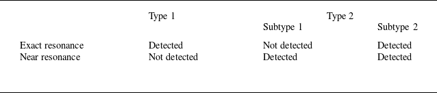
In previous studies of steady-state resonant Bloch waves, two types of waves, namely type 1 and type 2, have been identified on the basis of whether or not the energies of the primary transmitted and resonant wave components are the same throughout the entire steady-state wave system. In this paper, when resonance occurs and conditions (1.1) and (1.2) are satisfied, two subtypes within type 2, namely subtype 1 and subtype 2, are distinguished. These two subtypes possess distinct characteristics influenced by frequency detuning and bottom topography. The energy distribution and wave system steepness of subtype 1 vary monotonically with frequency detuning, whereas subtype 2 exhibits peaks in both the energy distribution and wave system steepness.
Table 1 presents a classification of steady-state waves at exact and near resonance. In a type 1 wave system, the primary transmitted and resonant components of the overall steady-state system have identical energy distributions, whereas in a type 2 wave system, they have distinct energy distributions.

It must be emphasised here that this study focuses exclusively on resonance phenomena in steady-state wave systems, which accordingly have amplitudes and frequencies that are independent of time. Put differently, once a designated set of parameters has been chosen for investigation, and the corresponding energy distribution of the wave system has been determined, the energy levels remain consistent throughout the wave’s duration. Any changes in energy levels discussed later in this paper are due to the use of a variety of physical parameter sets in the calculations.
3.2. Frequency detuning
The frequency detuning
 $\delta \omega$
given by (1.2) plays a crucial role in assessing proximity to resonance. To improve our understanding of wave system behaviour at near resonance, in this subsection, we will examine the influence of frequency detuning on a steady-state wave system at near resonance. Specifically, we will analyse the effects of frequency detuning on the energy distribution and wave steepness of the wave system, presenting a comparison between subtype 1 and 2 wave systems to highlight any distinct differences.
Influence of frequency detuning
 $\delta \omega$
on wave systems for
 $k_{1}d=1.5$
,
 $b_{1}k_{1}=0.07$
,
 $b_{2} / b_{1}=0.5$
,
 $a_{1}k_{1}=0.05$
,
 $\alpha =70^{\circ }$
,
 $k_{{b1}} / k_{{b2}}=0.8$
and
 $\theta =0^{\circ }$
. (a,b) Dependence of energy contributions (
 $a_{1,0,0}^{2} / \Pi$
,
 $a_{1,-1,-1}^{2} / \Pi$
) on
 $\delta \omega$
for subtype 1 and 2 wave systems, respectively. (c,d) Dependence of wave steepness
 $h_{{s}}$
on
 $\delta \omega$
for subtype 1 and 2 wave systems, respectively.

From figures 4(a,b), it is evident that in subtype 1, the energy ratio between the primary transmitted and resonant wave components follows a monotonic trend. Conversely, subtype 2 displays a peak rather than a monotonic variation. Specifically, in subtype 1, the energy contribution of the primary transmitted wave component,
 $a_{1,0,0}^{2}/\Pi$
, decreases gradually as the frequency detuning decreases, while that of the resonant wave component,
 $a_{1,-1,-1}^{2}/\Pi$
, increases gradually until it becomes the primary energy contributor to the entire wave system. Furthermore, with exact resonance (
 $\delta \omega =0$
, denoted by the green dot in figure 4
a) as the reference point, the energy disparity between the primary transmitted and resonant wave components increases proportionally to the frequency detuning
 $|\delta \omega |$
. In subtype 2, the energy contribution of the resonant wave component first increases and then decreases as the frequency detuning increases, reaching a peak at a certain point. Nonetheless, the energy contribution of the resonant wave component generally remains low. Note that at exact resonance, the energy ratios of the primary transmitted and resonant wave components in subtype 1 can be equal, whereas subtype 2 does not exhibit this equal distribution throughout the frequency range.
With regard to the effect of frequency detuning on the wave steepness, figures 4(c,d) illustrate the distinctions between the two subtypes of wave systems. In subtype 1, as the frequency detuning increases, there is a continuous decrease in wave steepness. Conversely, the wave steepness in subtype 2 exhibits a non-monotonic trend with increasing frequency detuning, peaking at a value
 $\delta \omega \gt 0$
rather than at
 $\delta \omega =0$
. Moreover, in subtype 2, as the primary transmitted wave steepness
 $a_1k_1$
increases, the peaks (represented by red dots in figure 4
d) in
 $h_{{s}}$
downshift further to positive values of
 $\delta \omega \gt 0$
. In previous studies, both upshifts and downshifts in frequency detuning were observed (Xu et al. Reference Xu, Zhang and Zhang2021). In the present study, a downshift in frequency detuning is also observed in subtype 2 systems.
Previous studies of resonant Bloch waves (Xu et al. Reference Xu, Zhang and Zhang2021, Reference Xu, Zhao, Song and Zhang2023) focused on examining the energy distribution of steady-state wave systems. However, in contrast to the present study, these only identified wave systems of subtype 2, and did not observe the existence of subtype 1, which is a key discovery presented here. The relationship between surface waves and bottom topography in the wave system described by subtype 1 satisfies the resonance conditions (1.1) and (1.2). However, within the range of
 $\delta \omega$
that we studied, there was no such case where a particular
 $\delta \omega$
corresponded to waves with maximum equivalent wave steepness. Meanwhile, the wave system’s equivalent wave steepness showed a monotonic change with
 $\delta \omega$
. If we base our understanding of resonance on the concept that resonance refers to a situation in which a physical system vibrates with greater amplitude at a specific frequency compared with other frequencies, then although subtype 1 satisfies the near-resonance condition, it cannot be considered as a resonant wave system. In other words, even within the frequency range determined by the near-resonance condition, non-resonant wave systems may exist. Previous research has focused more on the deviation between the actual resonant frequency and the frequency determined by precise resonance conditions, as shown by the properties of the wave system of subtype 2 in this study, which is based on the premise of resonance occurring. However, few studies have focused specifically on whether this premise always holds. The emergence of subtype 1 has brought new considerations and possibilities to the study of this issue, highlighting the importance of this type of wave system.
3.3. Impact of bottom topography
This subsection explores the influence of bottom topography on a steady-state wave system at near resonance, considering various parameters that characterise the bottom topography, namely the dimensionless amplitude
 $b_1k_1$
of the first of the two waveforms defining the bottom topography, the ratio
 $b_2/b_1$
of the amplitudes of the two waveforms, the angle
 $\theta$
between the two waveforms, and the propagation angle
 $\alpha$
of the primary wave.
3.3.1. Amplitudes of bottom waveforms
We first examine how
 $b_1k_1$
and
 $b_2/b_1$
affect the energy distribution in the resonant wave system. As shown in figures 5(a,c), in subtype 2, the energy contribution of the resonant wave increases with increasing
 $b_1k_1$
and
 $b_2/b_1$
, while that of the primary transmitted wave decreases. Changes in these parameters have less impact in subtype 1.
Influence of bottom topography on wave formation and propagation for
 $k_{1}d=1.5$
,
 $\alpha =70^{\circ }$
,
 $k_{{b1}} / k_{{b2}}=0.8$
,
 $\theta =0^{\circ }$
and
 $\delta \omega =-0. 0001$
. (a,b) Dependences of energy contributions of primary transmitted and resonant components (
 $a_{1,0,0}^{2} / \Pi$
,
 $a_{1,-1,-1}^{2} / \Pi$
) and combined energy contribution of primary transmitted and resonant components
 $\Sigma _{1}$
, respectively, on
 $b_{1}k_{1}$
for
 $a_{1}k_{1}=0.04$
and
 $b_{2} / b_{1}=0.5$
. (c,d) Dependences of energy contributions of primary transmitted and resonant components (
 $a_{1,0,0}^{2} / \Pi$
,
 $a_{1,-1,-1}^{2} / \Pi$
) and combined energy contribution of primary transmitted and resonant components
 $\Sigma _{1}$
, respectively, on
 $b_{2}/b_{1}$
for
 $a_{1}k_{1}=0.06$
and
 $b_{1}k_{1}=0.03$
.

The combined contribution of the primary transmitted and resonant wave components to the total energy is shown in figures 5(b,d). It is apparent that there is a significant decrease in
 $\Sigma _{1}$
with increasing
 $b_1k_1$
and
 $b_2/b_1$
, indicating that the influence of these wave components on the overall wave energy diminishes. As
 $b_1k_1$
and
 $b_2/b_1$
increase, the number of wave components in the system grows gradually, decreasing the percentage of primary transmitted and resonant wave energies, and this decrease is reflected in
 $\Sigma _{1}$
. A similar trend is observed as the angle between the topographic waveforms is varied, with more pronounced effects (see § 3.3.2). This is in agreement with the results of previous work on exact resonance by Xu et al. (Reference Xu, Zhao, Song and Zhang2023). Similar findings have also been reported by Xu & Liu (Reference Xu and Liu2020). All these studies highlight how multiple-wave nonlinear effects can introduce additional wave components, leading to a redistribution of energy within the wave system.
We now investigate how the values of
 $b_1k_1$
and
 $b_2/b_1$
affect the wave steepness
 $h_{{s}}$
and the dimensionless angular frequencies
 $\sigma _{1}/\omega _{1}$
and
 $\sigma _{2}/\omega _{2}$
of the primary transmitted and resonant waves in the wave system. The relationships between
 $b_1k_1$
and
 $b_2/b_1$
and the wave properties in the steady-state wave system are shown in figure 6. It can be seen that the wave properties are positively correlated with the variable parameters. Additionally, we see that the wave steepness and angular frequency in subtype 1 are higher than those in subtype 2, indicating differences between these two types of steady-state wave system. This is in agreement with the findings of Xu et al. (Reference Xu, Zhao, Song and Zhang2023) from their study of exact resonance. Overall, the influence of topographic waveform amplitude on wave steepness and angular frequency remains consistent and positively correlated, regardless of the type of resonance being considered.
Influence of bottom topography on wave systems for
 $k_{1}d=1.5$
,
 $\alpha =70^{\circ }$
,
 $k_{{b1}} / k_{{b2}}=0.8$
,
 $\theta =0^{\circ }$
and
 $\delta \omega =-0.0001$
. (a,b) Dependences of wave steepness
 $h_{{s}}$
and angular frequencies (
 $\sigma _{1}/\omega _{1}$
,
 $\sigma _{2}/\omega _{2}$
), respectively, on
 $b_1k_1$
for
 $a_{1}k_{1}=0.04$
and
 $b_{2} / b_{1}=0.5$
. (c,d) Dependences of wave steepness
 $h_{{s}}$
and angular frequencies (
 $\sigma _{1}/\omega _{1}$
,
 $\sigma _{2}/\omega _{2}$
), respectively, on
 $b_{2}/b_{1}$
for
 $a_{1}k_{1}=0.06$
and
 $b_{1}k_{1}=0.03$
.

3.3.2. Angle between topographic waveforms
One characteristic that distinguishes wave–bottom resonances is the number of waveforms in the undulating bottom topography. When the bottom consists of two waveforms, variations in the angle
 $\theta$
between these two waveforms will have an effect on the propagation of surface waves. However, to the best of our knowledge, previous studies have paid little attention to the influence of this angle on wave behaviour, and to remedy this defect, we examine this influence in detail. In particular, our present investigation has been prompted by the identification by Zhang et al. (Reference Zhang, Tao, Tu, Su and Xie2021) of a focusing effect at the bottom of the V shape formed between two topographic waveforms.
We consider angles in the range
 $\theta =0^{\circ }$
–
 $100^{\circ }$
. As we have seen from figures 5(b,d), when the two topographic waveforms are collinear (
 $\theta =0^{\circ }$
), the combined energy contribution of the primary transmitted and resonant wave components
 $\Sigma _{1}$
decreases with increasing
 $b_1k_1$
and
 $b_2/b_1$
. This indicates the presence of additional wave components in the system at larger values of
 $b_1k_1$
and
 $b_2/b_1$
. For example, in subtype 1, the combined energy contribution
 $\Sigma _{1}$
is
 $99.64\,\%$
at
 $b_1k_1=0.02$
, and decreases to
 $95.84\,\%$
at
 $b_1k_1=0.1$
(figure 5
b). It must be emphasised that the steady-state wave systems analysed in this study exhibit constant amplitudes and frequencies that remain consistent over time. This is similar to what was found in the study of the exact resonance by Xu et al. (Reference Xu, Zhao, Song and Zhang2023). Comparison of different wave systems with various values of physical parameters indicates the presence of additional wave components, beyond the resonant and primary transmitted components, and such a comparison enables us to identify which wave components contribute to the behaviour of these different steady-state wave systems.
As demonstrated in figure 7, variations in the angle
 $\theta \gt 0^{\circ }$
have significant effects on
 $\Sigma _{1}$
for both subtype 1 and subtype 2 wave systems. It can also be seen that these effects are more obvious as
 $b_2/b_1$
increases. This can be attributed to the presence of a greater number of wave components in the wave system when
 $\theta \gt 0^{\circ }$
, along with a greater energy contribution from components other than primary transmitted and resonant waves. It can be seen from figure 7 that the dependence of
 $\Sigma _{1}$
on
 $\theta$
differs between subtypes 1 and 2. First, in subtype 1,
 $\Sigma _{1}$
exhibits two local minima around
 $\theta =6^{\circ }$
and
 $40^{\circ }$
, respectively, whereas in subtype 2, there are two local minima around
 $\theta =14^{\circ }$
and
 $40^{\circ }$
. Second, the absolute minimum of
 $\Sigma _{1}$
in subtype 1 is approximately
 $91.38\,\%$
and corresponds to the local minimum at the lower value
 $\theta =6^{\circ }$
, whereas the absolute minimum of
 $\Sigma _{1}$
in subtype 2 is approximately
 $88.87\,\%$
and corresponds to the local minimum at the higher value
 $\theta =40^{\circ }$
. It is also noteworthy that in both subtypes, the values of
 $\theta$
corresponding to the local minima of
 $\Sigma _{1}$
remain consistently stable and do not change with variations in
 $b_2/b_1$
.
Influence of the angle
 $\theta$
between the waveforms of the bottom topography on the combined energy contribution of primary transmitted and resonant components
 $\Sigma _{1}$
for
 $k_{1}d=1.5$
,
 $a_{1}k_{1}=0.06$
,
 $b_{1}k_{1}=0.02$
,
 $k_{{b1}} / k_{{b2}}=0.8$
,
 $\alpha =78^{\circ }$
and
 $\delta \omega =0.00004$
: (a) subtype 1; (b) subtype 2.

Influence of the angle
 $\theta$
between the waveforms of the bottom topography in subtype 1 on the energy contribution of each wave component in the wave system for
 $k_{1}d=1.5$
,
 $a_{1}k_{1}=0.06$
,
 $b_{1}k_{1}=0.02$
,
 $b_{2} / b_{1}=1.0$
,
 $k_{{b1}} / k_{{b2}}=0.8$
,
 $\alpha =78^{\circ }$
and
 $\delta \omega =0.00004$
. (a) Energy contributions of all wave components. (b) Energy contributions of wave components other than primary transmitted and resonant waves.

Influence of the angle
 $\theta$
between the waveforms of the bottom topography in subtype 2 on the energy contribution of each wave component in the wave system for
 $k_{1}d=1.5$
,
 $a_{1}k_{1}=0.06$
,
 $b_{1}k_{1}=0.02$
,
 $b_{2} / b_{1}=1.0$
,
 $k_{{b1}} / k_{{b2}}=0.8$
,
 $\alpha =78^{\circ }$
and
 $\delta \omega =0.00004$
. (a) Energy contributions of all wave components. (b) Energy contributions of wave components other than primary transmitted and resonant waves.

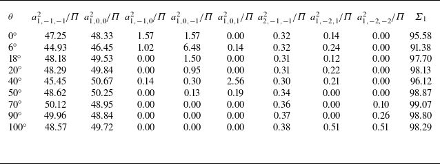
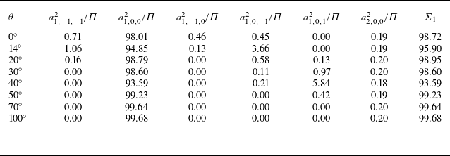
For a clearer understanding of the energy distribution in the wave system, all wave components in subtypes 1 and 2 with energy contributions exceeding
 $0.1\,\%$
have been identified and are presented in detail in figures 8 and 9, as well as in tables 2 and 3, from which it is evident that there is a pronounced increase in the energy contribution of the remaining wave components within the wave system for relatively low values of
 $\Sigma _{1}$
. This suggests that the energy of the wave system is distributed across a greater number of wave components, with some being allocated to higher-order components. Taking subtype 1 as an example, figures 8(b) and 9(b) demonstrate that the energy contributions of each of the wave components other than the resonant and primary transmitted wave components vary with the angle
 $\theta$
. Furthermore, the wave components that make the greatest contribution are not always the same. In particular, the component
 $\cos (\xi _{1}-\xi _{3})$
makes the greatest contribution in the vicinity of
 $\theta =6^{\circ }$
, whereas the component
 $\cos (\xi _{1}+\xi _{3})$
makes the greatest contribution in the vicinity of
 $\theta =40^{\circ }$
. This phenomenon occurs consistently in both subtype 1 and subtype 2.
Energy contribution (%) of each wave component in a steady-state wave system at near resonance for different angles
 $\theta$
between the waveforms of the bottom topography (subtype 1).

Energy contribution (%) of each wave component in a steady-state wave system at near resonance for different angles
 $\theta$
between the waveforms of the bottom topography (subtype 2).

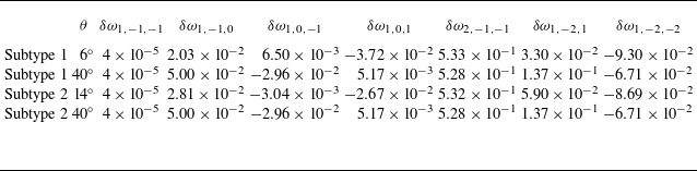
To explore the reason behind the energy distribution mentioned above, we substitute the wave components shown in figures 8 and 9 into the following general resonance conditions:
 \begin{gather} i\boldsymbol {k}_1 +p\boldsymbol {k}_{{b}1}+q\boldsymbol {k}_{{b}2}=\boldsymbol {k}_{i,p,q}, \end{gather}
 \begin{gather} \omega _1=\delta \omega _{i,p,q}+\omega _{i,p,q}. \end{gather}
We denote these conditions as
 $\mathrm {Res}(i,p,q)$
. Thus, for example,
 $\mathrm {Res}(1,-1,-1)$
corresponds to conditions (1.1) and (1.2). The corresponding
 $\delta \omega _{i,p,q}$
are listed in table 4. It can be seen that at the two peaks (
 $\theta =6^{\circ }$
and
 $40^{\circ }$
for subtype 1;
 $\theta =14^{\circ }$
and
 $40^{\circ }$
for subtype 2), the values of
 $\delta \omega _{i,p,q}$
for the wave components
 $\cos (\xi _1-\xi _3)$
and
 $\cos (\xi _1+\xi _3)$
, i.e.
 $\delta \omega _{1,0,-1}$
and
 $\delta \omega _{1,0,1}$
, are relatively small, indicating that near resonances also occur among these components, the primary transmitted wave
 $\cos (\xi _1)$
and the seabed. In other words, multiple resonances exist simultaneously. For example, in subtype 1, when
 $\theta =6^{\circ }$
, the near-resonance conditions
 $\mathrm {Res}(1,-1,-1)$
and
 $\mathrm {Res}(1,0,-1)$
are satisfied. Thus except for the component
 $\cos (\xi _1-\xi _2-\xi _3)$
, the energy of the component
 $\cos (\xi _1-\xi _3)$
cannot be ignored. The same phenomenon also occurs in the other three scenarios shown in table 4. As mentioned above, multiple resonances also occur among surface gravity waves propagating over a flat seabed (Liu et al. Reference Liu, Xu and Liao2018).


For further clarity, let us delve deeper into the occurrence of resonance and the wave components involved. For resonance to occur, there are two requirements: (i) the exact or near resonance conditions must be satisfied, and (ii) the corresponding resonant wave components must have a non-negligible amount of energy. The data on
 $\delta \omega$
in table 4 show that there are one or two wave components that meet both of these requirements, and their energy contribution is higher than that of other higher-order wave components. Taking subtype 1 as an example, at
 $\theta =6^{\circ }$
,
 $\delta \omega _{1,-1,-1}$
and
 $\delta \omega _{1,0,-1}$
are equal to
 $4\times 10^{-5}$
and
 $6.5\times 10^{-5}$
, respectively. Table 2 also presents the energy contributions of these two wave components in the entire wave system:
 $6.48\,\%$
and
 $44.93\,\%$
, respectively. This indicates that
 $\cos (\xi _1-\xi _2-\xi _3)$
and
 $\cos (\xi _1-\xi _3)$
are both resonant wave components. For subtype 2, at
 $\theta =40^{\circ }$
,
 $\delta \omega _{1,-1,-1}$
and
 $\delta \omega _{1,0,1}$
are equal to
 $4\times 10^{-5}$
and
 $5.17\times 10^{-3}$
, respectively, while the energy contributions of these two wave components are 0 and
 $5.84\,\%$
, respectively. This allows us to confirm that resonance does indeed occur, and the resonant component is
 $\cos (\xi _1+\xi _3)$
. In the cases shown in figures 8 and 9, in addition to the resonance components, there are actually other high-order wave components involved in the interaction. For example, in the case
 $\theta =6^{\circ }$
in subtype 1, apart from
 $\cos (\xi _1-\xi _2-\xi _3)$
and
 $\cos (\xi _1-\xi _3)$
, the energies of
 $\cos (\xi _1-\xi _2)$
,
 $\cos (\xi _1+\xi _3)$
,
 $\cos (2\xi _1-\xi _2-\xi _3)$
and
 $\cos (\xi _1-2\xi _2-\xi _3)$
also account for a certain proportion. In fact, wave components of even higher orders are present, but their energy is much smaller. It should be noted that the number of wave components involved in the interaction increases with increasing wave steepness. Usually, as the steepness of the waves increases, higher-order wave components involved in the nonlinear interaction will make a more substantial energy contribution, thus a greater number of wave components will participate in the interaction. It is worth noting that this conclusion has been corroborated in the case of waves propagating in deep water with multiple near resonances occurring (Liu et al. Reference Liu, Xu and Liao2018).
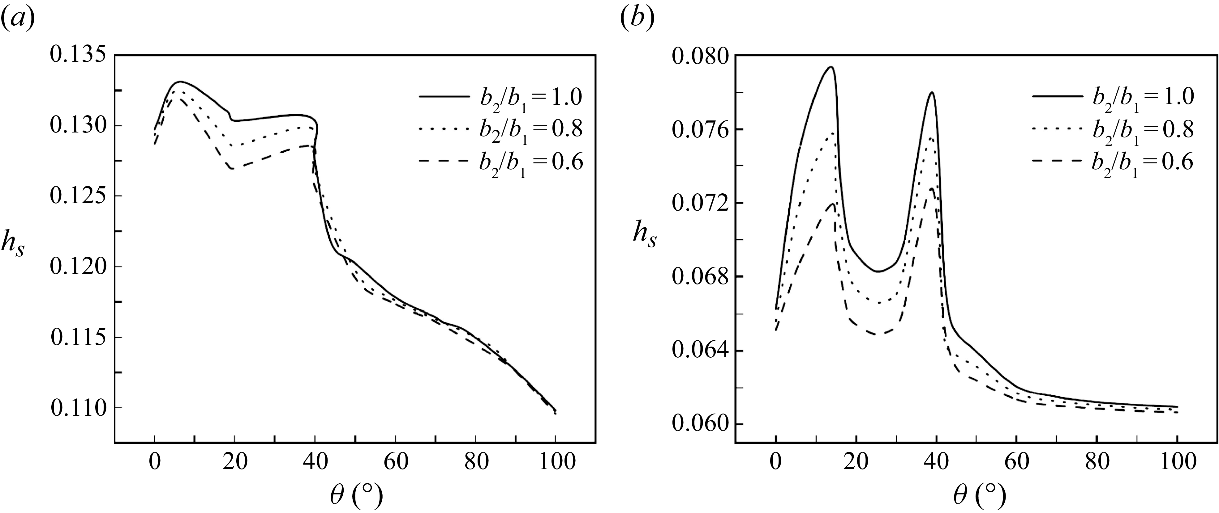
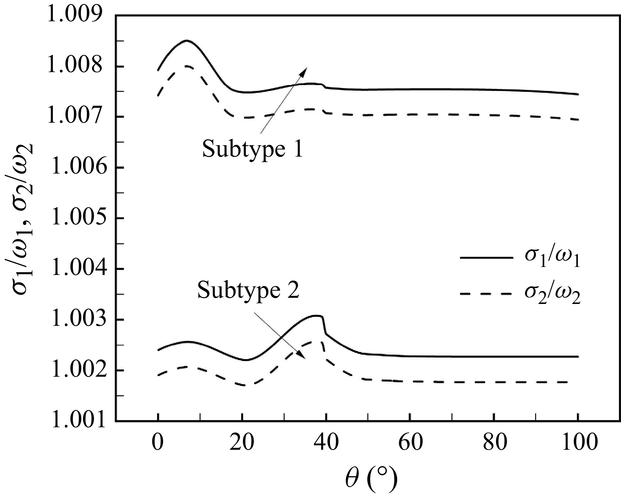
Further investigations reveal that the angle
 $\theta$
also has a significant influence on wave steepness and angular frequency, as illustrated in figures 10–12. It can be seen that both the wave steepness and angular frequency exhibit pairs of peaks, and that these occur at the same angles as the local minima in the combined energy contribution of the primary transmitted and resonant components
 $\Sigma _{1}$
. Furthermore, we also find that in subtype 2, for
 $\theta \gt 50^{\circ }$
, the wave steepness
 $h_{{s}}$
is almost unaffected by changes in
 $\theta$
. This is in contrast to subtype 1, where
 $h_{{s}}$
exhibits a continuously decreasing trend for
 $\theta \gt 40^{\circ }$
. Moreover, in both subtypes, the steepness of the wave system for
 $\theta \gt 50^{\circ }$
is smaller than for
 $\theta =0^{\circ }$
. In this angular range, changes in
 $b_{2}/b_{1}$
and
 $k_{{b1}}/k_{{b2}}$
have a more limited effect on the wave system than in the small-angle case. However, increasing
 $k_{{b1}}/k_{{b2}}$
in subtype 1 does not necessarily increase the wave steepness of the wave system, but actually decreases it at some angles.
In addition, we examine the influence of various parameters on the peak values, namely the ratios
 $b_2/b_1$
and
 $k_{{b1}}/k_{{b2}}$
, and the propagation angle
 $\alpha$
of the primary transmitted wave component. The peaks are not affected at all by
 $b_2/b_1$
(see figure 10), but are slightly affected by
 $k_{{b1}}/k_{{b2}}$
(see figure 11) and significantly affected by
 $\alpha$
(see figure 13). In particular, as shown in figure 13, we examine the wave steepness of the whole wave system for different values of
 $\alpha$
. When
 $\alpha$
varies from
 $70^{\circ }$
to
 $78^{\circ }$
, both the numbers of the peaks and their values change. It should be noted that the ratio
 $b_2/b_1$
does not appear in the resonance conditions (1.1) and (1.2). Its value does not affect the magnitude and direction of the wave components that participate in the resonance. However, changes in
 $k_{{b1}}/k_{{b2}}$
and
 $\alpha$
will directly affect those wave components, and further change the wave systems. Thus both of them will affect the peaks, but the impact of
 $\alpha$
is more significant.
Influence of the angle
 $\theta$
between the waveforms of the bottom topography on the wave steepness
 $h_{{s}}$
of the wave system for
 $k_{1}d=1.5$
,
 $a_{1}k_{1}=0.06$
,
 $b_{1}k_{1}=0.02$
,
 $k_{{b1}} / k_{{b2}}=0.8$
,
 $\alpha =78^{\circ }$
and
 $\delta \omega =0.00004$
, and different values of
 $b_2/b_1$
: (a) subtype 1; (b) subtype 2.

Influence of the angle
 $\theta$
between the waveforms of the bottom topography on the wave steepness
 $h_{{s}}$
of the wave system for
 $k_{1}d=1.5$
,
 $a_{1}k_{1}=0.06$
,
 $b_{1}k_{1}=0.02$
,
 $b_2 / b_1=0.5$
,
 $\alpha =78^{\circ }$
and
 $\delta \omega =0.00004$
, and different values of
 $k_{{b1}}/k_{{b2}}$
: (a) subtype 1; (b) subtype 2.

Influence of the angle
 $\theta$
between the waveforms of the bottom topography on the angular frequencies (
 $\sigma _{1}/\omega _{1}$
,
 $\sigma _{2}/\omega _{2}$
) of subtype 1 and subtype 2 wave systems for
 $k_{1}d=1.5$
,
 $a_{1}k_{1}=0.06$
,
 $b_{1}k_{1}=0.02$
,
 $b_{2} / b_{1}=1.0$
,
 $k_{{b1}} / k_{{b2}}=0.8$
,
 $\alpha =78^{\circ }$
and
 $\delta \omega =-0.0005$
.

Influence of the angle
 $\theta$
between the waveforms of the bottom topography on the wave steepness
 $h_{{s}}$
of the wave system for
 $k_{1}d=1.5$
,
 $a_{1}k_{1}=0.06$
,
 $b_{1}k_{1}=0.02$
,
 $b_2 / b_1=0.5$
,
 $k_{{b1}}/k_{{b2}}=0.8$
and
 $\delta \omega =0.00004$
and different values of
 $\alpha$
: (a) subtype 1; (b) subtype 2.

It is important to note that according to the definition (3.4) of the wave steepness
 $h_{{s}}$
adopted in this paper, and the assumption that wave energy is directly proportional to wave amplitude, the magnitude of
 $h_{{s}}$
provides some indication of the total energy of the wave system. It should also be noted that primary conversion of wave energy is attained by an oscillating system, and this is able to store some kinetic and/or potential energy (Brooke Reference Brooke2003). Most wave energy converters (WECs) are oscillating-body devices (Falcao Reference Falcao2010). Since energy production by oscillating bodies is governed by wave-induced motion, the dimensions of such WECs are constrained significantly by the incident wavelengths.
The design of a WEC typically involves consideration of the local primary wave frequencies. When the natural frequency of the WEC is close to the primary local wave frequency, resonance occurs between the WEC and the waves, resulting in significant relative motion between the two. The WEC then converts this mechanical energy into electricity (Xu, Stuhlmeier & Stiassnie Reference Xu, Stuhlmeier and Stiassnie2018). On the other hand, according to the wave–bottom resonance studied in this paper, and depending on the local primary wave frequency, the seabed topography can be adjusted and designed to enhance the wave amplitude after resonance with the surface waves, thereby allowing the WEC to undergo greater relative motion and capture more wave energy. Thus wave–bottom resonance can be exploited to design the appropriate seabed topography for a given marine area, and determine the geometrical parameters of a WEC wave energy harvesting device so that it captures as much wave energy as possible.
In this paper, a dual-frequency seabed topography has been considered, and for certain specific angles, the studied steady-state resonant wave system exhibits a larger amplitude. Thus the use of wave energy collection devices based on bottom topographies characterised by angles
 $\theta$
corresponding to the peak values of
 $h_{{s}}$
revealed in the above analysis should help to maximise the amount of wave energy that can be harvested. Such an approach to improving the effectiveness of wave energy harvesting closely resembles the approaches of Zhang et al. (Reference Zhang, Tao, Tu, Su and Xie2021) and Hao et al. (Reference Hao, Li, Liu and Wang2022).
4. Conclusions and discussion
This study has thoroughly explored steady-state wave systems at near resonance using the homotopy analysis method, focusing on the occurrence of resonance when a primary transmitted surface wave passes over an undulating bottom modelled as a spatially infinite and stationary topography constructed from two waveforms with different wavenumbers positioned at an angle to each other. The effects of different physical parameters on the energy distribution, wave steepness and angular frequencies of both the primary transmitted and resonant wave components of a stationary wave system have been examined.
Previous studies have categorised steady-state wave systems at wave–bottom resonance as either type 1 or type 2, depending on whether or not the energy distributions in the primary transmitted and resonant wave components are the same. The present study has introduced two subtypes of type 2 steady-state wave systems at near resonance: subtype 1 and subtype 2. Subtype 1 is exclusive to steady-state wave systems, representing a previously unidentified and distinctive subgroup characterised by monotonic variations in both energy distribution and wave steepness in response to frequency detuning. On the other hand, subtype 2 exhibits varying wave steepness in a wave system with frequency detuning
 $\delta \omega$
, displaying a distinct peak in the range
 $\delta \omega \gt 0$
. This peak shifts to more positive values of
 $\delta \omega$
as the primary transmitted wave steepness increases, in what is known as a downward shift of the resonant frequency. This phenomenon, which was also observed by Xu et al. (Reference Xu, Zhang and Zhang2021), further emphasises the distinctive characteristics of subtype 2.
The influences on the wave system of the dimensionless amplitude
 $b_1k_1$
of the first of the two topographic waveforms, and the ratio
 $b_2/b_1$
of the amplitudes of the two topographic waveforms, have also been investigated. Xu et al. (Reference Xu, Zhao, Song and Zhang2023) noted that with increasing
 $b_1k_1$
and
 $b_2/b_1$
, additional wave components emerge within the wave system, contributing to the distribution of energy. A similar trend has been observed in this study. In addition, a positive correlation has been found between
 $b_1k_1$
,
 $b_2/b_1$
, the wave steepness
 $h_{{s}}$
of the wave system, and the angular frequencies of both resonating and primary transmitted waves. These findings are consistent with results reported by Xu et al. (Reference Xu, Zhao, Song and Zhang2023) for exact resonance.
Furthermore, a detailed analysis has been presented here of the influence on the wave system of the angle
 $\theta$
between the two topographic waveforms (ranging from
 $0^\circ$
to
 $100^\circ$
). When
 $\theta \gt 0$
, other wave components in addition to the primary transmitted and resonant waves will contribute to the total energy of the steady-state wave system. For example, in subtype 1 when
 $\alpha =78^{\circ }$
, the sum of the energy contributions of the primary transmitted and resonant waves
 $\Sigma _{1}$
is approximately
 $91.38\,\%$
at
 $\theta =6^\circ$
, but it is reduced to
 $88.87\,\%$
at
 $\theta \approx 40^\circ$
in subtype 2. This value is significantly lower than what is observed when the topographic waveforms are collinear (i.e.
 $\theta =0^\circ$
).
It has been demonstrated that the wave system exhibits a pair of peaks in the angular range
 $\theta \in [0^\circ , 100^\circ ]$
. The values of the peaks are not affected by the amplitude ratio of the bottom waveforms
 $b_2/b_1$
, but are slightly affected by the wavenumber ratio of the waveforms
 $k_{{b}1}/k_{{b}2}$
, and significantly affected by the propagation angle
 $\alpha$
of the primary transmitted wave
The wave steepness
 $h_{{s}}$
as defined in this study serves as an indicator of the energy within a wave system. An analysis of the influence of
 $\theta$
on
 $h_{{s}}$
has shown that wave systems tend to exhibit higher energy levels at specific angles. Therefore, by leveraging this characteristic, adjustments to the bottom topography can be used to enhance the energy of a wave system and thereby improve the effectiveness of wave energy harvesting devices.
The influence of
 $\theta$
on the angular frequencies of the primary transmitted and resonant wave components resembles that on the wave steepness. As
 $\theta$
varies, the angular frequencies exhibit pairs of primary and secondary peaks. When
 $b_2/b_1=0.06$
, the positions of the primary and secondary peaks in subtypes 1 and 2 are opposite to each other, but apart from this, the positions of the primary and secondary peaks in both types of wave systems remain unchanged. However, in both subtypes, when
 $\theta \gt 40^\circ$
, the angular frequencies do not change significantly with increasing
 $\theta$
.
Furthermore, it should be noted that as mentioned by Porter & Porter (Reference Porter and Porter2003) and Linton (Reference Linton2011), the Bragg resonance band and the Bloch stop band are closely related. Porter & Porter (Reference Porter and Porter2003) studied the scattering of waves by a finite section of periodic seabed and the Bloch problem for infinite periodic topography. They concluded that the frequency bands supporting the existence of Bragg resonance in the scattering problem corresponded to the non-existence of propagating Bloch waves. Linton (Reference Linton2011) investigated water waves propagating over infinite periodic arrays of submerged horizontal circular cylinders in deep water, and established the existence of a band-gap structure. The numerical results showed that band gaps do exist. Meanwhile, the energy transmitted across a finite array tends to zero as the size of the array increases. In this paper, we have aimed to find the accurate frequency of the Bloch wave at resonance. However, this does not mean that only resonant waves, but no transmitted waves, can exist in such wave systems. The corresponding resonant frequency seems not to correspond to the stop band defined by Linton (Reference Linton2011). At the frequencies considered in this paper, transmitted and resonant waves coexist, and therefore, rather than transmitted waves being impossible or tending to zero, they may contribute a relatively large proportion of the energy of the entire wave system. In fact, the present study is closer to the work of Fang et al. (Reference Fang, Tang and Lin2024), in that both consider the resonant frequency as well as the deviation between this frequency and the frequency determined by Bragg’s law derived under linear conditions. However, Fang et al. (Reference Fang, Tang and Lin2024) consider Bragg resonance under the interaction of bottom terrain and surface waves in a limited area, whereas this paper considers Bloch wave–bottom resonance in the interaction between surface waves and bottom terrains of infinite extent.
Although this paper has presented a thorough theoretical analysis of the behaviour of a steady-state wave system at near resonance, and the factors influencing this behaviour, there is scope for much future work in this area along a number of directions.
-
(i) There is currently a lack of any experimental validation of the theoretical results obtained here. Therefore, experiments need to be planned and conducted to obtain suitable data to provide such validation.
-
(ii) It is known that Bragg resonance can be categorised into four classes (I, II, III and IV) on the basis of the number of surface waves and topographic waveforms involved in the resonance. A similar categorisation applies to the corresponding Bloch wave problem. Previous studies have identified steady-state wave systems for Bloch waves at exact and near resonances when the topography involves one or two waveforms and the surface waves have only one primary transmitted wave. We hypothesize that steady-state wave systems may also exist when resonances occur among multiple surface waves and topographic waveforms. Therefore, future research on steady-state wave systems should extend to include these cases.
-
(iii) It has been found in this study that for specific values of the angle between the two waveforms defining the bottom topography, the energy of the wave system is significantly increased. Thus with an appropriate arrangement of the bottom topography, the wave energy density in a specific area can be substantially increased, and the effectiveness of wave energy harvesting devices can be improved. This is of great significance for the development and utilisation of wave energy. Therefore, we recommend that future research should further explore the role of wave–bottom resonance in wave energy concentration.
Acknowledgements.
Thanks go to the anonymous reviewers for their valuable comments and suggestions that have enhanced the quality of this paper.
Funding.
This work was supported by the National Natural Science Foundation of China (grant nos 11602136 and 51679132) and the Shanghai Frontiers Science Center of Full Penetration Far-Reaching Offshore Ocean Energy and Power.
Declaration of interests.
The authors report no conflict of interest.
Author contributions.
D.X.: conceptualisation (lead); formal analysis (equal); funding acquisition (lead); investigation (lead); methodology (lead); supervision (lead); writing – review and editing (lead). H.L.: data curation (equal); formal analysis (equal); investigation (equal); writing – original draft (equal). H.Z.: funding acquisition (supporting); writing – review and editing (supporting).
Data availability statement.
The data that support the findings of this study are available from the corresponding author upon reasonable request.