

Implications
Farm-scale models can be used to document greenhouse gas (GHG) emissions and predict the likely consequences of mitigation measures on both emissions and production. However, regulators and commercial organisations need assurance of the validity of their use. An inter-comparison of models should form part of this process.
Introduction
Globally, the livestock sector accounts for 14.5% of human-caused GHG emissions, producing 7.1 Gt of carbon dioxide equivalent (CO2e) emissions per year, of which dairy farming contributes about 20% (Hagemann et al., Reference Hagemann, Ndambi, Hemme and Latacz-Lohmann2012). European dairy production is over 150 million tonnes of milk and accounts for about 15% of the value of all European agricultural production (European Commission, 2017). However, it also accounts for about one-third of GHG emissions from the European livestock sector (Bellarby et al., Reference Bellarby, Tirado, Leip, Weiss, Lesschen and Smith2013). The sources of direct on-farm GHG emissions are methane (CH4) from enteric fermentation and manure management, and nitrous oxide (N2O) from manure management and the soil. In addition, there are indirect GHG emissions in the form of N2O, resulting from the nitrification and partial denitrification of reduced forms of nitrogen (N) that occur off-farm, either as a result of the atmospheric deposition of N from ammonia (NH3) volatilization from on-farm manure management and the soil, or from nitrate (NO3 −) leaching from the fields on the farm (IPCC, 2006). Finally, changes to the amount of C stored in the soil can act as a source or sink for CO2.
Hitherto, there has been limited regulatory pressure to reduce GHG emissions from agriculture, although there is increased interest from the food retail sector concerning their GHG emissions and that of their supply chains (e.g. Tesco PLC, 2016). However, the European Union (EU) is currently in the process of supplementing its Effort Sharing Decision (European Commission, 2009) with an Effort Sharing Regulation (ESR; Erbach, Reference Erbach2016) that by 2030 compared with 2005, will reduce by 30% the GHG emissions from the sectors not included in the European Emissions Trading Scheme (agriculture, transport, buildings, small industry and waste). The agreement will place a heavier burden on the wealthier Member States and impose national Annual Emission Allocations but will allow some flexibility concerning the distribution of reduction burden between sectors and allow limited transfer or trading of Annual Emission Allocations. How the ESR will be implemented in individual Member States is unclear, including the proportion of the emission reduction allocated to agriculture and the extent to which there is the ability and willingness to utilise the flexibility mechanisms. However, as the ESR contains reduction targets for EU member states that range from 0% to 40%, significant reductions seem likely to be demanded from agriculture, especially for more wealthy Member States with large agricultural sectors. Member States that decide they need to reduce agricultural GHG emissions will need to choose a method of implementing reduction measures and how these will be documented in their national GHG inventories. This could include devolving the choice of measures and GHG accounting to individual farms, and the use of farm typologies in their national GHG accounting.
Ruminant livestock farms in general, and dairy cattle farms in particular, typically rely heavily on on-farm crop production to supply animal feed. This leads to a substantial internal cycling of nutrients (Jarvis et al., Reference Jarvis, Hutchings, Brentrup, Olesen and van der Hoek2011), feedback effects between farm components (livestock, manure management, etc.), and difficulty in obtaining the information concerning feed intake necessary to calculate the major sources of GHG emissions using the Tier 2 IPCC methodology. Member States will need to assess the cost and effectiveness of the mitigation measures needed to achieve the ESR reductions and report projected emissions (European Commission, 2013). As noted by Crosson et al. (Reference Crosson, Shalloo, O’Brien, Lanigan, Foley, Boland and Kenny2011), whole-farm systems models offer a more consistent approach than IPCC methodologies when assessing GHG emissions from such farms. This includes capturing feedback effects and allowing the consequences of mitigation measures on production and costs to be assessed.
A number of whole-farm cattle systems models have been developed (Del Prado et al., Reference Del Prado, Crosson, Olesen and Rotz2013; Kipling et al., Reference Kipling, Bannink, Bellocchi, Dalgaard, Fox, Hutchings, Kjeldsen, Lacetera, Sinabell, Topp, van Oijen, Virkajarvi and Scollan2016). At present, these models have mainly been used for exploratory purposes (e.g. Vellinga et al., Reference Vellinga, de Haan, Schils, Evers and van den Pol-van Dasselaar2011), for which plausibility is an adequate criteria for the form of response functions and the quality of inputs and parameters. Exploration will remain a useful function but in the future, farm-scale models will also need to operate within an environment in Europe in which there is regulatory or commercial pressure to reduce emissions and in which the quality of emission inventories at all scales is likely to be subject to increased scrutiny. Comparing modelled results with empirical data is not currently possible at the farm scale, given the technical and financial challenges (Brentrup et al., Reference Brentrup, Kusters, Lammel and Kuhlmann2000; McGinn, Reference McGinn2006). Quality assurance or review processes can therefore benefit from the comparison of results from different models when used to simulate a range of scenarios (e.g. as in Özkan Gülzari et al., Reference Özkan Gülzari, Aspeholen Åby, Persson, Höglind and Mittenzwei2017; Veltman et al., Reference Veltman, Jones, Gaillard, Cela, Chase, Duval, Izaurralde, Ketterings, Li, Matlock, Reddy, Rotz, William, Vadas and Jolliet2017). Deviations in the results from new models or new versions of existing models compared with earlier simulations with the same scenarios can be investigated to assess whether they are scientifically credible or not.
In the study reported here, we use four farm-scale models to quantify GHG emissions, using eight scenarios of dairy cattle production that reflect the climates, soils and feeding systems of dairy cattle farms in two contrasting milk-producing areas of Europe. The aim was to quantify the variation between models in emissions from on-farm sources and to assess the process of identifying the differences in the structure and function of the models giving rise to such variations.
Material and methods
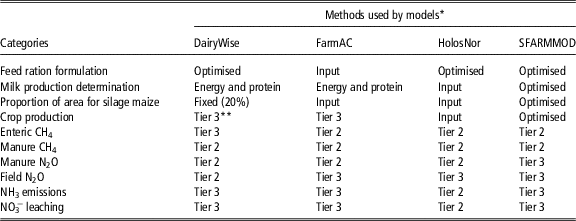
The models used were DairyWise, developed in The Netherlands (Schils et al., Reference Schils, de Haan, Hemmer, van den Pol-van Dasselaar, De Boer, Evers, Holshof, van Middelkoop and Zom2007), FarmAC, developed as part of an EU project (Hutchings and Kristensen, 2015), HolosNor, developed in Norway (Bonesmo et al., Reference Bonesmo, Skjelvag, Janzen, Klakegg and Tveito2012), and SFARMMOD, developed in the UK (Annetts and Audsley, Reference Annetts and Audsley2002). DairyWise and HolosNor are specifically dedicated to dairy farming whereas FarmAC and SFARMOD can simulate a wider range of farm types. The choice of models used depended on who could obtain funding via the Modelling European Agriculture with Climate Change for Food Security (MACSUR) project (www.macsur.eu). An overview of the models is given in Table 1, with additional details in the Supplementary Material S1. Some models could simulate off-farm GHG emissions, such as pre- or post-farm emissions, and/or emissions associated with the use of farm machinery. However, these emission sources are not part of the agricultural emissions in the ESR, so were omitted from the comparison. Changes in the carbon (C) sequestered in the soil are part of the ESR but as this could not be simulated by all models, it was also omitted from the comparison. Steady-state simulations with no change in the C sequestered were used for those models that included this aspect. Global warming potentials of methane (CH4) and N2O are 28 and 265 times higher than that of CO2, respectively, for a given 100 year time horizon (Myhre et al., Reference Myhre, Shindell, Bréon, Collins, Fuglestvedt, Huang, Koch, Lamarque, Mendoza, Nakajima, Robock, Stephens and Zhang2013).
Overview of the methods used by the models to calculate key farm characteristics and emissions

N2O=nitrous oxide; CH4=methane.
* See Supplementary Material S1.
** Tier 2=Tier 2, IPCC (2006); Tier 3=modified Tier 2 and/or dynamic modelling.
Scenarios
Each model simulated eight scenarios within a factorial design consisting of two climates, two soil types and two feeding systems. The two climates were cool with moderate rainfall (Eindhoven, The Netherlands; ‘Cool’) and warm with high rainfall (Santander, Spain; ‘Warm’). The Cool climate had a mean annual temperature of 9.6°C and a mean annual precipitation of 757 mm. The Warm climate had a mean annual temperature 14.3°C and a mean annual precipitation of 1268 mm. The characteristics of the Sandy soil were 60% sand, 10% silt, 30% clay and the Clayey soil were 10% sand, 45% silt, 45% clay. For both soil types, the pH >6, <7.5 and soil depth was 1 m. For HolosNor, the maximum permissible clay content allowed by the model (35%) was used (Skjelvåg AO, Ås, 2016, personal communication).
The choice of scenarios was intended to provoke noticeable responses from the models whilst remaining within the range of conditions for European dairy production. The choice of climates was also determined by the need to access advice concerning climate-related farm management information. Grass has an energy:protein ratio that is sub-optimal for effective utilisation of the protein for milk production, so must be supplemented with an energy-rich feed when formulating diets. This is commonly provided using either an imported cereal or on-farm maize silage, so two cropping systems were simulated, one consisting of grass only and other of grass and maize silage.
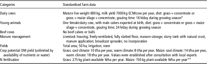
The participants agreed a set of farm structure and management characteristics and parameters (Table 2). The GHG emissions intensity of milk production decreases with increasing annual milk production per cow (Casey and Holden, Reference Casey and Holden2005; Gerber et al., Reference Gerber, Vellinga, Opio and Steinfeld2011), so it was necessary to standardise this factor. To avoid excessive externalising of GHG emissions through high imports of energy concentrates, we chose to simulate a production system with a moderate production of 7000 kg ECM/cow per year.
Standardised farm data

DM=dry matter; N=nitrogen.
* Cool climate; May to September, warm climate; March to November.
** Fertiliser type urea, with all fertiliser N considered plant-available. For animal manure, plant-available N was equal to the mineral N present. The total N application in manure was not permitted to exceed 250 kg N/ha per year for permanent grassland and 170 kg N/ha per year for maize silage. Manure was only exported if these application rates would otherwise be exceeded.
Complete standardisation of scenarios was not possible as all models required additional model-specific inputs or parameters. To internalise model responses, the exchange of material with off-farm systems was minimised. This meant that within realistic constraints (e.g. maintaining a realistic balance between energy and protein in cattle diets), the amount of imported animal feed and manure and the export of silage and manure was minimised. As the milk yield per cow, the weight of the mature dairy cows and the number of young stock per mature dairy cow were standardised, the number of livestock that could be carried on the farm was determined by each model’s prediction of: (i) the diet necessary to achieve the specified milk yield and growth of immature livestock; and (ii) the capacity of the farm to produce roughage feed. HolosNor required the number of animals as an input; therefore, the number of animals in each scenario was inputted to HolosNor from FarmAC.
The statistical significance of the differences between models for the selected management variables and the estimated GHG emissions was determined using the Friedman test, (Friedman, 1940) followed by the post hoc Nemenyi test (Nemenyi, Reference Nemenyi1963). The analysis was undertaken using the Friedman.test and posthoc.friedman.nemenyi.test function from the PMCMR package (Pohlert, Reference Pohlert2014) of R programming language. The corresponding analysis for differences between scenarios was determined using the anova function of the R programming language. Differences were considered significant if P<0.05 or less.
Results
Production characteristics
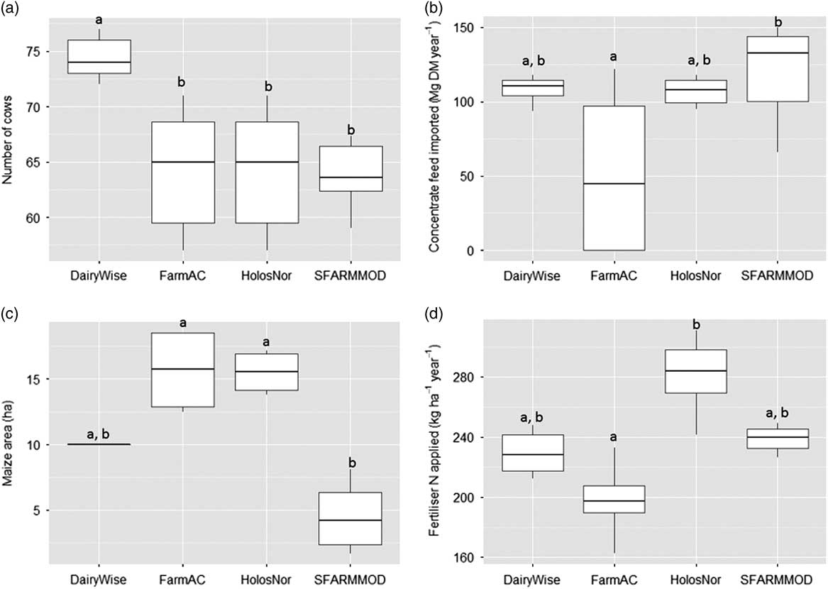
DairyWise predicted a significantly higher number of dairy cows could be maintained than the other models (Figure 1a). This was not due to lower values for the dry matter (DM) intake necessary to achieve the prescribed production; cow DM intake was 16.5, 15.6, 17.6 and 16.0 kg/day for DairyWise, FarmAC, HolosNor and SFARMOD, respectively, and for the followers, 6.0, 5.7, 7.1 and 4.8 kg/day, respectively. The median milk production values ranged from 10 360 l/ha for DairyWise to 8835 l/ha for HolsNor. The variation between scenarios was greatest for FarmAC (HolosNor used the same livestock numbers as FarmAC). There were significant differences between models in the amounts of concentrate feed imported (Figure 1b), reflecting the differences in the diet predicted or considered necessary to achieve the target milk production specified. The area dedicated to maize silage production on grass/maize farms was significantly lower for SFARMMOD than for the other models (Figure 1c). Note that for DairyWise, the area would have been higher, had the model not included a cap of 20% of field area that could be allocated to maize cultivation. There were significant differences between models in the amounts of fertiliser N applied (Figure 1d).
Predicted number of dairy cows (a), amount of concentrate feed imported (Mg dry matter (DM)/year) (b), area of maize on farms growing both grass and maize (ha) (c) and fertiliser N applied (kg/ha per year) (d). The boxplots show the data median and quartiles of the eight dairy farming scenarios. a,bDifferences between model results are not significantly different from one another if they share the same letter.

Farm-scale greenhouse gas emissions
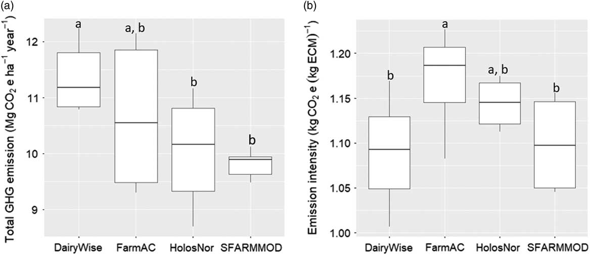
Total GHG emissions expressed on an area basis (‘area emission intensity’; kg CO2e/ha per year) were highest in DairyWise (Figure 2a), significantly higher in relation to HolosNor and SFARMMOD, with the range between models equivalent to 18% of the mean of models. This mainly reflects the significantly higher number of livestock predicted by DairyWise, as can be seen by expressing emissions on the basis of a unit mass of milk (‘milk emission intensity’; kg CO2e/(kg ECM)); the range between models is reduced to 6% of the mean of models, although there were still significant differences between models (Figure 2b). To prevent variations in livestock number from masking other differences between the models, the emissions from the on-farm sources will here be expressed as milk intensities rather than area intensities. Note that no allocation method was used when calculating the milk intensities (see Supplementary Material S1).
Total greenhouse gas (GHG) emissions from all sources, expressed as an area emission intensity (kg carbon dioxide equivalents (CO2e)/ha per year) (a) and as a milk emission intensity (kg CO2e/(kg ECM)) (b). The boxplots show the data median and quartiles. a,bDifferences between models are not significantly different from one another if they share the same letter.

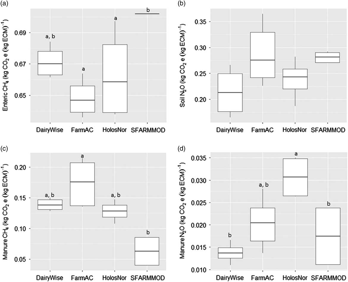
The enteric CH4 emissions simulated by SFARMMOD were significantly greater than those by FarmAC and HolosNor (Figure 3a). SFARMMOD estimates enteric CH4 emissions from milk production, hence the lack of variation between scenarios. There were no significant differences between the estimates of field N2O emissions from the different models (Figure 3b). The manure CH4 emissions estimated by SFARMMOD were lower than those of the other models, significantly so compared with FarmAC (Figure 3c). Manure N2O emissions (Figure 3d) estimated by HolosNor were higher than those of the other models, significantly so compared with DairyWise and SFARMMOD.
Direct greenhouse gas (GHG) emissions; enteric methane (CH4) emissions (a), soil nitrous oxide (N2O) emissions (b), manure CH4 (c) and manure N2O emissions (d) (kg carbon dioxide equivalents (CO2e)/(kg ECM)). The boxplots show the data median and quartiles. a,bDifferences between models are not significantly different from one another if they share the same letter.

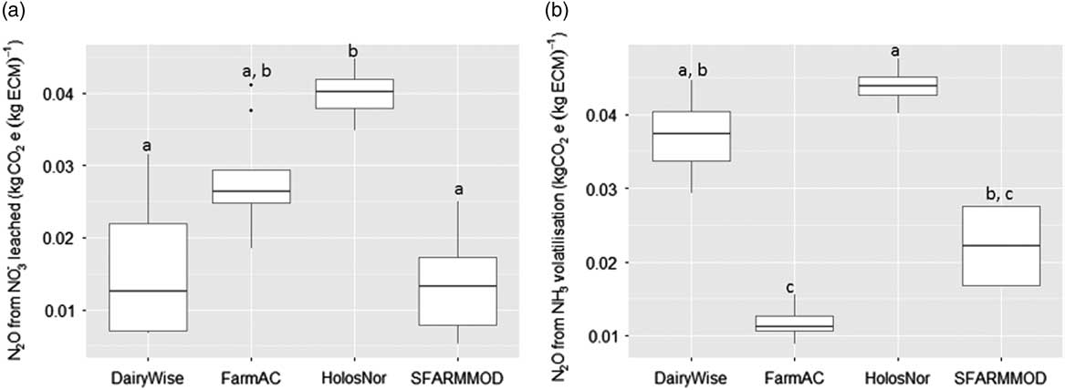
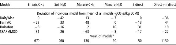
There were significant differences between models for the N2O emissions from both NH3 volatilisation and NO3 − leaching (Figure 4). The emissions estimated by HolosNor were higher than by the other models, significantly so in some instances. For FarmAC, the emissions resulting from NO3 − leaching were particularly variable between scenarios. The variation in GHG emissions from different sources between models is shown in Table 3. For each source, the mean of the emissions for the four models is subtracted from the emission for the individual model. The differences between models led to differences in the ranking of scenarios. DairyWise ranked the Cool climate higher than the Warm climate and thereafter Grass only higher than Grass/maize. FarmAC, HolosNor and SFARMMOD ranked grass only higher than grass/maize but there were no clear rankings for climate and soil.
Indirect nitrous oxide (N2O) emissions resulting from leaching of nitrate (NO3 −) (a) and from volatilisation of ammonia (NH3) from manure management and field-applied manure (b) (kg carbon dioxide equivalents (CO2e)/(kg ECM)). The boxplots show the data median and quartiles. a,b,cDifferences between models are not significantly different from one another if they share the same letter.

Variation between models in the direct and indirect greenhouse gas (GHG) emissions, relative to the mean of all models

CH4=methane; N2O=nitrous oxide.
* No allocation method used to partition emissions between milk and meat production (see Supplementary Material S1)
Differences between scenarios
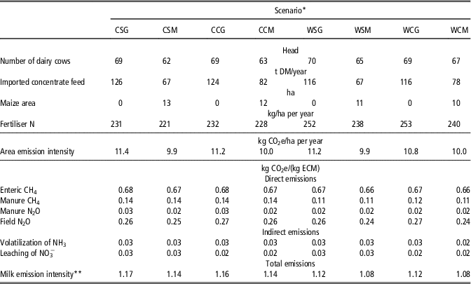
The production characteristics, and area and milk intensities for the different scenarios, averaged across models, are shown in Table 4. There were statistically significant differences between the feeding systems, with the Grass only system requiring more concentrate feed (1.75 v. 1.13 Mg DM/cow per year), carrying a higher number of cows (69.3 v. 64.2 head) and receiving more N fertiliser (242 v. 232 kg N/ha per year). Significantly more N fertiliser was applied under the Warm climate than under the Cool (246 v. 228 kg/ha per year). The area emission intensity was around 11% greater for the Grass only system than for the Grass/maize (11.1 kg v. 10.0 kg CO2e/ha per year). When expressed as milk emission intensities (kg CO2e/(kg ECM)), the emissions under the Cool climate were significantly greater than under the Warm climate for enteric CH4 (0.673 v. 0.669), manure CH4 (0.259 v. 0.251), manure N2O (0.025 v. 0.017) and the indirect N2O emission resulting from NH3 volatilisation (0.030 v. 0.028). The emissions for the Grass only were significantly greater than for the Grass/maize for enteric CH4 (0.677 v. 0.666), soil N2O (0.264 v. 0.247), manure CH4 (0.128 v. 0.124), manure N2O (0.022 v. 0.020), and the indirect N2O emission resulting from NH3 volatilisation (0.030 v. 0.028). The indirect N2O emission from NO3 − leaching was significantly higher for Sandy soil than Clayey soil (0.028 v. 0.020). At the farm scale, the milk intensities were significantly higher for Grass only than for Grass/maize (1.119 v. 1.084) and for the Cool climate than for the Warm (1.127 v. 1.076). Across scenarios, enteric CH4 and field N2O emissions were the major contributors to total GHG emissions.
Summary of results for the different scenarios

DM=dry matter; N=nitrogen; CH4=methane; N2O=nitrous oxide; NO3 −=nitrate.
* Cxx=Cool climate, Wxx=Warm climate, xSx=Sandy soil, xCx=Clayey soil, xxG=Grass only, xxM=Grass and maize.
** No allocation method used to partition emissions between milk and meat production (see Supplementary Material S1).
Discussion
Differences in production characteristics
The scenario specifications defined key production characteristics and yet achieving complete standardisation of farm management was not possible. The models differed both in their description of biophysical responses/feedback mechanisms and in the extent to which management functions were internalised. For example, when estimating the livestock number that could be carried on the farm, the DairyWise predictions were 15% higher than the other models (Figure 1a). This was due partly to a higher efficiency of the use of feed for milk production; the major drivers of production (DM intake, import of concentrate feed and available N used for crop production) being similar or the same as the other models. To achieve an appropriate feed ration on the Grass only farms, all models predicted it was necessary to import cereal feed. This import of feed increases the number of livestock that can be carried on the farm. As maize silage has a higher energy:protein ratio than grass, an appropriate feed ration could be more easily achieved from within the farms’ resources when maize silage was available on the farm. Consequently, three of the four models found the need to import cereal-based feed was lower for the Grass/maize system than for the Grass only system and hence fewer livestock were carried (Figure 1b); the exception being DairyWise. In DairyWise, the maximum percentage of the area of maize silage (20%) permitted is embedded in the model, corresponding to the derogation obtained by the Netherlands under the EU Nitrates Directive (European Commission, 1991 and 2014), so a higher import of concentrates is necessary to achieve an appropriate feed ration. Even the remaining models show substantial differences in the area allocated to maize silage production (Figure 1c), reflecting the differences in the definition of an appropriate feed ration and the maize silage production predicted per unit area. This highlights a major difference between farm-scale models and those of individual farm components such as crops; the latter are commonly driven by external management variables whereas these are internalised to a varying extent within the farm-scale models.
Finally, the application of N fertiliser varied between models (Figure 1d). As the total amount of plant-available N applied was prescribed here and were different for grass and maize, the differences in the application of N fertilizer reflect the differences between models in the estimation of the plant-availability of N in the animal manure, and for Grass/maize system, the relative areas allocated to grass and maize cultivation. This in turn reflects differences in the N losses occurring in the manure management system. The farm characterisation specified a higher input of plant-available N to grassland than to maize, so differences between models in the areas used to produce maize silage also lead to differences in the farm-scale demand for fertiliser N.
Differences in greenhouse gas emissions
The scenario-averaged area emission intensity was highest for DairyWise (Figure 2a). This was mainly due to the higher number of livestock that this model predicted could be supported on the farms, as the differences between models decrease when emissions are expressed as milk intensities (Figure 2b). The variation in enteric CH4 emissions (Figure 3a) has complex origins. The models differed in the methods used to determine the quantity and quality of feed appropriate to achieve the specified milk production per cow. As feed quality is predicted by DairyWise, it could not be standardised here, meaning there were differences between models in the feed quality. Finally, there were differences in methods used to model enteric CH4 emissions, which varied from a national Tier 3 method with varying emission factors per feedstuff (DairyWise), through the IPCC methodology (FarmAC, HolosNor), to a fixed factor based on milk production (SFARMMOD).
The differences between estimates of N2O emissions from the soil were not significant (Figure 3b), but this was due to the substantial variation between models in their response to the scenarios. All models use algorithms similar to those used by IPCC (2006) and so are driven by the total amount of N entering the soil. The total input of plant-available N (manure plus fertiliser) was prescribed here so the crop production was largely decoupled from the behaviour of the livestock and manure management modules. However, the estimates of the total N input to the soil differed between models, as differences in the estimated loss of N in the manure management system meant that they differed in their assessment of the plant-availability of N in the manure ex storage (the lower the plant-availability in the manure, the higher the total manure N input). Furthermore, the total plant-available N application to grass was prescribed to be higher than that to maize, so differences between models in the allocation of land to these two crops affected the farm scale input of N to the soil for the grass/maize systems.
The differences in GHG emissions from manure (Figure 3c and d) reflect differences in the methodologies used (particularly emission factors) and in the throughput of manure DM and N, resulting from differences in the methods used to estimate DM and N excretion. The significant differences in indirect GHG emissions associated with NH3 volatilisation (Figure 4a) reflect differences in assumptions made or the methodology used. In particular, in the DairyWise simulations, a high DM content of the applied slurry was assumed, leading to high field NH3 emissions. In the FarmAC simulations, a lower manure DM content was assumed and in SFARMMOD, a constant factor independent of manure DM.
The low indirect emissions of N2O associated with NO3 − leaching predicted by DairyWise (Figure 4b) is because it simulated a large N loss through denitrification on the clayey soil. The small effect of soil type on the HolosNor simulations were because this model uses a leaching fraction that is not sensitive to soil type. In contrast, FarmAC was highly sensitive to soil type, especially in the Warm climate due to the higher drainage.
The total GHG emissions calculated by the different models were similar but this disguised differences between estimates of all the contributory emissions (Table 3). Nevertheless, all models indicated that enteric CH4 was the major source, followed by soil N2O emissions, and that the two together contributed more than half the total emissions. This would be expected from earlier investigations (Food and Agriculture Organisation, 2010; Gerber et al., Reference Gerber, Vellinga, Opio and Steinfeld2011; Alemu et al., Reference Alemu, Janzen, Little, Hao, Thompson, Baron, Iwaasa, Beauchemin and Kröbel2017). Furthermore, all models ranked the importance of the remaining sources in the same order; manure CH4>indirect emissions>manure N2O. This is important, as the ranking of targets for mitigation measures is a common reason for constructing such models (Cullen and Eckard, Reference Cullen and Eckard2011; Del Prado et al., Reference Del Prado, Crosson, Olesen and Rotz2013). In contrast, the differences between the ranking of scenarios between models shows that there can be systematic variations in the responses to climate and farm management.
Variation between scenarios might be expected to increase with model complexity, as this should increase the capacity to reflect the effect of different management strategies (Beukes et al., Reference Beukes, Gregorini and Romera2011). Cullen and Eckard (Reference Cullen and Eckard2011) estimated GHG emissions for four locations in Australia and found the emissions estimated using the complex, dynamic model DairyMod (Johnson et al., Reference Johnson, Chapman, Snow, Eckard, Parsons, Lambert and Cullen2008) to be between +10% and −30% of the values estimated by an inventory method, depending on location. The majority of the variation between the two methods arose from differences between locations in the direct and indirect N2O emissions predicted by the complex model. In the current study, the range of milk emission intensities, relative to the model returning the lowest estimate, was 4% to 9% for the Cool climate and 13% to 16% for the Warm climate.
In O’Brien et al. (Reference O’Brien, Shalloo, Buckley, Horan, Grainger and Wallace2011), the use of locally determined rather than default parameters for the IPCC (2006) methodology led to a reduction in estimated GHG emissions of about 13%. In this study, the emission factors in FarmAC and HolosNor were adjusted to the IPCC (2006) default values for the relevant climate whereas the parameter values are not climate-sensitive in DairyWise and SFARMOD. As the latter two models were developed in The Netherlands and UK, respectively, this may explain the larger variation between the model emission estimates for the Warm climate.
Effect of scenarios
More concentrate feed was required to provide a balanced diet in the Grass only system than the Grass/maize system (Table 4). This meant that the total amount of feed available on the grass only farms was greater than for the Grass/maize system, so more cows could be carried and the area emission intensity was higher. Less fertiliser is applied to the grass/maize system than the Grass only system, as the application of plant-available N specified for maize was lower than that for grass. Expressed in terms of milk emission intensities, manure CH4 and N2O emissions (direct and from NH3 volatilisation) were lower under the Warm climate, due to the shorter housing period and therefore lower annual manure production. We have no immediate explanation for the higher enteric CH4 emission under the Cool climate but note that is a small effect (1% difference). The higher emissions from enteric fermentation, manure and soil under the Grass v. the Grass/maize system may reflect a lower ability to construct a balanced feed ration with grass as the only roughage feed and therefore a lower efficiency of utilisation of feed for milk production in the former. This would increase the flow of DM and N through the livestock and manure management, per unit mass of milk produced. The N2O emissions associated with NO3 − leaching were greater for the Sandy than Clayey soil, due to the higher drainage. The lower farm-scale milk emission intensity in the Warm climate compared with the Cool mainly reflected the lower emissions associated with manure management (79% of difference) whereas the difference between the Grass and Grass/maize systems was mainly associated with the soil N2O emission (47%).
The total model-averaged area emission intensities calculated here are within the range 9.6–11.8 kg CO2e/ha per year found for Ireland by O’Brien et al. (Reference O’Brien, Shalloo, Buckley, Horan, Grainger and Wallace2011), similar to the 11.0 and 9.5 kg CO2e/ha per year found for a farm in the USA by Veltman et al. (Reference Veltman, Jones, Gaillard, Cela, Chase, Duval, Izaurralde, Ketterings, Li, Matlock, Reddy, Rotz, William, Vadas and Jolliet2017), lower than the 12.1 kg CO2e/ha per year found for New Zealand by Beukes et al. (Reference Beukes, Gregorini and Romera2011) but higher than that calculated using the relationship with milk production per unit area found by Christie et al. (Reference Christie, Rawnsley and Eckard2011) (adjusted to remove non-ESR emissions). However, as noted by Christie et al. (Reference Christie, Rawnsley and Eckard2011), comparing the results of different studies is difficult, due to variations in the methods used, so we here draw no other conclusion than that the results are within the range found in other studies and that the scenarios we chose were indeed an adequate basis for investigating the process of comparing the models.
Comparing greenhouse gas emissions from dairy cattle farm models
The advantage of using farm-scale models of dairy cattle production in the context of the ESR, particularly in relation to their ability to predict the consequences of mitigation measures on emissions and production, arises mainly because of their ability to account for the on-farm feedback processes. However, as we have shown here, the same feedback processes sometimes make it difficult to standardise all aspects of farm-scale scenarios and complicate the process of understanding the reasons for differences between model results. The maximum difference between models in area emission intensity was equivalent to about 18% of the mean of all models, equivalent to about half the average ESR reduction demand. The magnitude of this variation underscores the importance of understanding and assessing the credibility of farm models when they are used as part of national GHG emission accounting, and in gaining acceptance by producers, where a Member State choses to introduce GHG accounting at the farm scale. We believe this justifies further investment in methodologies and tools to support the comparison of farm-scale models. That investment needs to include the development of a wider range of scenarios, designed to encompass all European dairy production, and software tools to compare, analyse and present the large amount of data generated.
Conclusions
Based on the four farm-scale models used here, we conclude that there can be important differences between models in the GHG emissions predicted at the source and farm scales. These variations between models arise because of differences in the simulation of the processes and feedback loops driving production and emission, and the extent to which management functions are internalised. These model features complicate the standardisation of farm characteristics and management in scenarios and the interpretation of results. Nevertheless, we conclude that comparing the results of applying farm-scale models to a wide range of scenarios is a useful process for quality assurance and review, and that further investment in the development of scenarios and software tools is justified.
Acknowledgements
Authors acknowledge the financial support from the European Commission (AIR3-CT94-1584, ECFARM project), UK Government Department for Agriculture and Rural Affairs (WA0801, MEASURES project), Ministry of Agriculture Fisheries and Food/Biotechnology and Biological Sciences Research Council who funded parts of the development of SFARMMOD. Thanks also to Jordi Doltra for his insight into dairy farm management in Northern Spain, Arne Oddvar Skjelvåg for preparing the soil and climate data for HolosNor simulations, and Bente Aspeholen Åby, Sissel Hansen and Tonje Storlien for sharing their experiences with HolosNor. This paper was supported by the FACCE-JPI knowledge hub Modelling European Agriculture with Climate Change for Food Security (MACSUR). National funding was received from the Norwegian Research Council and BBSRC (BB/N00485X/1 and BB/K010301/1 projects).
Supplementary material
To view supplementary material for this article, please visit https://doi.org/10.1017/S175173111700338X