1. Introduction
The flashing Brownian ratchet of Ajdari and Prost (Reference Ajdari and Prost1992) is a time-inhomogeneous diffusion process that alternates between two regimes, a one-dimensional Brownian motion and a Brownian ratchet, the latter being a one-dimensional diffusion process that drifts towards a minimum of a periodic asymmetric sawtooth potential. It models the motion of a particle in a diffusive medium subject to a potential that is ‘flashed’ on and off, on and off, periodically. The result is directed motion (see, e.g., Ethier and Lee (Reference Ethier and Lee2018)).
To better understand this phenomenon, J. M. R. Parrondo proposed in 1996 a toy model of the flashing Brownian ratchet involving two coin-tossing games, game A, corresponding to Brownian motion, and game B, corresponding to the Brownian ratchet. Each of the games, A and B, is individually fair or losing, while the periodic sequence of games
 $ABB\,ABB\,ABB\,\ldots$
, corresponding to the flashing Brownian ratchet, is winning. As explained by Marzuoli (Reference Marzuoli2009) in a different context,
Toy models in theoretical physics are invented to make simpler the modelling of complex physical systems while preserving at least a few key features of the originals. Sometimes toy models get a life of their own and have the chance of emerging as paradigms.
That is exactly what has happened with Parrondo’s games. They have emerged as a paradigm for a much broader phenomenon. The Parrondo effect (or Parrondo’s paradox) can be said to occur if there is a reversal in direction in some system parameter when two similar dynamics are combined. There are a variety of examples in the physical and biological sciences where the Parrondo effect, in the wide sense, has been observed. Some of these examples are discussed in the review papers of Harmer and Abbott (Reference Harmer and Abbott2002), Abbott (Reference Abbott2010), and Cheong et al. (Reference Cheong, Koh and Jones2019).
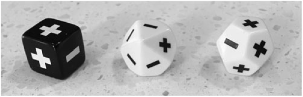
Parrondo dice. The games defined above (1) in terms of biased coins can be played with dice. Game A uses the black die (3
 $+$
, 3 –), while game B uses the white dice, namely (1
 $+$
, 9 –) when capital is congruent to 0 (mod 3) and (9
 $+$
, 3 –) otherwise. The player wins one unit with a plus sign and loses one unit with a minus sign.

The literature on the Parrondo effect now comprises hundreds of papers, but its intersection with the probability literature is relatively small. Included in that intersection are a number of studies of the asymptotic behavior of Parrondo’s games, namely Harmer et al. (Reference Harmer, Abbott and Taylor2000a), Percus and Percus (Reference Percus and Percus2002), Pyke (Reference Pyke, Moore, Froda and Léger2003), Behrends (Reference Behrends, Gingl, Sancho, Schimansky-Geier and Kertesz2004), Costa et al. (Reference Costa, Fackrell, Taylor, Nowak and Szajowski2005), Key et al. (Reference Key, Kłosek and Abbott2006), Ethier and Lee (Reference Ethier and Lee2009), and Rémillard and Vaillancourt (Reference Rémillard and Vaillancourt2019). Also included are several applied probability papers in areas such as information theory (Harmer et al. (Reference Harmer, Broomhead, Luchinskaya, McClintock and Mullin2000b)), reliability theory (Di Crescenzo (Reference Di Crescenzo2007)), gambling (Ethier and Lee (Reference Ethier and Lee2010)), quantum random walks (Machida and Grünbaum (Reference Machida and Grünbaum2018)), and renewal reward theory (Miles et al. (Reference Miles, Lawley and Keener2018)).
Our focus in this paper will be on Parrondo’s capital-dependent coin-tossing games, A and B (Harmer and Abbott (Reference Harmer and Abbott1999)). For simplicity we omit the bias parameter, so that both games are fair. The Parrondo effect appears when games A and B, played in a random or periodic sequence, form a winning game. Let us define a p-coin to be a coin with probability p of heads. In Parrondo’s original games, game A uses a fair coin, while game B uses two biased coins, a
 $p_0$
-coin if the capital is congruent to 0 (mod 3) and a
 $p_1$
-coin otherwise, where
 \begin{equation}p_0=\frac{1}{10}\quad\text{and}\quad p_1=\frac34.\end{equation}
The player wins one unit with heads and loses one unit with tails. (These coins can be physically realized with dice; see Figure 1 for an alternative, but equivalent, description of the games.) Both games are fair, but the random mixture, denoted by
 $\frac12 A+\frac12 B$
and interpreted as the game in which the toss of a fair coin determines whether game A or game B is played, has the long-term cumulative profit per game played (hereafter, rate of profit)
 \begin{equation*}
\mu\big({\textstyle\frac12}A+{\textstyle\frac12}B\big)=\frac{18}{709}\approx0.025\,3879,\end{equation*}
and the pattern ABB, repeated ad infinitum, has rate of profit
 \begin{equation}\mu(ABB)=\frac{2416}{35\,601}\approx0.067\,8633.\end{equation}
Dinis (Reference Dinis2008) found that the pattern ABABB has the highest rate of profit, namely
 \begin{equation}\mu(ABABB)=\frac{3\,613\,392}{47\,747\,645}\approx0.075\,6769.\end{equation}
These rates of profit are rather modest. Can we modify the games to make the rates of profit more substantial? To put it more precisely, how large can the rate of profit be if we vary the parameters of the games, subject to a fairness constraint? We will focus on periodic sequences, where the rates of profit tend to be larger than with random sequences.
Game A is always the same fair-coin-tossing game. With
 $r\ge3$
an integer, game B is a mod r capital-dependent game that uses two biased coins, a
 $p_0$
-coin (
 $p_0<1/2$
) if capital is congruent to 0 (mod r), and a
 $p_1$
-coin (
 $p_1>1/2$
) otherwise. The probabilities
 $p_0$
and
 $p_1$
must be such that game B is fair, which requires the constraint
 \begin{equation*}
(1-p_0)(1-p_1)^{r-1}=p_0\, p_1^{r-1},\end{equation*}
or equivalently,
 \begin{equation}p_0=\frac{\rho^{r-1}}{1+\rho^{r-1}}\quad\text{and}\quad p_1=\frac{1}{1+\rho}\end{equation}
for some
 $\rho\in(0,1)$
. The special case of
 $r=3$
and
 $\rho=1/3$
gives (1). The games are played in some pattern
 $\Gamma(A,B)$
, repeated ad infinitum. We denote the rate of profit by
 $\mu(r,\rho,\Gamma(A,B))$
, so that the rates of profit in (2) and (3) in this notation become
 $\mu(3,1/3,ABB)$
and
 $\mu(3,1/3,ABABB)$
.
How large can
 $\mu(r,\rho,\Gamma(A,B))$
be? The answer, perhaps surprisingly, is that it can be arbitrarily close to 1 (i.e. 100%).
 \begin{equation}\sup_{r\ge3,\,\rho\in(0,1),\,\Gamma(A,B)\,{arbitrary}}\mu(r,\rho,\Gamma(A,B))=1.\end{equation}
The proof is deferred to Section 4. Incidentally, the supremum in (5) is not achieved.
We can compute
 $\mu(r,\rho,\Gamma(A,B))$
for
 $r\ge3$
(the modulo number in game B) and pattern
 $\Gamma(A,B)$
as a function of
 $\rho$
(the parameter in (4)). Indeed, the method of Ethier and Lee (Reference Ethier and Lee2009) applies if r is odd, and generalizations of it apply if r is even; see Section 2 for details. For example,
 \begin{equation}\mu(3,\rho,ABB)=\frac{(1 - \rho)^3 (1 + \rho) (1 + 2 \rho + \rho^2 + 2 \rho^3 + \rho^4)}{3 + 12 \rho + 20 \rho^2 + 28 \rho^3 + 36 \rho^4 + 28 \rho^5 + 20 \rho^6 + 12 \rho^7 + 3 \rho^8}.\end{equation}
This and other examples suggest that typically
 $\mu(r,\rho,\Gamma(A,B))$
is decreasing in
 $\rho$
, hence maximized at
 $\rho=0$
. (There are exceptions, which include, when
 $r\ge3$
is odd,
 $AB^s$
with
 $s\ge3$
odd.) We excluded the case
 $\rho=0$
in (4), but now we want to include it. We find that
 \begin{equation}\mu(3,0,ABB)=\frac13\end{equation}
(by (6)) and
 \begin{equation}\mu(3,0,ABABB)=\frac{9}{25}.\end{equation}
This is already a substantial improvement over (2) and (3). Thus, we take
 $\rho=0$
in what follows.
For a given
 $r\ge3$
, we expect that we can maximize the rate of profit
 $\mu(r,0,\Gamma(A,B))$
with a pattern of the form
 \begin{equation}\Gamma(A,B)=(AB)^s B^{r-2}\end{equation}
for some positive integer s. Notice that this is ABB if
 $(r,s)=(3,1)$
and ABABB if
 $(r,s)=(3,2)$
.
Let us explain the intuition behind (9). Only the s plays of game A are random. Game B is deterministic and very simple: If capital is congruent to 0 (mod r), we lose one unit, otherwise we win one unit. Notice that cumulative profit remains bounded by r when game B is played repeatedly, hence cumulative profit per game played tends to 0 as the number of games played tends to infinity, and game B is (asymptotically) fair.
Clearly, the optimal strategy, if it were legal, would be to play game A when capital is congruent to 0 (mod r) and to play game B otherwise. With initial capital congruent to 0 (mod r), this strategy could be described as playing the pattern
 $(AB)^S B^{r-2}$
, where S is the geometric random variable equal to the number of plays of game A needed to achieve a win at that game. Of course, random patterns are not ordinarily considered, so (9) seems a reasonable nonrandom approximation for some positive integer s.
First, assume that r is odd and the initial capital is congruent to 0 (mod r). If all s plays of game A result in losses, the cumulative profit is
 $-1$
after one play of (9); otherwise it is r. If initial capital is congruent to
 $r-1$
(mod r), then after one play of (9), the cumulative profit is 1 with probability 1.
Second, assume that r is even, and again the initial capital is congruent to 0 (mod r). If the number of wins in the s plays of game A is 0, the cumulative profit is 0 after one play of (9); if the number of wins is between 1 and
 $r/2$
, inclusive, the cumulative profit is r; if the number of wins is between
 $r/2+1$
and r, inclusive, the cumulative profit is 2r; if the number of wins is between
 $r+1$
and
 $3r/2$
, inclusive, the cumulative profit is 3r; and so on. If the initial capital is congruent to
 $r-1$
(mod r), then after one play of (9), the cumulative profit is 0 with probability 1.
The probabilistic structure of capital growth after multiple plays of (9) can be analyzed precisely from these observations, and we can evaluate the exact rate of profit with the help of one additional step. The additional step, addressed in Section 3, is to evaluate the mean of a distribution that is similar to, but stochastically less than, the binomial distribution with parameters n and p. Although we need this mean only for
 $p=1-2^{-s}$
, where s is a positive integer, we treat the case of general p, anticipating that this distribution may have other applications.
Theorem 2. Let
 $r\ge3$
be an odd integer and s be a positive integer. Then
 \begin{equation}\mu(r,0,(AB)^sB^{r-2})=\frac{r}{2s+r-2}\;\frac{2^s-1}{2^s+1},\end{equation}
regardless of the initial capital.
Let
 $r\ge4$
be an even integer and s be a positive integer. Then
 \begin{equation}\mu(r,0,(AB)^sB^{r-2})=\begin{cases}\cfrac{r}{2s+r-2}\;\displaystyle{\sum_{k=0}^s\bigg\lceil\frac{2k}{r}\bigg\rceil\binom{s}{k}\frac{1}{2^s}}&\textit{if initial capital is even},\\ \noalign{\medskip}0&\textit{if initial capital is odd}.\end{cases}\end{equation}
The formula in (10) is consistent with (7) and (8). The sum in (11) is equal to
 $(2^s-1)/2^s$
if
 $s\le r/2$
and bounded below by
 $(2^s-1)/2^s$
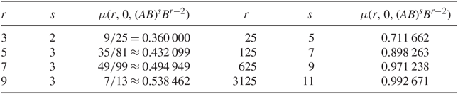
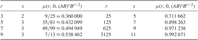
in general. Theorem 2 implies Theorem 1, as we will confirm later. The proof of Theorem 2 is deferred to Section 4. Table 1 illustrates (10) with several examples.
The rate of profit
 $\mu(r,0,(AB)^s B^{r-2})$
. Here, for a given odd r, we choose s to maximize
 $s'\mapsto\mu(r,0,(AB)^{s'} B^{r-2})$
. The results are rounded to six significant digits
We do not consider random mixtures
 $\gamma A+(1-\gamma)B$
of games A and B. Although we expect that the rate of profit, which we denote by
 $\mu(r,\rho,\gamma A+(1-\gamma)B)$
, can be made arbitrarily close to 1 by suitable choice of the modulo number r in game B, the parameter
 $\rho$
in (4), and the probability
 $\gamma$
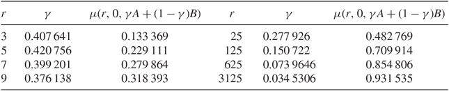
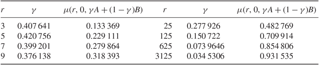
with which game A is played, we cannot prove it. However, see Table 2 for several examples.
The rate of profit
 $\mu(r,0,\gamma A+(1-\gamma)B)$
. Here, for a given odd r, we choose
 $\gamma$
to maximize
 $\gamma'\mapsto\mu(r,0,\gamma' A+(1-\gamma')B)$
. The results are rounded to six significant digits
2. Strong law of large numbers for periodic sequences of games
Ethier and Lee (Reference Ethier and Lee2009) proved a strong law of large numbers (SLLN) and a central limit theorem for periodic sequences of Parrondo games of the form
 $A^r B^s$
, repeated ad infinitum, where r and s are positive integers. Below we state a generalization of the SLLN to arbitrary patterns. Later we will weaken the hypotheses as needed.
First, it should be mentioned that several other authors have studied periodic sequences of Parrondo games. Pyke (Reference Pyke, Moore, Froda and Léger2003) discussed one example, AABB, which he regarded as the alternation of AA and BB. His method is sound but his stated ‘asymptotic average gain’ for that example is inaccurate (indeed,
 $\mu(3,1/3,AABB)=4/163\approx0.0245\,399$
), and the source of the error is unknown. Kay and Johnson (Reference Kay and Johnson2003) studied patterns of the form
 $A^r B^s$
in the context of history-dependent Parrondo games, and gave an expression for the rate of profit that is consistent with (12) below. Key et al. (Reference Key, Kłosek and Abbott2006), as well as Rémillard and Vaillancourt (Reference Rémillard and Vaillancourt2019), took a different approach, analyzing periodic sequences of Parrondo games in terms of transience to
 $\pm\infty$
and recurrence instead of in terms of the rate of profit.
Theorem 3. Let
 ${\textbf{\textit{P}}}_A$
and
 ${\textbf{\textit{P}}}_B$
be transition matrices for Markov chains in a finite state space
 $\Sigma$
. Let
 $C_1C_2\cdots C_t$
, where each
 $C_i$
is A or B, be a pattern of As and Bs of length t. Assume that
 ${\textbf{\textit{P}}}:={\textbf{\textit{P}}}_{C_1}{\textbf{\textit{P}}}_{C_2}\cdots{\textbf{\textit{P}}}_{C_t}$
is irreducible and aperiodic, and let the row vector
 $\boldsymbol{\pi}$
be the unique stationary distribution of
 ${\textbf{\textit{P}}}$
. Given a real-valued function w on
 $\Sigma\times\Sigma$
, define the payoff matrix
 ${\textbf{\textit{W}}}:=(w(i,j))_{i,j\in\Sigma}$
. Define
 $\dot{\textbf{\textit{P}}}_A:= {\textbf{\textit{P}}}_A\circ{\textbf{\textit{W}}}$
and
 $\dot{\textbf{\textit{P}}}_B:={\textbf{\textit{P}}}_B\circ{\textbf{\textit{W}}}$
, where
 $\circ$
denotes the Hadamard (entrywise) product, and put
 \begin{equation}\mu:= t^{-1}\boldsymbol{\pi}(\dot{\textbf{\textit{P}}}_{C_1}+{\textbf{\textit{P}}}_{C_1}\dot{\textbf{\textit{P}}}_{C_2}+\cdots+{\textbf{\textit{P}}}_{C_1}{\textbf{\textit{P}}}_{C_2}\cdots{\textbf{\textit{P}}}_{C_{t-1}}\dot{\textbf{\textit{P}}}_{C_t}){\boldsymbol{1}},\end{equation}
where
 ${\boldsymbol{1}}$
denotes a column vector of 1s with entries indexed by
 $\Sigma$
. Let
 $\{X_n\}_{n\ge0}$
be a nonhomogeneous Markov chain in
 $\Sigma$
with transition matrices
 ${\textbf{\textit{P}}}_{C_1}$
,
 ${\textbf{\textit{P}}}_{C_2}$
,
 $\ldots$
,
 ${\textbf{\textit{P}}}_{C_t}$
,
 ${\textbf{\textit{P}}}_{C_1}$
,
 ${\textbf{\textit{P}}}_{C_2}$
,
 $\ldots$
,
 ${\textbf{\textit{P}}}_{C_t}$
,
 ${\textbf{\textit{P}}}_{C_1}$
, and so on, and let the initial distribution be arbitrary. For each
 $n\ge1$
, define
 $\xi_n:= w(X_{n-1},X_n)$
and
 $S_n:= \xi_1+\cdots+\xi_n$
. Then
 $\lim_{n\to\infty}n^{-1}S_n=\mu$
almost surely (a.s.).
Remark 1. Fix positive integers r and s, put
 $t=r+s$
, and let
 $C_1=\cdots=C_r=A$
and
 $C_{r+1}=\cdots=C_{r+s}=B$
. Then this theorem is precisely the strong law of large numbers of Ethier and Lee (Reference Ethier and Lee2009). Actually, a few unnecessary hypotheses have been omitted in the formulation above, as explained below.
Proof of Theorem 3. The proof is identical to the proof of (Ethier and Lee
Reference Ethier and Lee2009, Theorem 6). However, here we have assumed fewer hypotheses and should explain why. First, it is unnecessary to assume that
 ${\textbf{\textit{P}}}_A$
and
 ${\textbf{\textit{P}}}_B$
are irreducible and aperiodic because that assumption is not needed. It is also unnecessary to assume that all cyclic permutations of
 ${\textbf{\textit{P}}}:= {\textbf{\textit{P}}}_{C_1}{\textbf{\textit{P}}}_{C_2}\cdots{\textbf{\textit{P}}}_{C_t}$
are irreducible and aperiodic because that assumption is redundant; it suffices that
 ${\textbf{\textit{P}}}$
itself be irreducible and aperiodic. Finally, we assumed in the original theorem that the Markov chain
 \begin{equation}(X_0,X_1,\ldots,X_t),(X_t,X_{t+1},\ldots,X_{2t}),(X_{2t},X_{2t+1},\ldots,X_{3t}),\ldots\end{equation}
is irreducible and aperiodic, and we claim that this assumption is also redundant. The state space
 $\Sigma^*$
of (13) is the set of
 $(x_0,x_1,\ldots,x_t)\in\Sigma^{t+1}$
such that
 \begin{equation*}\boldsymbol{\pi}(x_0){\textbf{\textit{P}}}_{C_1}(x_0,x_1){\textbf{\textit{P}}}_{C_2}(x_1,x_2)\cdots{\textbf{\textit{P}}}_{C_t}(x_{t-1},x_t)>0,\end{equation*}
and its transition matrix
 ${\textbf{\textit{Q}}}$
is given by
 \begin{align*}&{\textbf{\textit{Q}}}((x_0,x_1,\ldots,x_t),(x_t,x_{t+1},\ldots,x_{2t}))\\
&\qquad{}={\textbf{\textit{P}}}_{C_1}(x_t,x_{t+1}){\textbf{\textit{P}}}_{C_2}(x_{t+1},x_{t+2})\cdots{\textbf{\textit{P}}}_{C_t}(x_{2t-1},x_{2t}).\end{align*}
We use the fact that a necessary and sufficient condition for a finite Markov chain to be irreducible and aperiodic is that some power of its transition matrix has all entries positive. It is straightforward to show that
 ${\textbf{\textit{Q}}}^n$
has all entries positive if
 ${\textbf{\textit{P}}}^{n-1}$
does. Indeed,
 \begin{align}
&{\textbf{\textit{Q}}}^n((x_0,x_1,\ldots,x_t),(y_0,y_1,\ldots,y_t))\nonumber\\
&\qquad{}={\textbf{\textit{P}}}^{n-1}(x_t,y_0){\textbf{\textit{P}}}_{C_1}(y_0,y_1){\textbf{\textit{P}}}_{C_2}(y_1,y_2)\cdots{\textbf{\textit{P}}}_{C_t}(y_{t-1},y_t).
\end{align}
Because
 ${\textbf{\textit{P}}}$
is irreducible and aperiodic, so too is
 ${\textbf{\textit{Q}}}$
.
As an illustration, we can use (12) to confirm (2) and (3), in which case
 $\Sigma=\{0,1,2\}$
,
 \begin{equation*}
{\textbf{\textit{P}}}_A=\begin{pmatrix}0&\quad 1/2&\quad 1/2\\1/2&\quad 0&\quad 1/2\\1/2&\quad 1/2&\quad 0\end{pmatrix},\quad
{\textbf{\textit{P}}}_B=\begin{pmatrix}0&\quad 1/10&\quad 9/10\\1/4&\quad 0&\quad 3/4\\3/4&\quad 1/4&\quad 0\end{pmatrix},\end{equation*}
and the payoff matrix is
 \begin{equation*}{\textbf{\textit{W}}}=\begin{pmatrix}0&\quad 1&\quad -1\\-1&\quad 0&\quad 1\\ 1&\quad -1&\quad 0\end{pmatrix}.\end{equation*}
More generally, we wish to apply Theorem 3 with
 \begin{equation}
\Sigma=\{0,1,\ldots,r-1\}\end{equation}
(r is the modulo number in game B), the
 $r\times r$
transition matrices
 \begin{equation}
{\textbf{\textit{P}}}_A=\begin{pmatrix}0& \quad 1/2& \quad 0& \quad \cdots& \quad 0& \quad 0& \quad 1/2\\[2pt]
1/2& \quad 0& \quad 1/2& \quad \cdots& \quad 0& \quad 0& \quad 0\\[2pt]
0& \quad 1/2& \quad 0& \quad \cdots& \quad 0& \quad 0& \quad 0\\
\vdots& \quad \vdots& \quad \vdots& \quad & \quad \vdots& \quad \vdots& \quad \vdots\\[2pt]
0& \quad 0& \quad 0& \quad \cdots& \quad 0& \quad 1/2& \quad 0\\[2pt]
0& \quad 0& \quad 0& \quad \cdots& \quad 1/2& \quad 0& \quad 1/2\\[2pt]
1/2& \quad 0& \quad 0& \quad \cdots& \quad 0& \quad 1/2& \quad 0\end{pmatrix},\end{equation}
 \begin{equation}
{\textbf{\textit{P}}}_B=\begin{pmatrix}0& \quad p_0& \quad 0& \quad \cdots& \quad 0& \quad 0& \quad 1-p_0\\[2pt]
1-p_1& \quad 0& \quad p_1& \quad \cdots& \quad 0& \quad 0& \quad 0\\[2pt]
0& \quad 1-p_1& \quad 0& \quad \cdots& \quad 0& \quad 0& \quad 0\\
\vdots& \quad \vdots& \quad \vdots& \quad & \quad \vdots& \quad \vdots& \quad \vdots\\[2pt]
0& \quad 0& \quad 0& \quad \cdots& \quad 0& \quad p_1& \quad 0\\[2pt]
0& \quad 0& \quad 0& \quad \cdots& \quad 1-p_1& \quad 0& \quad p_1\\[2pt]
p_1& \quad 0& \quad 0& \quad \cdots& \quad 0& \quad 1-p_1& \quad 0\end{pmatrix},\end{equation}
where
 $p_0$
and
 $p_1$
are given by (4), and the
 $r\times r$
payoff matrix
 \begin{equation}
{\textbf{\textit{W}}}=\begin{pmatrix}0& \quad 1& \quad 0& \quad \cdots& \quad 0& \quad 0& \quad -1\\[1pt]
-1& \quad 0& \quad 1& \quad \cdots& \quad 0& \quad 0& \quad 0\\[1pt]
0& \quad -1& \quad 0& \quad \cdots& \quad 0& \quad 0& \quad 0\\
\vdots& \quad \vdots& \quad \vdots& \quad & \quad \vdots& \quad \vdots& \quad \vdots\\[1pt]
0& \quad 0& \quad 0& \quad \cdots& \quad 0& \quad 1& \quad 0\\[1pt]
0& \quad 0& \quad 0& \quad \cdots& \quad -1& \quad 0& \quad 1\\[1pt]
1& \quad 0& \quad 0& \quad \cdots& \quad 0& \quad -1& \quad 0\end{pmatrix}.
\end{equation}
There are five cases that we want to consider.
1. Let the pattern
 $C_1C_2\cdots C_t$
of Theorem 3 be arbitrary. If
$\rho>0$
and r is odd (
$\ge3$
), then
${\textbf{\textit{P}}}:= {\textbf{\textit{P}}}_{C_1}{\textbf{\textit{P}}}_{C_2}\cdots{\textbf{\textit{P}}}_{C_t}$
is irreducible and aperiodic.
2. Let the pattern
$C_1C_2\cdots C_t$
be arbitrary. If
$\rho>0$
, r is even (
$\ge4$
), and t is odd, then
${\textbf{\textit{P}}}$
is irreducible and periodic with period 2.3. Let the pattern
$C_1C_2\cdots C_t$
be arbitrary. If
$\rho>0$
, r is even (
$\ge4$
), and t is even, then
${\textbf{\textit{P}}}$
is reducible with two aperiodic recurrent classes, each of size
$r/2$
.4. Let the pattern
$C_1C_2\cdots C_t$
have the form
$(AB)^s B^{r-2}$
for a positive integer s. If
$\rho=0$
and r is odd (
$\ge3$
), then
${\textbf{\textit{P}}}:= ({\textbf{\textit{P}}}_A {\textbf{\textit{P}}}_B)^s({\textbf{\textit{P}}}_B)^{r-2}$
is reducible with one aperiodic recurrent class of size 2 and
$r-2$
transient states.5. Let the pattern
$C_1C_2\cdots C_t$
have the form
$(AB)^s B^{r-2}$
for a positive integer s. If
$\rho=0$
and r is even (
$\ge4$
), then
${\textbf{\textit{P}}}$
is reducible with two absorbing states and
$r-2$
transient states.








Theorem 3 applies directly only to Case 1. Nevertheless, the theorem can be extended so as to apply first to Cases 1 and 4 (Theorem 4), then to Cases 3 and 5 (Theorem 5), and finally to Case 2 (Theorem 6). We begin by generalizing Theorem 3 so as to apply to Cases 1 and 4.
Theorem 4. Theorem 3 holds with ‘is irreducible and aperiodic’ replaced by ‘has only one recurrent class, which is aperiodic’.
Proof.Assume that
 ${\textbf{\textit{P}}}$
has only one recurrent class, which is aperiodic. Let
 $\Sigma_0\subset\Sigma$
be the unique recurrent class. The stationary distribution
 $\boldsymbol{\pi}$
of
 ${\textbf{\textit{P}}}$
is unique and satisfies
 $\boldsymbol{\pi}(x)>0$
if
 $x\in\Sigma_0$
and
 $\boldsymbol{\pi}(x)=0$
otherwise. For some
 $n\ge2$
,
 ${\textbf{\textit{P}}}^{n-1}(x_t,y_0)>0$
for all
 $x_t,y_0\in\Sigma_0$
. With the help of (14) we find that
 ${\textbf{\textit{Q}}}^n$
has all entries positive, hence
 ${\textbf{\textit{Q}}}$
is irreducible and aperiodic.
An example may help to clarify this argument. Consider the special case of (15)–(18) (with (4)) in which
 $\rho=0$
and
 $r=3$
, and let
 $t=3$
,
 $C_1=A$
, and
 $C_2=C_3=B$
. Then
 $\boldsymbol{\pi}=(2/3,0,1/3)$
, and the state space for the Markov chain
 $(X_0,X_1,X_2,X_3)$
,
 $(X_3,X_4,X_5,X_6)$
,
 $\ldots$
is
 $\Sigma^*=\{(0,1,2,0), (0,2,0,2), (2,0,2,0), (2,1,2,0)\}$
with corresponding transition matrix
 \begin{equation*}
{\textbf{\textit{Q}}}=\begin{pmatrix}1/2& \quad 1/2& \quad 0& \quad 0\\[2pt] 0& \quad 0& \quad 1/2& \quad 1/2\\[2pt] 1/2& \quad 1/2& \quad 0& \quad 0\\[2pt] 1/2& \quad 1/2& \quad 0& \quad 0\end{pmatrix},\end{equation*}
which is irreducible and aperiodic.
The remainder of the proof follows that of (Ethier and Lee Reference Ethier and Lee2009, Theorem 6).
We turn to Cases 3 and 5, which require a new formulation of Theorem 3, the difficulty being that the limit in the SLLN depends on the initial distribution of the underlying Markov chain.
Theorem 5. Let
 ${\textbf{\textit{P}}}_A$
and
 ${\textbf{\textit{P}}}_B$
be transition matrices for Markov chains in a finite state space
 $\Sigma$
. Let
 $C_1C_2\cdots C_t$
, where each
 $C_i$
is A or B, be a pattern of As and Bs of length t. Assume that
 ${\textbf{\textit{P}}}:= {\textbf{\textit{P}}}_{C_1}{\textbf{\textit{P}}}_{C_2}\cdots{\textbf{\textit{P}}}_{C_t}$
is reducible with two recurrent classes
 $R_1$
and
 $R_2$
, both of which are aperiodic, and possibly some transient states, and let the row vectors
 $\boldsymbol{\pi}_1$
and
 $\boldsymbol{\pi}_2$
be the unique stationary distributions of
 ${\textbf{\textit{P}}}$
concentrated on
 $R_1$
and
 $R_2$
, respectively. Given a real-valued function w on
 $\Sigma\times\Sigma$
, define the payoff matrix
 ${\textbf{\textit{W}}}:= (w(i,j))_{i,j\in\Sigma}$
. Define
 $\dot{\textbf{\textit{P}}}_A:= {\textbf{\textit{P}}}_A\circ{\textbf{\textit{W}}}$
and
 $\dot{\textbf{\textit{P}}}_B:= {\textbf{\textit{P}}}_B\circ{\textbf{\textit{W}}}$
, where
 $\circ$
denotes the Hadamard (entrywise) product, and put
 \begin{equation*}
\mu_j:= t^{-1}\boldsymbol{\pi}_j(\dot{\textbf{\textit{P}}}_{C_1}+{\textbf{\textit{P}}}_{C_1}\dot{\textbf{\textit{P}}}_{C_2}+\cdots+{\textbf{\textit{P}}}_{C_1}{\textbf{\textit{P}}}_{C_2}\cdots{\textbf{\textit{P}}}_{C_{t-1}}\dot{\textbf{\textit{P}}}_{C_t})\boldsymbol{1}
\end{equation*}
for
 $j=1,2$
, where
 $\boldsymbol{1}$
denotes a column vector of 1s with entries indexed by
 $\Sigma$
. Let
 $\{X_n\}_{n\ge0}$
be a nonhomogeneous Markov chain in
 $\Sigma$
with transition matrices
 ${\textbf{\textit{P}}}_{C_1}$
,
 ${\textbf{\textit{P}}}_{C_2}$
,
 $\ldots$
,
 ${\textbf{\textit{P}}}_{C_t}$
,
 ${\textbf{\textit{P}}}_{C_1}$
,
 ${\textbf{\textit{P}}}_{C_2}$
,
 $\ldots$
,
 ${\textbf{\textit{P}}}_{C_t}$
,
 ${\textbf{\textit{P}}}_{C_1}$
, and so on, and let its initial state be
 $i_0\in\Sigma$
. Let
 $\alpha:= \mathrm{P}(X_{nt}\in R_1\text{ for }n\text{ sufficiently large})$
. For each
 $n\ge1$
, define
 $\xi_n:= w(X_{n-1},X_n)$
and
 $S_n:= \xi_1+\cdots+\xi_n$
. Then
 $\lim_{n\to\infty}n^{-1}S_n=\alpha\mu_1+(1-\alpha)\mu_2$
a.s.
Proof.The argument used to prove the conclusion of Theorem 3 when
 $\boldsymbol{\pi}$
is the initial distribution applies here, allowing us to prove that
 $\lim_{n\to\infty}n^{-1}S_n=\mu_j$
a.s. if
 $\boldsymbol{\pi}_j$
is the initial distribution, then if the initial state
 $i_0$
belongs to
 $R_j$
, for
 $j=1,2$
. Let
 $N:= \min\{nt\,:\, X_{nt}\in R_1\cup R_2\}$
. Then
 $\mathrm{P}(X_N\in R_1)=\alpha$
, and the stated conclusion readily follows.
We conclude this section by addressing Case 2.
Theorem 6. Theorem 3 holds with ‘is irreducible and aperiodic’ replaced by ‘is irreducible and periodic with period 2’.
Proof.The idea is to apply Theorem 5 with the pattern
 $C_1C_2\cdots C_t$
replaced by the pattern
 $C_1C_2\cdots C_tC_1C_2\cdots C_t$
, which has the same limit in the SLLN. In particular,
 ${\textbf{\textit{P}}}$
is replaced by
 ${\textbf{\textit{P}}}^2$
. The assumption that
 ${\textbf{\textit{P}}}$
is irreducible with period 2 means that
 $\Sigma$
is the disjoint union of
 $R_1$
and
 $R_2$
, and transitions under
 ${\textbf{\textit{P}}}$
take
 $R_1$
to
 $R_2$
and
 $R_2$
to
 $R_1$
. This means that
 ${\textbf{\textit{P}}}^2$
is reducible with two recurrent classes,
 $R_1$
and
 $R_2$
, and no transient states. Let the row vectors
 $\boldsymbol{\pi}_1$
and
 $\boldsymbol{\pi}_2$
be the unique stationary distributions of
 ${\textbf{\textit{P}}}^2$
concentrated on
 $R_1$
and
 $R_2$
, respectively. Then
 $\boldsymbol{\pi}_1{\textbf{\textit{P}}}=\boldsymbol{\pi}_2$
and
 $\boldsymbol{\pi}_2{\textbf{\textit{P}}}=\boldsymbol{\pi}_1$
. Consequently, the limit
 $\mu_1$
starting in
 $R_1$
is, according to Theorem 5,
 \begin{align*}
&(2t)^{-1}\boldsymbol{\pi}_1\big[\dot{{\textbf{\textit{P}}}}_{C_1}+{\textbf{\textit{P}}}_{C_1}\dot{{\textbf{\textit{P}}}}_{C_2}+\cdots+{\textbf{\textit{P}}}_{C_1}{\textbf{\textit{P}}}_{C_2}\cdots{\textbf{\textit{P}}}_{C_{t-1}}\dot{{\textbf{\textit{P}}}}_{C_t}\\
&\qquad\qquad\;{}+{\textbf{\textit{P}}}(\dot{{\textbf{\textit{P}}}}_{C_1}+{\textbf{\textit{P}}}_{C_1}\dot{{\textbf{\textit{P}}}}_{C_2}+\cdots+{\textbf{\textit{P}}}_{C_1}{\textbf{\textit{P}}}_{C_2}\cdots{\textbf{\textit{P}}}_{C_{t-1}}\dot{{\textbf{\textit{P}}}}_{C_t})\big]{\boldsymbol{1}}\\
&\quad{}=t^{-1}\boldsymbol{\pi}(\dot{{\textbf{\textit{P}}}}_{C_1}+{\textbf{\textit{P}}}_{C_1}\dot{{\textbf{\textit{P}}}}_{C_2}+\cdots+{\textbf{\textit{P}}}_{C_1}{\textbf{\textit{P}}}_{C_2}\cdots{\textbf{\textit{P}}}_{C_{t-1}}\dot{{\textbf{\textit{P}}}}_{C_t}){\boldsymbol{1}},
\end{align*}
where
 $\boldsymbol{\pi}:= (\boldsymbol{\pi}_1+\boldsymbol{\pi}_2)/2$
is the unique stationary distribution of
 ${\textbf{\textit{P}}}$
, and this is (12). The limit
 $\mu_2$
starting in
 $R_2$
is the same but with
 $\boldsymbol{\pi}_1$
and
 $\boldsymbol{\pi}_2$
interchanged, and again this is (12).
For example, we find that
 \begin{equation*}
\mu(4,\rho,ABB)=\frac{(1 - \rho)^3}{3 (1 + \rho^3)}\end{equation*}
as a consequence of Theorem 6, and
 \begin{equation}
\mu(4,\rho,ABBB)=\begin{cases}\cfrac{(1 - \rho)(2 - 3 \rho + 2 \rho^2)}{4 (1 + \rho) (1 - \rho + \rho^2)}&\text{if initial capital is even}\\ \noalign{\medskip}
-\cfrac{\rho^2(1 - \rho)(5-6\rho+5\rho^2)}{4(1 + \rho)^3 (1 - \rho + \rho^2)^2}&\text{if initial capital is odd}\end{cases}
\end{equation}
as a consequence of Theorem 5. Recalling the five cases below (15)–(18), these two examples correspond to Cases 2 and 3, respectively, whereas (6) corresponds to Case 1. Equations (6) and (19) with
 $\rho=0$
correspond to Cases 4 and 5, respectively.
Zhu et al. (Reference Zhu, Xie, Ye and Peng2011) effectively evaluated
 $\mu(4,\rho,AB)$
, recognizing its dependence on the parity of the initial capital, and Wang et al. (Reference Wang2011) extended that work to even
 $r \ge 4$
. Rémillard and Vaillancourt (Reference Rémillard and Vaillancourt2019) addressed some of the same issues that we encountered in this section, namely reducibility, periodicity, and more than one recurrent class, albeit by different methods.
3. Mean of a binomial-like distribution
Here we want to find the mean of a discrete distribution that depends, like the binomial, on two parameters, a positive integer n and
 $p\in(0,1)$
. The distribution does not appear to have a name. The formula for the probability mass function depends on whether n is even or odd, so we treat the two cases separately. We use the convention that
 $q:= 1-p$
.
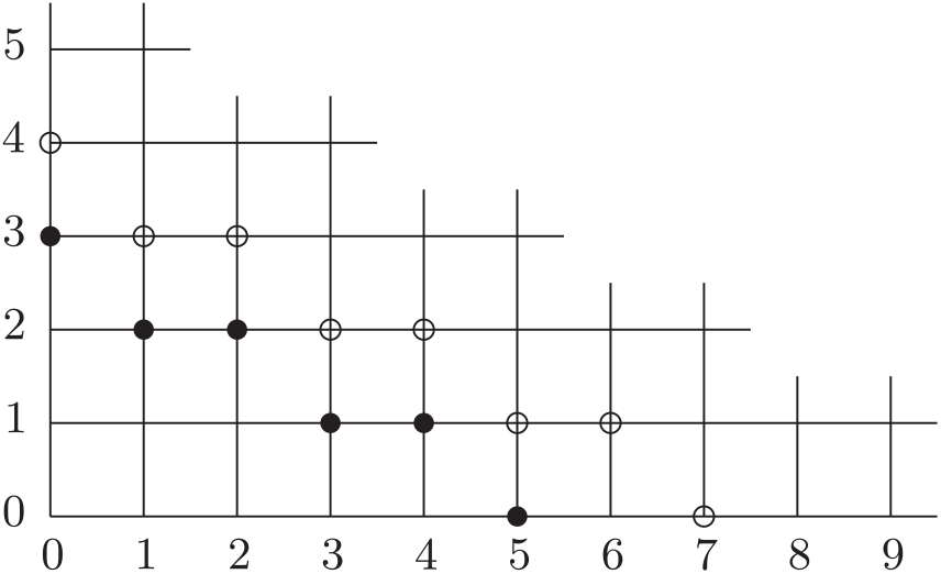
In the case
 $n=2m$
with m a positive integer, consider a particle that starts at (0, 0). At each time step, it moves one unit to the right with probability p or one unit up with probability q, stopping at the first time it reaches the boundary
 $(k,m-\lfloor k/2\rfloor)$
,
 $k=0,1,\ldots,2m$
. Let
 $Z_{2m}$
denote the x-coordinate of its final position. Then
 \begin{equation}
\mathrm{P}(Z_{2m}=k)=\binom{m + \lfloor k/2\rfloor}{k}p^k q^{m - \lfloor k/2\rfloor},\qquad k=0,1,\ldots,2m.
\end{equation}
Each lattice path ending at
 $(k,m - \lfloor k/2\rfloor)$
has probability
 $p^k q^{m - \lfloor k/2\rfloor}$
, and the binomial coefficient counts the number of paths that end at
 $(k,m-k/2)$
if k is even, and at
 $(k,m-(k-1)/2)$
if k is odd, because in the latter case the path must first reach
 $(k,m-(k+1)/2)$
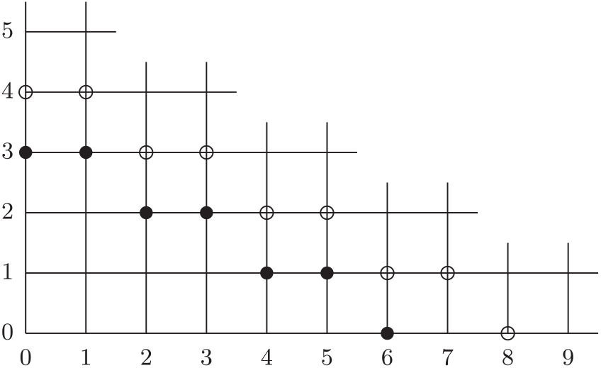
. See Figure 2.
The solid dots determine the boundary characterizing
 $Z_6$
, whereas the open dots determine the boundary characterizing
 $Z_8$
.

In the case
 $n=2m-1$
with m a positive integer, again consider a particle that starts at (0, 0). At each time step, it moves one unit to the right with probability p or one unit up with probability q, stopping at the first time it reaches the boundary
 $(k,m-\lceil k/2\rceil)$
,
 $k=0,1,\ldots,2m-1$
. Let
 $Z_{2m-1}$
denote the x-coordinate of its final position. Then
 \begin{equation}
\mathrm{P}(Z_{2m-1}=k)=\binom{m - 1 + \lceil k/2\rceil}{k}p^k q^{m - \lceil k/2\rceil},\qquad k=0,1,\ldots,2m-1.
\end{equation}
Each lattice path ending at
 $(k,m - \lceil k/2\rceil)$
has probability
 $p^k q^{m - \lceil k/2\rceil}$
, and the binomial coefficient counts the number of paths that end at
 $(k,m-(k+1)/2)$
if k is odd, and at
 $(k,m-k/2)$
if k is even, because in the latter case the path must first reach
 $(k,m-1-k/2)$
. See Figure 3.
The solid dots determine the boundary characterizing
 $Z_5$
, whereas the open dots determine the boundary characterizing
 $Z_7$
.

One observation follows immediately. Notice that, in the definitions, if the boundary were replaced by
 $(k,n-k)$
,
 $k=0,1,\ldots,n$
, then
 $Z_n$
would have the binomial(n, p) distribution. But the actual boundary, as defined above, lies on or below this one, so we conclude that
 $Z_n$
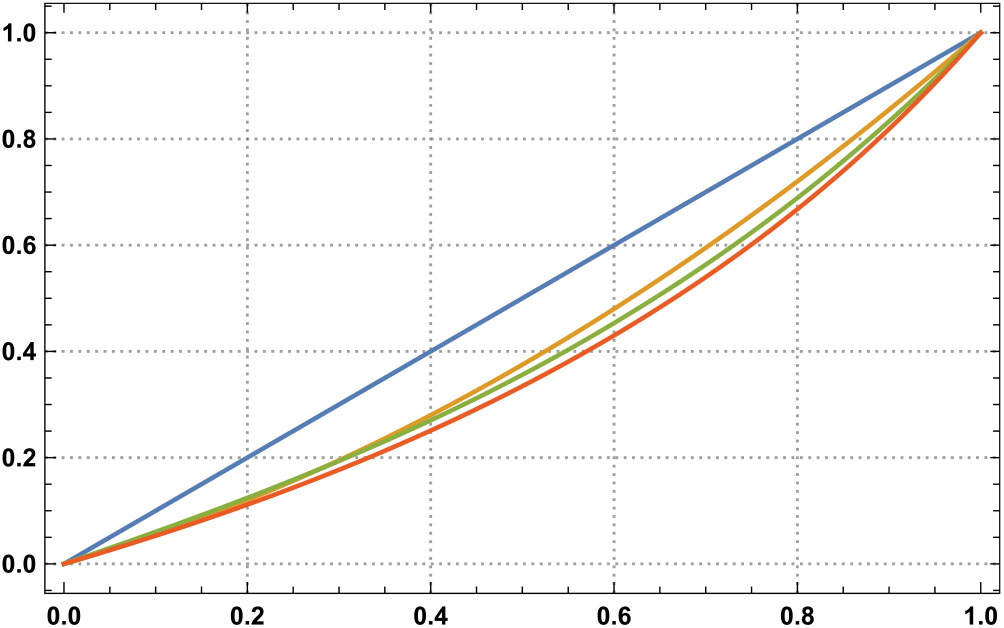
, as defined above, is stochastically less than a binomial(n, p) random variable. This suggests a potential name for our unnamed distribution: the sub-binomial distribution. Visual support for this name is provided by Figure 4 below.
 \begin{equation}
\mathrm{P}(Z_n\ \textit{is even})=\begin{cases}(1+q^{n+1})/(1+q)&\textit{if n is even},\\
(q+q^{n+1})/(1+q)&\textit{if n is odd}.\end{cases}
\end{equation}
Equivalently,
 \begin{equation*}
\mathrm{P}(Z_n\textit{ is odd})=\begin{cases}(q-q^{n+1})/(1+q)&\textit{if n is even},\\
(1-q^{n+1})/(1+q)&\textit{if n is odd}.\end{cases}
\end{equation*}
Proof.It suffices to give separate proofs for n even and n odd, both by induction. To initialize, in the
 $n=1$
case the probability mass function is q at 0 and p at 1, so (22) holds. In the
 $n=2$
case, the probability mass function is q at 0, pq at 1, and
 $p^2$
at 2, so again (22) holds.
Now assume that (22) holds for
 $n=2m$
. We must show that it holds for
 $n=2m+2$
. By the interpretation of the distribution (see Figure 2),
 \begin{align*}
\mathrm{P}(Z_{2m+2}\ \text{is even}\mid Z_{2m}\ \text{is even})&=q+p^2=1-q+q^2,\\
\mathrm{P}(Z_{2m+2}\ \text{is even}\mid Z_{2m}\ \text{is odd})&=p=1-q.
\end{align*}
We conclude that
 \begin{align*}
\mathrm{P}(Z_{2m+2}\text{ is even})&=\mathrm{P}(Z_{2m}\text{ is even})\mathrm{P}(Z_{2m+2}\text{ is even}\mid Z_{2m}\text{ is even})\\
&\quad{}+\mathrm{P}(Z_{2m}\text{ is odd})\mathrm{P}(Z_{2m+2}\text{ is even}\mid Z_{2m}\text{ is odd})\\
&=\frac{1+q^{2m+1}}{1+q}\,(1-q+q^2)+\frac{q-q^{2m+1}}{1+q}\,(1-q)\\
&=\frac{1+q^{2m+3}}{1+q},
\end{align*}
proving the lemma when n is even.
The proof when n is odd is similar, using Figure 3 in place of Figure 2, and is left to the reader.
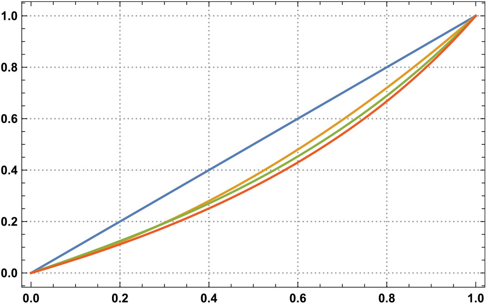
Plot of
 $f_n(p):= \mathrm{E}[Z_n]/n$
as a function of p for
 $n=1$
(blue curve),
 $n=2$
(orange curve),
 $n=5$
(green curve), and
 $n=100$
(red curve). Alternatively,
 $\frac12=f_1(\frac12)>f_2(\frac12)>f_5(\frac12)>f_{100}(\frac12)>\frac13$
if color is unavailable.
 \begin{equation*}
\textrm{E}[Z_n]=n\,\frac{p}{2-p}+[1-(-1)^n(1-p)^n]\,\frac{p(1-p)}{(2-p)^2}.
\end{equation*}
Equivalently,
 \begin{equation}
\mathrm{E}[Z_n]=n\,\frac{1-q}{1+q}+[1-(-1)^n q^n]\,\frac{q(1-q)}{(1+q)^2}.
\end{equation}
Proof.As with Lemma 1, it suffices to give separate proofs for n even and n odd, both by induction. To initialize, in the
 $n=1$
case the probability mass function is q at 0 and p at 1, so the mean is
 $p=1-q$
and (23) holds. In the
 $n=2$
case, the probability mass function is q at 0, pq at 1, and
 $p^2$
at 2, so the mean is
 $pq+2p^2=(1-q)(2-q)$
and again (23) holds.
Now assume that (23) holds for
 $n=2m$
. We must show that it holds for
 $n=2m+2$
. By the interpretation of the distribution (see Figure 2),
 \begin{align*}
\mathrm{E}[Z_{2m+2}-Z_{2m}\mid Z_{2m}\text{ is even}]&=pq+2p^2=(1-q)(2-q),\\
\mathrm{E}[Z_{2m+2}-Z_{2m}\mid Z_{2m}\text{ is odd}]&=p=1-q.
\end{align*}
We conclude from the induction hypothesis and Lemma 1 that
 \begin{align*}
\mathrm{E}[Z_{2m+2}]&=\mathrm{E}[Z_{2m}]+\mathrm{P}(Z_{2m}\text{ is even})\mathrm{E}[Z_{2m+2}-Z_{2m}\mid Z_{2m}\text{ is even}]\\
&
\quad{}+\mathrm{P}(Z_{2m}\text{ is odd})\mathrm{E}[Z_{2m+2}-Z_{2m}\mid Z_{2m}\text{ is odd}]\\
&=2m\,\frac{1-q}{1+q}+(1-q^{2m})\,\frac{q(1-q)}{(1+q)^2}\\
&\quad{}+\frac{1+q^{2m+1}}{1+q}\,(1-q)(2-q)+\frac{q-q^{2m+1}}{1+q}\,(1-q)\\
&=(2m+2)\,\frac{1-q}{1+q}+(1-q^{2m+2})\,\frac{q(1-q)}{(1+q)^2},
\end{align*}
proving the lemma when n is even.
Again, the proof when n is odd is similar, using Figure 3 in place of Figure 2, and is left to the reader.
We conclude this section with alternative interpretations of the distribution of
 $Z_n$
, given by (20) if
 $n=2m$
and by (21) if
 $n=2m-1$
, that do not require separate formulations for n even and n odd.
• Consider a particle that starts at (0, 0). At each time step, it moves one unit to the right with probability p or one unit up with probability q, stopping at the first time it reaches or crosses the boundary
$(k,(n-k)/2)$
,
$k=0,1,\ldots,n$
. Let
$Z_n$
denote the x-coordinate of its final position.• Consider a particle that starts at (0, 0). At each time step, it moves one unit to the right with probability p or two units up with probability q, stopping at the first time it reaches or crosses the boundary
$(k,n-k)$
,
$k=0,1,\ldots,n$
. Let
$Z_n$
denote the x-coordinate of its final position.• Consider a particle that starts at (0, 0). At each time step, it moves one unit to the right with probability p or one unit up with probability q followed by another unit up with probability 1, stopping at the first time it reaches the boundary
$(k,n-k)$
,
$k=0,1,\ldots,n$
. Let
$Z_n$
denote the x-coordinate of its final position.









The last of these interpretations is the context in which the distribution arises in Section 4 below.
4. Proofs of Theorems 1 and 2
Proof of Theorem
1. The result is immediate from Theorem 2 provided we can show that
 $f(\rho):= \mu(r,\rho,(AB)^s B^{r-2})$
is continuous at 0. We use Theorem 3, 5, or 6 to evaluate
 $f(\rho)$
, which is a rational function of
 $\rho$
. The only potential singularities are those of the stationary distribution
 $\boldsymbol{\pi}$
(or
 $\boldsymbol{\pi}_1$
or
 $\boldsymbol{\pi}_2$
). But the existence and uniqueness of
 $\boldsymbol{\pi}$
(or
 $\boldsymbol{\pi}_1$
or
 $\boldsymbol{\pi}_2$
) for
 $0\le\rho<1$
(see also Theorem 4) ensures that
 $f(\rho)$
is real analytic there, hence continuous.
We give two proofs of Theorem 2, the first one direct (depending solely on Theorems 4 and 5) but complicated, and the second one more easily understood but depending on Theorems 4 and 5 and Lemmas 1 and 2.
First proof of Theorem 2.First, assume that
 $r\ge3$
is odd. Since
 $\dot{{\textbf{\textit{P}}}}_A {\boldsymbol{1}}={\textbf{{0}}}$
, Theorem 4 tells us that the rate of profit, regardless of the initial capital, can be expressed as
 \begin{align}
&\mu(r,0,(AB)^sB^{r-2})\nonumber\\
&\quad{}=(2s+r-2)^{-1} \boldsymbol{\pi} \bigg[ \sum_{j=0}^{s-1}({\textbf{\textit{P}}}_A {\textbf{\textit{P}}}_B)^{\,j}{\textbf{\textit{P}}}_A \dot{{\textbf{\textit{P}}}}_B + \sum_{i=0}^{r-3}({\textbf{\textit{P}}}_A {\textbf{\textit{P}}}_B)^s ({\textbf{\textit{P}}}_B)^i\dot{{\textbf{\textit{P}}}}_B \bigg]{\boldsymbol{1}},
\end{align}
where
 $\boldsymbol{\pi}$
is the stationary distribution of
 ${\textbf{\textit{P}}}:= ({\textbf{\textit{P}}}_A {\textbf{\textit{P}}}_B)^s ({{\textbf{\textit{P}}}}_B)^{r-2}$
. Since
 $\rho=0$
and r is odd,
 ${\textbf{\textit{P}}}$
is reducible with one recurrent class
 $\{0, r-1\}$
and
 $r-2$
transient states. From the observations about the pattern
 $(AB)^sB^{r-2}$
in Section 1 it follows that
 ${\textbf{\textit{P}}}(0,0)=1-{\textbf{\textit{P}}}(0,r-1)=1-2^{-s}$
and
 ${\textbf{\textit{P}}}(r-1,0)=1$
, so that the stationary distribution
 $\boldsymbol{\pi}$
is given by
 $\boldsymbol{\pi}=(\pi_0, 0, 0, \ldots, 0, \pi_{r-1})$
, where
 \begin{align*}
\pi_0 = 1- \pi_{r-1}= \frac{2^s}{2^s+1}.
\end{align*}
Except for the factor
 $(2s+r-2)^{-1}$
, all of the terms in (24) have the form
 $\boldsymbol{\pi}\boldsymbol{\Lambda}\dot{{\textbf{\textit{P}}}}_B{\boldsymbol{1}}$
for a transition matrix
 ${\boldsymbol{\Lambda}}=(\lambda_{i,j})_{i,j=0,1,\ldots,r-1}$
. Therefore, using
 $\dot{{\textbf{\textit{P}}}}_B{\boldsymbol{1}}=(-1,1,1,\ldots,1)^\top$
, we have
 \begin{equation}
\boldsymbol{\pi}\boldsymbol{\Lambda}\dot{{\textbf{\textit{P}}}}_B{\boldsymbol{1}}=1-2(\pi_0 \lambda_{0,0}+\pi_{r-1}\lambda_{r-1,0}),
\end{equation}
showing that we need only determine two of the entries of
 $\boldsymbol{\Lambda}$
to evaluate (25).
We first consider the transition matrix
 $\boldsymbol{\Lambda}=({\textbf{\textit{P}}}_A {\textbf{\textit{P}}}_B)^{\,j}{\textbf{\textit{P}}}_A$
for
 $0\leq j\leq s-1$
. When
 $j<(r-1)/2$
, we have
 $\lambda_{0,0}=0$
. When
 $j\geq(r-1)/2$
, from state 0 we can reach state
 $r-1$
after j plays of AB if there are at least
 $(r-1)/2$
wins from the j plays of game A, after which we can move to state 0 with an additional win from game A. Thus, we have
 \begin{align*}
\lambda_{0,0}=\sum_{k=(r-1)/2}^{\,j} \binom{j}{k}\frac{1}{2^{\,j+1}}.
\end{align*}
For all j, we have
 $\lambda_{r-1,0}=1/2$
. Using (25), for
 $j<(r-1)/2$
,
 \begin{align*}
\boldsymbol{\pi} ({\textbf{\textit{P}}}_A {\textbf{\textit{P}}}_B)^{\,j}{\textbf{\textit{P}}}_A \dot{{\textbf{\textit{P}}}}_B {\boldsymbol{1}}=1-2\pi_{r-1}\,\frac12 = \pi_0 = \frac{2^s}{2^s+1},
\end{align*}
and for
 $j\geq(r-1)/2$
,
 \begin{align*}
\boldsymbol{\pi} ({\textbf{\textit{P}}}_A {\textbf{\textit{P}}}_B)^{\,j} {\textbf{\textit{P}}}_A \dot{{\textbf{\textit{P}}}}_B {\boldsymbol{1}} &= 1-2\bigg[\pi_0 \sum_{k=(r-1)/2}^{\,j} \binom{j}{k}\frac{1}{2^{\,j+1}} + \pi_{r-1}\,\frac12\bigg] \\
&= \frac{2^s}{2^s+1}\bigg[1-\sum_{k=(r-1)/2}^{\,j} \binom{j}{k}\frac{1}{2^{\,j}}\bigg].
\end{align*}
Summing these s terms, we have
 \begin{align}
\sum_{j=0}^{s-1}\boldsymbol{\pi} ({\textbf{\textit{P}}}_A {\textbf{\textit{P}}}_B)^{\,j}{\textbf{\textit{P}}}_A \dot{{\textbf{\textit{P}}}}_B {\boldsymbol{1}}=
\frac{2^s}{2^s+1}\bigg[s - \sum_{j=(r-1)/2}^{s-1}\;\sum_{k=(r-1)/2}^{\,j} \binom{j}{k} \frac{1}{2^{\,j}}\bigg].
\end{align}
Next we consider the transition matrix
 $\boldsymbol{\Lambda}=({\textbf{\textit{P}}}_A {\textbf{\textit{P}}}_B)^s({\textbf{\textit{P}}}_B)^i$
for
 $0\leq i\leq r-3$
. For even i, we have
 $\lambda_{0,0}= 2^{-s}$
and
 $\lambda_{r-1,0}=0$
, from which we obtain, via (25),
 \begin{align*}
\boldsymbol{\pi} ({\textbf{\textit{P}}}_A {\textbf{\textit{P}}}_B)^s({\textbf{\textit{P}}}_B)^i \dot{{\textbf{\textit{P}}}}_B {\boldsymbol{1}}=1-2\pi_0\,2^{-s} = \frac{2^s -1}{2^s+1}.
\end{align*}
Now let i be odd. Assume we start from state 0. With at least
 $(r-i)/2$
wins from s plays of game A, we can reach state
 $r-i$
or an even state to its right after s plays of game AB, and then move to state 0 after i additional plays of game B. Thus, we have
 \begin{align*}
\lambda_{0,0}=\sum_{k=(r-i)/2}^s \binom{s}{k}\frac{1}{2^s}.
\end{align*}
Moreover,
 $\lambda_{r-1, 0}= 1$
. Thus, for odd i we obtain, via (25),
 \begin{align*}
\boldsymbol{\pi} ({\textbf{\textit{P}}}_A {\textbf{\textit{P}}}_B)^s({\textbf{\textit{P}}}_B)^i \dot{{\textbf{\textit{P}}}}_B {\boldsymbol{1}}&=1-2\bigg[\pi_0 \sum_{k=(r-i)/2}^s \binom{s}{k} \frac{1}{2^s}+\pi_{r-1}\bigg] \\
&=\frac{2^s-1}{2^s+1}-\frac{2}{2^s+1}\sum_{k=(r-i)/2}^s \binom{s}{k}.
\end{align*}
Summing over i, we have
 \begin{equation}
\sum_{i=0}^{r-3}\boldsymbol{\pi} ({\textbf{\textit{P}}}_A {\textbf{\textit{P}}}_B)^s({\textbf{\textit{P}}}_B)^i \dot{{\textbf{\textit{P}}}}_B {\boldsymbol{1}}=
(r-2)\frac{2^s-1}{2^s+1}-\frac{2}{2^s+1}\sum_{i=1}^{(r-3)/2}\!\!\!\sum_{k=(r-2i+1)/2}^s \binom{s}{k}.
\end{equation}
For the double sum in (27), a change of variables gives
 \begin{equation*}
\sum_{i=1}^{(r-3)/2}\sum_{k=(r-2i+1)/2}^s \binom{s}{k}=\sum_{j=2}^{(r-1)/2}\sum_{k=j}^s \binom{s}{k}.
\end{equation*}
There are two cases. If
 $(r-1)/2\ge s$
, which also makes the double sum in (26) zero, then this becomes
 \begin{align}
\sum_{j=2}^s\sum_{k=j}^s \binom{s}{k}&=\sum_{k=2}^s\sum_{j=2}^k\binom{s}{k}=\sum_{k=2}^s(k-1)\binom{s}{k}=\sum_{k=0}^s(k-1)\binom{s}{k}+1\nonumber\\
&=s2^{s-1}-2^s+1=\frac{s2^s-2(2^s-1)}{2},
\end{align}
and (24) becomes
 \begin{align*}
\mu(r,0,(AB)^sB^{r-2})&=\frac{1}{2s+r-2}\bigg[\frac{s2^s}{2^s+1}+(r-2)\frac{2^s-1}{2^s+1}-\frac{s2^s-2(2^s-1)}{2^s+1}\bigg]\nonumber\\
&=\frac{r}{2s+r-2}\,\frac{2^s-1}{2^s+1}.
\end{align*}
If
 $(r-1)/2<s$
, it suffices to verify the following identity:
 \begin{align*}
\sum_{j=(r-1)/2}^{s-1}\sum_{k=(r-1)/2}^{\,j}\binom{j}{k} 2^{s-j}+2\sum_{j=2}^{(r-1)/2}\sum_{k=j}^s\binom{s}{k}=s2^s-2(2^s-1).
\end{align*}
For
 $1\le s_0<s$
,
 \begin{align*}
&\sum_{j=s_0}^{s-1}\sum_{k=s_0}^{\,j}\binom{j}{k}2^{s-j}+2\sum_{j=2}^{s_0}\sum_{k=j}^s\binom{s}{k}-[s2^s-2(2^s-1)]\\
&\qquad{}=\sum_{j=s_0}^{s-1}\sum_{k=s_0}^{\,j}\binom{j}{k}2^{s-j}-2\sum_{j=s_0+1}^{s}\sum_{k=j}^s\binom{s}{k}\\
&\qquad{}=\sum_{k=s_0}^{s-1}\sum_{j=k}^{s-1}\binom{j}{k}2^{s-j}-2\sum_{k=s_0+1}^s\sum_{j=k}^s\binom{s}{j}\\
&\qquad{}=\sum_{k=s_0+1}^{s} 2^{s+1}\bigg[\sum_{j=k-1}^{s-1}\binom{j}{k-1}\frac{1}{2^{\,j+1}}-\sum_{j=k}^s\binom{s}{j}\frac{1}{2^s}\bigg]\\
&\qquad{}=0,
\end{align*}
where the first equality uses (28) and the last equality uses the relationship between the binomial and negative binomial distributions. (The first sum within brackets is the probability that, in a sequence of independent Bernoulli trials with success probability
 $1/2$
, at most s trials are needed for the kth success, and the second sum is the probability that at least k successes occur in s trials.)
Next, assume that
 $r\ge4$
is even. Theorem 5 tells us that the rate of profit can be expressed as
 \begin{align}
&\mu(r,0,(AB)^sB^{r-2})\nonumber\\
&\quad{}=(2s+r-2)^{-1} \boldsymbol{\pi}_0\bigg[ \sum_{j=0}^{s-1}({\textbf{\textit{P}}}_A {\textbf{\textit{P}}}_B)^{\,j}{\textbf{\textit{P}}}_A \dot{{\textbf{\textit{P}}}}_B + \sum_{i=0}^{r-3}({\textbf{\textit{P}}}_A {\textbf{\textit{P}}}_B)^s ({\textbf{\textit{P}}}_B)^i\dot{{\textbf{\textit{P}}}}_B \bigg]{\boldsymbol{1}},
\end{align}
where
 $\boldsymbol{\pi}_0:= (1,0,0,\ldots,0)$
if the initial capital is even and
 $\boldsymbol{\pi}_0:= (0,0,\ldots,0,1)$
if the initial capital is odd.
Except for the factor
 $(2s+r-2)^{-1}$
, all of the terms in (29) have the form
 $\boldsymbol{\pi}_0\boldsymbol{\Lambda}\dot{{\textbf{\textit{P}}}}_B{\boldsymbol{1}}$
for a transition matrix
 ${\boldsymbol{\Lambda}}=(\lambda_{i,j})_{i,j=0,1,\ldots,r-1}$
, and
 \begin{equation*}
\boldsymbol{\pi}_0\boldsymbol{\Lambda}\dot{{\textbf{\textit{P}}}}_B{\boldsymbol{1}}=\begin{cases}1-2\lambda_{0,0}&\text{if initial capital is even},\\1-2\lambda_{r-1,0}&\text{if initial capital is odd}.\end{cases}
\end{equation*}
For
 $\boldsymbol{\Lambda}=({\textbf{\textit{P}}}_A{\textbf{\textit{P}}}_B)^{\,j}{\textbf{\textit{P}}}_A$
with
 $0\le j\le s-1$
,
 $\lambda_{0,0}=0$
and
 $\lambda_{r-1,0}=1/2$
. For
 $\boldsymbol{\Lambda}=({\textbf{\textit{P}}}_A{\textbf{\textit{P}}}_B)^s({\textbf{\textit{P}}}_B)^i$
with
 $0\le i\le r-3$
,
 $\lambda_{0,0}=0$
if i is odd and
 \begin{equation*}
\lambda_{0,0}=\bigg[\binom{s}{0}+\sum_{m=1}^{\lceil 2s/r\rceil}\sum_{k=(mr-i)/2}^{mr/2}\binom{s}{k}\bigg]\frac{1}{2^s}\end{equation*}
if i is even. Finally,
 $\lambda_{r-1,0}=1$
if i is odd and
 $\lambda_{r-1,0}=0$
if i is even.
Therefore, if the initial capital is odd,
 \begin{equation*}
\mu(r,0,(AB)^s B^{r-2})=\frac{1}{2s+r-2}\bigg[s\bigg(1-2\cdot\frac12\bigg)+\frac{r-2}{2}\,(1-1)\bigg]=0,\end{equation*}
and if the initial capital is even,
 \begin{align*}
&\mu(r,0,(AB)^s B^{r-2})\\
&\qquad{}=\frac{1}{2s+r-2}\bigg\{s+r-2-2\sum_{i=0}^{r/2-2}\bigg[\binom{s}{0}+\sum_{m=1}^{\lceil 2s/r\rceil}\;\sum_{k=mr/2-i}^{mr/2}\binom{s}{k}\bigg]\frac{1}{2^s}\bigg\}.
\end{align*}
It remains to check that this last expression coincides with the formula in (11). The quantity within braces is equal to
 \begin{array}{*{20}{c}}
{} \hfill & {s + r - 2 - 2(\frac{r}{2} - 1)\frac{1}{{{2^s}}} - 2\sum\limits_{m = 1}^{\left\lceil {2s/r} \right\rceil } {\sum\limits_{j = (m - 1)r/2 + 2}^{mr/2} {\sum\limits_{k = j}^{mr/2} {\left( \begin{array}{c}
s \\
k \\
\end{array} \right)} } } \frac{1}{{{2^s}}}} \hfill \\
= \hfill & {s + (r - 2)(1 - \frac{1}{{{2^s}}}) - 2\sum\limits_{m = 1}^{\left\lceil {2s/r} \right\rceil } {\sum\limits_{k = (m - 1)r/2 + 2}^{mr/2} {(k - 1 - (} } m - 1)r/2)\left( \begin{array}{c}
s \\
k \\
\end{array} \right)\frac{1}{{{2^s}}}} \hfill \\
= \hfill & {s + (r - 2)(1 - \frac{1}{{{2^s}}}) - 2\sum\limits_{m = 1}^{\left\lceil {2s/r} \right\rceil } {\sum\limits_{k = (m - 1)r/2 + 1}^{mr/2} {(k - 1 - (} } m - 1)r/2)\left( \begin{array}{c}
s \\
k \\
\end{array} \right)\frac{1}{{{2^s}}}} \hfill \\
= \hfill & {s + (r - 2)(1 - \frac{1}{{{2^s}}}) - 2\sum\limits_{k = 0}^s {(k - 1)} \left( \begin{array}{c}
s \\
k \\
\end{array} \right)\frac{1}{{{2^s}}} - \frac{2}{{{2^s}}} + r\sum\limits_{m = 1}^{\left\lceil {2s/r} \right\rceil } {(m - 1)} \sum\limits_{k = (m - 1)r/2 + 1}^{mr/2} {\left( \begin{array}{c}
s \\
k \\
\end{array} \right)} \frac{1}{{{2^s}}}n} \hfill \\
= \hfill & {s + (r - 2)(1 - \frac{1}{{{2^s}}}) - 2(\frac{s}{2} - 1) - \frac{2}{{{2^s}}} - r(1 - \frac{1}{{{2^s}}}) + r\sum\limits_{m = 1}^{\left\lceil {2s/r} \right\rceil } m \sum\limits_{k = (m - 1)r/2 + 1}^{mr/2} {\left( \begin{array}{c}
s \\
k \\
\end{array} \right)} \frac{1}{{{2^s}}}} \hfill \\
= \hfill & {r\sum\limits_{m = 1}^{\left\lceil {2s/r} \right\rceil } m \sum\limits_{k = (m - 1)r/2 + 1}^{mr/2} {\left( \begin{array}{c}
s \\
k \\
\end{array} \right)} \frac{1}{{{2^s}}} = r{\mkern 1mu} \sum\limits_{k = 0}^s {\left\lceil {\frac{{2k}}{r}} \right\rceil } \left( \begin{array}{c}
s \\
k \\
\end{array} \right)\frac{1}{{{2^s}}},} \hfill \\
\end{array}\
and the proof is complete.
Second proof of Theorem 2.First, fix an odd integer
 $r\ge3$
and a positive integer s. We apply Theorem 4 assuming (15)–(18) with
 $\rho=0$
in (4) and
 $C_1C_2\cdots C_t=(AB)^s B^{r-2}$
with
 $t:= 2s+r-2$
, to conclude that
 \begin{equation}
\mu(r,0,(AB)^s B^{r-2})=\lim_{n\to\infty}(nt)^{-1}\mathrm{E}[S_{nt}].
\end{equation}
(The theorem tells us that the rate of profit does not depend on the initial capital, so for convenience we take the initial capital congruent to 0 (mod r).) Here,
 $S_1,S_2,\ldots$
is the player’s sequence of cumulative profits. We can evaluate
 $\mathrm{E}[S_{nt}]$
.
With
 $Z_n$
having the probability mass function in (20) if
 $n=2m$
and in (21) if
 $n=2m-1$
, we claim that
 \begin{equation*}\mathrm{P}(S_{nt}=kr-\text{mod}(n-k,2))=\mathrm{P}(Z_n=k),\qquad k=0,1,\ldots,n,\end{equation*}
if
 $p=1-2^{-s}$
. The result follows by using the third of the alternative interpretations of the distribution in (20) and (21) at the end of Section 3.
We can now evaluate, with the help of Lemmas 1 and 2, the mean cumulative profit after nt games:
 \begin{align*}
\mathrm{E}[S_{nt}]&=\sum_{k=0}^n (kr-\text{mod}(n-k,2))\mathrm{P}(Z_n=k)\\
&=r\mathrm{E}[Z_n]-\mathrm{P}(n-Z_n\text{ is odd})\\
&=r\bigg(n\,\frac{1-q}{1+q}+[1-(-1)^n q^n]\,\frac{q(1-q)}{(1+q)^2}\bigg)-\frac{q-(-1)^n q^{n+1}}{1+q}.
\end{align*}
We divide by
 $nt=n(2s+r-2)$
and let
 $n\to\infty$
to obtain
 \begin{equation*}
\lim_{n\to\infty}(nt)^{-1}\mathrm{E}[S_{nt}]=\frac{r}{2s+r-2}\,\frac{1-q}{1+q}=\frac{r}{2s+r-2}\,\frac{2^s-1}{2^s+1},\end{equation*}
so (10) follows from this and (30).
Second, fix an even integer
 $r\ge4$
and a positive integer s. We apply Theorem 5 assuming (15)–(18) with
 $\rho=0$
in (4) and
 $C_1C_2\cdots C_t=(AB)^s B^{r-2}$
with
 $t:= 2s+r-2$
, to conclude that (30) holds. (The theorem tells us that the rate of profit depends on the initial capital only through its parity, so for convenience we take the initial capital congruent to 0 (mod r) if the initial capital is even, or congruent to
 $r-1$
(mod r) if odd.) Recalling from Section 1 that, with initial capital congruent to 0 (mod r), each play of
 $(AB)^s B^{r-2}$
results in a mean profit of
 \begin{align*}
\mathrm{E}[S_t]=\sum_{m=1}^{\lceil 2s/r\rceil}mr\sum_{k=(m-1)r/2+1}^{mr/2}\binom{s}{k}\frac{1}{2^s}=r\,\sum_{k=0}^s\bigg\lceil\frac{2k}{r}\bigg\rceil\binom{s}{k}\frac{1}{2^s},
\end{align*}
we find that
 \begin{equation*}
\lim_{n\to\infty}(nt)^{-1}\mathrm{E}[S_{nt}]=\frac{r}{2s+r-2}\,\sum_{k=0}^s\bigg\lceil\frac{2k}{r}\bigg\rceil\binom{s}{k}\frac{1}{2^s}.\end{equation*}
With initial capital congruent to
 $r-1$
(mod r),
 $\mathrm{P}(S_{nt}=0)=1$
, so
 \begin{equation*}\lim_{n\to\infty}(nt)^{-1}\mathrm{E}[S_{nt}]=0,\end{equation*}
Acknowledgements
We are grateful to Derek Abbott for raising the question addressed here, to Ira Gessel for suggesting the lattice path interpretation of the distribution defined by (20) and (21), and to the editors and reviewers for help in improving the presentation. The work of S. N. Ethier was partially supported by a grant from the Simons Foundation (429675) and the work of J. Lee was supported by the Basic Science Research Program through the National Research Foundation of Korea (NRF) funded by the Ministry of Education (NRF-2018R1D1A1B07042307).