1. INTRODUCTION
In this paper we study generalized method of moments (GMM) estimation of the inclusive panel AR(1) model that contains the covariance stationary panel AR(1) model and the panel AR(1) model with a unit root as special cases.
We first derive a linear GMM (LGMM) estimator for the autoregression parameter ρ in the inclusive panel AR(1) model that exhausts all the information in the second moments of the data. We show that when |ρ| < 1 an optimal version of our LGMM estimator is asymptotically equivalent to the optimal GMM estimator for the inclusive panel AR(1) model that was proposed by Ahn and Schmidt (1997). The latter estimator exploits a moment condition that is nonlinear in ρ.
Next we derive the asymptotic distribution of the two-step optimal linear GMM (OLGMM) estimator when ρ = 1 under a variety of assumptions about the initial observations and the initial estimator. We find that this distribution is nonnormal and involves the asymptotic distribution of the initial estimator. In most cases that we consider the OLGMM estimator is superconsistent. In addition we show that the iterated OLGMM estimator is superefficient when the variance of the initial observations is finite and fixed, i.e., small compared to the cross-sectional dimension of the panel. These asymptotic properties of the OLGMM estimators are related to a moment condition that only identifies the unit root and whose sample counterpart holds deterministically when ρ = 1. As a result, this moment condition is extremely informative when ρ = 1.
We also conduct a Monte Carlo study of the finite-sample behavior of various GMM estimators for the inclusive panel AR(1) model. In the Monte Carlo study we will pay special attention to the gain in precision and reduction in the root mean squared error (RMSE) that will be achieved when ρ is close to or equal to one by employing our preferred version of the OLGMM estimator instead of other GMM estimators that use a different weight matrix and/or use fewer moment conditions, such as, e.g., the system estimator of Arellano and Bover (1995) and Blundell and Bond (1998).
The paper is organized as follows. Section 2 reviews GMM estimation of the covariance stationary panel AR(1) model. Section 3 introduces the LGMM estimator for the inclusive panel AR(1) model. Section 4 examines the asymptotic properties of the OLGMM estimator and an iterative version of this estimator. Finally, Section 5 compares the performance of various GMM estimators for the inclusive panel AR(1) model by means of a Monte Carlo study. The proofs are collected in the Appendix.
2. THE INCLUSIVE PANEL AR(1) MODEL
Consider the panel AR(1) model with random effects:


for i = 1,…, N and t = S + 1,…,T, where S ≤ 1 is the common starting date of the N processes. We assume that the number of “individuals” in the panel, N, is large and the number of observations per individual, T, is fixed. Moreover −1 < ρ ≤ 1.
The observations on y = (y.,1… y.,T)′ are independent and identically distributed (i.i.d.) across the N individuals.1
We assume identical distributions across the individuals for convenience.


and

We also assume that the idiosyncratic errors, the εi,t, are homoskedastic over time:

Finally, the initial conditions are given by yi,S = μi + (1 − ρ)ξi,S, where Var(ξi,S) < ∞, for i = 1,…, N. Note that when ρ = 1 the initial conditions are equal to the individual effects, the μi.
When |ρ| < 1, we assume that {yi,t} is covariance stationary. Ahn and Schmidt (1997) have shown that given assumptions (3)–(7), {yi,t} is covariance stationary if and only if the initial observations satisfy the following assumptions:


The first assumption, (8), is also known as mean-stationarity (cf. Arellano and Bover, 1995; Blundell and Bond, 1998).
When ρ = 1, we have

for i = 1,…, N. It follows that in this case E(yi,1) = E(μi) also. Therefore, when ρ = 1, E(yi,1) = 0 and σ12 = Var(yi,12) = E(yi,12) = σμ2 + (1 − S)σ2. In the asymptotic analysis we allow 1 − S and thereby σ12 to be related to N. That is, in the unit root case we assume that

where σ12 is a constant and 0 ≤ b ≤ ½. The parameter b determines the relation between σ12 and N. If the {yi,t} actually began close to the date of the first observation and σ12/σ2 is not very large whereas N is large, then b is approximately zero; however, if the {yi,t} began a long time before t = 1 so that σ12/σ2 is large whereas N is not very large, then it is more reasonable to assume that b is closer to ½.
We are now able to give a formal definition of the inclusive panel AR(1) model.
DEFINITION 1. The inclusive panel AR(1) model with random effects is characterized by (1) and (2), Assumptions (3)–(7), and either Assumptions (8) and (9) when |ρ| < 1 or Assumption (10) when ρ = 1.
If we restrict the parameter space to |ρ| < 1, we obtain the covariance stationary panel AR(1) model with random effects.
2.1. Moment Conditions for the Covariance Stationary Panel AR(1) Model
We will review all the moment conditions that are available for GMM estimation of the covariance stationary panel AR(1) model with random effects.
Arellano and Bond (1991) have derived the following (T − 1)(T − 2)/2 basic moment conditions from Assumptions (4)–(6):

where Δvi,t = vi,t − vi,t−1.
If mean-stationarity, (8), holds too, we can add T − 2 moment conditions to the basic moment conditions (see Arellano and Bover, 1995):

The estimator that exploits the moment conditions in both (11) and (12) is known as the system (SYS) estimator.
Adding the assumption of homoskedasticity, (7), implies another T − 2 moment conditions (see Ahn and Schmidt, 1995):

Notice that all the preceding moment conditions are linear in ρ.
Finally, adding the “covariance stationarity assumption” (9) yields one more moment condition (see Ahn and Schmidt, 1997):2
Covariance stationarity of {yi,t} also implies restrictions on first moments: E(Δyi,t) = 0, t = 2,…,T. However, they do not contain any information on ρ.

Notice that this moment condition is nonlinear in ρ. Therefore, computing the value of the GMM estimator of Ahn and Schmidt (1997) for the covariance stationary panel AR(1) model, which exploits all the moment conditions in (11)–(14), requires numerical optimization.
3. AN EFFICIENT LGMM ESTIMATOR FOR THE COVARIANCE STATIONARY PANEL AR(1) MODEL
We define the LGMM estimator for ρ in the covariance stationary panel AR(1) model as the estimator that exploits the T(T + 1)/2 − 3 moment conditions specified in (11)–(13), which are all linear in ρ, and a new moment condition, which is implied by covariance stationarity of {yi,t}:

Notice that this moment condition is also linear in ρ. Thus the LGMM estimator exploits (15) instead of the nonlinear moment condition (14) but otherwise exploits the same moment conditions as the Ahn–Schmidt estimator for ρ in the covariance stationary panel AR(1) model.
We have the following result.
THEOREM 1. The two-step OLGMM estimator and the two-step optimal Ahn–Schmidt GMM estimator for the covariance stationary panel AR(1) model are asymptotically equivalent.
It should be noted that there is no feasible one-step optimal weight matrix for the moment conditions exploited by these estimators.
Clearly, the LGMM estimator is more easily calculated than the nonlinear GMM estimator due to Ahn and Schmidt, and its properties are more easily investigated. For instance, under normality it can easily be shown that (15) is not redundant relative to the moment conditions specified in (11)–(13) when an optimal weight matrix is used. Using arguments similar to those in Ahn and Schmidt (1995), it can also easily be shown that the OLGMM estimator attains the semiparametric efficiency lower bound for the stationary panel AR(1) model with random effects. Moreover, under normality, the OLGMM estimator is asymptotically equivalent to the random effects maximum likelihood estimator (MLE) for ρ in the stationary panel AR(1) model and attains the Cramér–Rao (CR) lower bound when |ρ| < 1. We will see in Section 4 that the LGMM estimator also exists for ρ = 1, unlike the random effects MLE.
As a computationally simpler alternative to their nonlinear estimator, Ahn and Schmidt (1997) proposed a linearized version of their estimator. The optimal version of this estimator is given by

, where

is an initial

-consistent estimator for ρ,

is the vector of sample moment conditions,

, and

. The OLGMM estimator and the optimal linear Ahn and Schmidt GMM (OLASGMM) estimator are asymptotically equivalent when |ρ| < 1 but have different finite-sample properties.
4. ASYMPTOTIC PROPERTIES OF THE OLGMM ESTIMATOR WHEN ρ = 1
We first note some properties of the moment conditions that are implied by the inclusive panel AR(1) model when ρ = 1. Without loss of generality we assume that T = 3. Then each of (11)–(13) contains exactly one moment condition, and the covariance stationary panel AR(1) model implies a total of four moment conditions that depend only on ρ:

Let m(ρ) = (m1(ρ), m2(ρ), m3(ρ), m4(ρ))′. The moment conditions in E(m(ρ)) = 0 are also valid for ρ = 1. We have the following result on identification when ρ = 1 (cf. Arellano and Bover, 1995).
LEMMA 2. All the moment conditions that are exploited by the LGMM estimator identify the unit root except for the moment conditions due to Arellano and Bond (1991) given in (11).
However, some elements of the vector E(dm(ρ)/dρ) are discontinuous at ρ = 1.
LEMMA 3. Let {yi,t} satisfy the inclusive model. Then limρ↑1 E(dm(ρ)/dρ) ≠ E(dm(ρ)/dρ|ρ=1).
We will see subsequently that the discontinuity of E(dm(ρ)/dρ) accounts for the discontinuity of the asymptotic distributions of the OLGMM estimator and the SYS estimator at ρ = 1.
Let us now consider p4(ρ) = 2m2(ρ) + m4(ρ) = (1 − ρ)(yi,22 − yi,12). Because p4(ρ) is a linear combination of m2(ρ) and m4(ρ), it must be true that E(p4(ρ)) = 0 for −1 < ρ ≤ 1. Indeed, when |ρ| < 1, E(p4(ρ)) = 0 due to covariance stationarity of {yi,t}. However, note that for ρ = 1, we not only have E(p4(ρ)) = 0 but as a matter of fact p4(ρ) = 0; i.e., p4(ρ) = 0 holds deterministically at ρ = 1. Moreover, E(dp4(ρ)/dρ|ρ = 1) = −E(yi,22 − yi,12|ρ = 1) = −σ2 ≠ 0. Therefore, when ρ = 1, an estimator that gives all weight to E(p4(ρ)) = 0 would be an optimal GMM estimator for ρ. The value of such an estimator equals one with probability one. However, when |ρ| < 1, E(dp4(ρ)/dρ) = 0, and therefore a GMM estimator that only exploits E(p4(ρ)) = 0 would be inconsistent in this case. Nevertheless, GMM estimators that combine E(p4(ρ)) = 0 with (some) other linearly independent moment condition(s) contained in E(m(ρ)) = 0 are consistent for both |ρ| < 1 and ρ = 1. It follows that one can construct a GMM estimator for ρ that is consistent for −1 < ρ ≤ 1 and has an arbitrarily small asymptotic variance when ρ = 1 by choosing the weight for E(p4(ρ)) = 0 sufficiently high relative to the weight given to other moment conditions. In particular, there exist GMM estimators for ρ that have an asymptotic variance that is smaller than the CR lower bound for ρ = 1 (which is given in the proof of Corollary 5). Such estimators are known as superefficient estimators. We will see that the iterated OLGMM estimator (cf. Hansen, Heaton, and Yaron, 1996) is a superefficient estimator when ρ = 1 and b = 0, i.e., σ12 = E(yi,12) = σ12.
We now consider the asymptotic distribution of the OLGMM estimator when ρ = 1. We first note that the set of moment conditions contained in E(m(ρ)) = 0 is equivalent to the set of moment conditions contained in E(p(ρ)) = 0, where p(ρ) = [p1(ρ), p2(ρ), p3(ρ), p4(ρ)]′ = [m1(ρ)/σ1, m2(ρ), m3(ρ) − m1(ρ), p4(ρ)]′. We have scaled m1(ρ) by σ1 to guarantee that

converges in distribution regardless of our assumption about σ1, i.e., about the value of b. We let

denote an initial Na-consistent estimator for ρ that can be used to construct the asymptotically optimal weight matrix for the LGMM estimator:

, with a ≥ ½ and

. Examples of estimators that can be used as initial estimators for ρ are the SYS estimator and the first difference MLE for the inclusive panel AR(1) model. Note that b ≤ a. Finally, we strengthen the assumptions made in Section 2 by including the following additional assumptions.


These additional assumptions are stronger than necessary but made for convenience. Let

. Then we have the following result.
THEOREM 4. Let ρ = 1 and T = 3. Then

and

, where

and

are given in Lemmas 6 and 7 in the Appendix, respectively. Here

and

. Furthermore, if b < ½, then

, whereas if b = ½, then

. Finally, if b < a, then

, whereas if b = a = ½, then

, where the values of the elements of

depend on the values of a and b. There are three cases: b = 0, 0 < b < a, and b = a. The values of the elements of

in these cases are implicitly given in the proof of Lemma 8 in the Appendix.
Note that the asymptotic distribution of the OLGMM estimator depends on the asymptotic distribution of

, i.e., on

, whatever the values of a and b.
When ρ = 1 and b < a, the OLGMM estimator is superconsistent. In addition, we have the following result for the iterated OLGMM estimator.
COROLLARY 5. When ρ = 1 and b = 0, the iterated OLGMM estimator is superefficient.
When 0 < b < ½, the iterated OLGMM estimator is not superefficient because in this case not only does the asymptotic variance of the iterated OLGMM estimator tend to zero when the number of iterations goes to infinity but also the CR lower bound tends to zero because limN→∞ E(yi,12) = ∞ when b > 0.
When ρ = 1 and b < a, it follows from Lemma 8 and the fact that limN→∞ Nb−a = 0 that

for k = 1,2,3,4.
3Note however that E(p4(ρ)) = 0 is not redundant (otherwise E(p4(ρ)) = 0 should be dropped). On the contrary, p4(ρ) = 0 holds deterministically at ρ = 1 and only at ρ = 1 (so that Var(p4(1)) = 0). Therefore E(p4(ρ)) = 0 is extremely informative when ρ = 1 and should receive maximal weight rather than zero weight when ρ = 1.

, gives in principle all weight to E(p4(ρ)) = 0 when ρ = 1 and b < a. Hence

with

when b < ½, and

when b = ½. However, because p4,i(1) = 0 and hence

, the first three elements of

still enter the asymptotic distribution of the OLGMM estimator when b < a, i.e.,

.
When ρ = 1 and b = a = ½, the weight matrix

is no longer asymptotically optimal because it also gives weight to moment conditions other than E(p4(ρ)) = 0. This is a consequence of the fact that it makes use of an initial estimator of ρ, i.e.,

, rather than its true value.
4The weight matrix

would still be asymptotically optimal for ρ = 1 when b = a = ½. However, an estimator for ρ that uses this weight matrix would be inconsistent if |ρ| < 1.
The results stated in Lemma 8 and also the results discussed previously, notably Theorem 4 and Corollary 5, can be generalized to allow for arbitrary value of T. When T > 3 the moment conditions in E(p(ρ)) = 0 and in particular E(p4(ρ)) = 0 are still valid. However, there are T(T + 1)/2 − 6 additional moment conditions that resemble E(p1(ρ)) = 0, E(p2(ρ)) = 0, and E(p3(ρ)) = 0 but are different with respect to their timing. Therefore when T > 3 the results will be qualitatively the same as the aforementioned results for T = 3.
Finally, when ρ = 1 the two-step OLGMM estimator and the two-step optimal Ahn–Schmidt GMM estimator are no longer asymptotically equivalent. A proof for this assertion can be found at the end of the Appendix. It turns out that adding (ρ − 1) times a linear combination of p1, p2, and p3 to p4 while keeping the other moment conditions will in general lead to a different nonnormal asymptotic distribution of the resulting GMM estimator although doing so will not affect its rate of convergence. In particular, when ρ = 1 and b = 0, the iterated optimal Ahn–Schmidt GMM estimator is also superefficient.
5. MONTE CARLO RESULTS
In a Monte Carlo study we have compared the finite-sample properties of the following GMM estimators: the two-step optimal SYS estimator (SYS2), two two-step OLGMM estimators (LGMM2a/b), an optimal version of the linearized GMM estimator due to Ahn and Schmidt (LASGMM2), an iterative five-step OLGMM estimator (LGMM5b), and an iterative ten-step OLGMM estimator (LGMM10b).5
The first two estimators are identical to the GMM estimators for models 2 and 3 in Bond and Windmeijer (2002). That paper presents Monte Carlo simulation results on the finite-sample properties of these estimators for the covariance stationary model with σ2 = (1 − ρ)2σμ2 = 1.
The SYS2 estimator uses the inverse of the sample covariance of the vector of moment conditions evaluated at a first-step SYS estimate of ρ (SYS1) as weight matrix in the second step, where the SYS1 estimator uses a weight matrix that would be asymptotically optimal if σμ2 = 0.
The full set of linear moment conditions for the inclusive model can be written as

, where

with Δvi(ρ) = (Δvi,3 … Δvi,T)′ and vi(ρ) = (vi,2 … vi,T)′ and where Zi is a matrix that contains the “instruments” for the elements of

.
6The “instruments” corresponding to the two errors in a typical moment condition in (13), i.e., vi,t and vi,t−1, are yi,t and −yi,t−1, respectively, and the instrument corresponding to (15) is 1.

as a first-step estimator. The LGMM2a and LGMM2b estimators use

as weight matrix in the second step with

and

, respectively. The LASGMM2 estimator uses

as the initial consistent estimator everywhere in its formula, i.e., both in the linear approximation and in the optimal weight matrix. Finally, the iterative estimators, LGMM5b and LGMM10b, continue from the LGMM2b estimator and are obtained by reestimating the weight matrix using

from the previous iteration. To avoid numerical problems when computing the inverses of the weight matrices used by the iterative estimators, which might occur when the value of ρ is close to one, our computer program used moment conditions such as E(p(ρ)) = 0 rather than E(m(ρ)) = 0. In addition, the factor

in

was taken out, and the remainder, i.e., yi,22 − yi,12, was scaled by its standard error before computing the inverses of the weight matrices. If

, the program put

.
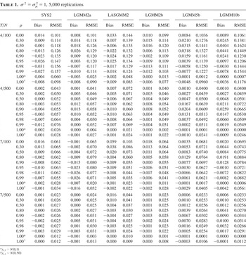
We have generated artificial data from an inclusive model with σ2 = σμ2 = 1 for several values of ρ between 0 and 1 while assuming normality of the data. For the unit root case we have generated two sets of results: for one set the initial observations were drawn from the N(0,1) distribution, and for the other set they were drawn from N(0,50). The first set corresponds to the case b ≈ 0, and the second set corresponds to the case b ≈ ½. The panels have dimensions N = 100 or 500 and T = 4 or 7. The number of replications was 5,000.
The Monte Carlo results are presented in Table 1. We first discuss the results for the two-step estimators and ρ < 1. They indicate that the LGMM2b estimator displays better finite-sample properties than the SYS2 estimator and also performs better than the LGMM2a estimator, especially when N = 100, T = 7, and ρ is close to one. However, when T = 7 and ρ is close to one, the SYS2 estimator outperforms the LGMM2a estimator despite the fact that the latter exploits more moment conditions. The RMSE of the LGMM2b estimator is up to 30% lower than the RMSE of the SYS2 estimator when 0.9 ≤ ρ < 1. Finally, when T = 4 or when T = 7 and N = 500 the RMSE (and in most cases also the bias) of the LASGMM2 estimator is larger than that of the LGMM2b estimator and in many cases, notably when ρ < 0.9, the RMSE of the LASGMM2 estimator is also larger than the RMSE of the SYS2 estimator.
σ2 = σμ2 = 1, 5,000 replications

We now turn to the Monte Carlo results for the unit root case and for the iterative LGMM5b and LGMM10b estimators. Table 1 shows that when ρ = 1 the LGMM2b estimator still has better finite-sample properties than the LGMM2a and SYS2 estimators. Furthermore, the bias and the RMSE of the LGMM estimators are larger when the variance of the initial observations is larger. The latter finding does not hold for the LASGMM2 estimator.
The superefficiency of the iterated LGMM estimator when b ≈ 0 can clearly be seen in the rows corresponding to ρ = 1.00*. When N = 500, all 5,000 LGMM10b estimates lay in fact between 0.9997 and 1.0002. On the other hand when ρ < 1 or when ρ = 1 with b ≈ ½ (ρ = 1.00[dagger]), the RMSEs of the iterated LGMM estimators are higher than the RMSE of the LGMM2b estimator. In particular, when the number of iterations increases, the RMSE of the iterated estimator increases, and so does its mean when T = 4 or when T = 7 and N = 500. As a consequence the bias of the iterated estimator also increases unless ρ is close to one.
Finally the results in Table 1 suggest that the RMSEs of the SYS2 and the LGMM estimators are discontinuous at ρ = 1. These discontinuities are partly related to the fact that some of the elements of E(dm(ρ)/dρ) are discontinuous at ρ = 1 (cf. Lemma 3). As a result, we have, e.g.,

. Moreover, when |ρ| < 1 the optimal LGMM estimators are

-consistent and asymptotically normally distributed, whereas when ρ = 1 they have a nonnormal asymptotic distribution and are in fact superconsistent if b < a.
APPENDIX
Proof of Theorem 1. Both the OLGMM estimator and the optimal Ahn–Schmidt GMM estimator are defined for T ≥ 3. For any value of T ≥ 3, the only difference between these estimators is that the OLGMM estimator exploits the linear moment condition in (15) instead of the nonlinear moment condition in (14). Therefore, to prove that these estimators are asymptotically equivalent, it is sufficient to show for T = 3 that the set of moment conditions exploited by the OLGMM estimator can be obtained by using a one-to-one transformation of the set of moment conditions exploited by the optimal Ahn–Schmidt estimator.
When T = 3, the OLGMM estimator exploits E(m(ρ)) = 0, where mk(ρ), k = 1,2,3,4, are defined in (16). Let us define yi2 = [yi,12 yi,1 yi,2 yi,1 yi,3 yi,22 yi,2 yi,3 yi,32]′. Then there exists a (4 × 6) matrix G such that m(ρ) = Gyi2. Note that G depends on ρ and that rank(G) = 4 unless ρ = 1.
Let S3 be a (3 × 4) selection matrix with [S3]i,i = 1, i = 1,…,3, and zeros elsewhere. The term S3 selects the first three rows of a matrix with four rows. When T = 3, the Ahn–Schmidt estimator exploits E(S3 Gyi2) = 0 and in addition the moment condition in (14), which can be written as E(hyi2) = 0, where h = [ρ3 − ρ2 − ρ + 1 −ρ3 − 2ρ2 + ρ ρ2 + ρ 2ρ2 + ρ − 1 − 2ρ 0]. Thus when T = 3 the Ahn–Schmidt estimator exploits E(Hyi2) = 0, where H′ = [G′S3′ h′].
Let K′ = [S3′ k′], where k = [ρ(ρ − 1) −2(1 + ρ) 0 −1]. It is easily verified that rank(K) = 4, h = kG, and thus E(Hyi2) = KE(Gyi2), which completes the proof. █
Proof of Lemma 2. The result follows immediately from the fact that all these moment conditions in m(ρ) are linear in ρ and E(dm(ρ)/dρ|ρ=1) = [0 −σ2 −σ2 σ2]′. █
Proof of Lemma 3. E(dm(ρ)/dρ|ρ=1) = [0 −σ2 −σ2 σ2]′ whereas under stationarity E(dm(ρ)/dρ) = [1/(1 + ρ)σ2 −1/(1 + ρ)σ2 0 2/(1 + ρ)σ2]′. Hence limρ↑1 E(dm(ρ)/dρ) ≠ E(dm(ρ)/dρ|ρ=1). █
LEMMA 6. Let ρ = 1. Then

Proof of Lemma 6. Trivial.
LEMMA 7. Let ρ = 1. Then

Proof of Lemma 7. When ρ = 1, we have

From this and σ12 = E(yi,12) = σ12N2b + o(N2b) with 0 ≤ b ≤ ½ the lemma follows immediately. █
LEMMA 8. Let ρ = 1. Furthermore, let F1 = diag{1 1 1 Nb−a} and

. Then

, where

and where the values of the elements of

depend on the values of a and b. There are three cases: b = 0, 0 < b < a, and b = a. In all three cases

is positive definite symmetric. When b = a,

is a random matrix, whereas when b < a,

is a constant matrix.
Proof of Lemma 8. Recall that a ≥ ½ and σ12 = σ12N2b + o(N2b) with 0 ≤ b ≤ ½. Thus b ≤ a.
Linearity of the moment conditions implies that

, k = 1,2,3,4. From this we obtain expressions for

, k = 1,2,3,4, when ρ = 1 by substituting the formulas for pk,i(1) and dpk,i(ρ)/dρ, k = 1,2,3,4, which are given in Lemma 6 and (A.1), respectively:

The expressions in (A.2) in turn enable us to establish that

when ρ = 1, where the values of the elements of

depend on the values of a and b:
if b = 0,

if 0 < b < a,

if b = a,

Note that in all three cases the matrix

can be factorized as

where

and where the values of the elements of

depend on the values of a and b. Furthermore, in all three cases

is positive definite symmetric:

Finally note that when b = a,

is a random matrix, whereas when b < a,

is a constant matrix. █
Proof of Theorem 4. Lemma 6 implies that

with

; Lemma 7 implies that

with

if b < ½, and

if b = ½. Moreover,

. Finally, when ρ = 1, Lemma 8 implies that

, where

with F1 = diag{1 1 1 Nb−a}. We can now easily verify the following results:
When b < a:

When b = a = ½:

From the preceding results, the claims in the theorem follow straightforwardly. █
Proof of Corollary 5. When ρ = 1 the asymptotic variance of the iterated OLGMM estimator decreases after each iteration because N1/2+a > Na. Therefore the asymptotic variance of the iterated OLGMM estimator tends to zero when the number of iterations tends to infinity. We need to compare this asymptotic variance with the CR lower bound for ρ = 1. We derive the CR lower bound for ρ = 1 from the likelihood function corresponding to the model yi,t = ρyi,t−1 + εi,t, i = 1,…, N, t = 2,…,T, where yi,1 ∼ i.i.d. N(0,σ12) with σ12 = σ12N2b + o(N2b) and εi,t|yi,1 ∼ i.i.d. N(0,σ2). The CR lower bound can be derived from this likelihood function because the corresponding model is nested within any other panel AR model that reduces to the inclusive panel AR(1) model for ρ = 1. It is easily verified that the CR lower bound for ρ = 1 is given by CR = limN→∞ 2σ2/[(T − 1)((T − 2)σ2 + 2σ12)]. Clearly CR > 0 when b = 0. █
Nonequivalence of the OLGMM Estimator and the Optimal Ahn–Schmidt GMM Estimator for the Inclusive Panel AR(1) Model when ρ = 1.
Let E(m5(ρ)) = 0 denote the nonlinear moment condition in (14) and let p5(ρ) = −(1 + ρ)(p2(ρ) + m5(ρ)). Then it is easily verified that p5(1) = 0, p5(ρ) = −ρ(ρ − 1)σ1 p1(ρ) + (ρ − 1)p2(ρ) + p4(ρ), and

when ρ = 1. The last expression can be used to derive the asymptotic distribution of the elements of the “optimal” weight matrix corresponding to E(p5(ρ)) = 0. Moreover, when ρ = 1,

if b < ½, whereas N−1

if b = ½. Therefore, if in E(p(ρ)) = 0, we replace E(p4(ρ)) = 0 by E(p5(ρ)) = 0, then we will obtain a different optimal weight matrix for E(p(ρ)) = 0, and if b = ½,

will have a different asymptotic distribution. As a result, when ρ = 1, the optimal GMM estimator exploiting E(p(ρ)) = 0 with E(p4(ρ)) = 0 replaced by E(p5(ρ)) = 0 will have a different nonnormal asymptotic distribution than the OLGMM estimator but the same rate of convergence. █