Flight trajectory optimisation for large-scale flights under trajectory-based operations

Z. Yang; Z. Shi; D. Sui; Z. Cui

doi:10.1017/aer.2026.10150

Flight trajectory optimisation for large-scale flights under trajectory-based operations

Published online by Cambridge University Press: 25 March 2026

Z. Shi ,

and

Z. Yang: Affiliation:
China Aeronautical Radio Electronics Research Institute, China
Z. Shi: Affiliation:
China Aeronautical Radio Electronics Research Institute, China Shanghai Jiaotong University: Shanghai Jiao Tong University, China
D. Sui*: Affiliation:
Nanjing University of Aeronautics and Astronautics, China
Z. Cui: Affiliation:
China Aeronautical Radio Electronics Research Institute, China
*: Corresponding author: D. Sui; Email: dong_sui@126.com

Article contents

Abstract
Nomenclature
Abbreviations
Introduction
Problem description
Waypoint capacity evaluation model
Flight trajectory optimisation model
Experiments
Discussion and conclusion
Footnotes
References

Rights & Permissions

Abstract

Effectively improving flight fuel efficiency and optimising operational management while ensuring environmentally sustainable and safe operations is crucial for the global aviation to achieve a successful sustainability transition. Addressing the imperative shift from conventional air traffic flow management (ATFM) to trajectory-based operation (TBO), this paper proposes a large-scale flight trajectory optimisation framework under TBO. The study integrates influencing factors including meteorological conditions, airspace capacity and aircraft performance. With the assistance of an air traffic operation simulation system, flight characteristic information is extracted to construct the optimisation model. The model addresses a multi-objective optimisation problem, balancing sector excess traffic flow against cruise fuel consumption within a priority-based framework, to generate global flight plans with optimal altitude profile and waypoint overflight times. Experiment in Chinese airspace shows the TBO scenario achieves substantial reductions of 66.0% in excess sector traffic and 7.8% in cruise fuel consumption versus baseline scenario. This provides a methodological framework for airspace resource allocation supporting energy conservation and emission reduction.

Keywords

air traffic management trajectory-based operation

Information

Type: Research Article
Information: The Aeronautical Journal , Volume 130 , Issue 1348 , June 2026 , pp. 1978 - 2009

DOI: https://doi.org/10.1017/aer.2026.10150 [Opens in a new window]
Copyright: © The Author(s), 2026. Published by Cambridge University Press on behalf of Royal Aeronautical Society

Nomenclature

$F$: Set of flights, indexed by $f$
$Q$: set of airports, indexed by $q$
$S$: set of sectors, indexed by $s$
$P$: set of waypoints, indexed by $p$
$H$: set of flight levels, indexed by $h$
${H_f}$: adjustable cruise flight level for flight $f$
$h_j^f$: flight altitude when flight $f$ arrives at the j-th waypoint
$M$: set of time periods, indexed by $m$
${W_f}$: set of all operational plans of flight $f$
$ar{r_f}$: destination airport of flight $f$
${T_{slot}}$: minimum adjustable time slot
$t_{i,in}^{f,h}$: time of flight $f$ enters the i-th sector of flight level $h$
$t_{i,out}^{f,h}$: time of flight $f$ exits the i-th sector of flight level $h$
$t_j^f$: time of flight $f$ flying over the j-th waypoints
$t_{arr}^f$: time of arrival at the destination airport of flight $f$
$s_h^f$: list of sectors passed by flight $f$ at flight level h
$s_i^{f,h}$: I-th sectors passed by flight $f$ at flight level h
${p^f}$: list of waypoints passed by flight $f$
$p_j^f$: J-th waypoint passed by flight $f$
$d_a^b$: flight segment distance between waypoint a and waypoint b
$VW_a^b$: average wind speed between waypoint a and waypoint b
$O_s^m$: excess traffic flow in sector s during time period m
$C_s^m$: capacity of sector s during time period m
$C_q^m$: capacity of airport q during time period m
$C_p^{m,h}$: capacity of waypoint p at flight level h during time period m
${C_P}$: capacity of waypoint p
$u_e^{f,h}$: E-th waypoint timing adjustment scheme set of flight $f$ at flight level h
$\chi $: waypoint timing factor
$\eta $: aircraft type distribution function
$\psi $: headway distribution function
$\lambda $: traffic flow distribution function
$\Omega $: acceptable fluctuation threshold
$\delta $: heading angle
$HD$: altitude profile similarity
$\ell $: silhouette coefficient

Abbreviations

ATFM: air traffic flow management
TBO: trajectory-based operations
ATOSS: air traffic operations simulation system
BADA: base of aircraft data
SESAR: single European sky ATM research
NextGen: United States’ next generation air transportation system
CAAMS: China’s civil aviation ATM modernisation strategy
ANSP: air navigation service providers
PBN: performance-based navigation
DBSCAN: density-based spatial clustering of applications with noise
ECMWF: European Centre for Medium-Range Weather Forecasts

1.0 Introduction

With global demand for air transport continuing to grow, enhancing flight fuel efficiency and reducing the environmental impact of aviation, while maintaining safe and efficient air traffic operations, has emerged as a central goal and critical challenge for transforming and developing the global air transport system. Major initiatives – including Europe’s Single European Sky ATM Research (SESAR) program, the United States’ Next Generation Air Transportation System (NextGen), and China’s Civil Aviation ATM Modernisation Strategy (CAAMS) – have redefined the vision for future air traffic operations by incorporating new environmental and sustainable development objectives [Reference Kistan, Gardi and Sabatini1–Reference Prandini, Putta and Hu3]. These initiatives collectively establish TBO as the future operational paradigm for global air traffic management systems. TBO facilitates the strategic planning, management and optimisation of the entire flight process through precise temporal control, efficient air-ground information exchange and aircraft capabilities for high-precision spatiotemporal trajectory execution [Reference Liang, Sandhu and Kasper4, Reference Toratani5]. This approach thereby effectively addresses both the diverse needs of users and the complexity of traffic flow. Therefore, research on flight trajectory optimisation within the TBO framework has emerged as a critical frontier topic in air traffic management.

The optimisation objectives and methods for flight trajectory planning vary depending on the specific flight phase during operations. For the climb and descent phases, optimisation primarily targets the vertical trajectory profile, specifically continuous climb operations (CCO) [Reference Prats, Puig and Quevedo6–Reference Ho-Huu, Hartjes and Visser8] and continuous descent operations (CDO) [Reference Solak and Chen9, Reference Soler, Zou and Hansen10]. CCO and CDO can effectively reduce fuel consumption, noise and pollutant emissions, and are important technologies for improving flight operational efficiency and economic benefits during takeoff and landing phases. For the cruise phase, trajectory optimisation primarily focuses on flight distance, fuel consumption and time cost, while meeting required time of arrival (RTA) constraints [Reference Dancila and Botez11–Reference Murrieta-Mendoza, Beuze and Ternisien13]. Lovegren et al. [Reference Lovegren and Hansman14] improved fuel efficiency through optimisation of altitude and speed profiles. Williams et al. [Reference Williams, Noland and Toumi15] investigated the impact of flight altitude on wake vortex generation and engine emissions, proposing that strategic flight-level assignment can reduce carbon dioxide (CO₂) emissions and contrail formation. Gardi et al. [Reference Gardi, de Ridder and Sabatini16] integrated aircraft trajectory planning with air traffic management systems, developing a framework for collaborative four-dimensional trajectory (4DT) planning.

However, existing studies rarely systematically incorporate critical factors like sector capacity-flow balance and airspace resource constraints prevalent in actual operations. The growing prominence of airspace resource saturation necessitates precise, dynamic and collaborative airspace resource management. In this context, TBO integrates time-based management (TBM) and performance-based navigation (PBN) technologies to generate four-dimensional trajectories, thereby planning collaborative optimisation schemes that satisfy the requirements of both airspace users and air navigation service providers (ANSPs) [Reference Chen, Hu and Yang17]. Within the framework of TBO research and implementation, two complementary yet distinct levels are often recognised: network-TBO and air traffic control (ATC)-TBO [Reference Caranti, Ribeiro and Carré18, Reference Sui and Zhang19]. Network-TBO focuses on strategic/pre-tactical air traffic flow management for large-scale networks, aiming to balance traffic, alleviate congestion and enhance airspace capacity/efficiency. Decisions typically involve optimising cruise altitudes, waypoint transit times and macroscopic route planning for spatiotemporal coordination. ATC-TBO emphasises tactical execution within sectors, centred on real-time collaboration between controllers and flight crews using 4D trajectories. Its focus includes ensuring conformance, resolving short-term conflicts, responding to sudden weather changes and maintaining separation via tactical instructions such as speed adjustments, direct routings or flight-level changes.

Relevant scholars have already conducted related research on the optimisation of multiple flight trajectories. Chaimatanan et al. [Reference Chaimatanan, Delahaye and Mongeau20] combined network theory with trajectory planning to construct an optimisation model for waypoint allocation and controlled time of arrival (CTA) design during the cruise phase of intercontinental flights. This method offers significant advantages for long-range flight trajectory planning. Zhou et al. [Reference Zhou, Zhang and Wang21] established a multi-objective collaborative trajectory planning model considering airspace congestion, potential conflicts and fuel consumption, and solved the model using non-dominated sorting genetic algorithm (NSGA)-III. Optimisation results indicate the model effectively reduces fuel consumption while significantly alleviating airspace congestion and mitigating conflicts. Liu et al. [Reference Liu, Li and Xie22] focused on city-pair flights under capacity constraints, improving fuel efficiency through collaborative optimisation of flight paths, vertical profiles and speeds, and analysed the spatiotemporal evolution of congestion location and severity under the optimal solution.

Research methodologies for such studies can be broadly classified into three categories: mathematical programming methods, simulation-based optimisation methods and machine learning methods. Mathematical programming methods facilitate the flexible definition of optimisation objectives and enable the imposition of precise constraints on trajectory optimisation problems (e.g. operational constraints, speed limits and altitude adjustments). They can also incorporate system randomness and enhance solution robustness. Common methods include dynamic programming (DP) [Reference Ahmed, Bousson and Coelho23], nonlinear programming (NLP) [Reference Lim, Gardi and Sabatini24, Reference Tian, He and Xu25] and heuristic algorithms [Reference Hartjes and Visser26–Reference McEnteggart and Whidborne28]. Although mathematical programming methods offer flexible modeling capabilities, their applicability is challenged by the high complexity of actual flight operational details and dynamic constraints. This often necessitates simplifying certain factors or introducing assumptions that do not fully reflect real-world operational conditions, potentially compromising model realism and accuracy.

Simulation-based optimisation methods are primarily employed to study issues such as aircraft CO₂ emissions, the climate impact of contrails [Reference Gao29, Reference Sridhar, Ng and Chen30] and the trade-offs between climate impact and operational costs [Reference Chen, Sridhar and Ng31, Reference Xue, Ng and Hsu32]. Their key modeling advantage is the ability to incorporate complex flight operation details that are difficult to represent using mathematical programming methods. This enables the construction of simulation scenarios that more closely resemble actual air traffic network environments, thereby enhancing model accuracy and realism. However, a major limitation of this approach is optimisation efficiency; computational costs often increase exponentially with the number of variables, resulting in inefficient simulation execution.

Recently, machine learning methods have found widespread application in air traffic management, including fuel consumption estimation [Reference Baumann and Klingauf33, Reference Wahid, Bukhari and Maqsood34], traffic flow prediction [Reference Zang, Zhu and Gao35, Reference Lyu, Zhang and Wan36] and flight trajectory prediction [Reference Wu, Yang and Chen37–Reference Ma and Tian39]. These data-driven methods identify complex patterns within historical air traffic data, enabling efficient and accurate prediction and regression analysis of key operational features like traffic flow and flight trajectories. Currently, machine learning applications in air traffic management are predominantly focused on predictive assistance tasks, and their scope remains somewhat limited.

Table 1.

Literature on flight trajectory optimisation

A table comparing various authors' research on flight trajectory optimization, focusing on objectives, scope, weather conditions, finite airspace resources, waypoint capacity, global optimality, and integration with TBO.

Table 1 Long description

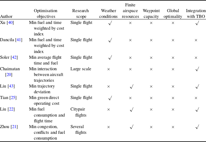
The table presents a comparison of research on flight trajectory optimization by different authors. It includes columns for optimization objectives, research scope, weather conditions, finite airspace resources, waypoint capacity, global optimality, and integration with TBO. The table has eight rows, each representing a different author's work. Key authors and their objectives include Xu, who aims to minimize fuel and time weighted by cost index for single flights, Dancila with similar objectives, Soler focusing on minimizing average flight time and fuel, Chaimatan addressing interaction between aircraft trajectories on a large scale, Liu minimizing trajectory deviation for single flights, Tian aiming to minimize green direct operating cost, another Liu working on minimizing fuel consumption and flight time for citypair flights, and Zhou focusing on minimizing congestion, conflicts, and fuel consumption for several flights. Notable trends include the emphasis on single-flight optimization and the consideration of weather conditions and finite airspace resources.

Table 1 lists some scholars’ research on flight trajectory optimisation problems and compares them in terms of optimisation objectives, research scope, weather conditions, finite airspace resources, waypoint capacity, global optimality and integration with TBO. Comparative analysis reveals that despite extensive research on flight trajectory optimisation, significant research gaps persist in three key areas:

• Limited scope and targets: Existing studies predominantly focus on optimising individual flights or specific city-pair groups, neglecting large-scale or regional flight trajectory optimisation.
• Inadequate incorporation of key operational factors: critical in-flight factors, such as the spatiotemporal coupling of airspace capacity and traffic flow, as well as regional meteorological variations, receive insufficient attention. Notably, temperature and crosswinds can significantly influence flight trajectory optimisation outcomes.
• Under-addressed waypoint capacity constraints: waypoint capacity constitutes a critical bottleneck in airspace resource management. However, existing flight trajectory optimisation studies predominantly address sector capacity constraints, offering limited detailed assessment and modeling of throughput capacity at congested waypoints.

Given airspace requirements and considering the spatial connectivity and operational interdependence of resources within the air traffic network, airspace congestion can be alleviated by optimising the temporal and spatial distribution of air traffic flow. This is achieved through precise control of aircraft arrival times at each waypoint along their flight trajectories. This control not only facilitates interval allocation and flight sequencing based on spatiotemporal data but also enables predicting traffic conditions within congested airspace regions. This significantly enhances both air traffic predictability and route network operational efficiency.

Building upon these principles, the problem of optimising flight trajectories for numerous flights is addressed. The core methodology involves mapping the operational state of airspace into a spatio-temporal flow distribution matrix for regional control sectors across discrete time periods. Through autonomous adjustment of cruise altitudes and speeds, integrated planning for large-scale flight management is conducted under a priority-based optimisation strategy to concurrently mitigate sector excess traffic flow and reduce fuel consumption. The primary contributions of this study are summarised as follows:

• A general method for evaluating waypoint capacity under TBO is proposed. This method incorporates four key operational parameters extracted from historical data (aircraft type distribution, headway distribution, waypoint network structure and traffic flow distribution) to assess waypoint capacity. By leveraging Monte Carlo simulation, it provides a scientific basis for evaluating the rationality of airspace traffic distribution.
• A simulation-assisted optimisation framework for large-scale flight trajectory optimisation is developed. To address the high-dimensional nonlinearity inherent in such problems, this framework integrates mathematical programming with simulation. It pre-extracts operational features from an air traffic simulation system, transforming the original nonlinear formulation into a linear one, thereby substantially improving computational efficiency and scalability.
• Large-scale flight trajectory optimisation experiments are conducted using real-world operational data. Based on actual flight schedules, China’s air traffic network and 24-hour meteorological scenarios, the experimental results demonstrate that the proposed TBO-based approach reduces excess sector traffic flow by 66.0% and cruise-phase fuel consumption by 7.8% compared to the baseline scenario. These findings underscore the dual benefits of optimising altitude profiles and waypoint overflight times: effectively mitigating airspace congestion while enhancing fuel efficiency.

The remainder of this paper is organised as follows. Section 2 presents the problem description. Section 3 details the Monte Carlo simulation-based waypoint capacity evaluation model. Section 4 introduces the TBO operation scheme generation method, and the large-scale flight trajectory optimisation model, including its objective function, decision variables and constraints. Section 5 describes the experimental data and environment and presents the results of large-scale flight trajectory optimisation experiments using China’s full-day flight operations. Results are analysed regarding sector congestion mitigation and fuel consumption reduction, validating the optimisation model’s accuracy. Section 6 concludes the paper and outlines future research directions.

2.0 Problem description

In the conventional air traffic management system, flow management primarily relies on ground holding strategies, which adjust flight departure times. While this approach offers enhanced safety and lower implementation costs, the pre-determined departure times, coupled with the inherent uncertainties of air traffic operations (e.g. weather changes and temporary airspace restrictions), can cause deviations in the scheduled slot times for flights entering sectors, potentially leading to sector congestion.

The essence of the above method is to convert airborne delays into ground delays; without sophisticated management tools, it is impossible to achieve true airspace resource balancing. TBO, on the other hand, aims to safely and precisely control aircraft operations by dynamically updating and optimising flight trajectories based on airspace resource availability and real-time flight status, to enable dynamic management of four-dimensional trajectories throughout the entire flight through collaborative decision-making. Therefore, within a large airspace, flight trajectory optimisation based on the TBO model is the future direction of refined air traffic management operations.

Figure 1.

Framework concept for large-scale flight trajectory optimisation.

Illustration of flight trajectory optimization framework with flight paths, sectors, and influencing factors.

Figure 1 Long description

The image illustrates a framework concept for optimizing large-scale flight trajectories. It features a map with flight paths, sectors, and waypoints, highlighting the extraction of flight operation features. The diagram includes various sectors and waypoints, with flight paths marked in different colors. It also shows the adjustment of cruising altitudes and waypoint overflight times. Additionally, the image depicts factors influencing airspace operation, such as wind patterns, temperature variations, airport capacity, and airspace capacity. The overall concept emphasizes the optimization of flight trajectories under the Trajectory-Based Operation (TBO) model.

This paper addresses the following problem: given a static air traffic network and its associated airspace configuration (comprising airports ( ${\rm{Q}}$ ), sectors ( ${\rm{S}}$ ), predefined routes between city pairs (L), waypoints ( ${\rm{P}}$ ), among others), along with the initial flight plans of the target flights. We aim to develop a method that, while respecting aircraft performance constraints, allows flights to autonomously update and select optimal cruise altitude profiles and waypoint overflight times after departure based on real-time traffic distribution and meteorological conditions. By strategically controlling waypoint passage times, this approach enhances air traffic predictability and network operational efficiency, as illustrated in Fig. 1. The proposed methodology falls within the network-level TBO domain, focusing on system-wide optimisation of traffic distribution and fuel efficiency at the pre-tactical stage from a global flow management perspective. This strengthens network-level flow management and lays the foundation for higher-level trajectory synchronisation.

To address large-scale flight trajectory optimisation, this work integrates mathematical programming with high-fidelity simulation. Using an air traffic simulation system, we establish a mapping between planned and simulated trajectories by extracting key operational metrics (e.g. sector entry/exit times and waypoint overflight times) to generate baseline operational profiles. Under constraints from weather, air traffic control regulations and aircraft performance, we jointly optimise speed and altitude profiles to produce feasible 4D trajectories compliant with TBO. This reformulates the original nonlinear problem into an integer linear programming (ILP) model, which is solved exactly using commercial solvers, significantly reducing computational complexity and solution time.

3.0 Waypoint capacity evaluation model

Prior to large-scale flight trajectory optimisation, airspace capacity evaluation must be performed. This evaluation is strongly influenced by the target airspace’s geographic configuration and traffic flow patterns. Conventional approaches typically use sectors as fundamental operational units, evaluating traffic distribution feasibility against sector capacity thresholds. However, in the TBO scenario, the bottleneck in traffic flow essentially lies in the traffic capacity constraints at waypoints. To address this, we develop a Monte Carlo simulation-based method for evaluating waypoint capacity.

3.1 Flight trajectory feature extraction

Due to various factors, such as weather, air traffic flow control and military activities, an aircraft’s altitude, speed and position may deviate from its pre-planned flight path and altitude profile. However, due to the similarity between daily flight schedules, flights operating on the same flight path exhibit a certain degree of operational inertia in their flight trajectory. Accordingly, we process historical trajectory data to distill key recurrent patterns, both horizontal flight paths and vertical flight profiles, forming a flight trajectory characteristics database (Fig. 2).

Figure 2.

Extracting flight trajectory information process.

Figure 2 Long description

The image contains four main sections. The first section, titled 'City pairs Flight trajectory,' shows a line graph depicting flight altitude against flight distance for various city pairs. The second section, 'Flight profile Clustering,' presents four line graphs, each representing different clusters of flight profiles based on flight distance and altitude. The third section, 'Flight characteristics database,' illustrates a diagram of a flight path from departure to destination airport, including details such as city pairs, flights, cruising altitude, and flight path. The fourth section, 'Flight feature extraction,' shows a diagram of flight trajectories with waypoints, pre-trajectory, and actual trajectory. The process involves clustering flight profiles, extracting flight features, and collecting flight characteristics to build a database. All values are approximated.

The first step is to identify the waypoints for extracting trajectory information. Matching rule specification: create a 15 km-radius buffer zone centred on the target waypoint; when consecutive trajectory points fall within the buffer zone, confirm the aircraft has passed the waypoint; select the trajectory point with the minimum distance to the waypoint as the feature extraction point. For each successfully matched waypoint, the following operational parameters are extracted: aircraft altitude, speed and overpass time information. Then integrates with flight plan datasets to generate trajectory features for flights operating on the same city pair. Obtain the flight altitude profiles of flights for each city, providing data support for the subsequent extraction of the flight profiles of the flights.

Even for flights with identical origin–destination airports and planned routes, their actual operational altitude profiles exhibit variability, yet these variations demonstrate identifiable regularity patterns. To extract representative altitude profile patterns for city-pair flights, this study applies the clustering algorithm to analyse altitude profile samples. Through outlier removal, statistically significant cluster categories are identified, with each cluster centroid serving as the nominal flight altitude profile for its respective city pair. Unlike traditional clustering algorithms, density-based spatial clustering of applications with noise (DBSCAN) does not require pre-defining the number of clusters, instead forming clusters based solely on data point density [Reference Hanafi and Saadatfar44]. This algorithm requires two parameters: ε, the maximum neighbourhood radius, and minPts, the minimum number of points required to form a dense region. We extract features from flight trajectory information, including cruise altitude, mean altitude and altitude standard deviation, to compute pairwise profile similarity. The altitude profile similarity $H{D_{i,j}}$ between the i-th and j-th profiles is calculated using Equation (1), where h ₁, _i , h _2, _i and h _3, _i denote the cruise, mean and standard deviation of altitude for i-th profile. Two altitude profiles are considered similar if their distance $H{D_{i,j}}$ is less than ε. If a profile has at least minPts similar profiles within its ε-neighbourhood, they are grouped into a cluster.

(1)

\begin{align} H{D_{i,j}} = \sqrt {{{\left( {{h_{1,i}} - {h_{1,j}}} \right)}^2} + {{\left( {{h_{2,i}} - {h_{2,j}}} \right)}^2} + {{\left( {{h_{3,i}} - {h_{3,j}}} \right)}^2}} \end{align}

The silhouette coefficient $\ell $ quantifies how similar a sample is to its own cluster compared to the nearest other cluster. The coefficient for a single sample is defined by Equation (2). We perform clustering on flight altitude profiles by testing various (ε, minPts) parameter combinations. The optimal clustering result is selected by comparing the average silhouette coefficients across different parameter sets. As DBSCAN does not explicitly compute cluster centroids, for each cluster we calculate the average distance from every profile to all others within the same cluster. The profile exhibiting the smallest average intra-cluster distance (i.e. the most central profile) is then chosen as the cluster representative, or nominal altitude profile. This nominal profile serves as a reference for calibrating cruise altitudes on inter-city flight trajectories.

(2)

\begin{align} \ell = \frac{1}{n}\sum\limits_{z = 1}^n {\frac{{\sigma \left( z \right) - \mu \left( z \right)}}{{\max \left( {\mu \left( z \right),\sigma \left( z \right)} \right)}}} \end{align}

In Equation (2), $\mu \left( z \right)$ denotes the average distance between the z-th profile and all other profiles in the same cluster, measuring intra-cluster compactness. $\sigma \left( z \right)$ is the average distance from the z-th profile to the profiles in the nearest neighbouring cluster, measuring inter-cluster separation. The overall silhouette score $\ell $ is the mean of all individual values and serves as a metric for evaluating global clustering quality.

3.2 Concept of waypoint capacity

Waypoint capacity is defined as the maximum aircraft throughput per unit time under given airway network topology, control rules and safety requirements [Reference Zhang, Shan and Zhang45]. Based on connectivity, waypoints are classified as intersections or non-intersections, where the connectivity degree denotes the number of segments meeting at an intersection. The traffic flow distribution $\lambda $ quantifies flow imbalance at a waypoint. Route segments at given altitudes may be categorised as trunk (high-traffic) or feeder (low-traffic) routes based on traffic volume, with distribution varying across altitudes due to operational constraints, as shown in Fig. 3.

Figure 3.

Aircraft operation scene at waypoints.

Figure 3 Long description

The image illustrates an aircraft operation scene at waypoints, showing different flight levels and routes. It features three main flight levels: idle, near-saturation, and congested. Each level is represented by different colors: light blue for idle, yellow for near-saturation, and pink for congested. Aircraft are shown following trunk routes and feeder routes, indicated by purple and green lines respectively. Waypoints are marked with red triangles. The image also shows a transition from multiple flight levels converging at a waypoint to a single congested flight level. Arrows indicate the direction of flight paths, and the image highlights the interaction between different flight levels and routes at waypoints.

Flight levels are categorised as:

• Idle flight level: Traffic flow significantly below capacity, causing resource inefficiency.
• Near-saturation flight level: Traffic flow approaching capacity, increasing conflict risk.
• Congested flight level: Traffic flow exceeding capacity, causing efficiency degradation.

Figure 4.

Statistical results of waypoint operational characteristics. (a) Aircraft type distribution (b) Headway distribution.

A bar graph showing aircraft type distribution and headway distribution.

Figure 4 Long description

The bar graph consists of two parts: (a) Aircraft type distribution and (b) Headway distribution. In part (a), the x-axis represents different flight models, including B 738, A 320, A 321, A 319, A 333, B 737, B 388 M, A 332, E 190, B 789, B 777 W, B 752, B 739, B 778, and A 20 N. The y-axis shows the probability of each aircraft type. The B 738 has the highest probability, followed by the A 320 and A 321. In part (b), the x-axis represents the release interval in seconds, ranging from 180 to 840 seconds. The y-axis shows the frequency of time intervals. The frequency peaks around 240 seconds and gradually decreases as the release interval increases. The blue bars represent the frequency of time intervals, and the red line represents the fitting curve. All values are approximated.

To enhance simulation fidelity with actual operations and controller separation management, we employ Monte Carlo simulation to evaluate waypoint operational dynamics. It is ideal for stochastic systems like air traffic, where operations are influenced by numerous random factors including clearance strategies, aircraft performance variations and dynamic traffic patterns [Reference Andreeva-Mori46, Reference Churchill and Lovell47]. We construct a multivariate probability model to govern these uncertainties within the simulation. Key parameters for waypoint capacity assessment include:

• Aircraft type distribution: Affects performance characteristics (speed, altitude), indirectly impacting the capacity of waypoints. Figure 4(a) ranks aircraft type proportions and fits the probability selection function $\eta $ .
• Headway distribution: Controller separation decisions directly affect capacity. Peak-period headway data from busy waypoints were analysed for each flight level. Recorded transit times during peak hours yielded headway distributions $\psi $ , with fitted functions (Fig. 4(b)) setting initial simulation times.
• Network topology: The air route network’s topology provides the structural foundation for flight path generation. Key waypoints, serving as convergence/divergence nodes, govern network efficiency through their throughput capacity; their configuration determines airspace capacity distribution and bottleneck locations.
• Traffic flow distribution: During the evaluation process, based on actual operating data, the traffic flow distribution $\lambda $ for different flight paths at each altitude level should be statistically calculated and compiled as the basis for generating flight paths in simulation experiments. Figure 5 illustrates this for the HFE waypoint.

Figure 5.

Network topology and traffic flow distribution at waypoint HFE. (a) 7200 m, (b) 8400 m, (c) 9200 m, and (d) 9500 m.

A line graph showing network topology and traffic flow distribution at waypoint HFE at different altitudes: 7200 meters, 8400 meters, 9200 meters, and 9500 meters.

Figure 5 Long description

The line graph displays network topology and traffic flow distribution at waypoint HFE across four different altitudes: 7200 meters, 8400 meters, 9200 meters, and 9500 meters. Each subplot represents a specific altitude, with the x-axis indicating longitude and the y-axis indicating latitude. The graph includes multiple colored lines representing different flight paths and their respective trajectories. The red star labeled HFE marks a specific point of interest in each subplot. The trajectories vary in direction and spread, illustrating the changes in network topology and traffic flow distribution as altitude increases. All values are approximated.

3.3 Monte Carlo simulation method

3.3.1 Assumption

Before setting up the simulation scenario, it is necessary to first explain the prerequisites for the waypoint capacity assessment method. The specific assumptions are as follows:

• Determine maximum throughput capacity at waypoints under saturated demand.
• When the altitude layer is determined, the set of initial flight paths available for selection in the experimental scenario is known.
• Without considering changes in the speed of aircraft passing through waypoints, the motion trajectory along the route is approximated as linear motion.

3.3.2 Scene construction

Taking the waypoints awaiting evaluation of traffic flow capacity as the core, an airspace simulation scenario is constructed by integrating the connected waypoints and the segments forming the edges. In this experimental scenario, all aircraft strictly adhere to the height layer allocation principle: when an aircraft flies at an odd altitude layer, its true heading angle (relative to true north) must be within $(0,{\rm{ }}180^\circ ]$ , with the flight direction from west to east; when an aircraft flies at an even altitude layer, its true heading angle (relative to true north) must be within $(180,{\rm{ }}360^\circ ]$ , with the flight direction from east to west. A flight path is defined as the complete link from aircraft input point – aircraft input segment – evaluation waypoint – aircraft output segment – aircraft output point. Assuming that there are n selectable flight paths at a certain altitude layer in the simulation scenario, the set of flight paths is $L = \{ {L_1},{L_2}, \ldots \ldots ,{L_n}\} $ , and the corresponding path flow ratio set is $\lambda = \{ {\lambda _1},{\lambda _2}, \ldots \ldots ,{\lambda _n}\} $ . The path selection probability is based on the flow ratio.

To ensure flight safety, aircraft separation control standards are strictly enforced during the simulation process. Aircraft at the same altitude level must maintain a horizontal safety separation $L$ when passing through waypoints. For any two aircraft ${f_1}$ and ${f_2}$ at the same flight level and at the same time, the minimum safety separation $L$ is determined based on the heading angles $\delta $ of the two aircraft and their respective motion states at that moment. Table 2 defines the minimum safety separation $L$ corresponding to two motion states: same direction and crossing ( ${\delta _0}$ is critical angle of motion state). 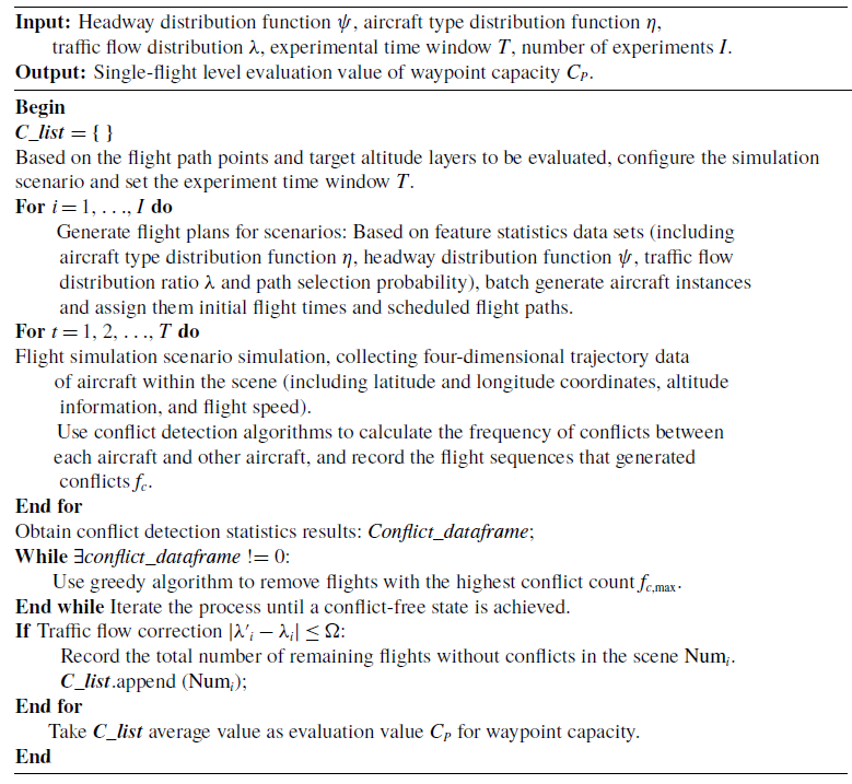When the horizontal distance between two aircraft is less than minimum safety separation $L$ at the same time, a conflict is deemed to occur. For aircraft involved in conflicts, the total number of conflicts with other aircraft in the scene is counted, yielding the conflict detection statistical result. The aircraft with the highest number of conflicts in the scene is prioritised for removal until no conflicts remain in the scene, the pseudocode is shown in Algorithm 1.

Table 2.

Minimum safety separation settings

Table 2 Long description

A table with two rows and three columns outlines the minimum safety separation settings for aircraft. The columns are labeled Judgement criteria, Motion state, and L (km). The first row indicates that when the absolute difference in heading angles is less than a critical angle, the motion state is same direction, requiring a separation of fifteen kilometers. The second row shows that when the absolute difference in heading angles is between the critical angle and one hundred eighty degrees, the motion state is crossing, requiring a separation of twenty-five kilometers.

To ensure that there are no conflicts in the simulation scenario, this study achieves a conflict-free state by iteratively removing conflicting aircraft during the conflict resolution process. However, this process may cause distortion in the traffic flow distribution. To control the degree of distortion, a traffic flow proportion deviation constraint mechanism is established: the initial flight path traffic flow proportion is ${\lambda _i}$ , and the corresponding route traffic flow proportion after removing the conflicting aircraft is ${\lambda '_i}$ . An acceptable fluctuation threshold $\Omega $ is set to maintain the structural stability of the traffic flow distribution, as shown in Formula (3).

(3)

\begin{align} \left| {{{\lambda '}_i} - {\lambda _i}} \right| \le \Omega ,\forall {\lambda _i} \in \lambda \end{align}

Algorithm 1:

Monte Carlo Simulation Method for Waypoint capacity evaluation

An equation representing the minimum safety separation L for aircraft at the same flight level based on heading angles delta and motion states.

Algorithm 1: Long description

The equation shows the minimum safety separation L for aircraft at the same flight level, which is determined by the heading angles delta of the two aircraft and their respective motion states. The separation is defined as 15 kilometers for aircraft moving in the same direction when the absolute difference between their heading angles is less than a critical angle delta zero. For aircraft in a crossing motion state, the separation increases to 25 kilometers when the absolute difference between their heading angles is between the critical angle delta zero and 180 degrees. This separation ensures flight safety by preventing conflicts when the horizontal distance between two aircraft is less than the minimum safety separation L.

4.0 Flight trajectory optimisation model

4.1 Fuel consumption model

Aircraft flight simulation is performed using dynamic models based on the base of aircraft data (BADA)’s point mass model (PMM) and total-energy model (TEM). The TEM, as shown in Equation (4), states that the rate of work done by forces acting on the aircraft per unit time equals the combined growth rate of potential and kinetic energy, that is:

(4)

\begin{align} Mg\frac{{{\rm{d}}H}}{{{\rm{d}}t}} + MV\frac{{{\rm{d}}V}}{{{\rm{d}}t}} = (Thr - D) \cdot V \end{align}

In Equation (4), M is the aircraft mass [kg]. V is the true airspeed [m/s]. Thr is the thrust acting parallel to the aircraft velocity vector[N]. D is the aerodynamic drag[N]. $d/dt$ is the time derivative. L denotes lift, which along with drag are typically expressed as:

(5)

\begin{align} L &= \frac{1}{2}\rho {V^2} \cdot {C_L} \cdot S \\[-10pt] \nonumber\end{align}

(6)

\begin{align} D &= \frac{1}{2}\rho {V^2} \cdot {C_D} \cdot S \\[6pt] \nonumber \end{align}

In Equations (5) and (6), $\rho $ is the air density [kg/m³]. $V$ is the true airspeed [m/s]. $S$ is the wing reference area [m²]. ${C_L}$ and ${C_D}$ denote the lift coefficient and drag coefficient, respectively. Under standard conditions, the drag coefficient, ${C_D}$ is specified as a function of the lift coefficient ${C_L}$ .

(7)

\begin{align} {C_L} &= \frac{{2Mg}}{{\rho {V^2}S\cos \varphi }}\\[-6pt] \nonumber \end{align}

(8)

\begin{align} {C_D} &= {C_{D0}} + {C_{D2}}C_L^2 \\[10pt] \nonumber \end{align}

In Equations (7) and (8), $\varphi $ is the bank angle, ${C_{D0}}$ is the parasitic drag coefficient, ${C_{D2}}$ is the induced drag coefficient. For jet-powered aircraft, the cruise-phase fuel flow rate can be determined using Equation (9), while the fuel consumption is calculated via Equation (10).

(9)

\begin{align} ff = {C_{f{\rm{cr}}}} \cdot {C_{f1}} &\times \left(1 + \frac{V}{{{C_{f2}}}}\right) \times Thr\ {\rm{Cruise}} \\[-10pt] \nonumber \end{align}

(10)

\begin{align} {\rm{FF}} &= \int {ff{\rm{ }}dt} \\[9pt] \nonumber \end{align}

In the above equations, ${C_{f1}}$ , ${C_{f2}}$ , and ${C_{f{\rm{cr}}}}$ are the fuel computation parameters provided by BADA3.11 [Reference Sun, Hoekstra and Ellerbroek48], with ${\rm{FF}}$ and respectively denoting fuel mass [kg]. The International Civil Aviation Organisation (ICAO) engine emissions databank (EDB) is employed to calculate pollutant emissions, as formulated in Equation (11).

(11)

\begin{align} E = EI \cdot FF \end{align}

$E$ denotes the mass of pollutant emissions [g], $FF$ represents fuel burn [kg] and $EI$ is the emission index [g/kg]. The emission index is engine-type dependent, with distinct values for different pollutants across flight phases and engine models.

4.2 TBO flight operation plan

To overcome the technical bottleneck of parameter acquisition for large-scale flights, this paper proposes a simulation-assisted parameter extraction framework. Specifically, each flight plan is simulated via an air traffic operation simulation system to generate trajectory data and extract key model parameters – including sector entry/exit times and waypoint overflight times (Fig. 6). This pre-simulation step reduces the computational burden of the actual optimisation and transforms the original nonlinear problem into a linear formulation. An ILP model is then established to precisely identify the optimal flight operation plan.

Figure 6.

Simulation extraction of flight operation characteristics.

A diagram illustrating flight operation characteristics with sectors, waypoints, and time periods.

Figure 6 Long description

The diagram depicts a flight path from a departure airport to a destination airport, passing through multiple sectors and waypoints. The flight path is divided into segments, each with specific entry and exit times for different sectors and waypoints. The diagram includes labels for departure time, waypoint passing times, waypoint crossing altitudes, sector entry and exit times, and landing time. The flight path is shown as a series of connected points, each representing a waypoint with associated times and altitudes. The sectors are color-coded and labeled, indicating different regions of airspace. The diagram also includes tables listing waypoint names, waypoint passing times, waypoint crossing altitudes, sector names, sector entry times, and sector exit times.

Rational adjustments to flight altitude profiles and speeds can effectively mitigate traffic congestion and enhance fuel efficiency. Leveraging the simulated flight operation characteristics as an initial scenario, this section generates a set of feasible trajectories for each flight under TBO, based on actual constraints, including aircraft performance, meteorological conditions and airspace restrictions, as shown in Fig. 7. After obtaining the set of optional cruise altitude profiles ${{\rm{H}}_{{f}}}$ for the flight to be optimised based on historical data (see Section 3.1 for details), this set serves as the adjustable optimisation range for the flight’s cruise altitude. For flight $f$ , under a set cruise altitude $h$ , the entry sector time and exit sector time of the sector ${s_i}$ are ${t_{i,in}}$ and ${t_{i,out}}$ , respectively. The starting waypoint and ending waypoint of the cruise phase are ${p_a}$ and ${p_b}$ , respectively, for any time-adjusted waypoint ${p_e}$ , $a \lt e \lt b$ , the time-adjustable set ${u_e}$ of waypoints ${p_e}$ is first determined based on flight performance and meteorological factors, with the criteria for time adjustment as shown in Equations (12) and (13).

(12)

\begin{align} \chi = \left\{ {\begin{array}{l@{\quad}c}1 {}& {if{\rm{ }}{t_e} - {t_a} + n{T_{{\rm{slot}}}} \in \Omega }\\[2pt]0 & {}{else}\end{array}} \right.,n = \pm 1, \pm 2, \ldots ..,a \lt e \le b \end{align}

(13)

\begin{align} \vartheta = \left[ {\frac{{d_{{p_a}}^{{p_e}}}}{{V_{\max }^h + VW_a^e}},\frac{{d_{{p_a}}^{{p_e}}}}{{V_{\min }^h + VW_a^e}}} \right]\end{align}

Figure 7.

TBO flight operation adjustment plan.

Figure 7 Long description

The image contains multiple graphs and charts illustrating a TBO flight operation adjustment plan. On the left side, there are three distinct sections: Flight plan, Speed limit, and Wind. The Flight plan section shows a graphical representation of a flight path with altitude and distance markers. The Speed limit section features a graph depicting cruising speed ranges and boundaries over different flight distances. The Wind section includes a wind speed and direction map. On the right side, there are two columns labeled Original plan and Adjustable plan, each containing three horizontal timelines with aircraft icons and colored segments representing different flight phases. The timelines are divided into sectors with time slots marked. The Flying through sector time is shown in light brown, and the Waypoint overflight time is marked in black. The Adjustable plan section demonstrates variations in flight timings and sectors compared to the Original plan, indicating adjustments based on speed limits and wind conditions. All values are approximated.

In the formula, $V_{\min }^h$ and $V_{\max }^h$ are the minimum and maximum speeds of flight at cruising altitude $h$ , with units of m/s. $VW_a^e$ represent the average wind speed between flight points ${p_a}$ and ${p_e}$ , which is the average of the wind speed at the moment the flight reaches flight point ${p_a}$ and the wind speed at the moment the flight reaches flight point ${p_e}$ .n is a non-zero integer that can take any value, $\chi $ is the waypoint timing factor, and $\vartheta $ is the adjustable time interval. If there exists n such that the adjusted time $t_e^f - t_a^f + n{T_{{\rm{slot}}}}$ falls within the interval $\vartheta $ , then $\chi $ = 1, indicating that the adjusted time can be achieved by adjusting the aircraft speed. If no value of n can make ${t_e} - {t_a} + n{T_{{\rm{slot}}}}$ fall within the interval $\vartheta $ , then $\chi $ = 0, indicating that the adjusted time cannot be achieved due to aircraft performance constraints. Set the minimum adjustable time slot duration to ${T_{slot}}$ , which is set to 180s in this study. By discretising the time adjustment into $n{T_{slot}}$ , the continuous optimisation problem can be transformed into a discrete problem, facilitating solution via integer linear programming while aligning with the actual operational mode of ‘time slice management’ in air traffic control operations. The final result is the set of time-adjustable schemes ${u_e}$ for waypoint ${p_e}$ . Since the arrival time at waypoint ${p_e}$ may be adjusted forward or backward, the overall operational time of flight f will also change accordingly, as shown in Fig. 7. By adjusting segment flight times, the dynamic balance of flow capacity across different operational periods is altered, while variations in flight speed directly influence both fuel efficiency and total consumption. 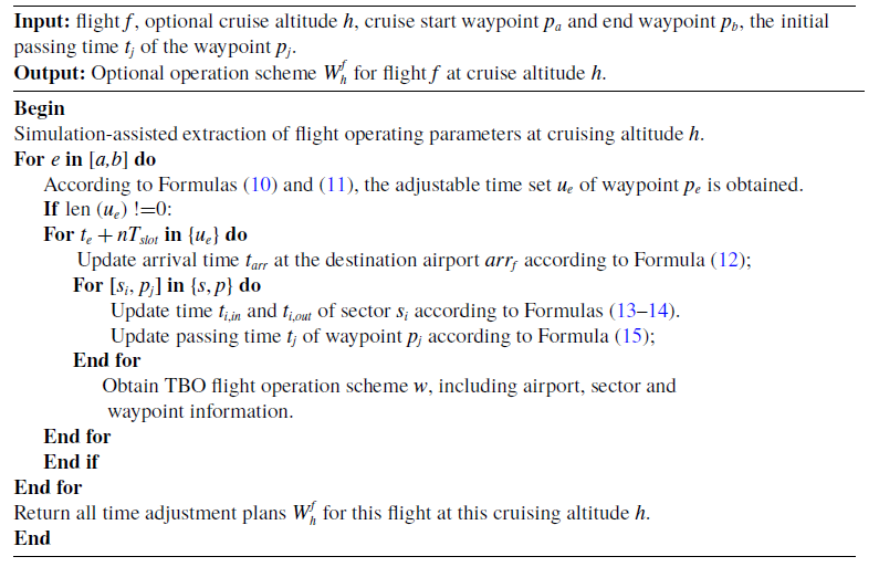The updated calculation methods for the operational times of the corresponding sectors ${s_i}$ , waypoints ${p_j}$ , and arrival airports $ar{r_f}$ after adjustment are described in Equations (14) to (17). The pseudocode for the TBO flight operation plan generation method is shown in Algorithm 2.

Algorithm 2:

TBO flight operation plan generation method

An equation showing flight operation plan generation method.

Algorithm 2: Long description

The equation describes the TBO flight operation plan generation method. It includes variables such as Vmin h and Vmax h, representing the minimum and maximum speeds of flight at cruising altitude h in meters per second. VW a e denotes the average wind speed between flight points p a and p e. The equation also involves a non-zero integer n, a waypoint timing factor chi, and an adjustable time interval theta. The adjustable time t e f minus t a f plus n T slot must fall within the interval theta for chi to equal 1, indicating achievable adjusted time by adjusting aircraft speed. If no such n exists, chi equals 0, indicating constraints due to aircraft performance. The minimum adjustable time slot duration T slot is set to 180 seconds. The equation transforms continuous optimization into a discrete problem solvable via integer linear programming, aligning with air traffic control operations. The final result is the set of time-adjustable schemes u e for waypoint p e.

The arrival time ${t_{arr}}$ at airport $ar{r_f}$ is:

(14)

\begin{align} {t_{arr}} = \left\{ {\begin{array}{l@{\quad}c}{{t_{arr}} + n{T_{{\rm{slot}}}}} & {}{if{\rm{ }}{t_{arr}} + nT \in {u_j}}\\[4pt]{{t_{arr}}} & {}{else}\end{array}} \right. \end{align}

The adjusted entry time ${t_{i,in}}$ for sector ${s_i}$ is:

(15)

StartLayout 1st Row t Subscript i comma i n Baseline equals StartLayout Enlarged left brace 1st Row t Subscript i comma i n Baseline plus n upper T Subscript normal s normal l normal o normal t Baseline t Subscript e Baseline less than t Subscript i comma i n Baseline 2nd Row t Subscript a Baseline plus left parenthesis t Subscript i comma i n Baseline minus t Subscript a Baseline right parenthesis times StartFraction t Subscript e Baseline minus t Subscript a Baseline plus n upper T Subscript normal s normal l normal o normal t Baseline Over t Subscript e Baseline minus t Subscript a Baseline EndFraction t Subscript a Baseline less than t Subscript i comma i n Baseline less than t Subscript e Baseline 3rd Row t Subscript i comma i n Baseline t Subscript i comma i n Baseline less than or equals t Subscript a Baseline EndLayout EndLayout

\begin{align} {t_{i,in}} = \left\{ {\begin{array}{c}{{t_{i,in}} + n{T_{{\rm{slot}}}}} \quad\quad\quad\quad\quad\quad\quad\quad\quad {{t_e} \lt {t_{i,in}}}\\[10pt]{{t_a} + ({t_{i,in}} - {t_a}) \times \dfrac{{{t_e} - {t_a} + n{T_{{\rm{slot}}}}}}{{{t_e} - {t_a}}}} {} \quad {{t_a} \lt {t_{i,in}} \lt {t_e}}\\[10pt]{{t_{i,in}}} \quad\quad\quad\quad\quad\quad\quad\quad\quad\quad\quad\quad {}{{t_{i,in}} \le {t_a}}\end{array}} \right. \end{align}

The adjusted exit time ${t_{i,out}}$ for sector ${s_i}$ is:

(16)

StartLayout 1st Row t Subscript i comma o u t Baseline equals StartLayout Enlarged left brace 1st Row t Subscript i comma o u t Baseline plus n upper T Subscript normal s normal l normal o normal t Baseline t Subscript e Baseline less than t Subscript i comma o u t Baseline 2nd Row t Subscript a Baseline plus left parenthesis t Subscript i comma o u t Baseline minus t Subscript a Baseline right parenthesis times StartFraction t Subscript e Baseline minus t Subscript a Baseline plus n upper T Subscript normal s normal l normal o normal t Baseline Over t Subscript e Baseline minus t Subscript a Baseline EndFraction t Subscript a Baseline less than t Subscript i comma o u t Baseline less than or equals t Subscript e Baseline 3rd Row t Subscript i comma o u t Baseline t Subscript i comma o u t Baseline less than or equals t Subscript a Baseline EndLayout EndLayout

\begin{align} {t_{i,out}} = \left\{ {\begin{array}{c}{{t_{i,out}} + n{T_{{\rm{slot}}}}} \quad\quad\quad\quad\quad\quad\quad\quad {}{{t_e} \lt {t_{i,out}}}\\[10pt]{{t_a} + ({t_{i,out}} - {t_a}) \times \dfrac{{{t_e} - {t_a} + n{T_{{\rm{slot}}}}}}{{{t_e} - {t_a}}}} {}\quad {{t_a} \lt {t_{i,out}} \le {t_e}}\\[10pt]{{t_{i,out}}} \quad\quad\quad\quad\quad\quad\quad\quad\quad\quad {}{{t_{i,out}} \le {t_a}}\end{array}} \right. \end{align}

The adjusted time ${t_j}$ of passing the waypoint ${p_j}$ is:

(17)

StartLayout 1st Row t Subscript j Baseline equals StartLayout Enlarged left brace 1st Row t Subscript j Baseline plus n upper T Subscript normal s normal l normal o normal t Baseline e less than j 2nd Row t Subscript a Baseline plus left parenthesis t Subscript j Baseline minus t Subscript a Baseline right parenthesis times StartFraction t Subscript e Baseline minus t Subscript a Baseline plus n upper T Subscript normal s normal l normal o normal t Baseline Over t Subscript e Baseline minus t Subscript a Baseline EndFraction a less than j less than or equals e 3rd Row t Subscript j Baseline j less than or equals a EndLayout EndLayout

\begin{align} {t_j} = \left\{ {\begin{array}{c}{{t_j} + n{T_{{\rm{slot}}}}} {}\quad\quad\quad\quad\quad\quad{e \lt j}\\[10pt]{{t_a} + ({t_j} - {t_a}) \times \dfrac{{{t_e} - {t_a} + n{T_{{\rm{slot}}}}}}{{{t_e} - {t_a}}}}\quad {}{a \lt j \le e}\\[10pt]{{t_j}} {}\quad\quad\quad\quad\quad\quad\quad\quad\quad\quad{j \le a}\end{array}} \right. \end{align}

4.3 Large-scale optimisation model of flight trajectory

This paper establishes a large-scale flight trajectory optimisation model operating at the pre-tactical level. The overall methodology and computational steps are illustrated in Fig. 8. Given the substantial number of variables and constraints inherent in large-scale optimisation problems, the following simplifying assumptions are adopted: (1) vertical wind effects on aircraft trajectory and performance are neglected, whereas horizontal wind effects on aircraft ground speed, track and fuel consumption are considered; (2) aircraft are modeled in clean configuration during optimisation; (3) statistical data indicate that Airbus A320, A321 and Boeing B737-800 aircraft types collectively account for over 60% of the fleet; consequently, only these three types constitute the set of available aircraft for flights. The remainder of this section details the optimisation model for flights under TBO, presenting its objective function, decision variables and constraints.

Figure 8.

Experimental framework for large-scale flight trajectory optimisation model.

A flowchart illustrating the stages of large-scale flight trajectory optimization model.

Figure 8 Long description

The flowchart illustrates the stages of large-scale flight trajectory optimization model. The process begins with the Initial National Flight Plan, which generates a TBO flight operation plan. This plan feeds into the Large-scale flight trajectory optimization model, which includes an objective function, optimization method, and constraints such as fuel consumption, cruise altitude, airspace capacity, time of aircraft passing through waypoints, airport capacity, and waypoint capacity. The model integrates data from the Atmosphere model, which includes temperature, pressure, and density; the Aircraft dynamics model, which includes speed limitation, height limitation, and aircraft state transition; the Waypoint capacity model, which includes flight level, en-route structure, and traffic flow distribution; and the Fuel consumption model, which includes fuel flow rate, fuel consumption, and thrust/drag. The output of the Large-scale flight trajectory optimization model is a Flight adjustment operation plan, which is then analyzed for optimization results.

4.3.1 Objective function

4.3.1.1 Objective function 1: Excess sector traffic flow

When the number of flights within a sector exceeds its capacity, it causes not only sector congestion and flight delays but also increases ATC workload. Therefore, the objective of the airspace traffic flow optimisation is to achieve a balanced spatiotemporal distribution of traffic flow, thereby mitigating sector congestion (as formalised in Equations (18) and (19)),

(18)

\begin{align} {F_1} &= \min \sum\limits_{s \in S,m \in M} {O_s^m} \\[-10pt] \nonumber\end{align}

(19)

StartLayout 1st Row 1st Column upper O Subscript s Superscript m 2nd Column equals max left parenthesis left parenthesis sigma summation Underscript StartLayout 1st Row f element of upper F comma s Subscript i Superscript f Baseline equals s comma 2nd Row t Subscript i comma i n Superscript f Baseline element of m comma t Subscript i comma o u t Superscript f Baseline element of m EndLayout Endscripts x Subscript k Superscript f Baseline right parenthesis minus upper C Subscript s Superscript m Baseline comma 0 right parenthesis EndLayout

\begin{align} O_{s}^{m} &= \max \left(\left(\sum\limits_{f \in F,s_{i}^{f} = s,\atop t_{i,in}^{f} \in m,t_{i,out}^f \in m} {x_{k}^{f}}\right) - C_{s}^{m},0\right) \\[8pt] \nonumber\end{align}

where $O_{\!s}^m$ is defined as the excess traffic in sector $s$ during time period $m$ . If the flight traffic in sector $s$ during time period $m$ exceeds the maximum capacity of the sector, it is considered that sector $s$ is congested during time period $m$ , and the excess traffic in sector $s$ is equal to the difference between the flight traffic in sector $s$ during time period $m$ and the maximum capacity of the sector; if the flight traffic is less than or equal to the maximum capacity of the sector, it is equal to 0. The optimisation horizon spans a 24-hour period. This period is discretised into 96 consecutive 15-minute time periods (e.g., 00:00–00:15, 00:15–00:30, …, 23:45–24:00, where 24:00 denotes the end of the period). The study airspace comprises 241 ATC sectors. This spatiotemporal discretisation facilitates the optimisation of traffic flows across both time and space dimensions.

4.3.1.2 Objective function 2: Cruise-phase fuel consumption

During a flight, the aircraft primarily operates in the cruise phase, where both the flight time and fuel consumption predominantly occur. Therefore, optimising fuel consumption during cruise is crucial for enhancing fuel efficiency and reducing emissions. To account for the impact of varying weather conditions, the cruise trajectory is discretised into segments defined by waypoints. The fuel consumption between adjacent waypoints is computed by iteratively summing incremental fuel burn estimates, as formalised in Equation (20).

(20)

\begin{align} {F_2} = \min \sum\limits_{f \in F,p_j^f \in {p^f}} {f{f_{p_j^f}} \cdot t_j^f} \end{align}

To reconcile the inherent trade-off between minimising sector flow exceedance and fuel consumption, we formulate a prioritised multi-objective optimisation problem. This is implemented using Gurobi’s hierarchical objective function (Model.setObjectiveN()). Sector flow exceedance cost is assigned the primary objective with higher priority, reflecting the paramount importance of airspace safety and capacity compliance. Fuel consumption is set as a secondary objective. The framework allows for a controlled trade-off by specifying tolerance parameters, which permit a bounded relaxation of the primary objective’s optimality to seek improvements in the secondary objective. This approach ensures that capacity constraints are first strictly satisfied, while efficiently exploring fuel-saving opportunities within defined operational margins.

4.3.2 Decision variables

The flight operation plan for a given flight serves as the decision variable, as shown in Equation (21). TBO flight operation plan generation methodology can generate a set of alternative plans for each flight to be optimised. This methodology was introduced in Section 4.2. However, in the operational context, only one plan per flight can be selected from its corresponding set.

(21)

\begin{align} x_k^f =\left\{\begin{matrix}1 &\quad \text{if flight } f \text{ selects the } k^{\text{th}} \text{ peration plan} \\[2pt]0 &\quad else \end{matrix}\right.\quad \forall f \in F,\; \forall k \in W_f \end{align}

4.3.3 Constraints

4.3.3.1 Airport arrival capacity constraints

Since the model treats the cruise altitude profile and waypoint overflight times of optimised flights as decision variables, it does not affect the departure time of flights but affects the total flight time. Consequently, constraints must be imposed on the arrival times of operation plans. To respect airport capacity limitations, the hourly arrival rate at any airport must not exceed its maximum capacity, as expressed in Formula (22).

(22)

\begin{align} \sum\limits_{a{\rm{r}}{{\rm{r}}_{_f}} = q,t_{arr}^f \in m} {x_k^f \le C_q^n} ,\forall f \in F,\forall m \in M,\forall q \in Q,k \in {W_f} \end{align}

4.3.3.2 Waypoint capacity constraints

In operational air traffic management, waypoint capacity represents a critical metric directly influencing the safety and efficiency of the en-route network. When the peak traffic volume exceeds the rated capacity of a waypoint, it signifies an inefficient or potentially unsafe distribution of traffic flow during that period. Therefore, constraining the traffic flow during peak hours within congested altitude bands at waypoints is essential, as expressed in Formula (23). The model for assessing waypoint capacity is presented in Section 3.

(23)

\begin{align} \sum\limits_{p_j^f = p,t_j^f \in m,h_j^f = h} {x_k^f \le C_p^{m,h},} \forall f \in F,\forall p \in P,h \in H,m \in M \end{align}

5.0 Experiments

5.1 Data

5.1.1 Flight trajectory data

In actual air operations, flight trajectories are significantly influenced by seasonal factors and air traffic control procedures. For flights operating between the same city pairs, controllers routinely assign specific cruising altitudes to aircraft, directing them to execute climb or descent operations after passing designated waypoints. Therefore, this study selects historical radar data of all Chinese flights from August 1 to 31, 2018 to extract regularity feature of flight paths and altitude profiles between city pairs, while extracting operational feature of waypoints from historical peak traffic flow data at these waypoints. The large-scale flight trajectory optimisation experiment employed the complete flight schedule of Chinese domestic operations (all flights with both departure and arrival airports within China) from August 13, 2018, totaling 9494 flights as the subject for optimisation. These flight operations data, together with European Centre for Medium-Range Weather Forecasts Re-Analysis 5 (ERA5) meteorological data, were integrated as authentic data sources and fed into the ATOSS for simulation and parameter extraction, which subsequently served as input parameters for the optimisation model.

5.1.2 ERA5 Meteorological data

European Centre for Medium-Range Weather Forecasts Re-Analysis 5 (ERA5) is the fifth-generation atmospheric reanalysis dataset developed by European Centre for Medium-Range Weather Forecasts (ECMWF), providing comprehensive global climate records from January 1950 to present [Reference Hersbach, Bell and Berrisford49]. The ERA5 dataset employed in this experiment covers the date of August 13, 2018, with a spatial resolution of $0.25^\circ \times 0.25^\circ $ and a temporal resolution of 1 hour. 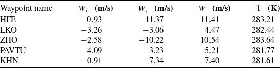The study primarily utilises parameter values including ${W_x}$ component, ${W_y}$ wind component, and temperature $T$ at various pressure levels within Chinese longitudinal and latitudinal regions for each hourly time step. Since the ERA5 dataset provides parameter values across 37 pressure levels at 24-hour intervals, the initial processing involves: variable conversion between atmospheric temperature, pressure altitude and true altitude using the standard atmospheric model from BADA; and bilinear interpolation of ERA5 data based on waypoint coordinates. This yields meteorological data for each waypoint at different flight levels during different time periods, as detailed in Table 3.

Table 3.

Weather conditions at waypoints (2018.8.13,14:00–15:00,7,800 m)

A table showing weather conditions at various waypoints on August 13, 2018, at 7,800 meters altitude.

Table 3 Long description

The table presents weather conditions at different waypoints on August 13, 2018, between 14:00 and 15:00 at an altitude of 7,800 meters. It includes data for five waypoints: HFE, LKO, ZHO, PAVTU, and KHN. The table has five rows and four columns. The columns are labeled with the waypoint names and the variables Wx, Wy, W, and T. Wx and Wy represent wind components in meters per second, W represents the total wind speed in meters per second, and T represents the temperature in Kelvin. Row 1: HFE, Wx 0.93 meters per second, Wy 11.37 meters per second, W 11.41 meters per second, T 283.21 Kelvin. Row 2: LKO, Wx -3.26 meters per second, Wy -3.06 meters per second, W 4.47 meters per second, T 282.44 Kelvin. Row 3: ZHO, Wx -2.58 meters per second, Wy -10.22 meters per second, W 10.54 meters per second, T 283.64 Kelvin. Row 4: PAVTU, Wx -4.09 meters per second, Wy -3.23 meters per second, W 5.21 meters per second, T 281.77 Kelvin. Row 5: KHN, Wx -0.91 meters per second, Wy 7.34 meters per second, W 7.40 meters per second, T 281.61 Kelvin.

5.2 Experimental environment

The flight plan simulation in this study was conducted using the air traffic operation simulation system (ATOSS), independently developed by the New Generation Intelligent Air Traffic Control Research Laboratory at Nanjing University of Aeronautics and Astronautics (NUAA). ATOSS is a cloud-based simulation system that rapidly models air traffic networks based on user demands, supports flexible operation scheme configurations, enables fast simulations.

Figure 9.

ATOSS interface display.

Figure 9 Long description

A heat map displaying flight routes and air traffic management data across a region. The map shows a network of interconnected flight paths with varying intensities of traffic. The color scale indicates the level of air traffic, with darker colors representing higher traffic density. Key data points include specific coordinates, altitude levels, and time periods for flights. The map also highlights areas with excess traffic flow and capacity constraints in different sectors and airports. Various symbols and annotations provide additional details about flight levels, waypoints, and timing adjustments. The overall structure includes a grid layout with labeled axes representing geographical coordinates and time periods. The data is used for analyzing and optimizing air traffic control strategies.

The hardware environment for the experiment is HP Z8-G4 workstation (configured with one Intel Xeon(R) Gold 6,242 CPU and 64GB RAM). The software environment was based on a 64-bit Windows 7 operating system and utilised Gurobi version 10.0.1. The experimental process was conducted using Python 3.7.

5.3 Case analysis

5.3.1 Waypoint capacity evaluation results

To validate the reliability of our proposed simulation waypoint capacity assessment method, we verify whether single-altitude-layer capacity assessments satisfy operational requirements. Since existing studies primarily evaluate hourly capacity at ATC waypoints, we compare simulated hourly capacities at single-altitude layers against historical peak-hour traffic data. Comparative analysis of these differences validates our waypoint capacity assessment methodology. Two high-density waypoints (HFE and P263) serve as case studies, with capacity assessed across multiple altitude layers. Figure 10 presents comparative results of simulated versus observed capacities.

Table 4.

ZGSZ-ZSSS city flight altitude profile clustering result

A table showing clustering results for ZGSZ-ZSSS city flight altitude profiles, including cluster sizes and silhouette coefficients.

Table 4 Long description

The table presents clustering results for ZGSZ-ZSSS city flight altitude profiles. It includes five columns: Cluster 1, Cluster 2, Cluster 3, Cluster 4, and Noise, with a total row. The table has two rows of data: Size and Silhouette coefficient. Cluster 1 has a size of 22 and a silhouette coefficient of 0.697. Cluster 2 has a size of 25 and a silhouette coefficient of 0.878. Cluster 3 has a size of 43 and a silhouette coefficient of 0.6. Cluster 4 has a size of 49 and a silhouette coefficient of 0.668. The Noise row has a size of 13 and no silhouette coefficient. The total size across all clusters and noise is 152.

Figure 10.

Validation of historical data on waypoint capacity. (a) Waypoint HFE. (b) Waypoint P263.

A bar graph compares hourly capacity at different flight levels for two waypoints, HFE and P263, using simulation evaluation methods and historical peak data.

Figure 10 Long description

The bar graph compares hourly capacity at different flight levels for two waypoints, HFE and P263. The x-axis represents flight levels in meters, and the y-axis represents hourly capacity in flights per hour. Each waypoint has two sets of bars: one for simulation evaluation methods in red and one for historical peak data in blue. For waypoint HFE, flight levels are 6300, 7200, 8100, and 9800 meters. For waypoint P263, flight levels are 8400, 8900, 9200, and 9800 meters. The historical peak data generally shows higher capacity than the simulation evaluation methods. All values are approximated.

Figure 10 reveals that our waypoint capacity evaluations yield conservative estimates relative to historical peak traffic. This conservatism stems from incorporating controller workload factors (e.g. headway distribution) and stringent safety constraints (separation distance L), producing capacity estimates more reflective of operational realities. Furthermore, historical peaks reflect context-specific achievements, lacking generalisability across diverse operational scenarios. Conversely, our methodology demonstrates superior robustness, safety and universality by systematically quantifying operational constraints and risk exposure.

5.3.2 Flight altitude profile clustering results

Using flights between ZGSZ and ZSSS as a case study, we extracted and clustered 152 altitude profiles (Fig. 11). Pairwise profile similarity was computed using Equations (10) and (11). Subsequently, we applied the DBSCAN algorithm across a range of parameter combinations (ε, minPts) for clustering. For each resulting clustering, the corresponding silhouette coefficient was calculated. The mean silhouette coefficient, $\ell $ , ranges from [−1, 1], with higher values indicating better-defined clusters.

Figure 11.

ZGSZ-ZSSS city flight altitude profile.

A line graph showing flight altitude in meters against flight distance in kilometers.

Figure 11 Long description

A line graph displays multiple flight altitude profiles over a flight distance. The x-axis represents flight distance in kilometers, ranging from 0 to 1200 kilometers. The y-axis represents flight altitude in meters, ranging from 0 to 13000 meters. Each line represents a different flight, showing how the altitude changes over the distance. The flights generally start at a lower altitude, increase to a cruising altitude between 9000 and 11000 meters, and then descend towards the end of the flight distance. All values are approximated.

Following iterative evaluation, the optimal DBSCAN parameters were determined as ε = 600 and minPts = 15. The resulting clustering (Fig. 12) produced four well-defined clusters comprising 22, 25, 43 and 49 altitude profiles, respectively, with 13 outliers removed. The corresponding mean silhouette coefficients for each cluster are presented in Table 4. The overall mean silhouette coefficient ( $\ell $ = 0.69) exceeds the threshold of 0.5, confirming a robust and well-separated cluster structure and validating the effectiveness of the DBSCAN algorithm for this application.

Figure 12.

ZGSZ-ZSSS city flight altitude clustering profile. (a) The first set of altitude clustering profile. (b) The second set of altitude clustering profile. (c) The third set of altitude clustering profile. (d) The fourth set of altitude clustering profile.

Four line graphs depict flight altitude clustering profiles for different sets of flights between two cities.

Figure 12 Long description

The image contains four line graphs labeled (a), (b), (c), and (d), each representing a different set of altitude clustering profiles for flights between two cities. Each graph plots flight altitude in meters on the y-axis against flight distance in kilometers on the x-axis. Graph (a), in green, shows the first set of altitude clustering profiles, with multiple lines indicating various flight paths. Graph (b), in orange, represents the second set, showing a similar pattern with flights reaching altitudes up to 12000 meters. Graph (c), in purple, illustrates the third set, with flights also reaching up to 12000 meters. Graph (d), in red, depicts the fourth set, following a comparable pattern. Each graph shows flights initially ascending, maintaining a cruising altitude, and then descending towards the destination. The lines in each graph represent individual flight paths, with variations in altitude and distance. All values are approximated.

5.3.3 Flight trajectory optimisation results

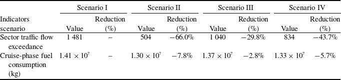
To assess congestion mitigation effectiveness of the proposed optimisation methods, we analyse sector overload reduction and fuel savings independently while evaluating trajectory modifications. Two scenarios are compared: Scenario I (initial scenario, the simulated operational state based on the original flight schedules) and Scenario II (TBO scenario). Table 5 presents performance metrics for both scenarios. Sector overload decreased by 976 flights (66.0%) under TBO optimisation. Cruise-phase fuel consumption reduced by 0.11 × 10⁷ kg (7.8%). These results demonstrate the model’s effectiveness in reducing sector congestion and improving fuel efficiency.

5.3.3.1 Traffic flow result

Temporally, Fig. 13 depicts the variations in total excess traffic across all sectors prior to and following optimisation. Following optimisation, sector congestion was significantly reduced, with improvements evident across all time periods. Prior to optimisation, the periods of most pronounced congestion occurred at 13:00–15:00 and 18:00–20:00. Although peak periods persist post-optimisation, both the duration and peak congestion values in the TBO scenario were significantly reduced. This demonstrates that adjusting flight altitudes and regulating waypoint overflight times can effectively mitigate sector congestion, preventing excessively severe localised congestion and effectively regulating dense air traffic flows during peak hours.

Table 5.

Operational plan optimisation indicator results

Table 5 Long description

The table presents statistical indicators for sector traffic flow exceedance and cruise-phase fuel consumption across two scenarios: initial and TBO. It includes three columns: Statistical indicators, Initial scenario, TBO scenario, and Optimisation percentage. The first row shows sector traffic flow exceedance with values 1481 for the initial scenario, 504 for the TBO scenario, and an optimisation percentage of negative 66.0 percent. The second row displays cruise-phase fuel consumption in kilograms, with values 1.41 times 10 to the power of 7 for the initial scenario, 1.30 times 10 to the power of 7 for the TBO scenario, and an optimisation percentage of negative 7.8 percent. The table highlights significant reductions in both sector traffic flow exceedance and cruise-phase fuel consumption under the TBO scenario.

Figure 13.

Total excess sector traffic flow under different time periods.

A line graph showing total sectors excess traffic flow under different time periods.

Figure 13 Long description

The line graph displays total sectors excess traffic flow under different time periods. The x axis represents time periods in 15-minute intervals from 8:00 to 23:15. The y axis represents the total sectors excess traffic flow, ranging from 0 to 50. Two data series are shown: the initial scenario in red and the TBO scenario in blue. The graph indicates fluctuations in traffic flow throughout the day, with peaks and troughs at various times. The initial scenario generally shows higher excess traffic flow compared to the TBO scenario. All values are approximated.

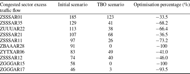
Spatially, the congestion levels across congested sectors throughout the day are presented in Fig. 14 and Table 6. Following optimisation, sector congestion was significantly alleviated. For instance, sectors like ZBAAAR28, ZGGGAR15 and ZSSSAR23 were completely free of congestion post-optimisation, and traffic flow distribution became more balanced; while others, including ZSSSAR35 and ZUUUAR22, exhibited congestion reduction rates exceeding 60%, indicating substantial mitigation; however, residual congestion persisted in sectors such as ZSSSAR01 and ZSSSAR21. To further mitigate congestion in these sectors, strategic ground delay measures may be required to reschedule the departure times of affected flights.

Table 6.

Optimisation results for excess traffic flow in congested sectors

Table comparing initial and optimized traffic flow scenarios in congested sectors with optimization percentages.

Table 6 Long description

A table with 10 rows and 4 columns presents data on the optimization results for excess traffic flow in congested sectors. The columns are labeled Congested sector excess traffic flow, Initial scenario, TBO scenario, and Optimization percentage (percentage). Each row lists a specific sector, its initial traffic flow, the traffic flow after optimization, and the percentage of optimization achieved. Notable trends include sectors like ZBAAAR28 and ZGGGAR15 achieving 100% optimization, while others like ZSSSAR01 and ZSSSAR21 show significant but incomplete reductions in congestion. The data highlights varying degrees of congestion alleviation across different sectors.

Figure 14.

Total time period excess traffic flow under different sectors.

Figure 14 Long description

The bar graph compares total time period excess traffic flow under different sectors for two scenarios, Initial scenario and T B O scenario. The x-axis represents the sectors, labeled as Z S S S A R 01, Z S S S A R 35, Z U U U A R 22, Z S S S A R 21, Z S S S A R 11, Z B A A R 28, Z Y T X A R 06, Z S S S A R 12, Z G G G A R 15, Z G G G A R 17, Z U U U A R 12, Z S S S A R 23, Z S S S A R 36, Z Y T L A R 02. The y-axis represents the total time period excess traffic flow, ranging from 0 to 200. The graph features two sets of bars for each sector: one in red representing the Initial scenario and one in blue representing the T B O scenario. Notable trends include higher excess traffic flow in the Initial scenario for most sectors, with significant differences observed in sectors like Z S S S A R 01 and Z S S S A R 35. The T B O scenario generally shows lower excess traffic flow across sectors. All values are approximated.

To quantify the imbalance in the spatiotemporal distribution of excess flight traffic, we introduce the following two metrics:

• Number of excess time periods: This refers to the number of time periods within a single sector that have an excess flow.
• Number of excess sectors: This refers to the number of sectors during a single time period that have an excess flow.

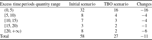
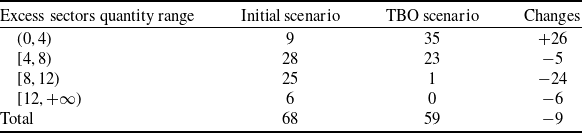
By analysing the distribution of all excess sector counts and excess time period counts, the optimisation of excess traffic is obtained as shown in Tables 7 and 8. The principle behind the reallocation of airspace traffic flow in this paper is to transfer the flight traffic of a sector to other time periods before or after the sector or to the same time period in spatially adjacent sectors. As shown in Fig. 15(a), the count of excess time periods per sector exhibits an overall declining trend, with the total occurrences of sector congestion reduced by 53.4% post-optimisation. Figure 15(b) demonstrates that the distribution of congested sectors per time slot shifts markedly leftward after optimisation, evidenced by the decrease in time periods experiencing more than 8 congested sectors from 32 to 1, indicating that the proposed method effectively alleviates congestion imbalances across both temporal and spatial dimensions. However, due to inherent constraints, such as aircraft performance limitations, flight transit times, and bounds on feasible altitude profile adjustments, residual congestion persists in certain time periods within congested sectors.

Table 7.

Results distribution of number of excess periods

A table showing the distribution of excess time periods in an initial scenario and a TBO scenario.

Table 7 Long description

The table presents the distribution of excess time periods across different quantity ranges, comparing an initial scenario with a TBO scenario. It includes five rows for different ranges of excess time periods: (0, 5), [5, 10), [10, 15), [15, 20), and [20, +∞). Each row shows the quantity of excess time periods in the initial scenario, the TBO scenario, and the changes between the two scenarios. The total number of excess time periods decreases from 58 in the initial scenario to 27 in the TBO scenario, indicating an overall reduction of 11. Notable changes include a significant decrease in the (0, 5) range from 32 to 16 and in the [20, +∞) range from 8 to 2.

Table 8.

Results distribution of number of excess sectors

A table comparing the distribution of excess sectors quantity range across initial and TBO scenarios, showing changes in sector congestion.

Table 8 Long description

The table presents the distribution of excess sectors quantity range across initial and TBO scenarios, highlighting the changes in sector congestion. It consists of four rows and four columns. The columns are labeled 'Excess sectors quantity range', 'Initial scenario', 'TBO scenario', and 'Changes'. The rows are labeled with different ranges of excess sectors: (0, 4), [4, 8), [8, 12), and [12, +∞). The table shows that for the range (0, 4), the initial scenario had 9 instances, which increased to 35 in the TBO scenario, a change of +26. For the range [4, 8), the initial scenario had 28 instances, which decreased to 23 in the TBO scenario, a change of -5. For the range [8, 12), the initial scenario had 25 instances, which dropped significantly to 1 in the TBO scenario, a change of -24. For the range [12, +∞), the initial scenario had 6 instances, which decreased to 0 in the TBO scenario, a change of -6. The total number of excess sectors decreased from 68 in the initial scenario to 59 in the TBO scenario, a change of -9. This table illustrates the overall reduction in sector congestion post-optimization, with notable decreases in higher ranges of excess sectors.

Figure 15.

Distribution of excess traffic flow optimisation. (a) Distribution of number of excess periods. (b) Distribution of number of excess sectors.

A histogram showing the distribution of excess traffic flow optimization in two scenarios.

Figure 15 Long description

The histogram consists of two subplots labeled (a) and (b). Subplot (a) shows the distribution of the number of excess periods, with the x-axis representing the number of excess time periods and the y-axis representing frequency. The data is divided into vertical bars, with red bars representing the initial scenario and blue bars representing the TBO scenario. The distribution shows a higher frequency of excess periods in the initial scenario compared to the TBO scenario. Subplot (b) shows the distribution of the number of excess sectors, with the x-axis representing the number of excess sectors and the y-axis representing frequency. Similar to subplot (a), red bars represent the initial scenario and blue bars represent the TBO scenario. The distribution indicates a shift in the number of excess sectors between the two scenarios. Both subplots include smooth curves that represent the overall distribution trends. The data is continuous, and the values are approximated.

Integrating temporal and spatial dimensions, the congestion levels of the top ten busiest sectors before and after optimisation are depicted in Figs 16–17, while detailed traffic flow patterns for selected busy sectors are illustrated in Fig. 18. Prior to optimisation, persistent congestion spanning consecutive time periods was observed in several sectors, severely impeding the rational allocation of airspace resources. Notable examples include sector ZBAAAR28 during 7:00–10:00 and sector ZSSSAR17 during 13:00–16:00. Following optimisation, flight counts in the majority of time periods across busy sectors fell below sector capacity, and excessive congestion was largely eliminated, resulting in a significant overall improvement. In the limited sectors and time periods where residual congestion persists post-optimisation, the magnitude of excess traffic was substantially lower than pre-optimisation levels, and such short-duration congestion events were distributed more evenly across time periods and sectors.

Figure 16.

Initial scenario of excess flow in the top ten congested sectors.

A heat map showing excess flow in the top ten congested sectors over time periods.

Figure 16 Long description

A heat map displays excess flow in the top ten congested sectors over various time periods. The map uses a grid layout with sectors listed on the vertical axis and time periods on the horizontal axis. The color scale ranges from light yellow to dark purple, indicating increasing levels of excess flow. Higher values are represented by darker colors. The heat map shows specific values within each cell, highlighting areas of congestion. Notable clusters of high excess flow are visible during certain time periods, particularly in the late afternoon and early evening. The data represents actual measurements of traffic flow in these sectors.

Figure 17.

TBO scenario of excess flow in the top ten congested sectors.

Figure 17 Long description

A heat map displays excess traffic flow in top ten congested sectors over time periods. The heat map is structured as a grid with sectors listed vertically and time periods horizontally. The color scale ranges from light yellow to dark purple, indicating increasing levels of excess traffic flow. Darker colors represent higher values of excess traffic flow, while lighter colors indicate lower values. The map shows specific values within each cell, with some cells containing multiple values. Notable regions of high excess traffic flow are observed at various time periods across different sectors. The data is actual and reflects the TBO scenario of excess flow in the top ten congested sectors.

5.3.3.2 Fuel consumption result

Statistical analysis of the optimisation results, categorised by flight distance, is presented in Table 9 and Fig. 19(a). Most flights nationwide are medium- to short-haul flights with a flight distance of less than 2,000 km, while flights exceeding 2,000 km account for only 7.2% of the total number of flights nationwide. Figure 19(a) reveals a positive correlation between fuel consumption and flight distance. Furthermore, per-flight fuel savings are positively correlated with flight distance. As a result, long-haul flights should be prioritised as primary optimisation targets when selecting a subset, given their larger potential for fuel savings.

Table 9.

Flight distance optimisation statistics results

A table comparing flight distance optimization statistics, including fuel consumption and number of flights.

Table 9 Long description

The table presents flight distance optimization statistics, categorized by flight distance ranges in meters. It includes columns for initial scenario fuel consumption in kilograms, TBO scenario fuel consumption in kilograms, number of flights, and average fuel reduction in kilograms per flight. The table has five rows, each representing a different flight distance range: (0, 1000], (1000, 1500], (1500, 2000], (2000, 2500], and (2500, +∞). Notable trends include a positive correlation between flight distance and average fuel reduction, with longer flight distances showing higher fuel savings per flight. For example, flights in the (2500, +∞) range have the highest average fuel reduction of 449.3 kilograms per flight, while flights in the (0, 1000] range have the lowest at 66.4 kilograms per flight.

Figure 18.

Flight traffic flow situation of busy sectors. (a) ZBAAAR28 sector. (b) ZGGGAR15 sector. (c) ZGGGAR17 sector. (d) ZGGGAR12 sector.

Four line graphs depict flight traffic flow in busy sectors over time periods, comparing initial and TBO scenarios against sector capacity.

Figure 18 Long description

The image contains four line graphs labeled (a) to (d), each representing flight traffic flow in different busy sectors over time periods. Each graph compares the initial scenario and TBO scenario against the sector capacity. The x-axis represents the time period, while the y-axis represents the flight traffic flow. The red line indicates the initial scenario, the blue line represents the TBO scenario, and the black dashed line shows the sector capacity. Graph (a) shows the ZBAAAR28 sector, graph (b) shows the ZGGGAR15 sector, graph (c) shows the ZGGGAR17 sector, and graph (d) shows the ZGGGAR12 sector. Each graph illustrates how flight traffic flow varies over time and compares it to the sector's capacity, highlighting periods where traffic flow exceeds or remains below the capacity. All values are approximated.

Optimisation of cruise altitudes was performed, and the results are summarised in Table 10 and Fig. 19(b). Prior to optimisation, the cruise altitudes of most flights were concentrated between (8,000, 10,000] m. Following optimisation, the cruise altitudes of most flights increased, indicating that cruise altitude significantly influences fuel consumption optimisation outcomes. When comparing fuel savings across different altitude ranges, cruise altitudes set between (9,000, 11,000] m yield greater fuel savings compared to other intervals. However, fuel savings do not increase monotonically with increasing cruise altitude; specifically, the savings achieved at altitudes above 11,000 m are less pronounced than those attained within the (9,000, 11,000] m range.

Table 10.

Flight altitude optimisation statistics results

A table comparing fuel consumption and savings across different cruising altitudes.

Table 10 Long description

The table presents data on fuel consumption and savings for flights at various cruising altitudes. It includes five rows and four columns. The columns are labeled as Cruising altitude (meters), Initial scenario fuel consumption (kilograms), TBO scenario fuel consumption (kilograms), and Average fuel reduction (kilograms per flight). The rows detail the data for different altitude ranges: (6000, 8000] meters, (8000, 9000] meters, (9000, 10000] meters, (10000, 11000] meters, and (11000, 13000] meters. Notable trends include significant fuel savings at higher altitudes, particularly between (9000, 11000] meters, where the average fuel reduction is highest at 214.9 kilograms per flight. However, fuel savings do not increase monotonically with altitude, as savings above 11000 meters are less pronounced.

Figure 19.

Fuel optimisation statistics results. (a) Fuel optimisation based on flight distance. (b) Fuel optimisation based on flight altitude.

Two bar graphs and one line graph depict fuel optimization statistics results based on flight distance and flight altitude.

Figure 19 Long description

The image contains two separate graphs labeled (a) and (b). Graph (a) shows fuel optimization based on flight distance, with two vertical bar graphs and one line graph. The x-axis represents cruising altitude in kilometers, divided into intervals such as (6000, 8000), (8000, 9000), and so on. The left y-axis shows the percentage of flights, while the right y-axis indicates average fuel reduction in kilograms per flight. The bar graphs compare the initial scene and TBO scenario across different cruising altitudes. The line graph represents the average fuel reduction, showing a peak around the (10000, 11000) kilometer interval. Graph (b) illustrates fuel optimization based on flight altitude, featuring one vertical bar graph and one line graph. The x-axis represents flight distance in kilometers, divided into intervals such as (0, 1000), (1000, 1500), and so on. The left y-axis shows the number of flights, while the right y-axis indicates average fuel reduction in kilograms per flight. The bar graph displays the number of flights within each distance interval, while the line graph shows the average fuel reduction, which increases significantly with longer flight distances. All values are approximated.

We statistically analysed optimisation results by city pair. As shown in Table 11, for city pairs including ZUUU-ZBAA and ZSSS-ZBAA, the average fuel savings per aircraft after optimisation were 42.4 kg and 9.3 kg, respectively. This suggests that the initial flight profiles for these city pairs were appropriately configured with limited scope for further optimisation. Consequently, for city pairs including ZBAA-ZGSZ and ZGGG-ZBAA, the average fuel savings reached 193.0 kg and 127.5 kg, respectively, demonstrating significant optimisation potential. This implies that the initial flight profiles were suboptimal, and these routes should be prioritised for flight profile optimisation in subsequent iterations.

To illustrate flight path adjustments, consider flight CCA1478 (ZBAA to ZWWW). Initially, the cruise altitude was 9,800 m with fuel consumption of 4784.3 kg. After optimisation, the cruise altitude increased to 10,300 m. Red markers indicate waypoints with time adjustments, blue markers denote waypoints with modified overflight times and black markers identify unaffected waypoints. Considering meteorological conditions and airspace constraints, the optimised profile (Fig. 20) achieved 4456.4 kg fuel consumption, representing a 327.9 kg (6.85%) reduction.

We categorised pre- and post-optimisation fuel consumption by aircraft type: A320, A321 and B737-800 (B738) accounted for 3369, 1650 and 4445 flights, representing 35.6, 17.4, and 47.0% of all flights, respectively. Using ICAO’s engine emission indices, we calculated emission reductions (Table 12). Through optimised flight time control and cruise altitude adjustments, total fuel savings reached $1.15 \times10^6$ kg, equivalent to emission reductions of 3.64 × 10⁶ kgCO₂, 1.15 × 10⁵gHC, 5.69 × 10⁵gCO, and 2.39 × 10⁷g NO_x.

Table 11.

Flight city-pair fuel optimisation statistics results

Table comparing fuel consumption and savings for different flight city pairs.

Table 11 Long description

A table with eight rows and four columns presents data on fuel consumption and savings for various flight city pairs. The columns are labeled Initial scenario fuel consumption, TBO scenario fuel consumption, Number of flights, and Average fuel reduction. The rows list different city pairs along with their respective data. Notable city pairs include ZBAA-ZSSS with an average fuel reduction of 56.4 kilograms per flight and ZBAA-ZGSZ with the highest reduction of 193.0 kilograms per flight. The table highlights significant fuel savings potential for certain routes, indicating suboptimal initial flight profiles.

Table 12.

Pollutant emissions optimisation statistics results

A table comparing fuel consumption and emission reductions for different aircraft types, including A320, A321, and B738, with data on fuel reduction, carbon dioxide, hydrocarbon, carbon monoxide, and nitrogen oxides emissions.

Table 12 Long description

The table presents data on fuel consumption and emission reductions for three aircraft types: A320, A321, and B738. It includes the number of flights, fuel reduction in kilograms, and reductions in emissions of carbon dioxide, hydrocarbon, carbon monoxide, and nitrogen oxides. The A320 had 3,369 flights with a fuel reduction of 4.18 times 10 to the power of 5 kilograms, resulting in emission reductions of 1.32 times 10 to the power of 6 kilograms of carbon dioxide, 8.36 times 10 to the power of 4 grams of hydrocarbon, 3.76 times 10 to the power of 5 grams of carbon monoxide, and 8.82 times 10 to the power of 6 grams of nitrogen oxides. The A321 had 1,650 flights with a fuel reduction of 2.04 times 10 to the power of 5 kilograms, resulting in emission reductions of 6.43 times 10 to the power of 5 kilograms of carbon dioxide, 2.04 times 10 to the power of 4 grams of hydrocarbon, 1.02 times 10 to the power of 5 grams of carbon monoxide, and 5.54 times 10 to the power of 6 grams of nitrogen oxides. The B738 had 4,445 flights with a fuel reduction of 5.33 times 10 to the power of 5 kilograms, resulting in emission reductions of 1.68 times 10 to the power of 6 kilograms of carbon dioxide, 1.07 times 10 to the power of 4 grams of hydrocarbon, 9.05 times 10 to the power of 4 grams of carbon monoxide, and 9.53 times 10 to the power of 6 grams of nitrogen oxides. In total, there were 9,464 flights with a fuel reduction of 1.15 times 10 to the power of 6 kilograms, resulting in emission reductions of 3.64 times 10 to the power of 6 kilograms of carbon dioxide, 1.15 times 10 to the power of 5 grams of hydrocarbon, 5.68 times 10 to the power of 5 grams of carbon monoxide, and 2.39 times 10 to the power of 7 grams of nitrogen oxides.

Figure 20.

Flight CCA1478 flight trajectory. (a) Initial flight trajectory. (b) TBO flight trajectory.

Two line graphs showing flight trajectories with waypoints and times.

Figure 20 Long description

Two line graphs compare initial and TBO flight trajectories for flight CCA1478. The x-axis represents distance, while the y-axis represents height. Each graph plots waypoints with corresponding times. The initial flight trajectory shows an original cruise height of ninety-eight hundred meters and original cruise fuel of four thousand seven hundred eighty-four point three kilograms. The TBO flight trajectory shows an optimal cruise height of ten thousand four hundred meters and optimal cruise fuel of four thousand four hundred fifty-six point four kilograms. Key waypoints include ZBAA, SOSDI, ANLOO, BEGRI, AKUKI, BAVU, DOTOS, ATBVG, GOVSA, ODURU, AGOXA, FKG, ZWWW, QTV, and others, each with specific times and heights. All values are approximated.

5.3.3.3 Comparative analysis

To benchmark the effectiveness of our proposed model, we introduced two additional experimental scenarios for comparison: (III) flight speed adjustment and (IV) flight altitude adjustment. The comparative performance indicators across all scenarios are summarised in Table 13. The results indicate that while all scenarios effectively alleviate airspace congestion and reduce fuel consumption, the TBO method achieves a substantially greater degree of improvement. Specifically, under identical experimental conditions, the TBO model reduced sector traffic flow exceedance by an additional 536 and 330 flights compared to scenarios III and IV, respectively. It also achieved extra fuel savings of 0.7 × 10⁷ and 0.3 × 10⁷ kg, respectively. The results demonstrate that the coordinated optimisation of altitude profiles and waypoint overflight times under the TBO mode is more effective than individual strategies, thereby highlighting the superiority of the model’s algorithm.

Table 13.

Indicator results of different optimization models

Table 13 Long description

The table presents a comparison of indicator results for four different optimization models. It includes data on sector traffic flow exceedance and cruise-phase fuel consumption across four scenarios. The table has four columns for each scenario and two rows for the indicators. Scenario I shows values of 1481 for sector traffic flow exceedance and 1.41 times 10 to the power of 7 kilograms for cruise-phase fuel consumption. Scenario II shows values of 504 for sector traffic flow exceedance, a reduction of 66 percentage, and 1.30 times 10 to the power of 7 kilograms for cruise-phase fuel consumption, a reduction of 7.8 percentage. Scenario III shows values of 1040 for sector traffic flow exceedance, a reduction of 29.8 percentage, and 1.37 times 10 to the power of 7 kilograms for cruise-phase fuel consumption, a reduction of 2.8 percentage. Scenario IV shows values of 834 for sector traffic flow exceedance, a reduction of 43.7 percentage, and 1.33 times 10 to the power of 7 kilograms for cruise-phase fuel consumption, a reduction of 5.7 percentage.

Computational efficiency is a critical performance metric for ATFM, particularly for large-scale optimisation problems. As the problem dimension scales, optimisation costs (e.g., computation time) typically increase exponentially, posing a significant challenge to algorithmic scalability and solver efficiency. To evaluate the algorithm’s scalability, experiments were designed across four traffic scales: (a) a single airport (e.g., ZBAA); (b) a subset of critical airports (the ten busiest in China); (c) all domestic flights on a given day; and (d) the average of all domestic flights over a week. As shown in the experimental results of Table 14, although the total flight volume at ZBAA in scenario (a) accounts for only one-tenth of the daily flight volume compared to scenario (c), these flights exert a remarkably strong influence on the optimisation outcome. In scenario (b), the total flights at the busiest airport cluster constitute about half of the daily volume, yet the optimisation result remains essentially consistent with the system-wide optimisation. This indicates that busy airports are often the primary cause of both airspace congestion and unnecessary fuel burn. To reduce time costs and improve optimisation efficiency, flight movements at busy airports should therefore warrant particular attention.

Table 14.

Indicator results of different optimization targets

A table comparing computational efficiency metrics across four traffic scenarios for air traffic flow management.

Table 14 Long description

The table presents indicator results of different optimization targets for air traffic flow management (ATFM) across four scenarios. It includes four columns for each scenario and four rows for different indicators. The columns are labeled Scenario a, Scenario b, Scenario c, and Scenario d. The rows are labeled Number of flights, Sector traffic flow exceedance, Cruise fuel consumption in kilograms, and Computation time in seconds. Scenario a has 1,131 flights, 890 sector traffic flow exceedance, 1.34 x 10^7 kilograms of cruise fuel consumption, and 580 seconds of computation time. Scenario b has 5,764 flights, 612 sector traffic flow exceedance, 1.32 x 10^7 kilograms of cruise fuel consumption, and 1,143 seconds of computation time. Scenario c has 9,494 flights, 504 sector traffic flow exceedance, 1.30 x 10^7 kilograms of cruise fuel consumption, and 1,601 seconds of computation time. Scenario d has 9,613 flights, 522 sector traffic flow exceedance, 1.30 x 10^7 kilograms of cruise fuel consumption, and 1,613 seconds of computation time. The table highlights the impact of flight volume on optimization outcomes and computation time, emphasizing the significant influence of busy airports on airspace congestion and fuel burn.

Furthermore, with improved accuracy of short-term meteorological forecasts, the proposed TBO framework could be extended to near-term trajectory optimisation (2–3 hours ahead). In such a setting, solution times are projected to remain under 100 seconds, meeting ATFM’s real-time response requirements.

6.0 Discussion and conclusion

We investigate trajectory optimisation for large-scale flights. Unlike prior studies, our work specifically addresses trajectory optimisation under limited airspace resources. For experimental data, we incorporate real-world meteorological parameters (horizontal wind, temperature) from the ERA5 dataset. We enhance data reliability by correcting trajectories and clustering altitude profiles using historical flight data to obtain more accurate flight paths. In model formulation, capacity assessment results from Monte Carlo simulation (Section 3) constrain TBO operations. Additionally, calibrated sector capacities from local ATC authorities, based on controller workload assessments, serve as optimisation objectives to enhance scenario realism. For solution methodology, our proposed simulation-assisted framework pre-extracts operational characteristics through simulation, significantly reducing complexity. We formulate an integer linear model and solve it exactly using Gurobi, avoiding local optima. This framework achieves high computational efficiency, meeting real-time requirements for ATFM. The main conclusion of this study are as follows:

• TBO significantly alleviates air traffic congestion. Compared to baseline, sector excess traffic decreases by 66.0% under TBO. The underlying mechanism is that the temporal flow balancing achieved through speed adjustments and the spatial-temporal synergistic optimisation resulting from altitude adjustments and airspace resource reorganisation enable the release of airspace temporal utilisation potential through four-dimensional trajectory (4DT) control.
• TBO substantially reduces fuel consumption and emissions. Cruise-phase fuel consumption decreases by 7.8% versus baseline. This occurs through dynamic adjustments to speed or altitude profiles based on meteorological conditions and airspace resources, avoiding unnecessary fuel burn and enabling scientific resource allocation.
• Our simulation-assisted approach pre-extracts key features to overcome traditional programming limitations. This enables accurate modeling of air traffic networks, providing comprehensive optimisation solutions that maximise network performance while meeting operational timeliness requirements.

Furthermore, future research should also focus on more refined modeling of meteorological factors. The current model primarily considers the impact of horizontal winds during the cruise phase and does not explicitly incorporate the effects of vertical winds on aircraft energy state. Subsequent work will aim to integrate high-resolution meteorological forecast data containing three-dimensional wind fields to develop a more refined flight performance model. This will enable the model to extend beyond strategic/pre-tactical planning to short-term (tactical) dynamic trajectory optimisation, which is more significantly affected by complex weather phenomena such as thunderstorms, thereby further enhancing the physical realism of the optimised solutions and their robustness under complex meteorological conditions.

Acknowledgements

The authors would like to thank the New Generation Intelligent Air Traffic Control Research Laboratory at Nanjing University of Aeronautics and Astronautics (NUAA) for providing the air traffic operation simulation system (ATOSS) used in this study.

Footnotes

These authors contributed equally to this work.

References

Kistan, T., Gardi, A., Sabatini, R., et al. An evolutionary outlook of air traffic flow management techniques, Prog. Aerosp. Sci., 2017, 88, pp 15–42.CrossRef Google Scholar

Tang, J., Liu, G. and Pan, Q. Review on artificial intelligence techniques for improving representative air traffic management capability, J. Syst. Eng. Electron., 2022, 33, (5), pp 1123–1134.CrossRef Google Scholar

Prandini, M., Putta, V. and Hu, J. Air traffic complexity in future air traffic management systems, J. Aerosp. Oper., 2012, 1, (3), pp 281–299.CrossRef Google Scholar

Liang, D., Sandhu, N., Kasper, K., et al. Evaluation of the multi-regional trajectory based operations (MR TBO) live flight project, 2024 Integrated Communications, Navigation and Surveillance Conference (ICNS). IEEE, 2024, pp 1–9.CrossRef Google Scholar

Toratani, D. Application of merging optimization to an arrival manager algorithm considering trajectory-based operations, Transp. Res. Part C: Emerg. Technol., 2019, 109, pp 40–59.CrossRef Google Scholar

Prats, X., Puig, V., Quevedo, J., et al. Multi-objective optimisation for aircraft departure trajectories minimising noise annoyance, Transp. Res. Part C: Emerg. Technol., 2010, 18, (6), pp 975–989.CrossRef Google Scholar

Torres, R., Chaptal, J., Bès, C., et al. Optimal, environmentally friendly departure procedures for civil aircraft, J. Aircr., 2011, 48, (1), pp 11–22.CrossRef Google Scholar

Ho-Huu, V., Hartjes, S., Visser, H.G., et al. An efficient application of the MOEA/D algorithm for designing noise abatement departure trajectories, Aerospace, 2017, 4, (4), p 54.CrossRef Google Scholar

Solak, S. and Chen, H. Optimal metering point configurations for optimized profile descent based arrival operations at airports, Transp. Sci., 2018, 52, (1), pp 150–170.CrossRef Google Scholar

Soler, M., Zou, B. and Hansen, M. Flight trajectory design in the presence of contrails: application of a multiphase mixed-integer optimal control approach, Transp. Res. Part C: Emerg. Technol., 2014, 48, pp 172–194.CrossRef Google Scholar

Dancila, R. and Botez, R. Vertical flight profile optimization for a cruise segment with RTA constraints, Aeronaut. J., 2019, 123, (1265), pp 970–992.CrossRef Google Scholar

Gu, R., Yuan, J., Han, X., et al. Flight performance optimization considering environmental impact under multi-RTA constraints, Int. J. Aeronaut. Space Sci., 2019, 20, (4), pp 964–977.CrossRef Google Scholar

Murrieta-Mendoza, A., Beuze, B., Ternisien, L., et al. New reference trajectory optimization algorithm for a flight management system inspired in beam search, Chin. J. Aeronaut., 2017, 30, (4), pp 1459–1472.CrossRef Google Scholar

Lovegren, J. and Hansman, R.J. Estimation of potential aircraft fuel burn reduction in cruise via speed and altitude optimization strategies, 2011.Google Scholar

Williams, V., Noland, R.B. and Toumi, R. Air transport cruise altitude restrictions to minimize contrail formation, Climate Policy, 2003, 3, (3), pp 207–219.CrossRef Google Scholar

Gardi, A.G., de Ridder, K., Sabatini, R., et al. 4-Dimensional Trajectory negotiation and validation system for the next generation air traffic management, AIAA Guidance, Navigation, and Control (GNC) Conference, 2013, 4893.CrossRef Google Scholar

Chen, Y., Hu, M. and Yang, L. Autonomous planning of optimal four-dimensional trajectory for real-time en-route airspace operation with solution space visualisation, Transp. Res. Part C: Emerg. Technol., 2022, 140, p 103701.CrossRef Google Scholar

Caranti, L., Ribeiro, M. and Carré, M. Dynamic arrival prioritization with target time management and deep reinforcement learning, IEEE Transactions on Intelligent Transportation Systems, 2025.CrossRef Google Scholar

Sui, D. and Zhang, K. A tactical conflict detection and resolution method for en route conflicts in trajectory-based operations, J. Adv. Trans., 2022, 2022, (1), p 9283143.CrossRef Google Scholar

Chaimatanan, S., Delahaye, D. and Mongeau, M. A hybrid metaheuristic optimization algorithm for strategic planning of 4d aircraft trajectories at the continental scale, IEEE Comput. Intell. Mag., 2014, 9, (4), pp 46–61.CrossRef Google Scholar

Zhou, J., Zhang, H., Wang, Y., et al. Multiobjective four-dimensional trajectory synergetic optimization based on congestion prediction and NSGA3-SA, IEEE Access, 2022, 10, pp 71986–72005.CrossRef Google Scholar

Liu, F., Li, Z., Xie, H., et al. Predicting fuel consumption reduction potentials based on 4D trajectory optimization with heterogeneous constraints, Sustainability, 2021, 13, (13), p 7043.CrossRef Google Scholar

Ahmed, K., Bousson, K. and Coelho, M.F. A modified dynamic programming approach for 4D minimum fuel and emissions trajectory optimization, Aerospace, 2021, 8, (5), p 135.CrossRef Google Scholar

Lim, Y., Gardi, A. and Sabatini, R. Optimal aircraft trajectories to minimize the radiative impact of contrails and CO₂ , Energy Procedia, 2017, 110, pp 446–452.CrossRef Google Scholar

Tian, Y., He, X., Xu, Y., et al. 4D trajectory optimization of commercial flight for green civil aviation, IEEE Access, 2020, 8, pp 62815–62829.CrossRef Google Scholar

Hartjes, S. and Visser, H.G. Efficient trajectory parameterization for environmental optimization of departure flight paths using a genetic algorithm, Proc. Inst. Mech. Eng. Part G: J. Aerosp. Eng., 2017, 231, (6), pp 1115–1123.CrossRef Google Scholar

Zhou, J., Cafieri, S., Delahaye, D., et al. Optimization-based design of departure and arrival routes in terminal maneuvering area, J. Guid. Control Dyn., 2017, 40, (11), pp 2889–2904.CrossRef Google Scholar

McEnteggart, Q. and Whidborne, J.F. Multiobjective environmental departure procedure optimization, J. Aircr., 2018, 55, (3), pp 905–917.CrossRef Google Scholar

Gao, H. Aircraft cruise phase altitude optimization considering contrail avoidance, Massachusetts Institute of Technology, 2013.Google Scholar

Sridhar, B., Ng, H.K. and Chen, N.Y. Aircraft trajectory optimization and contrails avoidance in the presence of winds, J. Guid. Control Dyn., 2011, 34, (5), pp 1577–1584.CrossRef Google Scholar

Chen, N.Y., Sridhar, B. and Ng, H.K. Tradeoff between contrail reduction and emissions in United States national airspace, J. Aircr., 2012, 49, (5), pp 1367–1375.CrossRef Google Scholar

Xue, D., Ng, K.K.H. and Hsu, L.T. Multi-objective flight altitude decision considering contrails, fuel consumption and flight time, Sustainability, 2020, 12, (15), p 6253.CrossRef Google Scholar

Baumann, S. and Klingauf, U. Modeling of aircraft fuel consumption using machine learning algorithms, CEAS Aeronaut. J., 2020, 11, (1), pp 277–287.CrossRef Google Scholar

Wahid, M.A., Bukhari, S.H.R., Maqsood, M., et al. Parametric estimation scheme for aircraft fuel consumption using machine learning, Neural Comput. Appl., 2023, 35, (35), pp 24925–24946.CrossRef Google Scholar

Zang, H., Zhu, J. and Gao, Q. Deep learning architecture for flight flow spatiotemporal prediction in airport network, Electronics, 2022, 11, (23), p 4058.CrossRef Google Scholar

Lyu, W., Zhang, H., Wan, J., et al. Research on safety prediction of sector traffic operation based on a long short term memory model, Applied Sciences, 2021, 11, (11), p 5141.CrossRef Google Scholar

Wu, X., Yang, H., Chen, H., et al. Long-term 4D trajectory prediction using generative adversarial networks, Transp. Res. Part C: Emerg. Technol., 2022, 136, p 103554.CrossRef Google Scholar

Wang, J., Liu, K. and Li, H. LSTM-based graph attention network for vehicle trajectory prediction, Comput. Netw., 2024, 248, p 110477.CrossRef Google Scholar

Ma, L. and Tian, S. A hybrid CNN-LSTM model for aircraft 4D trajectory prediction, IEEE Access, 2020, 8, pp 134668–134680.CrossRef Google Scholar

Xu, Y., Wandelt, S., Sun, X., et al. Machine-learning-assisted optimization of aircraft trajectories under realistic constraints, J. Guid. Control Dyn., 2023, 46, (9), pp 1814–1825.CrossRef Google Scholar

Dancila, R.I. and Botez, R.M. New flight trajectory optimisation method using genetic algorithms, Aeronaut. J., 2021, 125, (1286), pp 618–671.CrossRef Google Scholar

Liu, Y., Wang, M. and Wang, G. Incorporating airspace constraints in multi-phase 4D trajectory optimization based on improved adaptive mesh refinement method, Int. J. Aeronaut. Space Sci., 2025, 26, (2), pp 719–732.CrossRef Google Scholar

Hanafi, N. and Saadatfar, H. A fast DBSCAN algorithm for big data based on efficient density calculation, Expert Syst. Appl., 2022, 203, p 117501.CrossRef Google Scholar

Zhang, M., Shan, L., Zhang, M., et al. Terminal airspace sector capacity estimation method based on the ATC dynamical model, Kybernetes, 2016, 45, (6), pp 884–899.CrossRef Google Scholar

Andreeva-Mori, A. Quantifying effects of departure time uncertainty on ground delay program control parameters, Trans. Japan Soc. Aeronaut. Space Sci., 2025, 68, (5), pp 190–198.Google Scholar

Churchill, A.M. and Lovell, D.J. Assessing the impact of stochastic capacity variation on coordinated air traffic flow management, Transp. Res. Rec., 2011, 2214, (1), pp 111–116.CrossRef Google Scholar

Sun, J., Hoekstra, J.M. and Ellerbroek, J. OpenAP: an open-source aircraft performance model for air transportation studies and simulations, Aerospace, 2020, 7, (8), p 104.CrossRef Google Scholar

Hersbach, H., Bell, B., Berrisford, P., et al. The ERA5 global reanalysis, Q. J. R. Meteorol. Soc., 2020, 146, (730), pp 1999–2049.CrossRef Google Scholar

Table 1. Literature on flight trajectory optimisationTable 1 long description.

Figure 1. Figure 1 long description.Framework concept for large-scale flight trajectory optimisation.

Figure 2. Figure 2 long description.Extracting flight trajectory information process.

Figure 3. Figure 3 long description.Aircraft operation scene at waypoints.

Figure 4. Figure 4 long description.Statistical results of waypoint operational characteristics. (a) Aircraft type distribution (b) Headway distribution.

Figure 5. Figure 5 long description.Network topology and traffic flow distribution at waypoint HFE. (a) 7200 m, (b) 8400 m, (c) 9200 m, and (d) 9500 m.

Table 2. Minimum safety separation settingsTable 2 long description.

Algorithm 1: Monte Carlo Simulation Method for Waypoint capacity evaluationAlgorithm 1: long description.

Figure 6. Figure 6 long description.Simulation extraction of flight operation characteristics.

Figure 7. Figure 7 long description.TBO flight operation adjustment plan.

Algorithm 2: TBO flight operation plan generation methodAlgorithm 2: long description.

Figure 8. Figure 8 long description.Experimental framework for large-scale flight trajectory optimisation model.

Table 3. Weather conditions at waypoints (2018.8.13,14:00–15:00,7,800 m)Table 3 long description.

Figure 9. Figure 9 long description.ATOSS interface display.

Table 4. ZGSZ-ZSSS city flight altitude profile clustering resultTable 4 long description.

Figure 10. Figure 10 long description.Validation of historical data on waypoint capacity. (a) Waypoint HFE. (b) Waypoint P263.

Figure 11. Figure 11 long description.ZGSZ-ZSSS city flight altitude profile.

Figure 12. Figure 12 long description.ZGSZ-ZSSS city flight altitude clustering profile. (a) The first set of altitude clustering profile. (b) The second set of altitude clustering profile. (c) The third set of altitude clustering profile. (d) The fourth set of altitude clustering profile.

Table 5. Operational plan optimisation indicator resultsTable 5 long description.

Figure 13. Figure 13 long description.Total excess sector traffic flow under different time periods.

Table 6. Optimisation results for excess traffic flow in congested sectorsTable 6 long description.

Figure 14. Figure 14 long description.Total time period excess traffic flow under different sectors.

Table 7. Results distribution of number of excess periodsTable 7 long description.

Table 8. Results distribution of number of excess sectorsTable 8 long description.

Figure 15. Figure 15 long description.Distribution of excess traffic flow optimisation. (a) Distribution of number of excess periods. (b) Distribution of number of excess sectors.

Figure 16. Figure 16 long description.Initial scenario of excess flow in the top ten congested sectors.

Figure 17. Figure 17 long description.TBO scenario of excess flow in the top ten congested sectors.

Table 9. Flight distance optimisation statistics resultsTable 9 long description.

Figure 18. Figure 18 long description.Flight traffic flow situation of busy sectors. (a) ZBAAAR28 sector. (b) ZGGGAR15 sector. (c) ZGGGAR17 sector. (d) ZGGGAR12 sector.

Table 10. Flight altitude optimisation statistics resultsTable 10 long description.

Figure 19. Figure 19 long description.Fuel optimisation statistics results. (a) Fuel optimisation based on flight distance. (b) Fuel optimisation based on flight altitude.

Table 11. Flight city-pair fuel optimisation statistics resultsTable 11 long description.

Table 12. Pollutant emissions optimisation statistics resultsTable 12 long description.

Figure 20. Figure 20 long description.Flight CCA1478 flight trajectory. (a) Initial flight trajectory. (b) TBO flight trajectory.

Table 13. Indicator results of different optimization modelsTable 13 long description.

Table 14. Indicator results of different optimization targetsTable 14 long description.

Article contents

Flight trajectory optimisation for large-scale flights under trajectory-based operations

Abstract

Keywords

Information

Nomenclature

Abbreviations

1.0 Introduction

2.0 Problem description

3.0 Waypoint capacity evaluation model

3.1 Flight trajectory feature extraction

3.2 Concept of waypoint capacity

3.3 Monte Carlo simulation method

3.3.1 Assumption

3.3.2 Scene construction

4.0 Flight trajectory optimisation model

4.1 Fuel consumption model

4.2 TBO flight operation plan

4.3 Large-scale optimisation model of flight trajectory

4.3.1 Objective function

4.3.1.1 Objective function 1: Excess sector traffic flow

4.3.1.2 Objective function 2: Cruise-phase fuel consumption

4.3.2 Decision variables

4.3.3 Constraints

4.3.3.1 Airport arrival capacity constraints

4.3.3.2 Waypoint capacity constraints

5.0 Experiments

5.1 Data

5.1.1 Flight trajectory data

5.1.2 ERA5 Meteorological data

5.2 Experimental environment

5.3 Case analysis

5.3.1 Waypoint capacity evaluation results

5.3.2 Flight altitude profile clustering results

5.3.3 Flight trajectory optimisation results

5.3.3.1 Traffic flow result

5.3.3.2 Fuel consumption result

5.3.3.3 Comparative analysis

6.0 Discussion and conclusion

Acknowledgements

Footnotes

References

Save article to Kindle

Save article to Dropbox

Save article to Google Drive

Reply to: Submit a response

Your details

You have entered the maximum number of contributors

Conflicting interests