




1. Introduction
Most scientific literature on wave drag is dedicated to steady motion at the water interface (Kelvin Reference Kelvin1887; Havelock Reference Havelock1928; Tuck Reference Tuck1989; Raphaël & de Gennes Reference Raphaël and de Gennes1996; Burghelea & Steinberg Reference Burghelea and Steinberg2002; Rabaud & Moisy Reference Rabaud and Moisy2013; Benzaquen, Darmon & Raphaël Reference Benzaquen, Darmon and Raphaël2014) with many applications to ship motion. However, there are situations where the speed is unsteady. This is, for example, the case of animal (ducks, birds, etc.) and human swimming, and of boats propelled with oars. Figure 1 illustrates the case of rowing where the unsteadiness originates in a cyclic propulsion. The unsteady regime for wave drag has been studied much less and was first addressed theoretically by Lunde (Reference Lunde1951), whose work was used by Lin, Paulling & Wehausen (Reference Lin, Paulling and Wehausen1964) and later by Doctors & Sharma (Reference Doctors and Sharma1972). More contributions have been made since (Grue & Palm Reference Grue and Palm1985; Liu & Yue Reference Liu and Yue1993; Palm & Grue Reference Palm and Grue1999), but few of them are experimental (Doctors, Day & Clelland Reference Doctors, Day and Clelland2008, Reference Doctors, Day and Clelland2010; Day, Clelland & Doctors Reference Day, Clelland and Doctors2009). Our goal is to complete this set of works by exploring systematically the different regimes of unsteady wave drag, and to make the link with theory.
Example of unsteady regime associated with oar propulsion. (a) Men double sculls (Hugo Boucheron and Matthieu Androdias; photo: D. Blin, French rowing federation (FFA)). The wake, visible on the sides of the hull, is related to the velocity of the boat. (b) Evolution of the speed  $V$ of a double scull during a few cycles, measured with FFA athletes. For more data on rowing, the reader is referred to Kleshnev (Reference Kleshnev2016).

In the case of elite rowing, it was pointed out by Day et al. (Reference Day, Campbell, Clelland and Cichowicz2011) that the difference between winning a race and ranking in third or fourth position holds within 1 % of the total race time. In this context, each drag contribution is critical and tuning down any of them can bring a significant advantage to the racers. Rowing competitions are one of those situations where the velocity fluctuates by approximately 20 % around the mean, as illustrated in figure 1(b). What consequences does such a variation have on the magnitude of the wave resistance?
In § 2 we describe our set-up and detail the experimental conditions, protocol and how we process the data. Section 3 presents the experimental results. That is followed in § 4 by a discussion and some qualitative interpretations. Section 5 presents our theoretical model for the estimation of the unsteady wave drag, which is used in § 6 to analyse the experimental results.
2. Set-up and protocol
The set-up is presented in figure 2. The study is performed in a towing tank of  $6\,{\rm m}\times 2\,{\rm m}$ filled with water to reach a depth
 $h$ up to 25 cm (figure 2a). A NEMA34 stepper motor allows control of the motion of a payload sliding on a straight rail that goes over the tank. The payload hosts a force sensor that is connected to the hull through a support (figure 2b). A rotary encoder is inserted on the axis of the motor in order to monitor the actual velocity of the payload. Both signals are recorded at 4 kHz.
Experimental set-up. (a) Picture of a hull towed in the tank ( $\mathcal {F}_0=0.43$). (b) Side view of the system. (c) Payload velocity during an unsteady measurement. (d) three-dimensional model of the hull shape used in the experiments, introducing its length
 $L$, maximum width
 $B$, height
 $D$ and draught
 $T$.

The total drag force on a hull of length  $L$ towed at a sinusoidal speed
 $V(t)=V_0(1 + \epsilon \sin (2{\rm \pi} f t))$ is recorded in order to investigate the effects of the fluctuation frequency
 $f$, of the mean Froude number
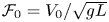 $\mathcal {F}_0=V_0/\sqrt {gL}$, of the fluctuation amplitude
 $\epsilon$ and of the water depth
 $h$.
The hulls are defined by their waterplane, which is vertically extruded in order to form the volume of the hull. The cross-section is an airfoil profile NACA0017 (figure 2d). The motivation for choosing this shape is twofold: the round front enhances wave generation, and the bulk drag coefficients of such profiles are well known and rather low. This allows one to meet conditions where the wave drag is as large as possible with respect to the total drag. In order to vary the Froude number, we change both the velocity and the hull size. The three different hulls are presented in table 1. They have different lengths  $L$ but the same aspect ratios of
 $L/D = 3.6$ and
 $L/B = 6$. The draught is set at
 $T=D/2$ for all the measurements.
Characteristics of the hulls used for the measurements of unsteady resistance ( $L$ is the length,
 $B$ the width and
 $D$ the height).

In order to explore unsteady regimes, we tow the hulls at varying speed  $V(t)$. This sinusoidal speed is set once the mean velocity is reached, which is achieved with a constant-acceleration ramp. For a given hull, this sets the Froude number evolution as
 $\mathcal {F}(t)=\mathcal {F}_0(1 + \epsilon \sin (2{\rm \pi} f t))$. Our experiments are conducted varying the values of
 $\mathcal {F}_0$,
 $f$ and
 $\epsilon$.
The resistance is studied for two values of the mean Froude number, namely  $\mathcal {F}_0 = 0.3$ and
 $\mathcal {F}_0 = 0.57$, which correspond to very different situations for the steady wave drag, as shown in § 3.1. The amplitude
 $\epsilon$ is varied between 0 % (constant speed) and 30 %. The range of tested frequencies goes from
 $0.4$ to
 $3$ Hz. The lower limit is imposed by the finite size of our tank, while the higher limit comes from the maximum acceleration sustained by the set-up.
2.1. The steady velocity limit
A force signal obtained for a steady velocity test is shown in figure 3, towing hull A at  $\mathcal {F}_0 = 0.3$. The data are filtered using a Butterworth lowpass filter of order 6, cutting at 10 Hz. The first and final humps at
 $t=4$ s and
 $t=11.8$ s respectively correspond to the acceleration and deceleration of the hull, while the central part is the total drag force at constant speed. The magnitude of the total resistance is extracted from the difference between the value of the force ‘plateau’ and the value at rest, at the beginning of the recording. The total drag force measured on the hull can be written in the following form:
 \begin{equation} R_{{tot}} = R_{s+f} + R_w + R_I, \end{equation}
where  $R_{s+f}$ refers to the skin and form drag in bulk flow,
 $R_w$ is the wave resistance and
 $R_I$ accounts for the inertial effects.
Example of steady motion force recording for hull A towed at  $V_0 = 0.664\, {\rm m}\,{\rm s}^{-1}$ (
 $\mathcal {F}_0 = 0.3$). The orange time window (P2) is avoided when computing the mean in order to minimize the influence of the initial acceleration (more details in Appendix A).

One can then compute the magnitude of  $R_w$ as
 $R_{tot} - R_{s+f} - R_I$. Here
 $R_I$ is zero during the constant-speed regime and
 $R_{s+f}$ is measured on our hulls using a wind tunnel (see Appendix B for details), so that we can compare the skin and form drag contribution to the wave contribution in the total drag. This comparison is done in § 3.1.
2.2. Unsteady velocity
An example of force signal from unsteady velocity tests is shown in figure 4, towing hull A at  $V_0 = 0.664\, {\rm m}\,{\rm s}^{-1}$ (i.e.
 $\mathcal {F}_0 = 0.3$) with
 $f = 0.8$ Hz and
 $\epsilon = 25\,\%$. Inertial effects are now involved, and dominate when the fluctuation frequency is increased. The magnitude of the total resistance is extracted from the difference between the sensor value over a whole number of periods and its value at rest. This period-wise average enables to eliminate the inertial effects. We also compute the moving average over a whole number
 $N$ of periods:
 $\left \langle R_{tot}\right \rangle _N(t) = ({1}/{NT_0})\int _{t}^{t + NT_0}R_{tot}(\tau )\,{\rm d}\tau$, where
 $T_{0}=1/f$. This quantity evolves towards a constant value, which validates that our measurements correspond to a reliable permanent regime. Details of this verification can be found in Appendix A.
Example of a captured force signal filtered at 10 Hz, towing hull A at  $f=0.8$ Hz,
 $\mathcal {F}_0 = 0.3$,
 $h=25$ cm. The computed mean force is
 $0.34$ N in that case. The orange time window is avoided when computing the mean in order to minimize the influence of the initial acceleration (more details in Appendix A).

For each data point, the measurements are repeated at least three times and the point we plot is the average of the measurements. The error bar is taken as the standard deviation of the repeated measurements for a point, divided by  $\sqrt {n}$, where
 $n$ is the number of repetitions.
3. Experimental results
3.1. Steady-state resistance
The experimental drag coefficient of a hull of immersed volume  $\mathcal {V}=\gamma LTB$ is taken as
 \begin{equation} C_{D{,st}}^{tot} =2\frac{R_{tot,st}}{\rho \mathcal{V}^{2/3}V_0^2}, \end{equation}
with  $R_{tot,st}$ the total drag measured on the hull at constant speed
 $V_0$:
 $R_{tot,st}=R_{s+f{,st}}+R_{w{,st}}$. Parameter
 $\gamma$ has no dimension and depends on the geometry of the hull; in our case
 $\gamma = 0.68$. We plot
 $C_{D{,st}}^{tot}$ for each hull in figure 5(a).
Experimental steady-speed drag coefficients versus the Froude number  $\mathcal {F}_0$. (a) Total drag coefficient
 $C_{D{,st}}^{tot} = 2({R_{tot,st}}/{\rho \mathcal {V}^{2/3}V_0^2})$. (b) Wave drag coefficient
 $C_{w,{st}}=2 (({R_{tot,st} - R_{s+f,st}})/{\rho \mathcal {V}^{2/3}V_0^2})$.

For hulls B and C, the evolution of the total drag coefficient with the Froude number exhibits the typical hump of the wave resistance at  $\mathcal {F}_0 = 0.6$. This shows that the wave resistance is a major part of the measured force. Due to its length, hull A cannot be towed at
 $\mathcal {F}_0>0.6$, but has the same behaviour for the available range of Froude numbers. Wind tunnel measurements of
 $R_{s+f,st}$ (Appendix B) allow one to isolate more precisely the wave drag contribution in the total drag coefficient of figure 5(a). The wave drag coefficient is defined as
 \begin{equation} C_{w,{st}} =2 \frac{R_{tot,st} - R_{s+f,st}}{\rho\mathcal{V}^{2/3}V_0^2}. \end{equation}
The evolution of  $C_{w,{st}}$ is shown in figure 5(b). The details of the calculation of the skin drag
 $R_{s+f,st}$ are given in Appendix B. Figure 5 shows that the wave drag is dominant when the experiment is run close to
 $\mathcal {F}_0=0.6$.
The collapse of curves near  $\mathcal {F}_0 = 0.3$ underlines that depth effects (which should shift the hump position, and its amplitude) are not relevant even for the longer hulls A and B. This is confirmed by computing the value of
 $\tanh {(kh)}$, which appears in the relation of dispersion of pure gravity waves in a fixed frame of reference:
 \begin{equation} \omega^2 = gk\tanh{(kh)}. \end{equation}
For infinitely deep water,  $\tanh {(kh)}$ is asymptotically equal to 1. Taking
 $k=g/V_0^2$, this term is equal to 0.9996 for hull C (
 $V_0=0.76\,{\rm m}\,{\rm s}^{-1}$), and even closer to 1 for hull B (
 $V_0=0.52\,{\rm m}\,{\rm s}^{-1}$) and hull A (
 $V_0=0.66\,{\rm m}\,{\rm s}^{-1}$). This underlines that our experiments belong to the infinite-depth limit.
3.2. Unsteady motion
In this section we present the mean total resistance of a hull following an unsteady motion of the form  $V(t) = V_0 (1+\epsilon \sin (2{\rm \pi} f t))$. We start by varying
 $f$ for a constant
 $\mathcal {F}_0$, and we study the behaviour of the average of the force
 $R_{tot}$ over
 $N$ periods, denoted
 $\left \langle R_{tot}\right \rangle (t) = ({1}/{NT})\int _t^{t+NT}R_{tot}(\tau )\,{\rm d}\tau$, with
 $N$ depending on the characteristics of the hull motion
 $V_0$ and
 $f$.
3.2.1. Evolution of  $\left \langle R_{tot}\right \rangle$ with $f$


With  $\mathcal {F}_0 = 0.3$, and
 $\epsilon = 0.1$, we vary the frequency of the unsteady motion. The evolution of the resistance is shown in figure 6(a) for hull A. Similarly to Doctors et al. (Reference Doctors, Day and Clelland2010), we observe the presence of a hump of resistance for low-frequency oscillation (
 $f<1$ Hz). The peak in hull resistance is found at
 $f=0.7$ Hz and reaches
 $1.1$ times the steady motion value (
 $R_{tot,st}=0.275$ N obtained for
 $\epsilon =0$), then decays slowly while staying above
 $R_{tot,st}$.
Mean total resistance of the hull for unsteady motions. (a) Hull A at  $\mathcal {F}(t) = 0.3 ( 1+ ({1}/{10})\sin (2{\rm \pi} f t))$,
 $R_{tot,st} = 0.276$ N. (b) Hull C at
 $\mathcal {F}(t) = 0.57 ( 1+ ({1}/{10})\sin (2{\rm \pi} f t))$,
 $R_{tot,st} = 0.168$ N. Each red circle is the average over
 $n\geq 3$ measurements at a given
 $f$. The error bars show the associated standard deviation divided by
 $\sqrt {n}$. The blue line ‘QS’ is the quasi-static value of the wave resistance for the unsteady motion. It is obtained with (4.1). The black dashed line ‘st’ shows the steady motion resistance, i.e. when
 $\epsilon = 0$.

For  $f > 2$ Hz, there is roughly no more evolution of the force with the frequency. The quasi-static (QS) estimation (detailed in § 4.1) provides a rough estimate of the order of magnitude of the effect.
Fixing  $\mathcal {F}_0=0.57$, which is a Froude number near the peak of our steady-state resistance curve (figure 5), and varying
 $f$ identically, gives the results presented in figure 6(b). Interestingly, the hump is now going down by
 $4\,\%$ of the steady motion value, and we observe a reduction of the total drag for
 $f<1$ Hz. The effect decays rapidly as
 $f$ is increased, and
 $\left \langle R_{tot}\right \rangle$ seems to become much less sensitive to
 $f$ for
 $f>1$ Hz.
3.2.2. Evolution of $\left \langle R_{tot}\right \rangle$ with $\epsilon$


The effect of the velocity fluctuation amplitude  $\epsilon$ is shown in figure 7 for motions at
 $\mathcal {F}_0 = 0.3$ and
 $\mathcal {F}_0 = 0.57$. It is clear that a larger fluctuation amplitude corresponds to a higher hump amplitude. The resistance for
 $f>1$ Hz though, does not seem to be as much affected by the magnitude of the fluctuation, and for
 $f>2$ Hz, the curves obtained for different
 $\epsilon$ gather within a few per cent away from the steady value.
Mean force on a hull normalized by the constant-speed drag as a function of the fluctuation frequency, for different amplitudes  $\epsilon$. Two Froude numbers are tested. In red: hull A,
 $\mathcal {F}_0 = 0.3$,
 $R_{tot,st} = 0.275$ N. The amplitude is varied from
 $\epsilon = 10\,\%$ to
 $\epsilon = 30\,\%$ by increments of
 $5\,\%$. In blue: hull C,
 $\mathcal {F}_0 = 0.57$,
 $R_{tot,st} = 0.162$ N. The amplitude is varied from
 $\epsilon = 10\,\%$ to
 $\epsilon = 30\,\%$ by increments of
 $10\,\%$.

The sign change of the unsteady effect is further quantified: for a given  $\epsilon$ at
 $\mathcal {F}_0=0.3$, the unsteadiness increases the drag, while it reduces it at
 $\mathcal {F}_0 = 0.57$. The drag change is three times larger in magnitude when
 $\mathcal {F}_0 = 0.3$. In both cases, the unsteady effects measured at large fluctuation (
 $\epsilon = 30\,\%)$ induce a considerable change to the drag when compared with the steady case (
 $+61\,\%$ and
 $-19\,\%$).
In figure 8 we detail the evolution of the mean unsteady resistance as a function of  $\epsilon$, for different values of
 $f$ located in the humps of figure 7. The tendency is well described by a quadratic dependence of the force on the fluctuation amplitude:
 $\left \langle R_{tot}\right \rangle / R_{tot,st} = 1 + \alpha \epsilon ^2$, where
 $\alpha$ is shown to depend on the frequency.
Evolution of the mean drag force normalized by the constant-speed force depending on  $\epsilon ^2$, for different dimensionless fluctuation frequencies
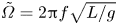 $\tilde {\varOmega }=2{\rm \pi} f\sqrt {L/g}$. This is obtained with hull A at
 $\mathcal {F}_0 = 0.3$ (
 $R_{tot,st}=0.275$ N). The unsteady effect on the drag is a quadratic function of
 $\epsilon$. The slope is larger when
 $f$ is close to the value corresponding to the red peak in figure 7 (roughly
 $0.65$ Hz).

4. Discussion: the quasi-static approach
4.1. Importance of $f$

Trying to understand the effect of the oscillation, we first estimate the QS value of the total drag for the different Froude numbers  $\mathcal {F}_0$. We compute it from the measured values of
 $C_{D{,st}}^{tot}$ in our constant-speed measurements:
 \begin{equation} R_{QS}^{tot} = f \frac{1}{2}\rho LD V_0^2 \int_{0}^{1/f} C_{D{,st}}^{tot}(V(t))(1+\epsilon\sin(2{\rm \pi} f t))^2\,{\rm d}t, \end{equation}
with  $V(t) = V_0(1+\epsilon \sin (2{\rm \pi} f t)$. The graph of
 $C_{D{,st}}^{tot}(V_0) V_0^2$ versus
 $\mathcal {F}_0$ is shown in figure 9 in order to get a better grasp of the result of this integral for hull C. As
 $V(t)$ changes, the Froude number oscillates in the corresponding interval. The resulting evolution of the integrand in (4.1) is shown by the arrows in the zoomed-in plot, where
 $T_{0}=1/f$ is the period of the motion. Starting from
 $\mathcal {F}(t=0) = 0.57$, the system evolves according to arrow 1 until the top speed is reached, then arrow 2, and finally arrow 3 before starting a new period. The larger slope of arrow 3 when compared with arrow 1 makes it clear that the result of the integral (4.1) should be smaller than the resistance for a constant
 $\mathcal {F}_0 = 0.57$. The result for each hull at
 $\epsilon =10\,\%$ is shown by the blue line in figure 6(a,b). This estimation indicates that the average resistance should be higher than the steady state when fluctuating around
 $\mathcal {F}_0 = 0.3$, and lower when
 $\mathcal {F}_0 = 0.57$, which is indeed the behaviour observed experimentally (figure 7).
(a) Evolution of  $C_{D{,st}}^{tot}V_0^2$ versus
 $\mathcal {F}_0$ for hull C at
 $d=0.5$ and
 $h=25$ cm. The central grey area shows the
 $\epsilon =10\,\%$ fluctuation interval around
 $\mathcal {F}_0 = 0.57$. The outer grey area covers the
 $\epsilon =30\,\%$ interval. Additional measurements are made over the fluctuation interval in order to estimate the QS value of the drag. The red lines give an estimate on the slope of the curve on each side of the mean Froude number. (b) A zoomed-in plot focusing on the
 $\mathcal {F}_0 = 0.57 \pm 10\,\%$ interval.

However, the QS description of the unsteady motion comes with an intrinsic caveat when compared with our data: it does not depend on the frequency, which is in contradiction with the experiments (figures 6 and 7). The dependence on the frequency is described quantitatively in the model presented in § 5. Qualitatively, one should expect the QS description to be accurate for vanishingly small values of  $f$. Indeed, the smaller the frequency, the lower the instantaneous acceleration, and the better the QS description. We thus observe that in figure 6, the forces measured at the lowest non-zero values of
 $f$ are in agreement with the QS description. At high frequency, one can see the hull as, essentially, going at steady speed. One way to picture this is to write the distance of the hull to the origin in the frame moving at
 $V_0$. This quantity reads
 $x'(t) = \int _0^t V_0\epsilon \sin (2{\rm \pi} f \tau )\,{\rm d}\tau$: the hull is at its farthest point when at half the period of fluctuation. Hence the length over which the hull is oscillating in that frame is
 \begin{equation} \ell = x'\left(\frac{1}{2f}\right) = \int_0^{1/2f}V_0\epsilon\sin(2{\rm \pi} f \tau)\,{\rm d}\tau = \frac{V_0 \epsilon}{{\rm \pi} f}. \end{equation}
This distance goes to zero for large  $f$: the hull is asymptotically not moving at all in the frame moving at
 $V_0$. This is consistent with our observations in the high end of our frequency interval, where the mean force decays towards the value measured for a constant speed.
4.2. Experimental takeaways
Our study demonstrates that a fluctuating velocity impacts the total drag of an object moving at the water surface, and that the effect can be an increase or a decrease depending on the mean Froude number. In particular, we report drag reduction up to  $-20\,\%$ of the total drag. It occurs near a specific frequency of oscillation, which depends on the Froude number. The amplitude of the fluctuation is a determinant factor in the magnitude of the drag modification.
The effect of varying the velocity should also have an impact on the flow developing underwater, around the hull. Based on the results presented in Appendix B, it seems that the variational drag stems prominently from the wave contribution. This question has received little attention in the past even though it has already been reported that acceleration does have an effect on the viscous drag (Day et al. Reference Day, Campbell, Clelland, Doctors and Cichowicz2011). We thus assumed that such effects, if they exist, were not perturbing our measurements.
5. Theoretical model
The model is based on the theory developed by Havelock (Reference Havelock1928), considering a pressure distribution moving at the interface between air and water. This approach makes it possible to directly isolate the wave drag contribution and to keep the calculation quasi-analytical. It recovers the main features of the wave drag and unsteady effects reported elsewhere (Grue & Palm Reference Grue and Palm1985; Liu & Yue Reference Liu and Yue1993; Palm & Grue Reference Palm and Grue1999).
5.1. Unsteady wave drag
To perturb the water surface we use a Lorentzian pressure distribution:
 \begin{equation} P(\boldsymbol{r})=\frac{P_0b^3}{(b^2 + \left\lVert \boldsymbol{r} \right\rVert^2)^{3/2}}, \end{equation}
with  $P_0$ the pressure in the centre of the distribution,
 $\boldsymbol {r}$ the distance to the centre in the horizontal plane and
 $2b$ the diameter of the distribution. We thus obtain (see Appendix C) the commonly used expression of the wave resistance in Havelock's model (Raphaël & de Gennes Reference Raphaël and de Gennes1996; Gierczak-Galle et al. Reference Gierczak-Galle, Fadle, Arutkin, Raphaël and Benzaquen2020):
 \begin{align} \boldsymbol{R}_w(t) ={-}\displaystyle\int_{0}^t \,\mathrm{d}\tau \displaystyle\int_{0}^{\infty} \,\mathrm{d}k \frac{k^3P_0^2 b^4}{2{\rm \pi} \rho \omega} {\rm e}^{{-}2bk} \sin \left[\omega \left(k\right) \left(t-\tau\right)\right] {\rm J}_1\left[k \left\{r_0\left(t\right)-r_0\left(\tau\right)\right\}\right] \boldsymbol{e}_x, \end{align}
where  $\mathrm {J}_1$ denotes the Bessel function of the first kind of order one. Here the disturbance is moving along the
 $x$ axis following a trajectory
 $r_0(t)$ and
 $k$ is the Fourier space parameter such that
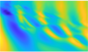
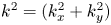 $k^2 = (k_x^2+k_y^2)$. From now on we consider a pulsating velocity around a mean velocity
 $V_0$ :
 \begin{equation} V(t) = V_0 \left(1+\epsilon \sin\varOmega t \right), \end{equation}
where  $\epsilon$ is the amplitude of the velocity pulsation and
 $\varOmega = 2{\rm \pi} f$ the angular frequency of pulsation. In order to define a wave drag coefficient
 $C_w$, we need to define a characteristic velocity and surface. Here, we choose the mean velocity
 $V_0$ as the characteristic velocity. One can then compare the steady velocity case (
 $\epsilon =0$) with pulsating cases using solely the drag coefficient. For the characteristic surface, following the work of Boucher et al. (Reference Boucher, Labbé, Clanet and Benzaquen2018), we define a characteristic volume
 $\mathcal {V}$ using the equilibrium of the pressure disturbance with the gravity field:
 \begin{equation} \rho g \mathcal{V} = \displaystyle\int_0^\infty 2{\rm \pi} P(r)r \,\mathrm{d}r. \end{equation}
The instantaneous wave drag coefficient for an oscillatory motion is then
 \begin{align} C_w(\tilde{t}) &= \dfrac{R_w}{\rho \mathcal{V}^{2/3} V_0^2}\nonumber\\ &= \displaystyle\int_0^\infty \,\mathrm{d} K \frac{K^{5/2} {\rm e}^{{-}K}}{\beta^{4/3} \mathcal{F}_0^2}\nonumber\\ &\quad \times \displaystyle\int_0^{\tilde{t}} \,\mathrm{d}U \sin(\sqrt{K} U ) \mathrm{J}_1 \left[K\mathcal{F}_0 \left\{ U+ \frac{2 \epsilon}{\tilde{\varOmega}} \sin\tilde{\varOmega}\left(\tilde{t}-\dfrac{U}{2}\right)\sin\frac{\tilde{\varOmega}U}{2} \right\}\right], \end{align}
where  $L=2b$ and
 $\sqrt {L/g}$ are used as a characteristic length and time,
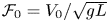 $\mathcal {F}_0=V_0/\sqrt {gL}$ is the Froude number,
 $K = 2bk$ is a non-dimensional wavenumber,
 $\tilde {t}=t\sqrt {g/L}$ is the non-dimensional time,
 $\tilde {\varOmega }= \varOmega \sqrt {L/g}$ is the non-dimensional pulsation and
 $\beta$ is a length over draught aspect ratio arbitrarily defined as
 \begin{equation} \beta = (2{\rm \pi})^{5/4} \frac{ 4\rho g \ell}{P_0}. \end{equation}
Equation (5.5) can be integrated numerically once  $\epsilon$,
 $\mathcal {F}_0$ and
 $\tilde {\varOmega }$ are given. However, as
 $\tilde {t}$ appears in the Bessel function, it is rapidly tedious to compute. In the next sections, we consider some assumptions to simplify the computations.
5.2. Steady velocity ($\epsilon =0$)

In this section, we first consider the simple case of constant velocity  $V(t) = V_0$, or
 $\epsilon =0$. Equation (5.5) can be written in the form
 \begin{equation} C_{w{,st}}(\tilde{t}) = \displaystyle\int_0^\infty \,\mathrm{d} K \frac{K^{5/2} {\rm e}^{{-}K}}{\beta^{4/3} \mathcal{F}_0^2} \displaystyle\int_0^{\tilde{t}} \,\mathrm{d}U \sin(\sqrt{K} U ) \mathrm{J}_1 \left[K\mathcal{F}_0 U\right], \end{equation}
where the subscript  $st$ stands for steady. We display the evolution of
 $C_{w{,st}}$ with time for an impulse start in figure 10(a). The wave drag coefficient oscillates and converges towards a constant value. The period of the oscillations can be measured for different Froude numbers. The natural frequency is
 $\tilde {\varOmega }_r = 1/4\mathcal {F}_0$ as shown in figure 10(b), and is called the Wehausen frequency (Lin et al. Reference Lin, Paulling and Wehausen1964; Liu & Yue Reference Liu and Yue1993), also defined by
 $\tau _r = 2{\rm \pi} f_r V_0/g = 1/4$ (with our notations,
 $\tau _r = \tilde {\varOmega }_r\mathcal {F}_0$).
Steady velocity wave drag coefficient. (a) Time evolution of the wave drag coefficient for an impulse start with  $\mathcal {F}_0 = \mathcal {F}_{0,max}$ defined in (c). (b) Natural frequency of oscillation observed in the impulse start fitted to
 $\tilde {\varOmega }_r=1/4\mathcal {F}_0$. (c) Asymptotic value of the wave drag coefficient.

The asymptotic value of the wave drag coefficient can be evaluated by letting  $\tilde {t}$ go to infinity in (5.7) and it becomes
 \begin{equation} C_{w{,st}}^\infty \left(\mathcal{F}_0 \right)= C_{w{,st}}(\tilde{t}\rightarrow\infty) =\frac{1}{\beta^{4/3}\mathcal{F}_0^8} \int_1^\infty \frac{\xi^{3/2} {\rm e}^{-\xi/\mathcal{F}_0^2}}{\sqrt{\xi-1}} \,\mathrm{d}\xi. \end{equation}
Figure 10(c) shows the evolution of the wave drag with the Froude number. This shape is typical of wave drag coefficient evolution with Froude number (Chapman Reference Chapman1972; Tuck Reference Tuck1989).
5.3. Quasi-static approach
Following our first discussion (§ 4), we start by accounting for the velocity fluctuations with a QS approach. This means that we neglect the time of propagation of the waves compared to the characteristic time of velocity fluctuations ( $\tilde {\varOmega }\ll 1$). The wave drag is then computed as
 \begin{equation} F_{w{,QS}}(t) = \frac{1}{2}\rho \mathcal{V}^{2/3} C^\infty_{w{,st}}\left(\mathcal{F}(t)\right) V_0^2 \left(1+\epsilon \sin \varOmega t\right)^2, \end{equation}
where  $\mathcal {F}(t) = \mathcal {F}_0(1+\epsilon \sin \varOmega t)$ is the instantaneous Froude number. Using the present definition of the instantaneous wave drag coefficient (see (5.5)), we define the QS wave drag coefficient:
 \begin{equation} C^\infty_{w{,QS}} (\tilde{t}) = C_{w{,st}}^\infty\left(\mathcal{F}(\tilde{t}) \right) (1+\epsilon \sin \tilde{\varOmega} \tilde{t})^2. \end{equation}
Assuming  $\epsilon \ll 1$, we can expand the expression and write
 \begin{equation} C^\infty_{w{,QS}} (\tilde{t}) \approx C^\infty_{w{,st}} \left(\mathcal{F}_0\right)+A_{0{,QS}}\left(\mathcal{F}_0\right) \epsilon^2 +A_{1{,QS}}\left(\mathcal{F}_0\right) \epsilon \sin \tilde{\varOmega}\tilde{t}, \end{equation}
where  $A_{0{,QS}}(\mathcal {F}_0) \epsilon ^2$ and
 $A_{1{,QS}}(\mathcal {F}_0) \epsilon$ respectively stand for a correction to the mean wave drag coefficient and the amplitude of oscillation of the wave drag coefficient. The term in
 $2\tilde {\varOmega }$ is neglected here as we choose to keep only the first non-zero corrections to the mean drag and power coefficients. Though
 $A_0$ is a second-order term, it is the first correction to the mean value. The expressions of
 $A_0$ and
 $A_1$ are given in Appendix D.
The shapes of  $A_{0{,QS}}$ and
 $A_{1\textrm {,QS}}$ are displayed in figure 11. We use the maximum wave drag coefficient value
 $\max [C_{w{,st}}^\infty ]$ to re-scale the curves, and denote
 $\bar {A} = A/\max [C_{w{,st}}^\infty ]$ in figure 12 and in the rest of the document. It is worth noting that near the Froude number of maximum wave drag coefficient (
 $\mathcal {F}_{0,max}$; see figure 10c),
 $\overline {A_{0{,QS}}}$ becomes negative. The velocity fluctuations thus lead to a reduction of the mean drag. If we consider a velocity fluctuation of
 $\epsilon =10\,\%$, figure 11 gives the relative correction in percentage terms. The maximum reduction is
 $-2.5\,\%$ near
 $\mathcal {F}_{0,max}$. This estimation is in good agreement with the experimental observations of § 3 (
 $-2.4\,\%$ difference between the ‘QS’ and ‘st’ values in figure 6b).
The QS approach: evolution of the mean (black) and amplitude (blue) of the drag coefficient correction term with the Froude number. Note that with a velocity fluctuation  $\epsilon =10\,\%$, the figure gives the percentage of correction to mean drag coefficient compared with the maximum wave drag coefficient. In both cases,
 $\overline {A_i}=A_i/\max [C_{w{,st}}^\infty ]$.

Evolution of the wave drag coefficient with velocity fluctuations for  $\mathcal {F}_0 = \mathcal {F}_{0,max}$ and
 $\tilde {\varOmega } = 3$. (a) Wave drag coefficient time evolution after an impulse start with
 $\epsilon =0$ (in black) or steady velocity and
 $\epsilon =10\,\%$ (in blue). (b) Difference from the steady case. The blue curve represents the difference between the two curves of (a). The red curve shows the asymptotic regime with the QS approach.

For the amplitude, it appears in figure 11 that the force fluctuations are in phase with the velocity fluctuations for  $\mathcal {F}_0<0.67$. Above this value, the force fluctuations are in opposite phase with the velocity fluctuations. This means that the vessel experiences a minimum wave drag resistance at the maximum velocity.
5.4. General case
In order to describe the effects of the frequency, we relax the QS assumption and look at the actual wave coefficient using (5.5). In figure 12(a), we display the instantaneous drag coefficient of the pulsating case with  $\epsilon =0.1$,
 $\tilde {\varOmega } = 3$ and
 $\mathcal {F}_0 = \mathcal {F}_{0,max}$ and compare it with the steady case (
 $\epsilon =0$). The velocity pulsations lead to fluctuations of the wave drag coefficient around the steady case value. To further outline the impact of the velocity fluctuations on the wave drag coefficient, we subtract from the case
 $\epsilon =0.1$ the instantaneous solution for the steady case and compare it with the previous QS approach. This is shown in figure 12(b). Clear differences appear between the exact solution and the QS approach after a transitional regime. The amplitude of the wave drag coefficient oscillations appears to be largely overestimated in the QS approach and the two curves (blue and red in figure 12b) are out of phase.
To go further, we now expand (5.5) assuming  $\epsilon \ll 1$. Keeping only the first non-zero corrections, it becomes
 \begin{equation} C_w(\tilde{t}) \approx C_{w{,st}}(\tilde{t}) + I_{2}(\tilde{t}) \epsilon^2 + \mathcal{R}\{-\imath {\rm e}^{\imath \tilde{\varOmega} \tilde{t}} I_{1}(\tilde{t})\} \epsilon, \end{equation}
where  $\mathcal {R}$ denotes the real part and
 $$\begin{align} I_1\left(\tilde{t}\right) &= \displaystyle\int_{0}^{\tilde{t}} \,\mathrm{d}U \displaystyle\int_{0}^{\infty} \,\mathrm{d}K \frac{K^{5/2}{\rm e}^{{-}K}}{2\beta^{4/3}\mathcal{F}_0^2 \tilde{\varOmega} U} [ {\rm e}^{-\imath \sqrt{K}U} -{\rm e}^{\imath \sqrt{K}U}+ {\rm e}^{\imath (\sqrt{K}-\tilde{\varOmega} ) U}\nonumber\\ &\quad-\exp({-\imath (\sqrt{K}+\tilde{\varOmega} ) U}) ]\times \left( \mathrm{J}_1 \left[K\mathcal{F}_0 U\right]-K\mathcal{F}_0 U \mathrm{J}_2 \left[K\mathcal{F}_0 U\right] \right) \end{align}$$
and
 $$\begin{align} I_{2}\left(\tilde{t}\right) &= \displaystyle\int_{0}^{\tilde{t}} \,\mathrm{d}U \displaystyle\int_{0}^{\infty} \,\mathrm{d}K \frac{K^{7/2}{\rm e}^{{-}K}}{\beta^{4/3}\mathcal{F}_0 \tilde{\varOmega}^2 U} \sin (\sqrt{K}U) \sin^2\frac{\tilde{\varOmega}U}{2}\nonumber\\ &\quad \times \left( \mathrm{J}_2 \left[K\mathcal{F}_0 U\right]-K\mathcal{F}_0 U \mathrm{J}_1 \left[K\mathcal{F}_0 U\right] \right). \end{align}$$
These two expressions reach an asymptotic regime letting  $\tilde {t}$ go to infinity in the integral term. Past the transitional regime observed in figure 12, we write
 \begin{equation} \left\langle C_w^\infty\right\rangle \approx C_{w{,st}}^\infty\left(\mathcal{F}_0\right) + A_0(\mathcal{F}_0,\tilde{\varOmega}) \epsilon^2. \end{equation}
The expression of  $A_0$ is detailed in Appendix E.
5.5. Phase diagram for the unsteady wave drag
The evolution of the normalized mean drag change due to unsteadiness  $\overline {A_0}$ is depicted in figure 13. The typical values of
 $\tilde {\varOmega }$ and
 $\mathcal {F}_0$ in sports and for some animals are also shown with markers in figure 13. For all the reported values, the points are above the natural frequency
 $\tilde {\varOmega }_r$ (dotted curve on the graph) observed in the impulse start with steady velocity (see figure 10).
Mean wave drag correction as a function of  $\mathcal {F}_0$ and
 $\tilde {\varOmega }$: the colourmap shows the evolution of
 $\overline {A_0}$ in two dimensions. There is a resonance at
 $\tilde {\varOmega } = \tilde {\varOmega }_r = {1}/{4\mathcal {F}_0}$, the Wehausen frequency, marked with the black dotted line. The red curve is plotted in the right-hand panel for a constant
 $\mathcal {F}_0 = \mathcal {F}_{0,max}$ as a function of
 $\tilde {\varOmega }$. The blue (green) horizontal line is plotted in the bottom panel as a function of
 $\mathcal {F}_0$ for
 $\tilde {\varOmega }=4$ (
 $\tilde \varOmega =0.5$). When
 $\tilde {\varOmega }\rightarrow 0$, the curve tends towards the QS approach. The points show typical values of
 $\tilde {\varOmega }$ and
 $\mathcal {F}_0$.

One notices that for a fixed Froude number near the Froude number of maximum wave drag coefficient ( $\mathcal {F}_{0,max}$), the mean drag correction is negative and tends to zero as
 $\tilde {\varOmega }$ increases. This is consistent with the idea that the wave field needs a significant time to settle, and as the frequency of oscillation increases the waves do not have enough time to transport information and momentum to infinity. Hence the wave field does not adapt significantly over a period of oscillation.
Using the QS approach to estimate the mean propulsive force for a known mean velocity can lead to significant errors. For the sake of the discussion we consider the case of a single-scull rowing boat of length  $\ell =2b=8.1$ m and cruising at a mean velocity of
 $V_0=5.1\, {\rm m}\,{\rm s}^{-1}$ (mean velocity for an Olympic race). The typical paddle rate is 31 cycles per minute and the velocity fluctuations are of the order of
 $\epsilon =20\,\%$. The wave drag accounts for approximately 8 % of the total drag of the boat. These values lead to
 $\mathcal {F}_0=0.57$ and
 $\tilde \varOmega =2.9$. This is close to the vertical red line in figure 13. The QS approach will give a reduction of the mean wave drag
 $\overline {A_0}\epsilon ^2 = -10\,\%$. If we use the value derived with our method for the simplified boat, the actual reduction is
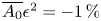 $\overline {A_0}\epsilon ^2 = -1\,\%$. In this example it would be better not to consider the velocity fluctuations for the evaluation of the mean velocity using the mean force or mean power.
We now compare these theoretical predictions with the experiments of § 3.
6. Comparison with experiments and interpretation
6.1. Comparison between experiments and theory
We put our experimental and modelling results next to each other in figure 14. The two values of the average Froude number  $\mathcal {F}_0$ that were investigated experimentally are 0.3 and 0.57. For both of them, the fluctuation frequency was varied, at fixed amplitude
 $\epsilon$. This means that the measured evolutions are described by moving vertically in the parameter space of figure 13: one vertical path at fixed
 $\mathcal {F}_0 = 0.3$, the other at
 $\mathcal {F}_0 = 0.57$. The predicted value of
 $\overline {A_0}$ along those paths is compared with our data in figure 14. In this figure, the wave drag component was isolated using the data from Appendix B. Then the definition of
 $\overline {A_0}$ from the previous section was used to compute its experimental value.
Comparison between our experiments and model predictions for unsteady motions at (a)  $\mathcal {F}_0 = 0.3$ (hull A, circles; hull B, diamonds) and (b)
 $\mathcal {F}_0 = 0.57$ (hull C). The dimensionless coefficient
 $\overline {A_0} = (\left \langle C_w \right \rangle (\tilde {\varOmega })-C_{w,st})/{\max (C_{w,st})\epsilon ^2}$ is plotted against the reduced frequency
 $\tilde {\varOmega }$.

Overall, we observe in figure 14 a good qualitative agreement: the sign and the order of magnitude of the resistance change are consistent between theory and experiments. Again, the model only considers a pressure distribution and thus it is unlikely to lead to quantitative agreement with data from measurements. A better agreement could probably be reached from a refined theory such as that of Lunde (Reference Lunde1951), with, however, the penalty of not having analytical expressions such as the ones presented in Appendix E.
The data points from hull A present the nicest collapse when plotted as a function of  $\overline {A_0}$, because the size of this hull allowed the measured forces to largely overcome the parasitic noise captured by the sensor.
It is clear that for each hull, the experiments at  $\epsilon = 10\,\%$ are quite deviant from the rest of the data. This originates from the fact that at such amplitudes, the drag difference with the steady case is smaller, down to near our measurement resolution.
6.2. Geosimilar rescaling
The hulls used for our experiments are geometrically similar. Hence, provided that finite-depth and finite-width effects are negligible, and that the skin friction is subtracted adequately, the dimensionless wave resistance curves are expected to collapse on a single curve for identical dimensionless test conditions, i.e. same values of  $\mathcal {F}_0$,
 $\tilde {\varOmega }$ and
 $\epsilon$. Our data allow us to test this for hulls A and B, both travelling at
 $\mathcal {F}_0 = 0.3$, for two different fluctuations. The result shown in figure 15 is a very good agreement between the data series. This shows that the wave drag coefficient of geometrically similar vessels is indeed identical, and that applying a three-dimensional scaling factor
 $\alpha$ to the hull dimensions multiplies the wave drag by
 $\alpha ^{2}$.
Mean wave drag coefficient  $\left \langle C_w \right \rangle = \left \langle R_w \right \rangle /(0.5\rho \mathcal {V}^{2/3}V_0^2)$ as a function of the fluctuation frequency, at
 $\mathcal {F}_0 = 0.3$. Hulls A and B differ by a geometric three-dimensional scaling factor of 5/3.

6.3. Interpretation
There are several length scales in our problem: the most immediate ones are the boat length  $L$ and the wavelength
 $\lambda$ of the generated waves. Starting back from the dispersion relation in deep water
 $\omega ^2 = gk$, and considering waves for which the phase speed
 $c_\varphi = \omega /k$ is equal to
 $V_0$, one gets that
 \begin{equation} \lambda = 2{\rm \pi} V_0^2/g = 2{\rm \pi} L \mathcal{F}_0^2. \end{equation}
The ratio between  $L$ and
 $\lambda$ is connected to the Froude number, which is a known feature of steady wave drag.
The unsteadiness introduces a new length scale. It corresponds to the shortest distance between two locations where the hull is moving at a same speed, during its sinusoidal speed variation. We call it  $\varLambda$ and upon integrating
 $V(t)$ over one period, one gets
 \begin{equation} \varLambda = V_0/f. \end{equation}
These lengths  $\lambda$ and
 $\varLambda$ can be compared to understand that a resonance is happening when the frequency of the velocity variation is tuned correctly (or poorly). Doing so, we have that
 \begin{equation} \frac{\lambda}{\varLambda} = \frac{2{\rm \pi} L \mathcal{F}_0^2}{V_0/f} = \tilde{\varOmega}\mathcal{F}_0. \end{equation}
If we replot the data of figure 7 using this quantity for the  $x$ axis, we get the graph shown in figure 16. The
 $y$ axis has been changed to display the non-dimensional drag modification due to unsteadiness, normalized by
 $\epsilon ^2$:
 $({\left \langle R_{tot}\right \rangle - R_{tot,st}})/{R_{tot,st}\epsilon ^2}$. The
 $\epsilon = 10\,\%$ series aside, all the experiments at fixed
 $\mathcal {F}_0$ boil down to an identical behaviour. The obvious difference with the previous choice of
 $x$ coordinate is that both humps are now found at the same location on the axis. This observation supports the hypothesis of a resonance, which would happen at a given value of
 $\lambda /\varLambda$, denoted
 $\mathcal {F}_0\tilde {\varOmega }_r$.
Unsteady contribution to the wave drag normalized by  $\epsilon ^2$, for different amplitudes
 $\epsilon$. Water depth is 25 cm, and two Froude numbers are tested. Positive values: hull A,
 $\mathcal {F}_0 = 0.3$. The amplitude is varied from
 $\epsilon =10\,\%$ (light red) to
 $\epsilon =30\,\%$ (dark red) by increments of
 $5\,\%$. Negative values: hull C,
 $\mathcal {F}_0=0.57$. The amplitude is varied from
 $\epsilon = 10\,\%$ (light blue) to
 $\epsilon = 30\,\%$ (blue) by increments of
 $10\,\%$.

For our experiments, in the case  $\mathcal {F}_0 = 0.3$ we obtain maximum unsteady wave drag
 $\left \langle R_{tot}\right \rangle (\tilde {\varOmega }) - R_{tot,st}$ for
 $0.85 \leq \tilde {\varOmega } \leq 0.99$, which corresponds to
 $\lambda /\varLambda$ between 0.25 and 0.3 (the green dashed line in figure 16 stands at
 $\lambda /\varLambda =0.28$). In other words, experimentally we have that
 $\widetilde {\varOmega _r} \propto 1/\mathcal {F}_0$ with a factor of around 0.28. This dependency is recovered by our model, with a factor of 0.25, as shown in figure 10(b). This value was also obtained experimentally by Cleaver et al. (Reference Cleaver, Calderon, Wang and Gursul2013). As a comparison, Doctors et al. (Reference Doctors, Day and Clelland2010) obtain a value of
 $\mathcal {F}_0 \tilde {\varOmega }_r$, that they denote
 $\tau$, between 0.23 and 0.24 for the peak resistance in a similar situation. They are working with a 3 m long Wigley hull, in a 75.8 m long towing tank. These experimental results are consistent with our model. The difference in the exact value of the parameter is likely to come from experimental uncertainty associated with the discretization of the frequency axis (typically three points to resolve the peak). This is also consistent with theoretical predictions showing that a singularity occurs when the parameter
 $\tau = \mathcal {F}_0 \tilde {\varOmega }=V_0 2{\rm \pi} f/g$ reaches the value of 1/4 (Grue & Palm Reference Grue and Palm1985; Liu & Yue Reference Liu and Yue1993; Palm & Grue Reference Palm and Grue1999).
The effect can also be explained with the Wehausen frequency. The resonance is found to happen precisely when  $\tilde {\varOmega }$ is close or equal to the Wehausen frequency
 $\tilde {\varOmega }_r$, which corresponds to natural oscillations of the wave resistance after the system changes speed. Since in our case the speed is constantly changing, this frequency is present in the system at all times. When the system starts fluctuating at this same frequency, a resonance takes place that amplifies the drag modification.
As for the change of the unsteady effect (being either an increase or a decrease of the total drag), it seems to be contained in the QS description. When fluctuating around the peak of the  $C_w(\mathcal {F}_0)$ curve (figure 10c), the resistance is smaller on average, as shown in figure 9. The opposite effect takes place around
 $\mathcal {F}_0 = 0.3$. The work of Grue & Palm (Reference Grue and Palm1985) explains the possible appearance of drag reduction through the existence of a wave carrying negative energy away from the vessel.
7. Conclusion
Our experiments investigated unsteady motion resistance under various conditions. Placed in a context where the wave drag was the most largely varying force, total drag force measurements were performed on hulls moving at  $V(t) = V_0(1 + \epsilon \sin (2{\rm \pi} f t))$. The study is in line with previous works on that problem (e.g. Grue & Palm Reference Grue and Palm1985; Doctors et al. Reference Doctors, Day and Clelland2010) and new experimental results, as well as theoretical drag coefficients, are presented.
It was shown that the periodic velocity fluctuation has a different impact on the average drag depending on the value of the Froude number 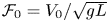 $\mathcal {F}_0=V_0/\sqrt {gL}$. At
 $\mathcal {F}_0 = 0.3$, the average drag can be increased by the velocity fluctuations, up to a dramatic amount (near 60 %) when
 $\epsilon$ is large (typically 30 %). At
 $\mathcal {F}_0 = 0.57$, the average drag can be reduced by the speed fluctuations, by up to 19 % when
 $\epsilon = 30\,\%$. These effects were found maximal in a frequency range around
 $\tilde {\varOmega } = 2{\rm \pi} f\sqrt {L/g} \sim 0.65$ in the former case and
 $\tilde {\varOmega } \sim 0.6$ in the latter. In both cases, the effect of unsteadiness on the average drag becomes negligible for values of
 $\tilde {\varOmega }$ above
 $2.5$. At given values of
 $\tilde {\varOmega }$ and
 $\mathcal {F}_0$, the average drag modification from unsteadiness was shown to be proportional to
 $\epsilon ^2$, the square of the velocity fluctuation amplitude. The proposed understanding was the appearance of a resonance when the ratio of the wavelength of the waves to that of the fluctuating motion reaches a theoretical value of
 $1/4$, measured to be around 0.28 here. Equivalently, this was when the forcing of the speed fluctuation
 $\tilde {\varOmega }$ gets close to the natural frequency of oscillation of the wave resistance in steady motion after an impulse start, known as the Wehausen frequency
 $\tilde {\varOmega }_r$.
A theoretical description of the simplified problem based on an extension to Havelock's theory was proposed. Considering a Lorentzian pressure distribution moving at sinusoidal speed at the surface of water, we obtained a phase diagram in ( $\mathcal {F}_0$,
 $\tilde {\varOmega }$) for the average drag coefficient modification due to the unsteadiness of the motion. The predictions of this model compared qualitatively well with the experimental data, and the diagram allows one to assess the importance of velocity fluctuations regarding the wave drag for a given motion.
Concerning the application of the study to unsteady motion in sports, and especially for rowing boats, our results showed that for a sinusoidal speed (taken as a first-order approximation of the actual speed in rowing), there is no significant unsteady effect on the wave drag at the values of  $\mathcal {F}_0\tilde {\varOmega }$ encountered in races. The case of swimmers (smaller
 $\tilde {\varOmega }$, closer to the region with unsteady effects) might actually be more interesting as a situation where unsteady effects should be considered for optimizing performance.
Acknowledgements
The authors are grateful to M. Benzaquen, M. Ferrand, F. Picella, M. Rabaud and G. Rousseaux for useful discussions. They also thank the Fablab of Ecole Polytechnique, and especially G. Paterson, who has been a great help with the technical experimental work. Finally, the authors would like to thank R. Labbé and his team from Phyling, who designed and manufactured the force sensor used for the measurements and provided guidance in handling. They acknowledge the support from CNRS for this research.
Funding
The authors thank the National Research Agency (ANR) which contributed to the study via the project THPCA $^{2024}$ dedicated to high-performance cycling and rowing (ANR-2020-STHP2-0006).
Declaration of interests
The authors report no conflict of interest.
Appendix A. Validation of the unsteady measurements
Figure 17 shows the evolution of the moving average in unsteady motion for some frequencies. The curve is either flat by the end of the tank, or decreasingly oscillating around an asymptotic value. In the latter case, the asymptotic force was also estimated by fitting the data. The forces measured this way fall within the error bars of the values we obtained from averaging on a whole number of periods. This is an indication that merely taking this average does not twist the data.
(a) Examples of a moving average on the force signal, towing hull A at different frequencies. The time window for the average is one period of the unsteady motion. The signals are plotted after a 10 Hz filtration. Here  $\mathcal {F}_0 = 0.3$,
 $h=25\,{\rm cm}$. (b) Fitting the
 $f=1.4$ Hz signal of (a) with a form
 $\varGamma (t) = R_w + R_{w{,st}}\cos (\omega (t-t_0)+\varphi )(\omega _\infty (t-t_0))^N$. The free parameters are
 $\omega$,
 $\varphi$ and
 $N$.

Besides, the study of Doctors et al. (Reference Doctors, Day and Clelland2008) allows a better understanding of such oscillations. Following their work, we write that
 \begin{equation} R_w (t) = R_{w,\infty} + R_{w{,st}} \cos(\omega (t-t_0) + \varphi)(2\omega_\infty(t-t_0))^N , \end{equation}
with  $R_{w,\infty }$ the average resistance value,
 $R_{w{,st}}$ the initial magnitude of the moving average fluctuation,
 $\omega$ its pulsation,
 $\omega _\infty = g/4V_0$ the Wehausen frequency and
 $N<0$ a decay exponent. The instant
 $t_0$ corresponds to the end of the initial acceleration ramp, and we perform the fit starting one period after
 $t_0$. This expression is originally applied to the wave resistance of a body reaching a constant speed
 $U$ after an initial fixed acceleration ramp. The analogy with our case is that the moving average should, since our motion is periodic, behave similarly and reach towards a constant. In figure 17 we present two examples of fits for moving averages. The fitted quantities from (A1) are the pulsation
 $\omega$, the phase
 $\varphi$ and the decay exponent
 $N$. We recover values of
 $N$ in the range of those described by Doctors et al. (Reference Doctors, Day and Clelland2008) (
 $N$ between
 $-0.9$ and
 $-0.5$ depending on the initial acceleration, for
 $\mathcal {F}_0 = 0.3$), which supports the idea that these oscillations are not an obstacle to the evaluation of the mean resistance within the extent of the tank. The signal would become constant if the tank was long enough, and the asymptotic value is well-enough estimated by the average over several periods.
For the same reason, the average we make on steady-speed force signals does not start immediately after the initial acceleration.
Appendix B. Skin friction $R_{s+f}$

This appendix presents measurements of the skin and form drag  $R_{s+f}$ in a wind tunnel.
These measurements were made using hulls of the same shape, NACA0017, with fixed length  $L$ and varying height
 $D$ (see figure 18). The values of
 $D$ we used are those of the three hulls A, B and C. We added an extra one of height
 $0.25$ m in order to approach the edgeless case limit. The force
 $R_{s+f}$ is measured with a six-axis sensor, and the model is placed facing the flow at zero angle of attack. The drag force can be written as the sum of two contributions:
 $R_{s+f} = R_{s+f}^{{bulk}} + R_{s+f}^{{edges}}$. The bulk contribution can be estimated with XFoil (Drela Reference Drela1989), which computes the drag coefficient
 $C_D^{{bulk}}$ in a purely two-dimensional case. In other words, the total drag reads
 \begin{equation} \left. \begin{aligned} R_{s+f} & = \frac{1}{2}\rho LDC_D^{{bulk}}(Re_L)V_0^2 + \frac{1}{2}\rho BL(2C_D^{{edge}}(Re_L))V_0^2,\\ R_{s+f} & = \frac{1}{2}\rho LDC_D^{{bulk}}(Re_L)V_0^2 \left(1 + 2\frac{B}{D} \frac{C_D^{{edge}}}{C_D^{bulk}}(Re_L) \right), \end{aligned} \right\} \end{equation}
where  $C_D^{{edge}}$ is the drag coefficient associated with the presence of one edge. For a given hull shape, this coefficient only depends on the Reynolds number
 $Re_L=V_0L/\nu$.
(a,b) Models used for the wind tunnel measurements. Heights  $D_1 = 5$ cm,
 $D_2 = 8.3$ cm,
 $D_3 = 14$ cm,
 $D_4 = 25$ cm. The length and width of the four models are
 $L = 30$ cm and
 $B = 5$ cm.

We start with measuring the coefficient  $C_D^{{bulk}}$ in the wind tunnel. To do so, we subtract the aerodynamic drag of a model of height
 $D_1$ from that of a taller model of height
 $D_2>D_1$. Since the edges are identical for those models, the remaining contribution is that of a virtually edgeless hull of height
 $D^* = D_2-D_1$:
 \begin{equation} R_{s+f}(D^*) = \tfrac{1}{2}\rho LD^* C_D^{bulk}(Re_L)V_0^2. \end{equation}
Thus we can deduce the value of  $C_D^{bulk}(Re_L)$ for the Reynolds numbers in the wind tunnel. This is done with two pairs of hulls
 $(D_2, D_1)$ such that
 $D^*$ is 11 and 17 cm. The experimental bulk coefficients are shown in figure 19. They are expected to be identical because the longitudinal sections of all the models are the same. The theoretical value obtained from XFoil in a purely two-dimensional case is shown in black as a reference. The large differences at low Reynolds numbers result from the sensitivity limit of the sensor.
Bulk drag coefficient of a NACA0017 measured in a wind tunnel. Values computed with XFoil for the ideal two-dimensional (2-D) case are added as a reference.

The mean Reynolds numbers  $Re_L$ for the hulls in the towing tank are:
 $3.3\times 10^5$ for hull A,
 $1.5\times 10^5$ for hull B and
 $1.3\times 10^5$ for hull C. Over this range of
 $Re_L$, the values of the bulk coefficient are plateauing above the ideal value. This is likely to be an effect of the surface roughness, known to increase the minimum drag of symmetrical airfoils (Chakroun, Al-Mesri & Al-Fahad Reference Chakroun, Al-Mesri and Al-Fahad2004). We thus approximate the bulk drag coefficient to a constant
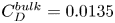 $C_D^{bulk}=0.0135$ in this domain of
 $Re_L$.
We now use (B1) to obtain the value of  $C_D^{edge}$ for each of our wind tunnel models. Again, it should be identical across the models. In figure 20 we plot the ratio
 ${C_D^{{edge}}}/{C_D^{bulk}}(Re_L)$ for the models that relate to the towing tank hulls. For hulls A, B and C we take from figure 20 that
 $({C_D^{{edge}}}/{C_D^{bulk}})(Re_L) = 0.88$ constant (based on the
 $T=8.3$ cm model, which has the same
 $B/D$ as the hulls) in the experimental range of
 $Re_L$.
Edge drag coefficient of a NACA0017 normalized by the bulk drag coefficient, computed from (B1).

Using these results, it is possible to estimate the skin friction drag on the hulls in the towing tank, including the edge effect from the bottom of the strut, using a modified drag coefficient:
 \begin{equation} R_{s+f} = \tfrac{1}{2}\rho LT C_{s+f} V_0^2, \end{equation}
with
 \begin{equation} C_{s+f} = C_D^{bulk}\left(1+\frac{B}{T} \frac{C_D^{edge}}{C_D^{bulk}}\right). \end{equation}
Compared with (B1), the coefficient 2 has disappeared since only one edge is in water, and the draught  $T$ is now the relevant vertical length.
This study allows one to compare  $R_{s+f}$ and
 $R_w$. Doing so, we get that the wave drag is dominant in the towing tank experiments only for hull C (78 % of the total drag). This makes sense since these experiments are run at the peak of the wave drag coefficient curve (see figure 5b). Hulls A and B are towed at
 $\mathcal {F}_0 = 0.3$, which corresponds to a much lower value of
 $C_w$. Hence, despite the chosen hull shape, the wave drag is not dominant at steady speed in those experiments (21 % for hull A, 37 % for hull B).
However, the qualitative predictions of our model still seem to hold for hull A, as can be seen in figure 14. This is believed to come from the much stronger dependency of  $C_w$ on the velocity (through
 $\mathcal {F}_0$) compared with
 $C_{s+f}$ (through
 $Re_L$).
Appendix C. Derivation of the wave resistance in Havelock's model
An external Lorentzian pressure distribution,  $P_{ext}(\boldsymbol {r},t)$, moves on the free surface along the
 $x$ axis with a velocity
 $V(t)$ and generates a wake. The disturbance trajectory is given by
 \begin{equation} \boldsymbol{r}_0(t) = \displaystyle\int_0^t \,\mathrm{d}t'\, V(t') \boldsymbol{e}_x, \end{equation}
and the external pressure is considered undeformable such that
 \begin{equation} P_{ext}\left(\boldsymbol{r},t\right) = P\left(\boldsymbol{r}- \boldsymbol{r}_0(t)\right), \end{equation}
where  $P(\boldsymbol {r})$ is the pressure field located at the initial time at the position
 $\boldsymbol {r}_0 = \boldsymbol {0}$. We call
 $\zeta (\boldsymbol {r},t)$ the displacement of the free surface from its equilibrium position and assume small perturbations. We neglect second-order terms in the fundamental equations. The flow of an ideal, homogeneous, incompressible, infinitely deep fluid with a free surface
 $z = \zeta (x,y,t)$ is then governed by the linearized Euler equations with boundary conditions:
 \begin{equation} \left. \begin{array}{ll@{}} \boldsymbol{\nabla}\boldsymbol{\cdot}\boldsymbol{u} = 0, & z \in \left]-\infty,\zeta\right],\\ \partial_t \boldsymbol{u} +\dfrac{1}{\rho}\boldsymbol{\nabla}p - \boldsymbol{g} = 0, & z \in \left]-\infty,\zeta\right],\\ p = P_{ext}, & z = \zeta,\\ \partial_t \zeta + \boldsymbol{u}_h\boldsymbol{\cdot}\boldsymbol{\nabla}\zeta - w = 0, & z = \zeta,\\ \partial_z\varphi \rightarrow 0, & z\rightarrow - \infty, \end{array} \right\} \end{equation}
where 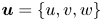 $\boldsymbol {u} = \{u,v,w\}$ is the velocity field,
 $g$ denotes the gravitational acceleration,
 $p$ is the pressure and
 $\boldsymbol {u}_h =\{u,v\}$ is the horizontal velocity at the free surface. Capillary effects are neglected. We further consider the flow irrotational and
 $\boldsymbol {u}=\boldsymbol {\nabla }\varphi$, where
 $\varphi$ is the scalar velocity potential. Injecting in the continuity equation, one has
 \begin{equation} \Delta \varphi=0. \end{equation}
The linearized Bernoulli equation is classically derived using the momentum equation:
 \begin{equation} \partial_t \varphi + \frac{1}{\rho} p + g z = 0, \quad \forall \boldsymbol{x}. \end{equation}
Injecting in the surface boundary conditions, it becomes
 \begin{equation} \partial_{t,t} \varphi + g\partial_z \varphi + \partial_t\left(\frac{P_{ext}}{\rho} \right) =0, \quad\text{at} \ z=0. \end{equation}
The free surface can then be deduced using the Bernoulli equation:
 \begin{equation} \zeta ={-}\frac{1}{g} \left(\partial_t \varphi +\frac{P_{ext}}{\rho} \right). \end{equation}
Keeping in mind the boundary condition at  $z\rightarrow -\infty$ and (C4), we define the two-dimensional Fourier transform
 $\hat \varphi (k_x,k_y)$ of the scalar velocity potential:
 \begin{equation} \varphi\left(x,y,z,t\right) = \displaystyle\int_{\mathbb{R}^2} \,\mathrm{d}k_x\,\mathrm{d}k_y \, \widehat{\varphi} \left(k_x,k_y,t\right) \exp\left({\imath k_x x + {\rm i}k_y y}\right) {\rm e}^{k z}, \end{equation}
where 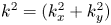 $k^2 = (k_x^2+k_y^2)$. Taking the Fourier transform of (C6), it becomes
 \begin{equation} \left(\partial_{t,t} + g k \right) \hat \varphi ={-}\frac{\hat P}{\rho} \exp\left({\imath \boldsymbol{k}\boldsymbol{\cdot} \boldsymbol{r}_0(t)}\right), \end{equation}
where  $\hat P$ is the Fourier transform of the external disturbance
 $P(\boldsymbol {r})$. Applying the operator
 $(\partial _{t,t} + g k )$ to the Fourier transform of (C7), one can find the equation for the evolution of
 $\hat \zeta$:
 \begin{equation} \partial_{t,t} \hat\zeta + \omega^2 \hat\zeta ={-}k \frac{\hat P}{\rho} \exp\left({\imath \boldsymbol{k}\boldsymbol{\cdot} \boldsymbol{r}_0(t)}\right), \end{equation}
where  $\omega ^2 = gk$ is the dispersion relation in deep water. Assuming no disturbance at
 $t=0$, one gets a general solution for the surface elevation:
 \begin{equation} \hat\zeta\left(k_x,k_y,t\right) ={-}\displaystyle\int_0^t \,\mathrm{d}\tau\, \frac{k \hat P}{\rho \omega} \sin \left[\omega \left(k\right) \left(t-\tau\right)\right] \exp\left({\imath \boldsymbol{k}\boldsymbol{\cdot} \boldsymbol{r}_0(\tau)}\right). \end{equation}
The instantaneous horizontal forces exerted on the surface, called hereafter wave drag, are given by
 \begin{equation} \boldsymbol{R}_w(t) ={-}\displaystyle\int_{\mathbb{R}^2} P_{ext} \boldsymbol{\nabla}\zeta \,\mathrm{d}\kern0.7pt x\,\mathrm{d} y. \end{equation}
Using the properties of the Fourier transform, it becomes
 \begin{equation} \boldsymbol{R}_w(t) = \displaystyle\int_{0}^t \displaystyle\int_{ \mathbb{R}^2} \frac{\imath k \left| \hat P \right|^2 \sin \left[\omega \left(k\right) \left(t-\tau\right)\right] } { 4{\rm \pi}^2\rho \omega \exp\left({\imath \boldsymbol{k}\boldsymbol{\cdot} \left\{\boldsymbol{r}_0(\tau)-\boldsymbol{r}_0(t) \right\}}\right) }\boldsymbol{k}\,\mathrm{d}k_x\,\mathrm{d}k_y\,\mathrm{d}\tau. \end{equation}
This formula is valid for any pressure distribution moving on a surface. We now consider a Lorentzian pressure distribution:
 \begin{equation} P(\boldsymbol{r})=\frac{P_0b^3}{\left(b^2 + \left\lVert \boldsymbol{r} \right\rVert^2\right)^{3/2}}, \end{equation}
where  $P_0$ is the pressure maximum and
 $b$ a characteristic length of the perturbation. The Fourier transform is
 \begin{equation} \hat P(\boldsymbol{k})=P_0 b^2 {\rm e}^{{-}b k }. \end{equation}
Injecting the expression of  $\hat P$ into (C13) and integrating on a circle of radius
 $k$ for a trajectory along the
 $x$ axis,
 $\boldsymbol {r}_0(t) = r_0(t) \boldsymbol {e}_x$, one obtains
 \begin{align} \boldsymbol{R}_w(t) ={-}\displaystyle\int_{0}^t \,\mathrm{d}\tau \displaystyle\int_{0}^{\infty} \,\mathrm{d}k \frac{k^3P_0^2 b^4}{2{\rm \pi} \rho \omega} {\rm e}^{{-}2bk} \sin \left[\omega \left(k\right) \left(t-\tau\right)\right] \mathrm{J}_1\left[k \left\{r_0\left(t\right)-r_0\left(\tau\right)\right\}\right] \boldsymbol{e}_x, \end{align}
which is the exact same equation as (5.2).
Appendix D. Expression of $A_{0{,QS}}$ and $A_{1{,QS}}$


From (5.8) we get the asymptotic value of the wave drag coefficient:
 \begin{equation} C_{w{,st}}^\infty \left(\mathcal{F}_0 \right)= C_{w{,st}}(\tilde{t}\rightarrow\infty) =\frac{1}{\beta^{4/3}\mathcal{F}_0^8} \int_1^\infty \frac{\xi^{3/2} {\rm e}^{-\xi/\mathcal{F}_0^2}}{\sqrt{\xi-1}} \,\mathrm{d}\xi. \end{equation}
This can also be written in the form
 \begin{equation} C_{w{,st}}^\infty \left(\mathcal{F}_0 \right)= \dfrac{{\rm e}^{{-}1/2\mathcal{F}_0^2}}{2\mathcal{F}_0^8\beta^{4/3}}\left\{\mathcal{K}_0\left(\dfrac{1}{2\mathcal{F}_0^2}\right)+\left(1+\mathcal{F}_0^2\right) \mathcal{K}_1\left(\dfrac{1}{2\mathcal{F}_0^2}\right)\right\}, \end{equation}
where  $\mathcal {K}_i$ denotes the Bessel function of the second kind of order
 $i$.
Similarly, the correction coefficients of the wave drag coefficient in the QS limit are
 \begin{align} A_{0{,QS}} \left(\mathcal{F}_0\right) &= \dfrac{{\rm e}^{{-}1/2\mathcal{F}_0^2}}{8\mathcal{F}_0^8\beta^{4/3}}\left\{ \left(4-26\mathcal{F}_0^2 +33 \mathcal{F}_0^4\right)\mathcal{K}_0\left(\dfrac{1}{2\mathcal{F}_0^2}\right) \right. \nonumber\\ &\left. \quad +\left(4-22\mathcal{F}_0^2 +13 \mathcal{F}_0^4+6\mathcal{F}_0^6\right)\mathcal{K}_1\left(\dfrac{1}{2\mathcal{F}_0^2}\right) \right\},\end{align}
 \begin{align} A_{1{,QS}} \left(\mathcal{F}_0\right) &= \dfrac{{\rm e}^{{-}1/2\mathcal{F}_0^2}}{2\mathcal{F}_0^{10}\beta^{4/3}}\left\{ \left(2-5\mathcal{F}_0^2\right)\mathcal{K}_0\left(\dfrac{1}{2\mathcal{F}_0^2}\right) \right. \nonumber\\ &\left.\quad +\left(2-3\mathcal{F}_0^2-2\mathcal{F}_0^4\right)\mathcal{K}_1\left(\dfrac{1}{2\mathcal{F}_0^2}\right) \right\}. \end{align}
Appendix E. Expression of $A_{0}$

The expression of  $A_0$ is given by the limit for infinite time of
 $I_2$. This yields
 $$\begin{gather} A_{0}(\mathcal{F}_0,\tilde\varOmega) = \displaystyle\int_{0}^{\infty} \,\mathrm{d}U \displaystyle\int_{0}^{\infty} \,\mathrm{d}K \frac{K^{7/2}{\rm e}^{{-}K}}{\beta^{4/3}\mathcal{F}_0 \tilde{\varOmega}^2 U} \sin (\sqrt{K}U) \sin^2\frac{\tilde{\varOmega}U}{2}\nonumber\\ \times \left( \mathrm{J}_2 \left[K\mathcal{F}_0 U\right]-K\mathcal{F}_0 U \mathrm{J}_1 \left[K\mathcal{F}_0 U\right] \right). \end{gather}$$
Expanding the product, we can write
 \begin{equation} A_{0}(\mathcal{F}_0,\tilde\varOmega) = {\rm J}_{1,+}+{\rm J}_{1,-}-{\rm J}_2, \end{equation}
where
 $$\begin{gather} {\rm J}_{1,\pm} = \dfrac{1}{4\mathcal{F}_0^3\beta^{4/3}\tilde{\varOmega}^2}\displaystyle\int_0^{\infty} \,\mathrm{d}K \dfrac{K^{3/2} {\rm e}^{{-}K} (\sqrt{K} \pm \tilde{\varOmega})^3}{\sqrt{(\mathcal{F}_0K)^2 - (\sqrt{K}\pm \tilde{\varOmega})^2}}\varTheta[ (\mathcal{F}_0K)^2 - (\sqrt{K}\pm \tilde{\varOmega})^2], \end{gather}$$
 $$\begin{gather}{\rm J}_2 = \dfrac{1}{2\mathcal{F}_0^3 \beta^{4/3}\tilde{\varOmega}^2} \displaystyle\int_0^{\infty} \,\mathrm{d}K \dfrac{K^{5/2} {\rm e}^{{-}K}}{\sqrt{\mathcal{F}_0^2K -1}}\varTheta(\mathcal{F}_0^2 K-1), \end{gather}$$
where  $\varTheta$ is the Heaviside function.


 Open access

