Introduction
In conservation paleobiology, it has become common practice to use death assemblages to reconstruct recent historical communities and environments (e.g., Goodfriend Reference Goodfriend1992; Noble et al. Reference Noble, Curran and Wilson1995; Greenstein and Pandolfi Reference Greenstein and Pandolfi1997; Brewster-Wingard and Ishman Reference Brewster-Wingard and Ishman1999; Kowalewski et al. Reference Kowalewski, Serrano, Flessa and Goodfriend2000; Burney et al. Reference Burney, James, Burney, Olson, Kikuchi, Wagner, Burney, McCloskey, Kikuchi and Grady2001; Edinger et al. Reference Edinger, Pandolfi and Kelley2001; Espinosa et al. Reference Espinosa, De Francesco and Isla2003; Edgar and Samson Reference Edgar and Samson2004; Frenzel and Boomer Reference Frenzel and Boomer2005; Ferguson and Miller Reference Ferguson and Miller2007; Ferguson Reference Ferguson2008; Simões et al. Reference Simões, Rodrigues and Kowalewski2009; Terry Reference Terry2010; Erthal et al. Reference Erthal, Kotzian and Simões2011; Miller Reference Miller2011; Yanes Reference Yanes2012; Roff et al. Reference Roff, Clark, Reymond, Zhao, Feng, McCook, Done and Pandolfi2013). Opportunities to assess changing community composition through recent time intervals are especially valuable because they have the potential to provide direct, kinetic information about biological responses to environmental change. To track compositional changes through time, serial records of life and death assemblages are desirable. In general, however, sequential live census data that span multiple decades are not available for life or death assemblages in most shallow-marine settings (but see Holland Reference Holland1985; Nichols Reference Nichols1985; Edmunds Reference Edmunds2002; Feser and Miller Reference Feser and Miller2014).
Because the upper several tens of centimeters of sediment in shallow-marine environments are typically subjected to intense mixing by callianassid shrimp and other bioturbators, the original age order of sediments and constituent death assemblages tends to be partially or entirely obscured, thereby limiting their usefulness either in or for assessment of temporal changes in community composition (Suchanek Reference Suchanek1983; Kowalewski et al Reference Kowalewski, Goodfriend and Flessa1998; Kosnik et al. Reference Kosnik, Hua, Kaufman and Wüst2009; Tomašových and Kidwell Reference Tomašových and Kidwell2010). The dense root–rhizome mats that characterize Thalassia-rich seagrass beds, however, may provide an opportunity to overcome this limitation by: (1) significantly inhibiting bioturbation (Peterson Reference Peterson1982) and (2) stabilizing sediments against physical disturbance (Widdows et al. Reference Widdows, Pope, Brinsley, Asmus and Asmus2008).
Here, we test the hypothesis that dense seagrass beds sampled around St. Croix, USVI, yield more stratigraphically intact, less thoroughly time-averaged molluscan death assemblages than have been reported in other shallow-marine substrates (e.g., Parsons-Hubbard et al. Reference Parsons-Hubbard, Hubbard, Tems and Burkett2014). To assess this, we extracted sediments in discrete sedimentary intervals in quantities sufficient to generate statistically robust samples of the local molluscan biota. While a similar method has recently been used by Kosnik et al. (Reference Kosnik, Kaufman and Hua2013) and Parsons-Hubbard et al. (Reference Parsons-Hubbard, Hubbard, Tems and Burkett2014), the former sampling was conducted primarily in sand-covered substrates, and the latter used smaller-bore cores, resulting in shallow samples with orders-of-magnitude fewer skeletal elements. Thus, this is the first case that we are aware of in which larger, stratigraphically sequential samples were extracted from dense seagrass substrates with the goal of testing for downward compositional stratigraphy.
Second, we hypothesize that if constituent death assemblages have not been stratigraphically homogenized, compositional changes up to and including the present can be diagnosed statistically and that shallower death assemblages are more similar to their associated life assemblages than are deeper death assemblages.
Setting and Field Methods
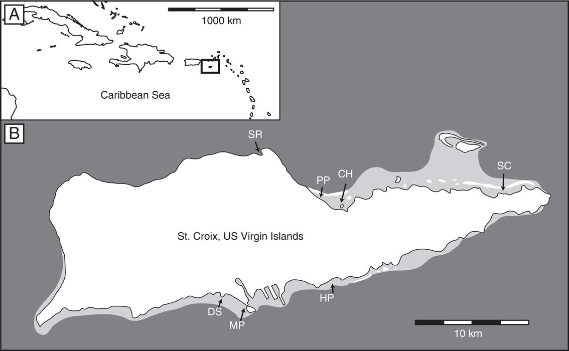
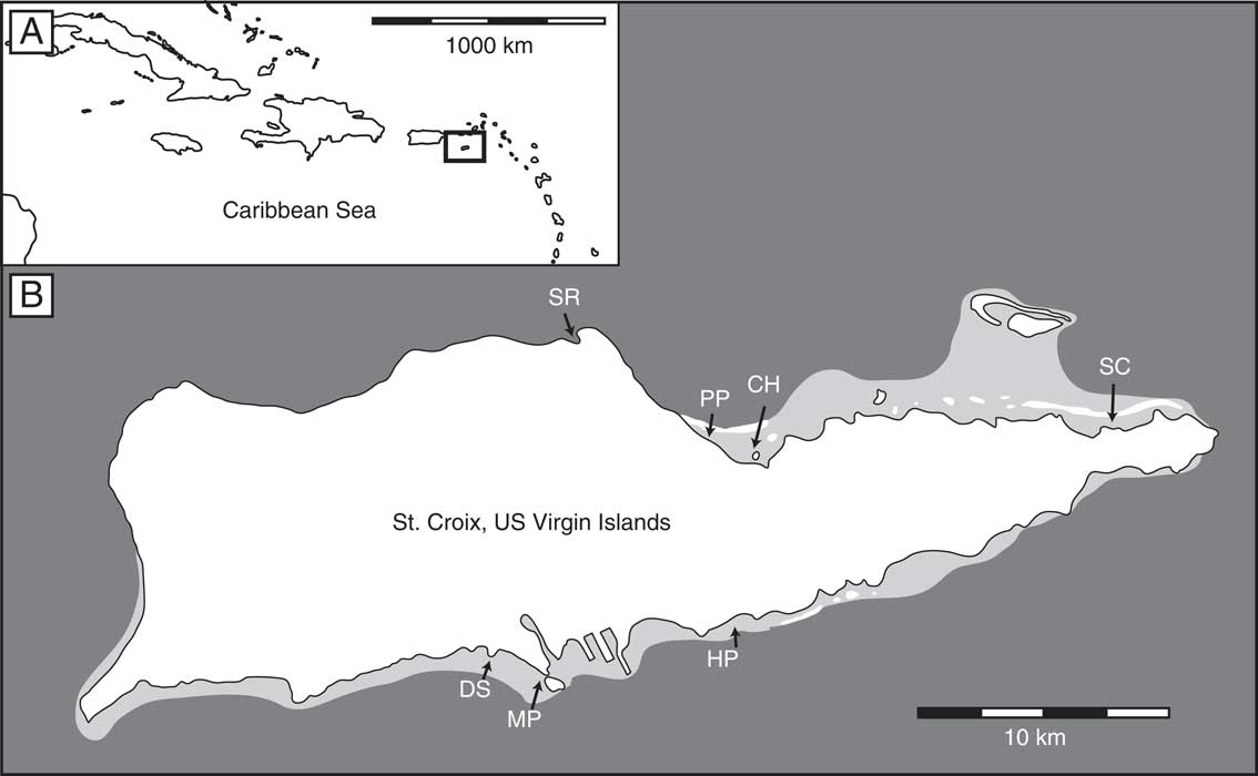
The island of St. Croix is located on an insular platform southeast of Puerto Rico at the northern end of the Lesser Antilles (Fig. 1A). In areas where the shelf extends several hundred meters or more offshore, notably along the northeast and southern coastlines, extensive seagrass beds are present. We targeted seven localities where substrates were dominated by dense seagrass during two collecting seasons: one in June 2011 and another in December 2012 (Fig. 1B). Because the present study was part of a larger investigation of potential anthropogenic changes to local biotas and environments, we chose localities based on their proximity to specific anthropogenic agents. We sampled four Thalassia-rich localities on the north shore: the relatively less developed Smuggler’s Cove (SC), an area adjacent to a tourist resort in Christiansted Harbor (CH), the island’s power plant (PP), and the estuary and recreational boat marina located in Salt River Bay (SR). We sampled three additional localities along the south shore near the island’s primary municipal dump, which extends into the sea as an artificial peninsula (DS), the former HOVENSA oil refinery/oil storage facility and nearby Martin Marietta aluminum refinery near Molasses Pier (MP), and up-current from MP at the relatively less developed Ha’Penny Bay (HP).
Map of the seven localities sampled around St. Croix, USVI. Medium gray fill indicates the extent of the carbonate shelf, while dark gray is off the platform (B). (A) Inset map indicates St. Croix’s position in the Caribbean Sea. SC, Smuggler’s Cove; CH, Christiansted Harbor; DS, dump site; HP, Ha’Penny Bay; MP, Molasses Pier; PP, power plant; SR, Salt River Bay.
At each locality, we positioned sampling transects within the area of densest, laterally contiguous seagrass, avoiding as much as possible the margins of the bed. Seagrass beds were generally dominated by the wide-bladed species, Thalassia testudinum, with lesser abundances of the thinner-bladed Syringodium filiforme and Halodule wrightii, although Syringodium surpassed Thalassia in terms of raw abundance at some localities (see “Results” section). A variety of macroalgae were also present, including species of Halimeda, Penicillus, and Caulerpa. To quantify the density of vegetation, seagrass and macroalgae were censused by haphazardly dropping a 10 × 20 cm quadrat onto the seafloor near each sample station and recording the abundances of all species present (blades of seagrass or clumps of macroalgae). This process was repeated four to six times at each station.
At most localities, we established 30 m transects and sampled them every 10 m, for a total of four stations per transect. At some localities, including PP and CH, only two of the four stations were sampled each year. Only one station was sampled at DS in 2011, but based on a preliminary analysis of the contents of the initial sample, we sampled a longer, 90 m transect, oriented perpendicular to shore, to investigate possible compositional gradients moving away from the artificial peninsula.
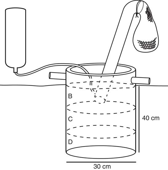
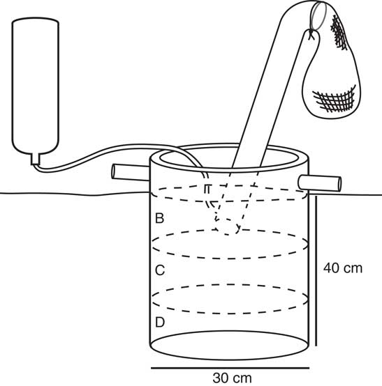
Each station was sampled using a custom-designed, cylindrical 30 cm diameter by 50 cm tall steel coring template. With the aid of a saw blade built into its base, we manually sank the template 40 cm into the substrate at each station. We then airlifted the contents in three separate depth samples of ~13 cm and sieved each through a 2 mm mesh bag attached in situ (Fig. 2); in the “Results” and “Discussion” sections, the sample closest to the sediment–water interface is designated as the “B” sample, the stratigraphically intermediate sample is designated as the “C” sample, and the deepest sample is designated as the “D” sample. Back on shore, samples were preprocessed for removal of plant material and some clearly extraneous, non-molluscan sediment, and were then stored in 70% alcohol to preserve soft materials of molluscan individuals that were alive at the time of sampling.
Schematic diagram of the sampling apparatus, including dimensions. Letters B, C, and D represent the shallowest, middle, and deepest sedimentary intervals, respectively. The airlift, constructed from PVC, had a 2 mm mesh bag attached to the outflow end, and the compressed-air tank provided lift.
In the lab, we sieved the samples again, discarding any material less than 2 mm and then manually picked mollusks from the remaining sediments. To avoid any possibility of counting multiple fragments of the same individual, and thereby artificially inflating abundances, only gastropods with an intact apex and bivalves with an intact umbo were retained for analyses. Individuals containing soft tissues (i.e., “live” individuals) were separated from dead elements during this process; these are referred to as the “A” sample. Greater than 80% of live individuals were collected from B intervals, and less than 3% were extracted from the D interval. We used standard references (Abbott and Morris Reference Abbott and Morris1995; Redfern Reference Redfern2001; Mikkelsen and Bieler Reference Mikkelsen and Bieler2008) to identify species, and each species’ abundance in a given sample was recorded and used for subsequent numerical analyses.
A limited number of radiocarbon dates were obtained to provide age estimates for death assemblages. Ten valves of the prolific venerid bivalve Chione were selected from all three sedimentary intervals from the 90 m station at DS. These valves were cut in half, sonicated, and sent to the Keck AMS lab at University of California–Irvine for radiocarbon dating.
Analytical Methods
Replicates of all vegetation abundance censuses at each locality were pooled to construct box-and-whisker plots representing median and upper and lower quartiles for each of the six primary macrofloral taxa. Abundances represent raw values in order to facilitate direct comparisons of vegetation density within the 10×20 cm quadrat. All quantitative analyses were conducted in the statistical programming environment, R, Version 3.4.0 (R Core Team 2017).
For analyses of molluscan data, raw abundances were transformed in two ways. First, bivalve abundances were halved to account for the possibility that any given individual could contribute two valves to the death assemblage. Coupled with the inclusion of only bivalve specimens with umbos, this value represents the minimum number of actual bivalve individuals in a given sample, the so-called MNI approach used by numerous previous researchers (Gilinsky and Bennington Reference Gilinsky and Bennington1994; Reitz and Wing Reference Reitz and Wing2008). Although not halved, the restriction of gastropod counts only to specimens with apices also yields MNI estimates. Second, the abundance of each species in a given sample was recast as a percentage of the total abundance of specimens in the sample to mitigate variations in sample size (for the locality-level ordinations, rarefaction was performed first, as described later).
A full-island death assemblage analysis was first conducted to investigate compositional variation among localities around St. Croix: samples were compared with one another using the Bray-Curtis pairwise similarity coefficient, coupled with nonparametric multidimensional scaling (NMDS) using the metaMDS function in R (Bray and Curtis Reference Bray and Curtis1957; Clarke and Warwick Reference Clarke and Warwick2001). Samples were plotted in the first two NMDS dimensions. Both the overarching and locality-specific ordinations included convex hulls; in the former case, hulls circumscribed all samples from a single locality, and in the latter case, they circumscribed all samples from a single sedimentary interval.
To further investigate death assemblage (DA) compositions in relation to life assemblages (LAs), locality-level ordinations were calculated that included both the LAs and DAs. To mitigate for the smaller sample size, and therefore generally greater compositional dispersion of the LAs, we rarefied DAs by resampling without replacement to the size of their corresponding LAs (Tomašových and Kidwell Reference Tomašových and Kidwell2009). This was done using the function rrarefy in R, which is based on Hurlbert’s (Reference Hurlbert1971) formulation. The resulting samples were size standardized to sample totals using the decostand function in the ‘vegan’ package.
Analysis of similarity (ANOSIM) was performed to test for significant differences among groups. The resulting test statistics (R) and their associated significance values (p) are reported within the ordination plots and reflect comparisons among sedimentary interval groups (B, C, D). Additional ANOSIM tests were performed using differently defined groups and are described and reported in the text. R values typically range between 0, indicating no discrimination among groups, and 1, indicating that all samples within a group are more similar to one another than to samples from any other group (Clarke and Warwick Reference Clarke and Warwick2001). If the p-value is significant (<0.05), we can reject the null hypothesis (nondiscrimination).
A similarity percentages (SIMPER) analysis was used to determine which species had the greatest contribution to among-group differences (Clarke Reference Clarke1993). This analysis was applied to each locality separately, and because of the large number of combinations (each sedimentary interval was compared with every other sedimentary interval), species that consistently contributed the most to overall among-interval dissimilarity were reported. For those selected species, the values provided represent the average relative abundances for each of the most meaningful taxa in the A, B, C, and D sedimentary intervals.
Live/dead fidelity (sensu Kidwell and Flessa Reference Kidwell and Flessa1996; Kidwell Reference Kidwell2007) was quantified using both Spearman’s rho, a rank-based correlation metric, and Bray-Curtis similarity, which evaluates the similarity of two samples based on species’ relative abundances (Clark and Warwick Reference Clarke and Warwick2001). Jaccard’s coefficient, a presence/absence metric, was also calculated but is not included here, because it showed an almost linear relationship to rho. Fidelity was calculated individually for each sedimentary interval, resulting in three comparisons for each station (where A = live): A/B, A/C, and A/D. LA and DA samples for a given transect were pooled together prior to calculation of fidelity metrics to produce robust, statistically viable comparisons. The patterns we observe at this resolution are also observable, albeit with greater variability, when transects are separated into their constituent stations.
Results
Among-Locality Spatial Variation
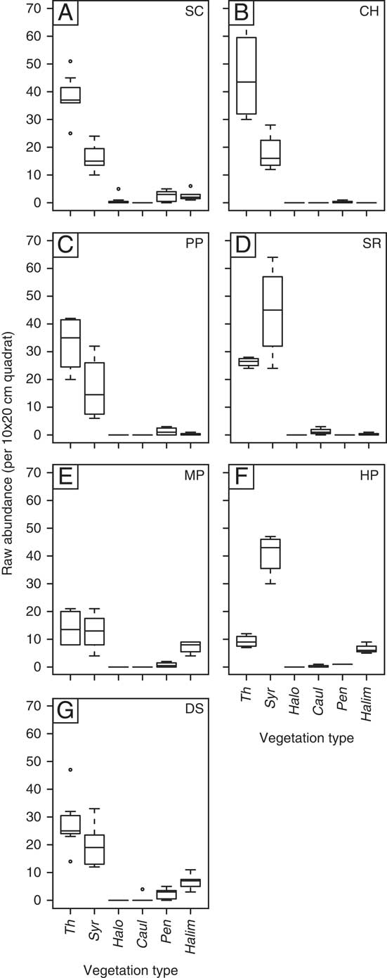
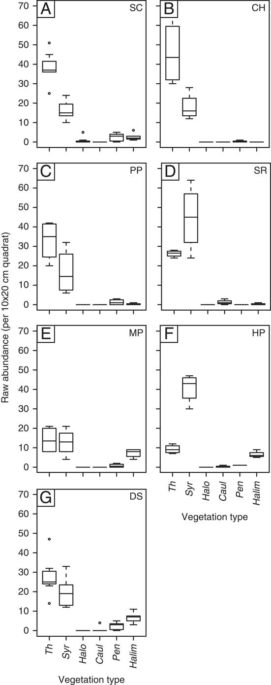
While we made an effort to only sample localities that were characterized by dense, continuous seagrass, there was some variation in the precise abundance and composition of present-day vegetation (Fig. 3). At SC, CH, PP, and DS, median Thalassia testudinum abundances were significantly higher than those of Syringodium filiforme, the second most common taxon. MP had virtually identical contributions from both species, and SR and HP showed a greater abundance of S. filiforme than T. testudinum, although T. testudinum density was quite high, on the order of 27 blades per 10×20 cm quadrat at SR. Furthermore, it must be kept in mind that the surface area provided by a single Thalassia blade is far greater than that of Syringodium (Miller Reference Miller1988), so that actual T. testudinum cover far exceeds that of S. filiforme at every locality except HP. Halimeda sp. was an appreciable contributor primarily at the three southern localities: MP, HP, and DS.
Average raw abundances of seagrass and macroalgae measured using 10 × 20 cm quadrats. Horizontal line within box represents median value, box encompasses upper and lower quartiles, dotted lines (“whiskers”) extend to maximum values, excluding outliers, which are shown as dots. Vegetation abbreviations are as follows: Caul, Caulerpa; Halim, Halimeda; Halo, Halodule; Pen, Penicillus; Syr, Syringodium; Th, Thalassia.
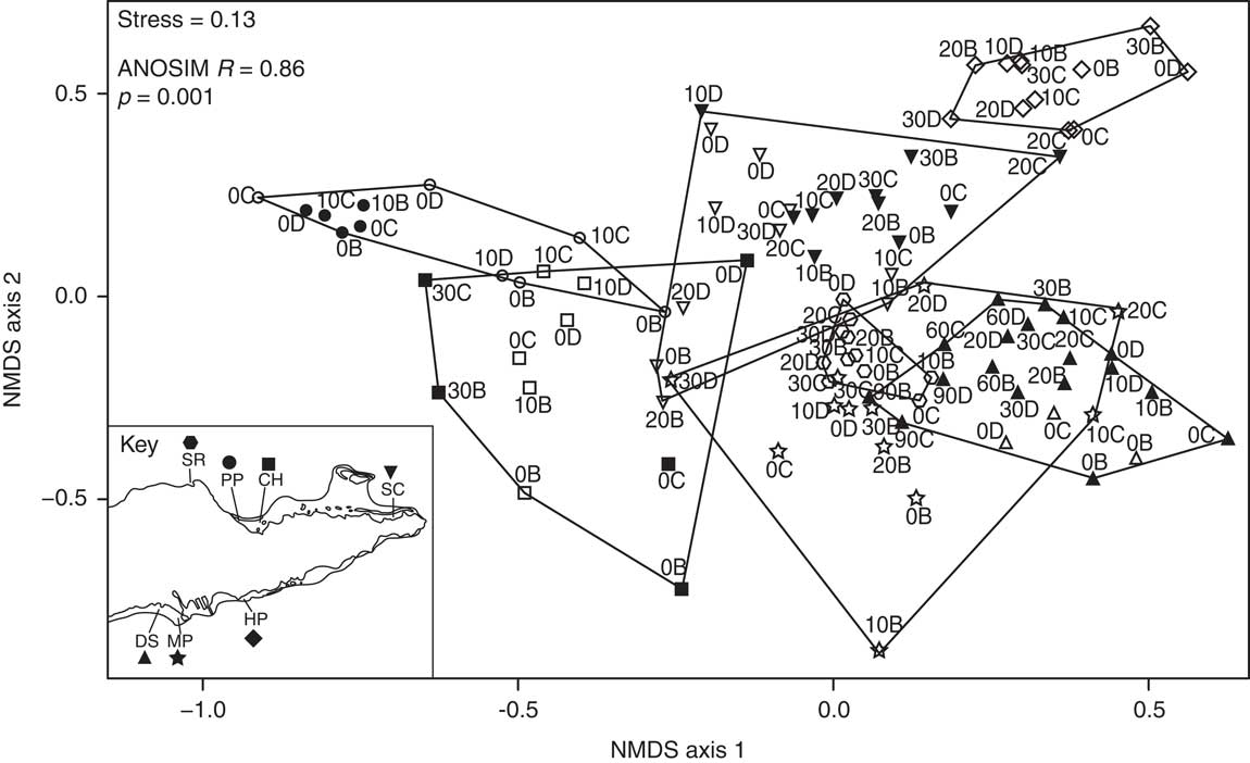
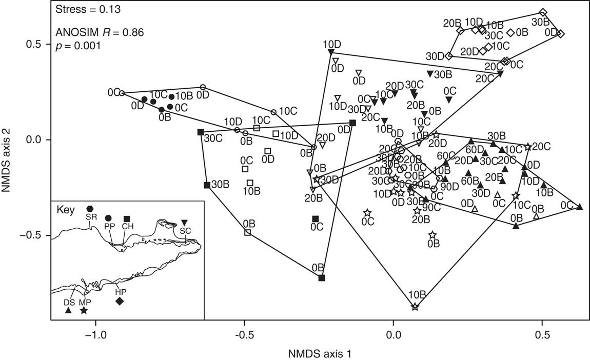
An island-wide comparison of death assemblage composition reveals greater among- than within-locality variation, as evidenced by an ANOSIM R value of 0.86 (p=0.001). This is evidenced as well in the NMDS ordination (Fig. 4), in which the convex hulls circumscribing each locality are largely distinct from one another, and samples from individual localities tend to group in the same region of ordination space.
Ordination of all samples at all localities plotted on NMDS axes 1 and 2. Sample symbols correspond to their localities (see key; abbreviations defined in Fig. 1 legend), and convex hulls encompass all samples for a given locality. ANOSIM R and corresponding p-value reflect the extent (and significance) of compositional differences among the seven localities. Filled symbols represent samples collected in 2012, and open symbols represent samples collected in 2011. Labels reflect each sample’s position on the transect (e.g., 10 m) and sedimentary interval (B, C, or D).
Down-Core Variation in Species Composition
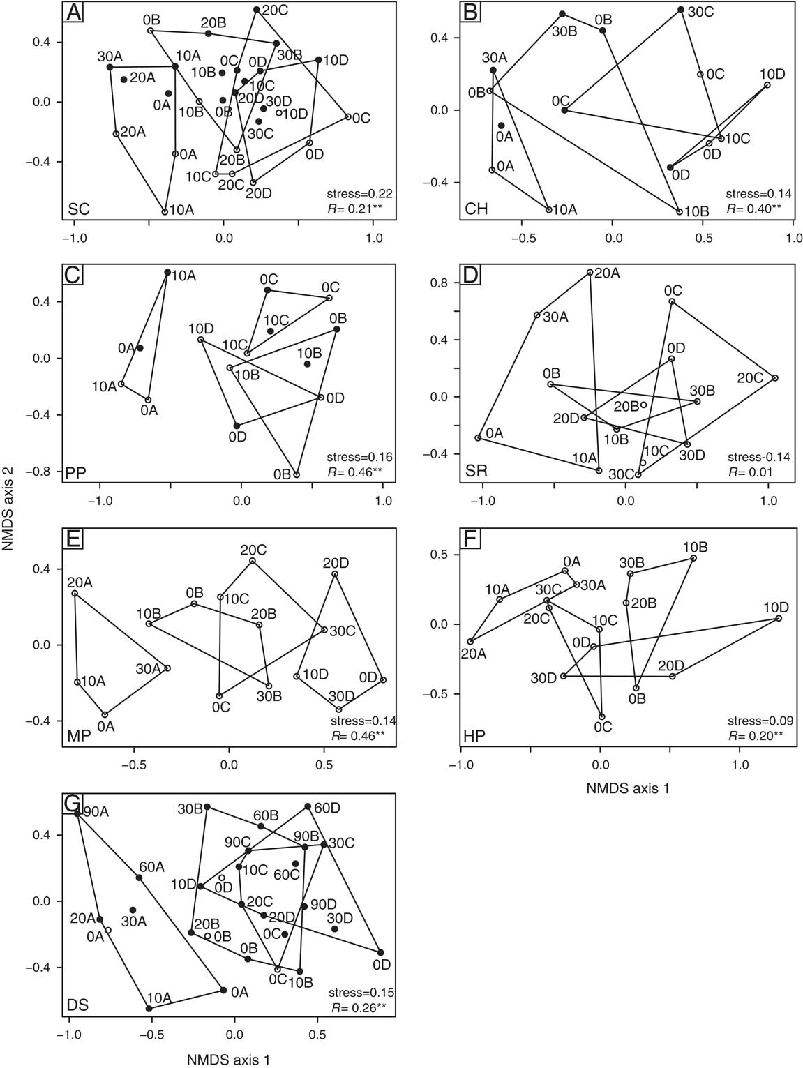
Convex hulls that encompass each sedimentary interval in NMDS ordinations of each locality (Fig. 5) reveal that, while there is overlap among sedimentary intervals at all localities, assemblages are not homogenized down-core, as would be expected in a thoroughly bioturbated substrate, and a distinctive stratigraphy is evident in some cases. ANOSIM R values range from nearly 0 at SR (Fig. 5D) to a maximum of 0.46 at both PP and MP (Fig. 5C,E). With the exception of SR, all other R values are significant, suggesting that sedimentary intervals are grouped to a greater extent than would be expected given a random distribution. This down-core variation is not consistently exhibited along a single NMDS axis, but is in many cases oriented roughly parallel to the first axis. Furthermore, in several instances, notably SC, CH, and MP, variation roughly follows a down-core gradient along the first axis; that is, intervals A, B, C, and D are arrayed in order along the axis (Fig. 5A,B,E). At the remaining localities, down-core variation does not follow the strict “ABCD” order but nevertheless, still tends to convey compositional differences with depth.
Individual NMDS ordinations for each of the seven localities; abbreviations defined in Fig. 1 legend. Live samples are distinguished by the “A” label. Differentiation between 2011 and 2012 samples and labeling scheme are the same as for Figure 4. Convex hulls distinguish samples from A, B, C, and D intervals. All panels compare the first and second NMDS axes.
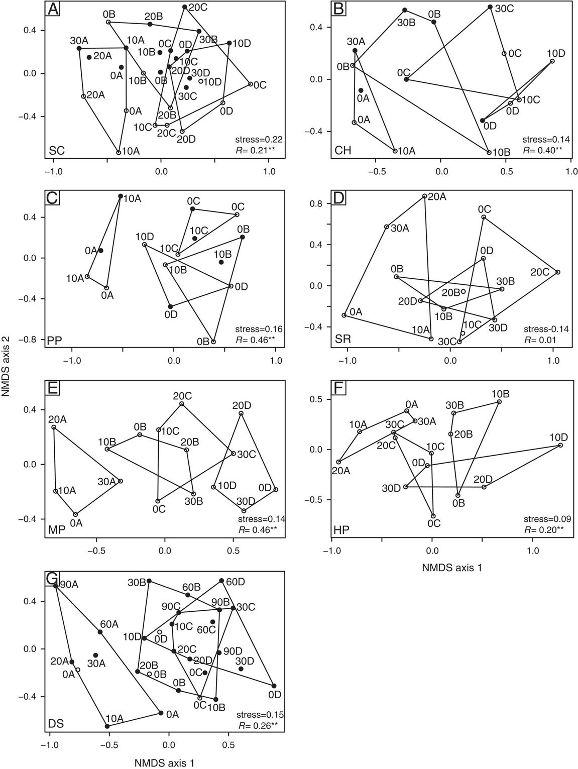
Ordinations reveal a number of patterns that describe the degree of similarity among depth assemblages. First, LA (A) samples are typically compositionally distinct from their associated DAs. In cases where they do overlap (e.g., SC, CH, and SR), it is typically with the shallowest (B) samples (Fig. 5A,B,D). In some cases, the three death assemblages all show high similarity to one another, as evidenced by their three overlapping convex hulls (as at SC and DS). In other cases, two intervals overlap to a considerable degree, and the third remains fairly distinct (as at PP, SR, and MP). A third, less common pattern shows fairly distinct groups within each of the three sedimentary intervals (as at CH). Finally, at the HP locality, B and C are distinct from one another, but both overlap with the D samples. Samples collected in different years show different patterns as well. At SC and CH, there is an indistinct separation of 2011 and 2012 samples on the second axis, but at PP and DS, a similar distinction does not exist (Fig. 5A,B,C,G, respectively).
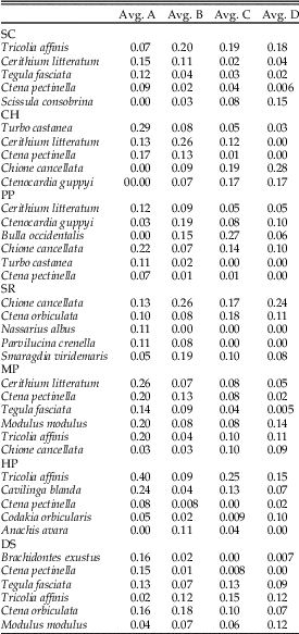
The SIMPER analysis provides more detailed information regarding species that have the greatest contribution to overall dissimilarity down-core but: (1) species that contribute the most to dissimilarity among groups are not the same for all localities; (2) variation in relative abundance of each species is not necessarily monotonic down-core; and (3) because SIMPER only compares two groups, species displayed for each locality have been compiled from multiple comparisons (A to B, A to C, A to D, etc.).
The epifaunal gastropods Tricolia affinis, Cerithium litteratum, Tegula fasciata, Turbo castanea, and Modulus modulus are all identified as important contributors to down-core variation at multiple localities (Table 1). Of these, T. affinis generally increases with depth, while C. litteratum, T. fasciata, and T. castanea generally decrease. While it varies down-core, M. modulus does not exhibit monotonic change within localities. Bulla occidentalis, which contributes to among-interval change at PP, exhibits a maximum relative abundance in the C sample at that locality.
Species identified by the SIMPER analysis as contributing significantly to down-core variation at each locality. Average relative abundances for each species in each sedimentary interval (including live, A) at a given locality are provided as decimals in columns 1–4.

Infaunal bivalves including the lucinids Ctena pectinella, Parvilucina crenella, and Ctena orbiculata, the venerid Chione cancellata, and the cardiid Ctenocardia guppyi are also prominent contributors to down-core variation at multiple localities. Of these, only C. pectinella (decreasing) and C. cancellata (increasing) show systematic down-core variation at multiple localities. Notably, the abundant epifaunal mussel Brachidontes exustus sharply decreases down-core at DS, and the infaunal tellinid Scissula consobrina systematically increases down-core at SC.
Live/Dead Fidelity Down-Core
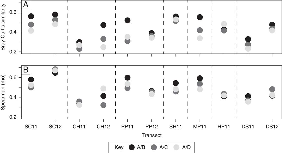
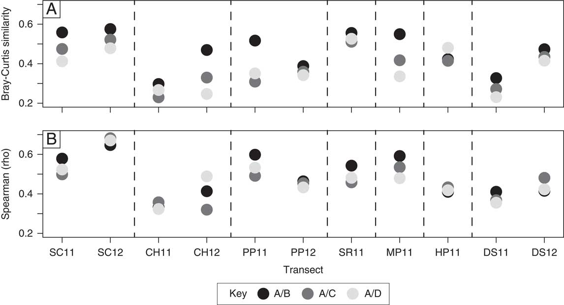
When data from a single transect (i.e., all samples from a single locality in a given year) were pooled, DA fidelity to the LA generally increased as the LA was compared with successively shallower sedimentary intervals (Fig. 6). This pattern was most evident based on the Bray-Curtis similarity coefficient, in which 7 of the 11 transects showed increasing fidelity up-core (Fig. 6A). Of the remaining four transects, three displayed greater A/B than A/D similarity. Only one transect (HP) exhibited higher A/D than A/B fidelity. This pattern was not as apparent for Spearman’s rho values. Only 7 of the 11 transects showed higher A/B than A/D fidelity, and dispersion among calculated values for a given transect was generally lower (Fig. 6B).
Calculations of live/dead fidelity with depth based on Bray-Curtis similarity (A) and Spearman’s rho (B). Samples pooled to transect scale. Dotted lines separate transects from each locality. Year that transect was sampled designated in labels as “11” or “12.”
Establishing Age Constraints
Chronologies established from marine sediment cores indicate that sea level was ~10 m below its current level ~7000 years ago (Kennett Reference Kennett1982; Burke et al. Reference Burke, Adey and MacIntyre1989), and St. Croix’s platform is thought to have flooded around that time (Parsons-Hubbard et al. Reference Parsons-Hubbard, Hubbard, Tems and Burkett2014). The oldest death assemblage shells could not have accumulated before this flooding event, so 7000 years serves as a maximum Holocene shell age. It is very likely, however, that the DAs we sampled are much younger, given that we only penetrated the upper 40 cm of sediment, so estimating sedimentation rates over the last 7000 years allows for a rough calculation of the amount of time represented by each sedimentary interval. Holocene sediment thickness at SC, where it has been measured by other researchers, averages ~2.7 m but the maximum thickness is less than 5 m at all measured SC sites (Parsons-Hubbard et al. Reference Parsons-Hubbard, Hubbard, Tems and Burkett2014). Based on these values, and assuming a simplified steady rate of sedimentation, we estimate a maximum sedimentation rate of ~70 cm/1000 years. The entire thickness of sediment sampled, 40 cm, would then represent a minimum of ~600 years, and each sedimentary interval would represent ~200 years.
Preliminary geochronological analysis using radiocarbon dating of C. cancellata shells from DS have provided us with age estimates for the sedimentary package at that locality. The oldest sampled shells from the D interval provided ages averaging ~1500 cal yr BP. Shells from the B interval yielded ages of ~50 yr BP. Additional analyses will be necessary to determine accurate age ranges for each interval and to establish ages for shells from the C interval.
Discussion
Spatial Variation in Mollusk Composition
The full-island ordination (Fig. 4) suggests a high degree of structure that is partitioned on a variety of spatial and temporal levels. The locality-level groups represented by the hulls in the ordination produce an ANOSIM R value of 0.86, suggesting that samples within localities are more similar to one another than they are to samples from other localities. Because benthic mollusks are sensitive to their substrates, one potential driver of among-locality differences is the minor variation in vegetation cover observed from locality to locality (Fig. 3). In general, localities with higher concentrations of Thalassia have lower axis 1 values, and those with higher Halimeda concentrations have higher axis 1 values. While it might be expected that B intervals, which are closest to the sediment–water interface, bear a relationship to substrate composition, it is perhaps more surprising that deeper intervals do as well. This suggests that: (1) substrates have remained stable through time, (2) downward mixing of shells has overprinted the signature of the modern assemblage, or (3) both. Aerial imagery dating back more than half a century that we have obtained for the study area indicates that seagrass cover has remained intact at all of our localities at least that long, but we have no way of knowing how much further back in time this was the case.
When samples are grouped at the station level within a given locality, the resulting ANOSIM R value is 0.85 (p = 0.001), meaning that samples within a station are generally more similar to one another than they are to samples collected from other stations. If, instead, samples are grouped together by sedimentary intervals within each locality (e.g., all B samples from SC are grouped together), the R value is also high (0.81) and significant (p=0.001), suggesting that samples from a given sedimentary interval at a given locality are more similar to one another than they are to other sedimentary intervals. This observation is particularly noteworthy, because it suggests that although among-locality spatial variation is significant, it does not mask stratigraphic variation observed within a given locality.
Within-Locality Compositional Stratigraphy
NMDS ordinations of DA samples from individual localities (Fig. 5) provide evidence for down-core compositional stratigraphy, a result that, to our knowledge, has not been documented previously in shallow seagrass–covered marine settings and is rare at this scale in other shallow-water areas. This suggests that mollusk assemblages have not been homogenized by bioturbation or physical mixing.
Three localities—CH, PP, and MP—have moderate ANOSIM R values, suggesting that the sampled sedimentary intervals (including the LA) are fairly distinct from one another, as also evidenced by visual patterns in the ordinations for these localities (Fig. 5). Of these localities, sedimentary intervals at CH and MP are arrayed in down-core order (A, B, C, D) along the first axis. We would expect to see this pattern if compositional changes have been fairly directional through time to the present. At PP, we do not observe a similar down-core gradient. In fact, some D samples show greater similarity to the LA than do the B samples. This could indicate that compositional change has not been monotonic through time. The LA is also quite compositionally distinct from the death assemblage, suggesting relatively recent, rapid change in the former compared with the latter.
Three additional localities—SC, HP, and DS—display lower, though still significant R values, indicating that intervals exhibit less distinct down-core variation. The comparative lack of down-core variation could indicate that either: (1) assemblages have varied little in terms of composition through time, or (2) death assemblages have been more extensively mixed at these localities than at the others. Nevertheless, even these localities do not exhibit full compositional homogenization.
The remaining locality, SR, has a nonsignificant R value of 0.01, suggesting sedimentary intervals are randomly grouped. Here, the B and D intervals overlap entirely, and the C samples are somewhat distinct. Some combination of mixing and limited compositional variation through time may be responsible for the lack of down-core change. Interestingly, SR contains the highest Syringodium density of any locality examined, suggesting that seagrass beds may either be more recent or less stable at this locality (Zieman and Zieman Reference Zieman and Zieman1989). The relatively high number of observed seagrass “blowouts” (sections of seagrass beds that have been ripped out of the substrate) at this locality compared with others further supports this possibility.
An examination of changes in species abundance down-core revealed no overarching, island-wide transitions in species composition. Clearly, some species—including gastropods T. affinis, C. litteratum, T. fasciata, and T. castanaea, and bivalves C. pectinella, C. cancellata, and C. guppyi—vary significantly down-core at several localities. Sometimes these changes in abundance are fairly uniform across several localities, as with C. litteratum at SC, CH, PP, and MP; T. fasciata at SC and MP; or C. pectinella at all localities except SR. In other cases, they exhibit nonparallel or nearly the opposite patterns at different localities, as with M. modulus at MP and DS or C. cancellata at CH, PP, SR, and MP. Intriguingly, many of the epifaunal gastropods decreased down-core, suggesting that their dominance may be more recent. As many of them are known affiliates of seagrasses, it is possible that this could reflect an increase in seagrass cover over the examined interval. The lucinids, also generally affiliates of seagrasses, show both increases and decreases down-core, although two of the smaller lucinids, C. pectinella and P. crenella, generally display decreases down-core, which could also indicate increasing seagrass cover through time. This conclusion remains speculative, however.
One species transition that stands out is that of the epibyssate mussel Brachidontes exustus, which was far more abundant at DS than any other locality. Brachidontes exustus is a mussel that lives byssally attached to hard substrates but can also be found attached to the bases of Thalassia blades (Mikkelsen and Bieler Reference Mikkelsen and Bieler2008). We rarely found B. exustus in the LA or DA at any other locality, suggesting that it is uniquely suited to environmental conditions at DS. At DS, B. exustus decreased slightly in abundance offshore and significantly with depth beneath the sediment–water interface. The decrease with depth represents one of the clearest systematic changes in composition within a single locality, likely the result of an ecological change.
DS was particularly noteworthy from an anthropogenic standpoint, because it has been the island’s main municipal dump for ~50 years. Today, it forms a peninsula that extends off the southern coast of the island; the peninsula is not present in aerial imagery from the 1950s, and is therefore clearly artificial, presumably built largely from trash. One possible explanation for the proliferation of B. exustus, assuming that it is commonly associated with hard substrates (Mikkelsen and Bieler Reference Mikkelsen and Bieler2008), is that the dump may serve as an artificial reef, providing an area for settlement and recruitment of this taxon. This anthropogenic explanation could account for the pattern of decreasing abundance offshore, further removed from the actual dump, and down-core, reflecting a time before the dump site—and potential artificial reef—actually existed.
Live/Dead Fidelity Down-Core
In an intact sedimentary package that preserves systematic faunal change through time, we expect the uppermost sedimentary interval to be the most similar to the living assemblage. Figure 6 provides compelling evidence that, at least at the transect level, this is the case for most localities, as A/B fidelity for a given transect is higher than A/D fidelity in nearly every case when using Bray-Curtis similarity. This is true even for localities (like SC, PP, and DS) that do not show clear directional change in NMDS ordination (Fig. 5).
Spearman’s rho does not reveal the same systematic decrease in fidelity with depth. In fact, MP is the only locality to display progressively poorer fidelity down-core. We suggest that the difference in the two metrics reveals the types of changes that are responsible for down-core compositional change. Rather than profound changes in species abundance driving down-core variation, which would result in significant changes in rank order, we suggest that it is the result of changes in the abundances of species that are large enough to impact the Bray-Curtis metric but not large enough to impart major changes in rank orders of constituent species. Thus, Bray-Curtis similarity may be more effective at diagnosing this down-core decrease in fidelity, particularly for assemblages in which compositional change is limited.
Controls on Compositional Stratigraphy
As suggested earlier, compositional stratigraphy is likely preserved in seagrass beds for two reasons. First, the dense root–rhizome subsurface system creates a thick mat that physically stabilizes sediments. Thus, we expect that physical disturbances, including tropical storms, play diminished roles in mixing sediments provided that the seagrass bed comprises dense, continuous substrate cover. The lower-energy boundary layer that lies at the base of the seagrass blades further limits the erosive capacity of energetic waters, promoting the deposition of fine-grained suspended sediments (Ginsburg and Lowenstam Reference Ginsburg and Lowenstam1958; Widdows et al. Reference Widdows, Pope, Brinsley, Asmus and Asmus2008).
Studies have shown that tropical seagrass beds and their associated benthic faunas typically remain intact even in extremely high-energy hurricane events (e.g., Miller et al. Reference Miller, Llewellyn, Parsons, Cummins and Boardman1992). It is not uncommon for storms to break seagrass blades, and in some cases produce blowouts, leading to the removal of up to a few square meters of the vegetative mat and the sediments within it (Patriquin Reference Patriquin1975; Short and Wyllie-Echeverria Reference Short and Wyllie-Echeverria1996). Wholesale removal of entire sections of seagrass beds during high-energy events is, however, uncommon in the Caribbean (Cruz-Palacios and van Tussenbroek Reference Cruz-Palacios and van Tussenbroek2005). Based on our aforementioned assessments of historical aerial imagery, storms have not significantly altered the extent of seagrass at our study localities for at least the last 60 years, despite several close passes and direct hits by major hurricanes.
Stratigraphy is also more likely to be preserved in seagrass beds because the root–rhizome mat physically inhibits burrowing of some of the larger, more effective bioturbators, such as burrowing callianassid shrimp and scavenging crabs (Brenchley Reference Brenchley1982; Peterson Reference Peterson1982; Harrison Reference Harrison1987; Reise Reference Reise2002; Siebert and Branch Reference Siebert and Branch2006). Although they are deterred, bioturbators are not absent. Infaunal bivalves and gastropods can both be agents of mixing but are not considered to be significant sources of bioturbation, because most do not burrow as deeply (typically 10 cm or less in the study area) and also because they do not have the capacity to transport sediment as far or as selectively as shrimp or crabs (Stanley Reference Stanley1970; Suchanek Reference Suchanek1983; Nelson and Brown Reference Nelson and Brown2009). The roots and rhizomes may themselves disrupt sediments as they grow, but they do not have the capacity to redistribute sediments to nearly the degree of the aforementioned bioturbators.
In reviewing the potential causes of compositional variation, it was critical to rule out factors that had the potential to selectively bias assemblages in a way that mimicked systematic stratigraphic variation. One such possibility was that individuals collected from the C and D intervals were not actually older, but were the in situ remains of deeply burrowing infaunal species (e.g., Wilson Reference Wilson1988). If this were the case, one could argue that the stratigraphy we saw was not related to temporal variation but rather to biological tiering. However, large individuals of the deeply burrowing taxa contained in our samples (e.g., tellinids and some lucinids) have a maximum burrowing depth of ~15 cm (Stanley Reference Stanley1970) and therefore could not have been responsible for compositional variation on the scale of 40 cm. Furthermore, there was no evidence for disproportionately larger individuals in deeper samples.
Another possibility was that stratigraphic variation was produced secondarily by selective preservation at different levels below the sediment–water interface. The taphonomically active zone (TAZ) encompasses the upper ~20 cm of sediment in unvegetated carbonate sediments (Davies et al. Reference Davies, Powell and Stanton1989), but the depth of the TAZ is poorly constrained in seagrass beds. However, pore-water analyses suggest that dissolution may be enhanced in seagrass beds because of the greater input of organic matter and the increased oxygen flux through the root–rhizome mat (Burdige and Zimmerman Reference Burdige and Zimmerman2002). Within this zone, shells are highly susceptible to destruction by taphonomic processes. Even at depth, shells (especially thin-shelled forms) may also be prone to physical taphonomic processes, including fragmentation that occurs as a by-product of compaction (Kowalewski Reference Kowalewski1990). However, there is no indication that taxa whose abundances are greater in deeper intervals have more robust shells. Furthermore, different species are responsible for stratigraphic variation among localities, and these taxa vary in class (bivalve or gastropod), size, shape, and robustness. From this, we consider it highly unlikely that this pattern, which has been produced by different combinations of taxa, was produced by selective preservation.
Timing of Compositional Change
A number of studies have sought to quantify time averaging on shallow shelves and have established ranges on the order of 101–104 years (Kidwell and Bosence Reference Kidwell and Bosence1991; Flessa and Kowalewski Reference Flessa and Kowalewski1994; Scarponi et al. Reference Scarponi, Kaufman, Amorosi and Kowalewski2013; Tomašových et al. Reference Tomašových, Kidwell, Barber and Kaufman2014; Albano et al. Reference Albano, Filippova, Steger, Kaufman, Tomašových, Stachowitsch and Zuschin2016). A recent study by Olszewski and Kaufman (Reference Olszewski and Kaufman2015) demonstrated that, although the range is large, the mean is typically quite low; in the meter of sediment they sampled at Copano Bay, Texas, the maximum shell age was 13,800 years, but the mean was just 1660 years. As described earlier, rough estimates have allowed us to establish an upper limit of ~7000 years for the entire thickness of Holocene sediment. Radiocarbon dating of Chione from DS has provided a maximum age of the D interval as 1500 years, which is roughly in line with our estimates based on sedimentation rates. Shells from the B interval, on the other hand averaged ~50 years. While these ages are based on a small sample (N=10), they do provide the basis for a temporal framework. Assuming that these ages can be roughly extrapolated to other localities—an assumption that certainly requires further testing—we can estimate that each sedimentary interval represents a few hundred years. Of course, we also recognize that, in addition to variation in sediment deposition and removal rates, sedimentary intervals may represent different amounts of time, even within the same core, making estimates of the timing of compositional changes more challenging.
Implications for Conservation Paleobiology
Our hypotheses that (1) compositional stratigraphy is maintained in seagrass beds and (2) shallower DAs are more similar to their associated LAs than are deeper DAs are supported by the data from several localities around St. Croix. These findings have important implications for conservation paleobiology. One of the challenges in using live/dead fidelity to determine the extent of anthropogenic change is that DAs can, after some period of time, equilibrate to changes in the LA. The rate at which equilibration occurs is dependent on the strength of taphonomic inertia, which is expected to vary widely depending on environmental and biotic variables (Feser and Miller Reference Feser and Miller2014; Kidwell Reference Kidwell2008). Here, we demonstrate the possibility that, at least in dense seagrass beds, DAs a few tens of centimeters below the sediment–water interface may well preserve previous—potentially baseline—community structure, prior to the onset of compositional change more closely reflected in its uppermost layer. And even if the baseline reflects a time and conditions when seagrass was less prevalent, that interval is essentially “sealed” away from extensive bioturbation, so long as the overlying seagrass bed remains intact. On a geological timescale, the destruction or loss of any seagrass bed is inevitable, but on a historical timescale, an intact seagrass bed likely provides a meaningful opportunity to assess recent environmental changes, anthropogenic or otherwise. That said, this is likely only to be the case where Thalassia density is high and therefore accompanied by a dense root–rhizome mat; areas of light Thalassia cover characterized by Syringodium or other finer-bladed seagrasses or macroalgae tend to be penetrated by actively burrowing Callianassa (Suchanek Reference Suchanek1983).
Conclusions
-
1. Molluscan death assemblages in Thalassia-rich areas around St. Croix partition composition in a variety of ways. First, there are among-locality compositional differences perhaps relating to controls imposed by slight differences in benthic vegetation cover, including differing densities of seagrass and macroalgae. Other explanations cannot be ruled out, however, including differences in hydrodynamics and other physical factors in different areas around the island.
-
2. Station-level ordinations reveal down-core changes in composition at the majority of localities, although sedimentary intervals are more distinct at some localities (e.g., CH, PP, and MP) than others (e.g., SC, HP, and DS) and appear to be essentially absent at SR. Absence of down-core compositional variation could be the result of either mixing or lack of significant biotic variation in the living community through time. The dominant pattern, however, suggests that molluscan composition has not been homogenized through the processes of physical mixing or bioturbation. We assert, therefore, that the thick root–rhizome mat is responsible for preventing thorough homogenization of death assemblages.
-
3. A/B fidelity is generally higher than A/D fidelity, particularly when calculated using Bray-Curtis similarity. This suggests that shallower death assemblages are more similar to their associated LAs than are deeper intervals, indicating that slightly deeper death assemblages collected from stable seagrass beds a few tens of centimeters below the sediment–water interface may be reliable indicators of baseline conditions regardless of the rate of equilibration of the shallowest DA with the LA.
Acknowledgments
We thank the University of Cincinnati, the American Museum of Natural History, the Paleontological Society, Sigma Xi, and the Geological Society of America for funding this research. Thanks to our field and laboratory assistants: Andrew Zaffos, Gary Motz, Sarah Kolbe, Sharmila Giri, Krista Smilek, and John Lewis. For supplying boat transportation and SCUBA tanks while on St. Croix, we thank Ken Shull. Thank you to Ellen Druffel and Sheila Griffin at the KCCAMS lab at University of California–Irvine for providing radiocarbon analyses. We greatly appreciate the thorough and thoughtful comments provided by Michal Kowalewski, Adam Tomašových, and Martin Zuschin, which have strengthened the paper considerably. Finally, thanks to Carl Brett, David Meyer, Amy Townsend-Small, and Aaron Diefendorf for reviewing earlier drafts of this paper while serving as members of K.M.A.’s dissertation committee.