



1. Introduction
In rapidly rotating density-stratified fluids, large-scale vertically sheared zonal flows are in thermal-wind balance with a lateral buoyancy gradient. This configuration, common to both ocean currents and atmospheric jets, is prone to baroclinic instability, and results in a turbulent flow. To model this phenomenon and assess the effective transport properties of such ‘baroclinic turbulence’, one typically resorts to idealised models that retain only the key features of the system while avoiding unnecessary complexity. The two simplest such models are arguably the two-layer quasi-geostrophic (2LQG) model and the Eady model. The 2LQG model involves two fluid layers of different density lying on top of one another, and the dynamics is described using two streamfunctions characterising the vertically invariant horizontal flow in each layer (Phillips Reference Phillips1954; Salmon Reference Salmon1978, Reference Salmon1980; Larichev & Held Reference Larichev and Held1995; Arbic & Flierl Reference Arbic and Flierl2004; Thompson & Young Reference Thompson and Young2006; Kohl & O’Gorman Reference Kohl and O’Gorman2022; Pudig & Smith Reference Pudig and Smith2025; Sterl et al. Reference Sterl, Palóczy, Groeskamp, Baatsen, LaCasce and Isachsen2025; Lobo & Griffies Reference Lobo and Griffies2026). The governing equations of the 2LQG model are thus effectively two-dimensional (2-D). In contrast with the 2LQG model, the Boussinesq Eady model possesses a continuous vertical direction. All fields are functions of the three spatial coordinates, and time (Eady Reference Eady1949). In the rapidly rotating limit, however, quasi-geostrophy (QG) allows for a crucial simplification. The potential vorticity (PV) vanishes in the interior of the domain, the consequence being that the dynamics reduce to 2-D evolution equations for the streamfunctions at the top and bottom of the domain.
Even in the simplest
 $f$
-plane configuration considered in the present study, there are some crucial distinctions between the Eady and 2LQG models. The Eady model is driven by boundary PV gradients at top and bottom, while the 2LQG model possesses interior PV gradients. This leads to different phenomenologies for the two models at horizontal scales much smaller than the Rossby deformation radius: the Eady model exhibits the small-scale fronts and filamentary structures characteristic of surface quasi-geostrophy (SQG) (Constantin et al. Reference Constantin, Majda and Tabak1994; Held et al. Reference Held, Pierrehumbert, Garner and Swanson1995; Capet et al. Reference Capet, Klein, Hua, Lapeyre and McWilliams2008; Scott & Dritschel Reference Scott and Dritschel2014; Lapeyre Reference Lapeyre2017; Valade et al. Reference Valade, Bec and Thalabard2025), whereas such structures are absent from the 2LQG model. From an analytical perspective, the distinction between boundary versus interior PV gradients leads to difficulties when attempting to isolate a unique set of vertical ‘modes’ through which the Eady model could be projected onto an equivalent 2LQG model. Among the various attempts are the early method proposed by Flierl (Reference Flierl1978), the pedagogical approach of Vallis (Reference Vallis2017), who crudely approximates the Eady model using finite differences with only two levels in the vertical, thereby obtaining a 2LQG model, and more general methods leading to non-unique bases of acceptable modes (Lapeyre Reference Lapeyre2009; Tulloch & Smith Reference Tulloch and Smith2009; LaCasce Reference LaCasce2012; Scott & Furnival Reference Scott and Furnival2012; Smith & Vanneste Reference Smith and Vanneste2013; Yassin & Griffies Reference Yassin and Griffies2022). Retaining only two modes from such a basis typically leads to a 2LQG model that disagrees quantitatively with the original Eady model (e.g. model A in Rocha et al. Reference Rocha, Young and Grooms2016), especially if the models are to be compared over a broad range of parameter values.
Despite these difficulties, however, the close mathematical structures of the Eady and 2LQG models suggest that a quantitative mapping between the two systems may be within reach. In the present study, we unveil such a mapping procedure by focusing on the low-drag regime. Besides showing that the large-scale dynamics of the two models are intimately connected, the mapping provides a way of quantitatively inferring the eddy diffusivity of the turbulent Eady model (among other quantities) based on the known behaviour of the simpler 2LQG model.
We introduce the Eady model and the 2LQG model in § 2. The first step of the mapping procedure consists of a reduction of the 2LQG equations to retain only the terms that contribute to the low-drag asymptotic behaviour. This task is carried out in § 3. The second step of the mapping procedure consists of a large-scale expansion of the Eady model, carried out in § 4. The expansion shows that up to a rescaling, both models are governed by the same asymptotic set of equations in the low-drag regime. As illustrated in § 5 for quadratic drag and in § 6 for linear drag, this allows for the quantitative and parameter-free prediction of the eddy diffusivity of the Eady model, based on existing scaling theories for the 2LQG diffusivity. We conclude in § 7.
2. The quasi-geostrophic Eady and two-layer models
2.1. The Eady model
Two idealised models for the study of horizontally homogeneous baroclinic turbulence on the
 $f$
-plane. (a) The Eady model features a continuous vertical direction
 $z$
. (b) By contrast, the 2LQG model consists of two stacked shallow fluid layers. In both models, equilibrated turbulence results from a balance between potential energy release from the thermal-wind-balanced base state and dissipation by bottom drag.

Figure 1. Long description
Panel A: A diagram of the Eady model showing a continuous vertical direction. The diagram includes two horizontal layers with different densities, labeled with variables such as b0(x, y, t) and b-1(x, y, t). The vertical axis is labeled z/H, ranging from -1 to 0. The horizontal axes are labeled ex, ey, and ez. The diagram also includes a rotation symbol indicating a rotation around the ez axis. Panel B: A diagram of the 2LQG model showing two stacked shallow fluid layers. The layers are labeled with densities ρ1 and ρ2, where ρ2 is greater than ρ1. The vertical axis is labeled H/2 and H. The horizontal axes are labeled ex, ey, and ez. The diagram includes arrows indicating the direction of flow and symbols indicating the rotation around the ez axis.
The Eady model is sketched in figure 1(a). Consider a layer of fluid in a three-dimensional (3-D) domain
 $(x, y, z) \in [0, {\mathcal L}] \times [0, {\mathcal L}] \times [-H, 0]$
, with weak density variations around a reference density
 $\rho _0$
, described within the Boussinesq approximation. The fluid layer is subject to gravity
 $\boldsymbol {g}$
and rapid rotation at a rate
 $f/2$
around the vertical axis
 $\boldsymbol {e}_z$
. The base state of the system consists of a vertically sheared zonal flow
 $\boldsymbol {U}(z)=S(z+H/2) \boldsymbol {e}_x$
, with a uniform shear
 $S$
. (We remove any uniform depth-invariant zonal flow by switching to the co-moving frame.) The density of the fluid is stably stratified along the vertical, with a uniform buoyancy frequency
 $N$
. Because of thermal-wind balance, the vertically sheared flow
 $\boldsymbol {U}(z)$
implies the existence of a meridional buoyancy gradient
 $-fS$
. That is, the background buoyancy field reads
 $B(y,z)=N^2 z - f S y$
.
We consider departures from this base state obeying periodic boundary conditions in the horizontal directions. For small enough isopycnal slope
 $fS/N^2$
, the evolution of the system is conveniently described within the QG approximation. The extensive derivation of the QG approximation for the present set-up is detailed in Gallet et al. (Reference Gallet, Miquel, Hadjerci, Burns, Flierl and Ferrari2022), and we only recall the main steps here. At lowest order in the QG expansion, the dominant flow satisfies geostrophic balance: the lowest-order flow is horizontal and divergence-free, with a streamfunction proportional to the departure pressure field. Hydrostatic balance indicates that the buoyancy departure is directly proportional to the vertical derivative of the departure pressure field. In particular, the dimensionless evolution equations for the buoyancy field at top and bottom read
 \begin{eqnarray} \partial _t b_0-\partial _x p_0 + \frac {1}{2} \partial _x b_0 + J(p_0,b_0) & = & 0, \end{eqnarray}
 \begin{eqnarray} \partial _t b_{-1}-\partial _x p_{-1} - \frac {1}{2} \partial _x b_{-1} + J(p_{-1},b_{-1}) & = & \mu _{\textit{Eady}} \boldsymbol{\nabla } \boldsymbol{\cdot }\left ( |\boldsymbol{\nabla }\! p_{-1} |\, \boldsymbol{\nabla }\! p_{-1} \right )\!, \end{eqnarray}
where
 $p_0(x,y,t)$
and
 $b_0(x,y,t)$
denote the dimensionless pressure and buoyancy departures at the top of the domain, while
 $p_{-1}(x,y,t)$
and
 $b_{-1}(x,y,t)$
denote the dimensionless pressure and buoyancy departures at the bottom of the domain. The horizontal advection terms are expressed using the Jacobian operator
 $J(g, h) = g_x h_y - g_y h_x$
, and the friction term is written in compact form using the operator
 $\boldsymbol{\nabla }=(\partial _x,\partial _y)$
.
In (2.1)–(2.2) and in the remainder of this subsection, we have non-dimensionalised time
 $t$
with
 $N/(Sf)$
, horizontal coordinates
 $x$
and
 $y$
with the Rossby deformation radius
 $\textit{NH}/f$
, vertical coordinate
 $z$
with
 $H$
, departure pressure with
 $\rho _0 H^2 S N$
, and buoyancy with
 $H S N$
.
Strictly speaking, (2.2) corresponds to the evolution equation for buoyancy near the bottom of the domain, just above the small Ekman boundary layer. The right-hand-side term thus represents advection of the background stratification by the vertical velocity arising from Ekman pumping inside the boundary layer. We consider a stress on the rough ocean floor that is quadratic in outer flow velocity. The resulting pumping velocity is proportional to the curl of this quadratic stress, hence the right-hand-side term in (2.2), where
 $\mu _{\textit{Eady}}$
denotes the dimensionless quadratic drag coefficient.
In the interior of the domain, the QG approximation naturally leads to material conservation of the quasi-geostrophic potential vorticity (QGPV). Because this equation has no source terms in the present context, one can focus on the vanishing QGPV state. Demanding that the QGPV be zero inside the domain readily provides a relation between the pressure at top and bottom, and its vertical derivative (i.e. the buoyancy) at top and bottom; see Gallet et al. (Reference Gallet, Miquel, Hadjerci, Burns, Flierl and Ferrari2022). The resulting inversion relation is more conveniently expressed in spectral space, relating the boundary values of buoyancy and pressure (or streamfunction) for each horizontal wavevector
 $\boldsymbol {k}$
:
 \begin{eqnarray} \left ( \begin{matrix} \hat {b}_0|_{\boldsymbol {k}} \\[7pt] \hat {b}_{-1}|_{\boldsymbol {k}} \end{matrix} \right ) & = & \left [ \begin{matrix} \dfrac {k}{\tanh ( k)} & -\dfrac { k}{\sinh (k)} \\[11pt] \dfrac { k}{\sinh (k)} & -\dfrac { k}{\tanh (k)} \end{matrix} \right ] \left ( \begin{matrix} \hat {p}_0|_{\boldsymbol {k}} \\[7pt] \hat {p}_{-1}|_{\boldsymbol {k}} \end{matrix} \right )\!, \end{eqnarray}
where
 $\hat {\phi }|_{\boldsymbol {k}}$
denotes the Fourier coefficient of the field
 $\phi$
, and the horizontal wavevector
 $\boldsymbol {k}$
is non-dimensionalised using the Rossby deformation radius
 $\textit{NH}/f$
.
The QG Eady system consists of (2.1)–(2.2) with the inversion relation (2.3). We are interested in the long-time statistics of solutions to this system in a doubly periodic domain
 $(x,y)\in [0,L]^2$
, with large-enough dimensionless domain size
 $L={\mathcal L} f /(\textit{NH})$
for these statistics to be independent of
 $L$
. A central quantity of interest is the meridional buoyancy flux induced by the turbulent flow in statistically steady state. One easily shows that this buoyancy flux is depth-independent for the present vanishing-PV states (Gallet et al. Reference Gallet, Miquel, Hadjerci, Burns, Flierl and Ferrari2022; Meunier et al. Reference Meunier, Miquel and Gallet2023b
). The time- and volume-averaged buoyancy flux is thus readily obtained from the time and horizontal-area average of the meridional buoyancy flux evaluated at the top or at the bottom of the domain. Denoting as
 $D_{\textit{Eady}}$
the buoyancy flux non-dimensionalised with
 $\textit{NH}^2S/f$
, we simply obtain
 \begin{eqnarray} D_{\textit{Eady}}=\left \langle \overline {b_0\, \partial _x p_0} \right \rangle =\left \langle \overline {b_{-1}\, \partial _x p_{-1}} \right \rangle, \end{eqnarray}
where the zonal derivative of pressure corresponds to the meridional QG flow, the angular brackets denote horizontal area average, and the overbar denotes time average in the statistically steady regime.
2.2. The 2LQG model
The 2LQG model corresponds to further simplification as compared to the Eady model. As with the Eady model, we only discuss the main characteristics of the 2LQG model, redirecting the interested reader to standard textbooks for explicit derivations (Salmon Reference Salmon1998; Pedlosky Reference Pedlosky2013; Vallis Reference Visbeck, Marshall, Haine and Spall2017). The model is sketched in figure 1(b). A shallow fluid layer of uniform density
 $\rho _1$
sits above a shallow fluid layer of density
 $\rho _2 \gt \rho _1$
, both layers having equal depth at rest. The fluid layers are subject to gravity and uniform global rotation around the vertical axis at a rate
 $f/2$
, where
 $f$
denotes the Coriolis parameter. We focus on the limit of rapid rotation and shallow fluid layers, so that the system is governed by QG dynamics. The Rossby deformation radius of the 2LQG model is
 $\lambda = {\sqrt {g'H}}/({2f})$
, with
 $g' = ({\rho _2 - \rho _1})g/{\rho _1}$
the reduced gravity.
We denote as
 $\boldsymbol {u}_1(x,y,t)$
and
 $\boldsymbol {u}_2(x,y,t)$
the lowest-order velocity fields in the upper and lower layers, respectively. The velocity fields
 $\boldsymbol {u}_1$
and
 $\boldsymbol {u}_2$
are horizontal, vertically invariant and divergence-free in the horizontal plane. They derive from streamfunctions
 $\psi _{1}(x,y,t)$
and
 $\psi _{2}(x,y,t)$
, i.e.
 $\boldsymbol {u}_{1,2}=-\boldsymbol{\nabla } \times (\psi _{1,2} \, \boldsymbol {e}_z)$
. The base state consists of a vertically sheared zonal flow with uniform velocities
 $+U \boldsymbol{e}_x$
and
 $-U \boldsymbol{e}_x$
in the upper and lower layers, respectively. As a consequence of geostrophic and hydrostatic balance, the vertical displacement of the interface from its rest position is directly proportional to
 $\psi _{1}-\psi _{2}$
. The vertically sheared base flow corresponds to
 $\psi _{1}-\psi _{2}=-2Uy$
, therefore the interface between the two layers is tilted in the meridional direction (see figure 1). This tilt of the interface corresponds to a uniform meridional gradient of vertically averaged buoyancy, in thermal-wind balance with the vertically sheared zonal flow.
We consider arbitrary departures from the base state, expressed in terms of two fields
 $\psi (x,y,t)$
and
 $\tau (x,y,t)$
defined by
 $(\psi _{1}+\psi _{2})/2=\psi$
and
 $(\psi _{1}-\psi _{2})/2=-U y + \tau$
. The field
 $\psi (x,y,t)$
is referred to as the ‘barotropic’ streamfunction. It corresponds to the streamfunction of the vertically averaged flow (average over both layers). The field
 $\tau (x,y,t)$
is the departure ‘baroclinic’ streamfunction. It encodes the departure of the vertically averaged buoyancy from its base-state uniform gradient. Because of this correspondence between
 $\tau$
and the vertically averaged buoyancy,
 $\tau$
is sometimes referred to as the buoyancy variable, even though it has the dimensions of a streamfunction. Correspondingly,
 $U$
will sometimes be referred to as the background meridional buoyancy gradient in the following.
The QG expansion turns the shallow-water equations into conservation equations for the potential vorticities in both layers. The sum and difference of these equations yield the coupled evolution equations for
 $\psi$
and
 $\tau$
, known as the barotropic PV and baroclinic PV equations. Non-dimensionalising space with
 $\lambda$
and time with
 $\lambda /U$
, these equations read
 \begin{eqnarray} \partial _t \Delta \psi + J(\psi ,\Delta \psi ) + J(\tau ,\Delta \tau ) + \partial _x \Delta \tau & = & {\mathcal D}, \end{eqnarray}
 \begin{eqnarray} \partial _t (\Delta \tau -\tau ) + J(\psi , \Delta \tau - \tau ) + J(\tau ,\Delta \psi ) + \partial _x (\Delta \psi + \psi ) & = & -{\mathcal D}. \end{eqnarray}
We have included in the model a quadratic drag force in the lower layer, proportional to the squared lower-layer departure velocity. This drag term leads to the contributions
 $\pm {\mathcal D}$
on the right-hand sides of (2.5) and (2.6), where
 \begin{eqnarray} {\mathcal D} & = & -\frac {\mu _*}{2} \boldsymbol{\nabla } \boldsymbol{\cdot }\left [ |\boldsymbol{\nabla } (\psi -\tau ) |\, \boldsymbol{\nabla }(\psi -\tau ) \right ], \end{eqnarray}
with
 $\mu _*$
the quadratic drag coefficient non-dimensionalised with
 $\lambda$
. (In the following,
 $({\cdot })_*$
denotes quantities made dimensionless using
 $U$
and
 $\lambda$
.)
We are interested in the long-time statistics of solutions to (2.5) and (2.6) in a doubly periodic domain
 ${x,y}\in [0,L]^2$
, with large-enough dimensionless domain size
 $L={\mathcal L}/\lambda$
for these statistics to be independent of
 $L$
. The main quantity of interest is the meridional buoyancy flux induced by the turbulent flow in statistically steady state. Non-dimensionalising this flux with
 $U$
and
 $\lambda$
leads to the effective diffusivity
 $D_*=\left \langle \overline { \psi _x \tau } \right \rangle$
. The single emergent quantity
 $D_*$
characterises the release of available potential energy from the baroclinically unstable background, the ensuing energy dissipation by bottom drag, and the overall transport properties of the system (Thompson & Young Reference Thompson and Young2006).
When simulating this system numerically, for numerical stability we also include hyperviscous terms
 $-\nu\, \Delta ^4(\Delta \psi )$
and
 $-\nu\, \Delta ^4 (\Delta \tau - \tau )$
on the right-hand sides of (2.5) and (2.6), respectively. We focus on the regime where the hyperviscosity
 $\nu$
is small enough for
 $D_*$
to be independent of
 $\nu$
. Investigating the efficiency of the turbulent transport then boils down to characterising the dependence of the dimensionless diffusivity
 $D_*$
with the dimensionless drag coefficient
 $\mu _*$
.
2.3. Turbulent cascades in the 2LQG model
Energy cascades in baroclinic QG turbulence, as described in Salmon (Reference Salmon1978). According to this scenario, energy conversion from the baroclinic mode to the barotropic mode arises near the Rossby deformation radius
 $\lambda$
.

In a similar fashion to the 2-D Navier–Stokes (2DNS) equation, the inviscid, undamped 2LQG model features both an energy and an enstrophy invariant. The energy equation is obtained by multiplying (2.5) with
 $\psi$
and (2.6) with
 $\tau$
, before summing the resulting equations and averaging over the domain:
 \begin{eqnarray} \frac {\mathrm{d}}{\mathrm{d}t} \left [ \frac {\left \langle |\boldsymbol{\nabla } \psi |^2 \right \rangle }{2} + \frac {\left \langle |\boldsymbol{\nabla } \tau |^2 \right \rangle }{2} +\frac {\left \langle \tau ^2 \right \rangle }{2} \right ] & = & \left \langle \psi _x \tau \right \rangle + \left \langle (\tau - \psi ) {\mathcal D} \right \rangle\!, \end{eqnarray}
where we omit the negligible contribution from hyperviscosity. The three terms inside the square brackets respectively correspond to barotropic kinetic energy, baroclinic kinetic energy and potential energy. Time averaging in the statistically steady state leads to the energy power integral
 \begin{eqnarray} D_* & = & \left \langle \overline {(\psi - \tau ) {\mathcal D}} \right \rangle\!, \end{eqnarray}
relating the rate of release of potential energy
 $D_*= \left \langle \overline {\psi _x \tau } \right \rangle$
to the power dissipated by the drag term. The precise energy pathways in 2LQG turbulence are represented schematically in figure 2, adapted from the work of Salmon (Reference Salmon1978, Reference Salmon1980). When the drag coefficient is small, the flow develops large structures up to a typical scale
 $\ell \gg \lambda$
, denoted as
 $\ell _*=\ell /\lambda \gg 1$
in dimensionless form. The large-scale flow distorts the background gradient of
 $\tau$
through the term
 $\partial _x \psi$
in (2.6). This process is a source of baroclinic potential energy (also known as eddy available potential energy; see Lobo Reference Lobo2025), associated with the injection term
 $D_*=\left \langle \overline {\psi _x \tau } \right \rangle$
on the left-hand side of the energy power integral (2.9). The input potential energy
 $\left \langle \tau ^2 \right \rangle /2$
follows a forward cascade from the large scale
 $\ell$
(dimensionless scale
 $\ell _*$
) down to smaller scales. However, as for standard 2DNS turbulence, the conservation of both energy and enstrophy forbids the forward energy cascade reaching all the way to the small hyperviscous scale. Instead, the forward cascade of baroclinic potential energy stops at scales comparable to the deformation radius (dimensionless scale
 $1$
), where baroclinic energy is efficiently converted into barotropic kinetic energy. The latter then obeys an inverse cascade akin to the standard inverse energy cascade of the 2DNS equation. Barotropic energy is transferred all the way up to the large scale
 $\ell _*$
where drag efficiently dissipates it. In turn, the large-scale barotropic flow distorts the background gradient of
 $\tau$
, feeding once again the forward cascade of potential energy. The frictional sink in the power integral (2.9) is thus dominated by the contribution from the barotropic flow,
 \begin{align} \left \langle \overline {(\psi - \tau ) {\mathcal D}} \right \rangle & = -\frac {\mu _*}{2} \left \langle \overline {(\psi - \tau ) \boldsymbol{\nabla } \boldsymbol{\cdot }\left [ |\boldsymbol{\nabla } (\psi -\tau ) |\, \boldsymbol{\nabla }(\psi -\tau ) \right ] }\right \rangle \nonumber \\ &\simeq -\frac {\mu _*}{2} \left \langle \overline {\psi \boldsymbol{\nabla } \boldsymbol{\cdot }\left [ |\boldsymbol{\nabla } \psi |\, \boldsymbol{\nabla } \psi \right ] }\right \rangle = \frac {\mu _*}{2} \left \langle \overline { |\boldsymbol{\nabla } \psi |^3}\right \rangle\!. \end{align}
The power integral thus reflects a balance between the rate of release of potential energy due the distortion of the background buoyancy gradient by the large-scale barotropic flow, and the rate of damping of barotropic kinetic energy through bottom friction.
2.4. Vortex-gas scaling theory
The turbulent cascade phenomenology of Salmon provides invaluable insight into the qualitative behaviour of the 2LQG system. However, it proves insufficient to make quantitative predictions for the turbulent transport properties of the system (Chang & Held Reference Chang and Held2019, Reference Chang and Held2021; Chen Reference Chen2023), namely for the scaling relation between
 $D_*$
and
 $\mu _*$
. The reason is that the cascade theory is framed in spectral space, therefore it misses any large-scale organisation of the flow in physical space. As observed by Thompson & Young (Reference Thompson and Young2006), however, the large-scale barotropic flow organises into a dilute vortex gas, i.e. an ensemble of vortices with a core radius much smaller than the typical distance
 $\ell _* \gg 1$
between two vortices. The coherent vortices are crucial because even though the vortex cores occupy a small fraction of the area of the domain, they are responsible for most of the frictional dissipation (2.10) entering the power integral (2.9) (Hadjerci & Gallet Reference Hadjerci and Gallet2023). Such large-scale flow organisation into a vortex gas is by no means a property of the 2LQG model only. Indeed, we recently showed that the same phenomenology arises in the standard 2DNS equation, with important consequences for the transport properties of the flow (Meunier & Gallet Reference Meunier and Gallet2025).
3. Reduced equations for 2LQG baroclinic turbulence at low drag
Before mapping the Eady model onto the 2LQG model, a preliminary step is to reduce the latter model by retaining only the dominant terms controlling the low-drag dynamics. To identify the dominant terms of (2.5)–(2.6) at the ‘large scale’
 $\ell _*$
and at the ‘small scale’
 $1$
(corresponding to the deformation radius in dimensional form), we first provide estimates for the various fields and their derivatives. The estimates at scale
 $\ell _*$
are denoted with a subscript LS for ‘large-scale estimate’, while the estimates at scale
 $1$
are denoted with a subscript SS for ‘small-scale estimate’.
3.1. Estimating large-scale quantities in the 2LQG model: the vortex-gas model
In the present 2LQG context, the vortex-gas scaling theory was initially put forward in Gallet & Ferrari (Reference Gallet and Ferrari2020), before being refined in Hadjerci & Gallet (Reference Hadjerci and Gallet2023) to capture the regime of very-low quadratic drag. For the sake of brevity, we only recall here the main scaling relations without justification, referring the interested reader to Gallet & Ferrari (Reference Gallet and Ferrari2020), Hadjerci & Gallet (Reference Hadjerci and Gallet2023) and Meunier & Gallet (Reference Meunier and Gallet2025) for the detailed scaling arguments. The barotropic flow consists of a gas of vortices, with typical inter-vortex distance
 $\ell _* \gg 1$
and core radius scaling as
 $\sqrt {\ell _*}$
. In the spectral-space picture depicted in figure 2, the latter scale is intermediate between the large inter-vortex distance
 $\ell _*$
and the small Rossby deformation radius (dimensionless scale
 $1$
). The barotropic streamfunction has typical magnitude
 $\psi _{\textit{LS}} \sim \ell _*^2$
. Correspondingly, the typical velocity in the inter-vortex region is
 $(\boldsymbol{\nabla } \psi )_{\textit{LS}} \sim \ell _*$
. The effective diffusivity
 $D_*$
of the flow scales as the product of this large-scale velocity with the large scale
 $\ell _*$
of the flow, which leads to
 $D_* \sim \ell _*^2$
. The baroclinic streamfunction scales as
 $\tau _{\textit{LS}} \sim \ell _*$
, as deduced from a slantwise free-fall argument in e.g. Gallet & Ferrari (Reference Gallet and Ferrari2020). Such fluctuations of
 $\tau$
are produced at the large scale
 $\ell _*$
through the distortion of the background gradient by the vortex-gas flow. These estimates are gathered in the first row of table 1. We also include the scaling
 $\boldsymbol{\nabla} _{\textit{LS}} \sim \ell _*^{-1}$
for the spatial derivatives at large scale, and a scaling of the time derivative based on the typical turnover time of the large-scale barotropic flow,
 $(\partial _t)_{\textit{LS}} \sim (\boldsymbol{\nabla } \psi )_{\textit{LS}}/\ell _* \sim 1$
.
Estimates of the various fields and their space and time derivatives in the inter-vortex region, both at the large dimensionless scale
 $\ell _*$
(LS) and at the small dimensionless scale
 $1$
associated with the deformation radius (SS). The scalings are reported in terms of powers of the large scale
 $\ell _* \gg 1$
. Scaling laws in terms of the dimensionless quadratic drag coefficient are obtained by substituting the vortex-gas scaling prediction
 $\ell _* \sim \mu _*^{-2/3}$
.

Table 1. Long description
A table comparing estimates of various fields and their derivatives at different scales. The table has 2 rows and 8 columns. The columns are labeled as follows: ∇, ∂t, ψ, ∇ψ, Δψ, τ, ∇τ, and Δτ. The rows are labeled as LS estimates and SS estimates. Row 1: ∇, ℓ_*^-1; ∂t, 1; ψ, ℓ_*^2; ∇ψ, ℓ_*; Δψ, 1; τ, ℓ_*; ∇τ, 1; Δτ, ℓ_*^-1. Row 2: ∇, 1; ∂t, ℓ_*; ψ, ℓ_*^2/3; ∇ψ, ℓ_*^-1/3; Δψ, ℓ_*^-2/3; τ, ℓ_*^2/3; ∇τ, ℓ_*^-1/3; Δτ, ℓ_*^-2/3.
3.2. Estimating small-scale quantities in the 2LQG model: Salmon’s dual cascade theory
We now consider spatial scales comparable to the deformation radius, referred to as ‘small scales’ in the following, the deformation radius being much smaller than the integral scale of the flow (i.e.
 $\ell _* \gg 1$
in dimensionless form). With our non-dimensionalisation, such scales correspond to spatial derivatives of order
 $\boldsymbol{\nabla} _{\textit{SS}} \sim 1$
. Estimates for
 $\psi$
and
 $\tau$
at the deformation scale can be readily obtained from Salmon’s dual cascade theory. For the inverse energy cascade of barotropic kinetic energy, a standard ‘Kolmogorov’ estimate for the velocity increment at scale
 $r$
is
 $\delta (|\boldsymbol{\nabla } \psi |) \sim (D_* r)^{1/3}$
, where
 $\delta$
denotes the two-point increment over a dimensionless separation
 $r$
, and
 $D_*$
denotes the dimensionless energy flux (usually denoted as
 $\epsilon$
in the standard literature). Upon substituting
 $r=\ell _*$
and
 $r=1$
, and taking the ratio of the resulting expressions, we obtain
 \begin{equation} \frac {(\boldsymbol{\nabla } \psi )_{\textit{LS}}}{(\boldsymbol{\nabla } \psi )_{\textit{SS}}} \sim \ell _*^{1/3}\quad \Rightarrow\quad (\boldsymbol{\nabla } \psi )_{\textit{SS}} \sim \ell _*^{2/3}, \end{equation}
where we used
 $(\boldsymbol{\nabla } \psi )_{\textit{LS}} \sim \ell _*$
. Combining (3.1) with
 $\boldsymbol{\nabla} _{\textit{SS}} \sim 1$
yields
 $\psi _{\textit{SS}} \sim \ell _*^{2/3}$
. In a similar fashion, the forward cascade of temperature variance
 $\tau ^2$
leads to the following estimate for the temperature increment
 $|\delta \tau | \sim (D_* r)^{1/3}$
, where
 $D_*$
denotes the dimensionless flux of temperature variance (see figure 2). Substituting
 $r=\ell _*$
and
 $r=1$
and dividing the resulting expressions leads to
 \begin{equation} \frac {\tau _{\textit{LS}}}{\tau _{\textit{SS}}} \sim \ell _*^{1/3}\quad \Rightarrow\quad \tau _{\textit{SS}} \sim \ell _*^{2/3}, \end{equation}
where we have inserted
 $\tau _{\textit{LS}} \sim \ell _*$
to obtain the second expression. Finally, we estimate the time derivative of small-scale quantities based on their advection by the fast large-scale barotropic flow (advection by the small-scale barotropic flow being subdominant):
 $(\partial _t)_{\textit{SS}} \sim (\boldsymbol{\nabla } \psi )_{\textit{LS}} \boldsymbol{\cdot }\boldsymbol{\nabla }_{\textit{SS}} \sim \ell _*$
. The estimates for
 $\psi$
,
 $\tau$
and their derivatives at small scale are reported in the second row of table 1.
3.3. Reduced equations
Starting from the undamped 2LQG equations, the first step of the reduction consists in identifying the dominant terms at the beginning and end of the turbulent cascades (scales
 $\ell _*$
and
 $1$
). By forming reduced equations that retain such dominant terms at both ends of the cascades, we should capture the right dynamics throughout the inertial ranges of the cascades.
Let us proceed by considering first the undamped version of the
 $\tau$
equation:
 \begin{equation} \partial _t (\Delta \tau -\tau ) + J(\psi , \Delta \tau - \tau ) + J(\tau ,\Delta \psi ) + \partial _x (\Delta \psi + \psi ) = 0. \end{equation}
At the large scale
 $\ell _*$
, following table 1, the various terms scale as follows:
 \begin{eqnarray} \partial _t (\Delta \tau ) \sim \ell _*^{-1}, \quad \partial _t \tau \sim \ell _*, \end{eqnarray}
 \begin{eqnarray} J(\psi , \Delta \tau ) \sim \ell _*^{-1}, \quad J(\psi , \tau ) \sim \ell _*, \end{eqnarray}
 \begin{eqnarray} J(\tau ,\Delta \psi ) \sim \ell _*^{-1}, \quad \partial _x \Delta \psi \sim \ell _*^{-1}, \quad \partial _x \psi \sim \ell _*, \end{eqnarray}
meaning that only the terms
 $-\partial _t \tau$
,
 $-J(\psi , \tau )$
and
 $\partial _x \psi$
need be retained to describe the large-scale dynamics of
 $\tau$
. This aligns well with the standard phenomenology (Salmon Reference Salmon1978, Reference Salmon1980; Larichev & Held Reference Larichev and Held1995). Namely, the temperature field behaves as a passive scalar at large scales, with fluctuations induced by the distortion of the background temperature gradient by the barotropic flow (Thompson & Young Reference Thompson and Young2006; Gallet & Ferrari Reference Gallet and Ferrari2020).
At the small dimensionless scale
 $1$
(deformation radius), following table 1, the various terms are estimated as follows:
 \begin{eqnarray} \partial _t (\Delta \tau - \tau ) \sim \ell _*^{5/3}, \quad J(\psi , \Delta \tau -\tau ) \sim (\boldsymbol{\nabla } \psi )_{\textit{LS}} \boldsymbol{\nabla }(\Delta \tau -\tau )_{\textit{SS}} \sim \ell _*^{5/3}, \end{eqnarray}
 \begin{eqnarray} J(\tau ,\Delta \psi ) \sim \ell _*^{4/3}, \quad \partial _x (\Delta \psi + \psi ) \sim \ell _*^{2/3}, \end{eqnarray}
meaning that only the terms
 $\partial _t (\Delta \tau - \tau )$
and
 $J(\psi , \Delta \tau -\tau )$
need be retained to describe the small-scale dynamics of
 $\tau$
. Including in a single equation the dominant terms at large scale and the dominant terms at small scale leads to the following reduced undamped equation:
 \begin{equation} \partial _t (\Delta \tau -\tau ) + J(\psi , \Delta \tau - \tau ) + \partial _x \psi = 0. \end{equation}
We now turn to the undamped version of the
 $\psi$
equation:
 \begin{equation} \partial _t \Delta \psi + J(\psi ,\Delta \psi ) + J(\tau ,\Delta \tau ) + \partial _x \Delta \tau = 0. \end{equation}
At the large scale
 $\ell _*$
, following table 1, the various terms scale as follows:
 \begin{eqnarray} \partial _t \Delta \psi \sim 1, \quad J(\psi ,\Delta \psi ) \sim 1, \end{eqnarray}
 \begin{eqnarray} J(\tau ,\Delta \tau ) \sim \ell _*^{-2}, \quad \partial _x \Delta \tau \sim \ell _*^{-2}, \end{eqnarray}
meaning that only the terms
 $\partial _t \Delta \psi$
and
 $J(\psi ,\Delta \psi )$
need be retained to describe the large-scale dynamics of
 $\psi$
. At the small dimensionless scale
 $1$
(deformation radius), following table 1, the various terms are estimated as follows:
 \begin{eqnarray} \partial _t \Delta \psi \sim \ell _*^{5/3}, \quad J(\psi ,\Delta \psi ) \sim (\boldsymbol{\nabla } \psi )_{\textit{LS}} \boldsymbol{\nabla } \Delta \psi _{\textit{SS}} \sim \ell _*^{5/3}, \end{eqnarray}
 \begin{eqnarray} J(\tau ,\Delta \tau ) \sim (\boldsymbol{\nabla } \tau )_{\textit{SS}} \boldsymbol{\nabla } \Delta \tau _{\textit{SS}} \sim \ell _*^{4/3}, \quad \partial _x \Delta \tau \sim \ell _*^{2/3}. \end{eqnarray}
The dominant terms lead to the 2-D Euler equation for
 $\psi$
:
 \begin{eqnarray} \partial _t \Delta \psi + J(\psi ,\Delta \psi ) & = & 0. \end{eqnarray}
By keeping the lowest-order terms of each equation, we have reduced the system to an unforced, undamped Euler flow (3.15) that distorts the background gradient of some passive scalar field
 $\Delta \tau - \tau$
; see (3.9). The above Euler equation for
 $\psi$
, uncoupled to
 $\tau$
, cannot capture the dynamics of the full 2LQG system. Instead, in line with the analytical treatment of weakly forced and damped systems, such a lowest-order Euler equation must typically be complemented by a solvability condition arising at next order; the weak forcing and dissipative terms then come into play to enforce the energy power integral, thus selecting the correct flow solution (Fauve & Thual Reference Fauve and Thual1990; Sprague et al. Reference Sprague, Julien, Knobloch and Werne2006; Julien & Knobloch Reference Julien and Knobloch2007; Gallet & Young Reference Gallet and Young2013; Gallet Reference Gallet2024). In the present context, according to Salmon’s phenomenology, the barotropic flow is forced at small scale through conversion of energy from the baroclinic component
 $\tau$
, and it is damped at large scale by friction. We thus complement (3.15) with the first next-order term at small scale,
 $J(\tau ,\Delta \tau )$
(see the estimates (3.14)), together with the lowest-order expression of the large-scale friction term,
 ${\mathcal D} \simeq -({\mu _*}/{2})\, \boldsymbol{\nabla } \boldsymbol{\cdot }( |\boldsymbol{\nabla } \psi |\, \boldsymbol{\nabla } \psi )$
. In contrast with (3.15), (3.9) already includes the dominant sources and sinks of baroclinic energy, therefore it does not require the inclusion of higher-order terms. The result of this procedure is the following reduced set of equations:
 \begin{eqnarray} \partial _t \Delta \psi + J(\psi ,\Delta \psi ) + J(\tau ,\Delta \tau ) & = & -\frac {\mu _*}{2} \boldsymbol{\nabla } \boldsymbol{\cdot }\left ( |\boldsymbol{\nabla } \psi |\, \boldsymbol{\nabla } \psi \right ) -\nu\, \Delta ^5 \psi, \end{eqnarray}
 \begin{eqnarray} \partial _t (\Delta \tau -\tau ) + J(\psi , \Delta \tau - \tau ) +\partial _x \psi & = & -\nu\, \Delta ^{4} ( \Delta \tau - \tau ), \end{eqnarray}
where we have also included the hyperviscous terms to damp vorticity filaments and ensure numerical stability.
A few remarks are in order. First, as for the initial set of equations, the reduced equations above conserve mechanical energy in the undamped, inviscid limit. The corresponding energy equation is (2.8), in which we substitute the (instantaneous version of) approximation (2.10). Second, as a sanity check, we can estimate the rate of baroclinic-to-barotropic energy conversion
 $\left \langle \psi\, J(\tau ,\Delta \tau ) \right \rangle$
induced by the term
 $J(\tau ,\Delta \tau )$
. Based on table 1, we obtain
 $\left \langle \psi\, J(\tau ,\Delta \tau ) \right \rangle \sim \ell _*^2$
. This energy conversion rate is also proportional to the overall meridional heat flux in the system. It is therefore equal to the dimensionless diffusivity
 $D_*$
. We thus recover the scaling relation
 $D_*\sim \ell _*^2$
obtained in the context of the vortex-gas scaling theory (Gallet & Ferrari Reference Gallet and Ferrari2020), while a close relation involving the energy-containing scale was discussed by Larichev & Held (Reference Larichev and Held1995) before that. Third, and more surprisingly, the equations above lack some of the linear terms that are crucial for baroclinic instability (compare with (2.5), (2.6)). That is, the linearised versions of (3.16)–(3.17) feature no exponentially growing modes. If initialised with energetic enough initial conditions, however, a numerical simulation of (3.16)–(3.17) sustains a turbulent state indefinitely, in a ‘subcritical’ fashion, and this turbulent state closely resembles that of the full 2LQG system. To illustrate this point, we have run a suite of such numerical simulations with weak hyperviscosity, varying the drag coefficient (see § 5.2 for details on the numerical procedure). As shown in figure 5 below, for low drag, the resulting diffusivity
 $D_*$
agrees quantitatively with the values obtained from simulations of the full 2LQG model (2.5)–(2.6). We thus conclude that linear instability plays no role in the energy looping pathways described by Salmon, nor in setting the overall transport properties of the 2LQG system; instead, the turbulent state self-sustains in a subcritical way. On the one hand, this could explain why baroclinic turbulence appears qualitatively different from simulations of the 2DNS equation forced by a small-scale instability mechanism (van Kan et al. Reference van Kan, Favier, Julien and Knobloch2022). On the other hand, driving the 2DNS equation with a small-scale body force (be it steady or
 $\delta$
-correlated in time) leads to a flow that is fully compatible with the vortex-gas description of baroclinic turbulence, both qualitatively and quantitatively (Meunier & Gallet Reference Meunier and Gallet2025). Why linear instability and body force lead to such different end states, and why the latter better represents the subcritical sustainment of turbulence in (3.16)–(3.17), remain to be further investigated.
4. Large-scale expansion of the Eady model
The next step of the mapping procedure consists of a large-scale expansion of the Eady model. To motivate this expansion, we first discuss the scale of energy conversion in our suite of numerical simulations of the 2LQG model. For brevity, we defer the discussion on numerical methods to § 5.2, where the simulations of all three models are described together.
4.1. Preamble: the scales of energy conversion
Pre-multiplied cross-spectra
 $S_{\tau \rightarrow \psi }(k)$
from the 2LQG model, rescaled using the power law
 $D_* \sim \mu _*^{-4/3}$
of the overall energy conversion rate. Colour encodes the dimensionless drag
 $\mu _*$
, with values shown in the inset. The grey-shaded interval corresponds to the range spanned by the injection wavenumber
 $k_\varOmega$
obtained from the ratio of barotropic enstrophy injection rate to barotropic energy injection rate (see text). The inset shows the wavenumber
 $k_{0.9}$
as a function of dimensionless drag, defined such that
 $90$
% of energy injection into the barotropic flow arises from wavenumbers
 $k \leqslant k_{0.9}$
.

The scale dependence of the baroclinic-to-barotropic energy conversion in the 2LQG model is investigated using the cross-spectrum
 $S_{\tau \to \psi }(k)$
between
 $\psi$
and
 $J(\tau , \Delta \tau )$
, defined such that
 $\int _0^\infty S_{\tau \to \psi }(k)\, \mathrm{d}k= \left \langle \psi\, J(\tau , \Delta \tau ) \right \rangle$
(in line with the reduction in § 3, we neglect
 $\partial _x \Delta \tau$
as compared to the dominant term
 $J(\tau , \Delta \tau )$
). Figure 3 shows the pre-multiplied cross-spectra
 $k \, S_{\tau \to \psi }(k)$
computed for friction coefficients ranging from
 $\mu _* =10^{-4}$
to
 $\mu _* =10^{-2}$
. A key observation is that the energy transfers correspond mostly to wavenumbers
 $k \leqslant 1$
, as illustrated by the fact that the pre-multiplied spectra have weight mostly for wavenumbers
 $k \leqslant 1$
.
To make this point more quantitative, we define
 $k_{0.9}$
as the wavenumber such that
 $\int _0^{k_{0.9}} S_{\tau \to \psi }(k)\, \mathrm{d}k= 0.9 \langle \psi\, J(\tau , \Delta \tau )\rangle$
. That is,
 $90\,\%$
of energy injection into the barotropic flow is due to wavenumbers
 $k \leqslant k_{0.9}$
. As shown in the inset of figure 3 for the 2LQG simulations,
 $k_{0.9}$
is close to 1, with an approximately constant value in the low-drag limit. Also shown in figure 3 is a characteristic injection wavenumber
 $k_\varOmega$
for the barotropic flow of the reduced model, based on the ratio of the injection rate of barotropic enstrophy to the injection rate of barotropic energy (dominant terms only):
 \begin{eqnarray} k_\varOmega =\sqrt {-\left \langle \overline {J(\tau , \Delta \tau )\, \Delta \psi } \right \rangle / \left \langle \overline {J(\tau , \Delta \tau )\, \psi } \right \rangle }. \end{eqnarray}
As shown in figure 3, the latter is approximately constant in the low-drag regime, with
 $k_\varOmega \simeq 0.6$
.
Our strategy for establishing a mapping between the Eady and 2LQG models is as follows. Based on the observation that energy injection into the barotropic mode is due to wavenumbers
 $k \lesssim 1$
in both the 2LQG model (2.5)–(2.6) and the reduced model (3.16)–(3.17), we perform a low-
 $k$
expansion of the inversion relation (2.3) of the Eady model:
 $k/\tanh k \simeq 1+k^2/3$
and
 $k/ \sinh k \simeq 1-k^2/6$
, with
 $96\,\%$
accuracy for
 $k\leqslant 1.2$
. In § 4.2, we show that such a low-
 $k$
expansion turns the Eady model into a set of equations that closely resembles the 2LQG system. The connection is made explicit by changing variables to show that the large-scale expansion of the Eady model leads to the same reduced set (3.16)–(3.17) as the 2LQG model, with explicit expressions for the control parameters of the Eady model in terms of those of the 2LQG model. The reduced equations for the Eady model thus correspond to energy injection into the barotropic mode at scales
 $k \lesssim 1$
, which justifies the low-
 $k$
expansion a posteriori, in a self-consistent fashion. Reducing the two models to the same set of equations allows us to quantitatively predict the transport properties of the Eady model from the knowledge of the scaling laws of the 2LQG model only. We validate these predictions numerically in § 5.2 using simulations of both the 2LQG and Eady models.
4.2. Reduction of the Eady model
Expanding the inversion matrix in (2.3) to order
 $k^2$
yields
 \begin{eqnarray} \left ( \begin{matrix} \hat {b}_{0}|_{\boldsymbol {k}} \\[7pt] \hat {b}_{-1}|_{\boldsymbol {k}} \end{matrix} \right ) & = & \left [ \begin{matrix} 1+ \dfrac{k^2}{3} & -1+ \dfrac{k^2}{6} \\[11pt] 1- \dfrac{k^2}{6} & -1- \dfrac{k^2}{3} \end{matrix} \right ] \left ( \begin{matrix} \hat {p}_{0}|_{\boldsymbol {k}} \\[9pt] \hat {p}_{-1}|_{\boldsymbol {k}} \end{matrix} \right )\!, \end{eqnarray}
which we recast in physical space using the Laplacian operator
 $\varDelta$
:
 \begin{eqnarray} \left ( \begin{matrix} {b}_0 \\[9pt] {b}_{-1} \end{matrix} \right ) & = & \left [ \begin{matrix} 1- \dfrac{\varDelta }{3} & -1- \dfrac{\varDelta }{6} \\[11pt] 1+ \dfrac{\varDelta }{6} & -1+ \dfrac{\varDelta }{3} \end{matrix} \right ] \left ( \begin{matrix} {p}_0 \\[9pt] {p}_{-1} \end{matrix} \right )\!. \end{eqnarray}
The inversion relation above somewhat resembles that of the 2LQG system, where
 $b_0$
plays a role similar to
 $q_1$
, and
 $- b_{-1}$
plays a role similar to
 $q_2$
. To make this similarity visible, we change variables to
 \begin{equation} \tilde {\boldsymbol {x}}= \sqrt {12} \, \boldsymbol {x}, \quad \tilde {\psi }=6 (p_0+p_{-1}), \quad \tilde {\tau } = \sqrt {12}\, (p_0 - p_{-1}), \quad \tilde {t}=t, \quad \tilde {\mu }=\frac {\mu _{\textit{Eady}}}{\sqrt {3}}, \end{equation}
where
 $\boldsymbol {x}=(x,y)$
denotes the horizontal coordinates.
Substitution into (2.1)–(2.2) and in the expanded inversion relation (4.3) allows us to recast the governing equations in terms of the new variables. Dropping the tildes for brevity, after lengthy but straightforward calculations we obtain
 \begin{align} & \partial _t \Delta \psi + J(\psi ,\Delta \psi ) + J(\tau ,\Delta \tau ) + \partial _x \Delta \tau = -\frac {\mu }{2} \boldsymbol{\nabla } \boldsymbol{\cdot }\left [ |\boldsymbol{\nabla } (\psi - \sqrt {3}\, \tau ) |\, \boldsymbol{\nabla } (\psi - \sqrt {3}\, \tau ) \right ]\!, \end{align}
 \begin{align} & \partial _t (\tau -\Delta \tau ) + J(\psi , \tau -\Delta \tau ) - \partial _x \psi -3\, \partial _x \Delta \psi -3\, J(\tau ,\Delta \psi ) = - \frac {\sqrt {3}\, \mu }{2} \boldsymbol{\nabla } \boldsymbol{\cdot }\left [ |\boldsymbol{\nabla } (\psi - \sqrt {3}\, \tau ) |\, \boldsymbol{\nabla } (\psi - \sqrt {3}\, \tau ) \right ]\!. \end{align}
The last step consists in performing the same reduction of (4.5)–(4.6) as for the 2LQG model. Namely, following the same steps as in § 3, we neglect the term
 $\partial _x \Delta \tau$
in (4.5) and the terms
 $-3\, \partial _x \Delta \psi -3\, J(\tau ,\Delta \psi )$
in (4.6). Additionally, we neglect the drag term in (4.6) while retaining only the (dominant) contribution from
 $\psi$
in the drag term of (4.5). Following these simplifications, (4.5)–(4.6) reduce to the exact same equations (3.16)–(3.17) as for the 2LQG model, with
 $\mu$
playing the role of
 $\mu _*$
.
5. Eady diffusivity inferred from the equivalent 2LQG system
5.1. Theoretical prediction
The mapping readily provides a way of determining the effective diffusivity of the Eady model in terms of that of the 2LQG model. We thus assume that we know the functional dependence of the 2LQG effective diffusivity
 $D_*(\mu _*)$
with the dimensionless friction coefficient
 $\mu _*$
. Our goal is to deduce the Eady effective diffusivity
 $D_{\textit{Eady}}(\mu _{\textit{Eady}})$
in terms of the dimensionless friction coefficient
 $\mu _{\textit{Eady}}$
of the Eady model. We start from (2.4) under the form
 $D_{\textit{Eady}}= \left \langle \overline {b_0\, \partial _x p_0} \right \rangle$
. Substituting (4.3) for
 $b_0$
in terms of
 $p_0$
and
 $p_{-1}$
leads to
 \begin{align} D_{\textit{Eady}} & =-\left \langle \overline { \partial _x (p_0)\, p_{-1} } \right \rangle -\left \langle \overline { \partial _x (p_0)\, \varDelta (p_{-1}) } \right \rangle /6. \end{align}
The change of variables (4.4) corresponds to
 $p_0=\tilde {\psi }/12+ \tilde {\tau }/(4\sqrt {3})$
,
 $p_{-1}=\tilde {\psi }/12- \tilde {\tau }/(4\sqrt {3})$
, and spatial derivatives rescale according to
 $\partial _{x_i}=2\sqrt {3} \, \partial _{\tilde {x}_i}$
. Substituting into (5.1) and dropping the tildes yields
 \begin{align} D_{\textit{Eady}} & = \frac {\left \langle \overline { \psi _x \tau } \right \rangle }{12} + \frac {\left \langle \overline { \psi _x\, \Delta \tau } \right \rangle }{6}. \end{align}
According to table 1, the term
 $ \psi _x \tau$
scales as
 $\ell _*^2$
at large scale, and as
 $\ell _*^{4/3}$
at small scale, while the term
 $\psi _x\, \Delta \tau$
scales as
 $1$
at large scale, and as
 $\ell _*^{4/3}$
at small scale. We conclude that
 $\left \langle \overline { \psi _x\, \Delta \tau } \right \rangle \sim \ell _*^{4/3}$
is negligible as compared to
 $\left \langle \overline { \psi _x \tau } \right \rangle \sim \ell _*^2$
on the right-hand side of (5.2). To dominant order in
 $\ell _* \gg 1$
, we finally obtain
 \begin{align} D_{\textit{Eady}}(\mu _{\textit{Eady}}) & = \frac {1}{12} D_* \big ( \mu _*={\mu _{\textit{Eady}}}/{\sqrt {3}} \big ), \end{align}
where the expression for
 $\mu _*$
in terms of
 $\mu _{\textit{Eady}}$
arises from (4.4). Equation (5.3) provides a parameter-free expression of the effective diffusivity of the Eady model, based on that of the 2LQG model. A low-drag asymptotic expression for the latter is provided by the vortex-gas scaling theory (Hadjerci & Gallet Reference Hadjerci and Gallet2023):
 \begin{align} D_*(\mu _*)=\frac {c_{2\textit{LQG}}}{\mu _*^{4/3}}, \end{align}
where the prefactor is
 $c_{{2LQG}}\simeq 0.3436$
. Substitution into (5.3) yields the following asymptotic prediction for the effective diffusivity of the low-drag Eady model:
 \begin{align} D_{\textit{Eady}}(\mu _{\textit{Eady}}) & = \frac {c_{\textit{Eady}}}{\mu _{\textit{Eady}}^{4/3}}, \end{align}
with the prefactor
 $c_{\textit{Eady}}=c_{{2LQG}}/(4\times 3^{1/3}) \simeq 0.060$
.
5.2. Numerical validation
With the goal of validating the predictions above, we performed suites of numerical simulations of the Eady model, of the 2LQG model, and of the reduced equations (3.16)–(3.17), varying the drag coefficient for all three models. The simulations employ standard pseudo-spectral methods with dealiasing and Runge–Kutta time-stepping. The doubly periodic domain is large enough for the effective diffusivity to be independent of domain size, and we employ low-enough hyperviscosity for the effective diffusivity to also be independent of hyperviscosity. The effective diffusivity is thus a function of the drag coefficient only. Snapshots of the instantaneous fields are provided in figure 4 for all three models in the low-drag regime. The fields look qualitatively similar, with a barotropic flow organised into a gas of coherent vortices. At the quantitative level, the raw dataset for diffusivity versus drag is shown in figure 5. In the low-drag regime, the curves
 $D_*(\mu _*)$
are extremely similar for the 2LQG model and for the reduced equations, which confirms that the latter correctly describe the low-drag dynamics of the full 2LQG model. By contrast, the curve
 $D_{\textit{Eady}}(\mu _{\textit{Eady}})$
departs from that of the other two models. Also shown are numerical simulations of an Eady model where the inversion relation (2.3) has been replaced by the large-scale expansion (4.3). The resulting eddy diffusivity closely agrees with
 $D_{\textit{Eady}}$
, which validates the large-scale expansion of the Eady model.
To test the predictions of the mapping procedure, in figure 5 we plot
 $D_{\textit{Eady}}$
against
 $\mu _{\textit{Eady}}$
, together with the data of the 2LQG and reduced models plotted under the form
 $D_*/12$
against
 $\sqrt {3} \, \mu _*$
. According to (5.3), we expect the data from all three models to collapse onto a master curve in the low-drag regime. Such a collapse of the whole dataset is indeed observed in figure 5, which validates the mapping procedure. Also shown in figure 5 is the low-drag asymptotic prediction (5.5) derived from the vortex-gas scaling theory. This prediction accurately captures the low-drag data, demonstrating how the 2LQG model can be used to make quantitative, parameter-free predictions for the Eady model.
Snapshots from all three models. The left-hand panels of (a) and (b) show the baroclinic streamfunction
 $\tau$
from the 2LQG and reduced models, to be compared with their Eady counterpart
 $\tilde {\tau }=\sqrt {12}\,(p_0-p_{-1})$
, shown in the left-hand panel of (c). The right-hand panels of (a) and (b) show the barotropic vorticity
 $\Delta \psi$
from the 2LQG and reduced models in units of
 $U/\lambda$
, to be compared with their Eady counterpart
 $b_{-1}-b_{0}$
, shown in the right-hand panel of (c) in units of
 $HSN$
. The drag is
 $\mu _*=3 \times 10^{-4}$
in (a) and (b), and
 $\mu _{\textit{Eady}}=6 \times 10^{-4}$
in (c). The Eady simulation maps onto an effective friction
 $\mu _{\textit{Eady}}/\sqrt {3}\simeq 3.5 \times 10^{-4}$
for the equivalent 2LQG system, in an effective simulation domain that is larger than that of simulations (a) and (b). Hence the smaller apparent flow scales in (c).

Effective diffusivity versus quadratic drag coefficient from numerical simulations of the Eady model (dark blue), of the expanded Eady model using inversion relation (4.2) (grey), of the 2LQG model (red), and of the reduced model (3.16)–(3.17) (black circles). (a) Raw data for all models. (b) The mapping suggests plotting the data from the 2LQG and reduced models under the form
 $D_*/12$
versus
 $\sqrt {3}\,\mu _*$
, which collapses the data of all models in the low-drag regime. The inset shows the same data compensated by a
 $-4/3$
power law. In each panel, the solid line represents the low-drag theoretical prediction (6.2) deduced from the mapping procedure.

Figure 5. Long description
Two scatter plots compare effective diffusivity versus quadratic drag coefficient across different models. Panel A: This scatter plot shows raw data for all models. The x-axis represents the quadratic drag coefficient (μ) on a logarithmic scale from 10^-4 to 10^0, while the y-axis represents the effective diffusivity (D) on a logarithmic scale from 10^0 to 10^4. The data points are color-coded: dark blue for the Eady model, light blue for the expanded Eady model, red for the 2LQG model, and black circles for the reduced model. A solid line represents the low-drag theoretical prediction. Panel B: This scatter plot shows the data from the 2LQG and reduced models plotted as D/12 versus √3μ on a logarithmic scale. The x-axis ranges from 10^-4 to 10^0, and the y-axis ranges from 10^0 to 10^4. The inset shows the same data compensated by a power law. The solid line again represents the low-drag theoretical prediction.
6. Linear drag
Effective diffusivity versus linear drag coefficient in the Eady model. Symbols are numerical simulations. The solid line is the low-drag theoretical prediction (6.2) deduced from the mapping procedure.

While we have introduced the mapping procedure for an Eady model with quadratic drag, the approach readily carries over to linear bottom drag. The right-hand side of (2.2) is then replaced by
 $-\kappa _{\textit{Eady}}\, \Delta p_{-1}$
, where
 $\kappa _{\textit{Eady}}$
denotes the dimensionless linear drag coefficient (see Gallet et al. (Reference Gallet, Miquel, Hadjerci, Burns, Flierl and Ferrari2022) for a detailed description of the Eady model with linear bottom drag). For a 2LQG model with linear drag, the drag term entering (2.5)–(2.6) becomes
 ${\mathcal D}=-\kappa _*\, \Delta (\psi -\tau )$
, where
 $\kappa _*$
denotes the linear drag coefficient non-dimensionalised using
 $U$
and
 $\lambda$
. Following the steps in § 5, one obtains the reduced set (3.16)–(3.17), where the drag term is replaced by
 $-\kappa _*\, \Delta \psi$
. Introducing the rescaled variables (4.4) with the additional relation
 $\tilde {\kappa }=\kappa _{\textit{Eady}}$
, one easily shows that the Eady model reduces to the same reduced equations as the 2LQG model. This mapping provides the following relation between the effective diffusivities of the Eady and 2LQG models with weak linear drag:
 \begin{align} D_{\textit{Eady}}(\kappa _{\textit{Eady}}) & = \frac {1}{12} D_* \left ( \kappa _*=\kappa _{\textit{Eady}} \right)\!. \end{align}
The vortex-gas theory applied to the 2LQG model leads to the scaling prediction
 $D_*(\kappa _*)=c_1\exp (c_2/\kappa _*)$
for the effective diffusivity, where the numerical constants
 $c_1=1.7128$
and
 $c_2=0.7644$
have been adjusted to the numerical data in Hadjerci & Gallet (Reference Hadjerci and Gallet2023). Combining the knowledge of the 2LQG diffusivity with the mapping relation (6.1) leads to a quantitative prediction for the effective diffusivity of the Eady model with weak linear drag:
 \begin{align} D_{\textit{Eady}}(\kappa _{\textit{Eady}}) & = \frac {c_1}{12}\,{\rm e}^{c_2/\kappa _{\textit{Eady}}} \simeq 0.1427\,{\rm e}^{0.7644/\kappa _{\textit{Eady}}}. \end{align}
In figure 6, we compare this prediction with numerical simulations of the QG Eady model with linear bottom drag. The numerical data correspond to the QG Eady simulations reported in Gallet et al. (Reference Gallet, Miquel, Hadjerci, Burns, Flierl and Ferrari2022), where we ran again the lowest-drag simulation using a larger domain and a smaller hyperviscosity to better converge the diffusivity. The low-drag numerical data in figure 6 agree quantitatively with the theoretical prediction (6.2), which confirms that the mapping procedure is valid for both quadratic and linear drag.
7. Conclusion
Despite the different nature of the PV gradients involved in the Eady model and in the 2LQG model, the present study shows that the two systems share the exact same quantitative behaviour at large scale in the limit of weak bottom drag. Indeed, the two models asymptote to the same ‘reduced’ set of equations in this limit, i.e. when the integral scale of the flow is large compared to the Rossby deformation radius.
The heat transport of the QG Eady model is depth-invariant – a standard consequence of the Taylor–Bretherton relation, see e.g. Gallet et al. (Reference Gallet, Miquel, Hadjerci, Burns, Flierl and Ferrari2022) – with magnitude governed by an equivalent 2LQG model at low drag. As an illustration of this procedure, we derived a quantitative prediction for the low-drag asymptotic behaviour of the Eady diffusivity based on results from a vortex-gas scaling theory developed for the 2LQG model. It is interesting to note that the mapping leads to a quantitative match between the diffusivities of the Eady and 2LQG models up to values of the drag coefficient as high as
 $\mu _*\simeq 0.2$
. That is, the mapping retains strong predictive skill beyond the conservative, asymptotically low-drag assumption under which it was derived, extending to regimes where the dimensionless diffusivity approaches unity. While the precise origin of this extended range of validity remains to be investigated, we notice that
 $\mu _* = 0.2$
lies in the acceptable range of values when modelling the Southern Ocean, corresponding to a dimensionless mixing length
 $\ell _*\simeq 7$
(as inferred from figure 3 in Gallet & Ferrari Reference Gallet and Ferrari2020). Assuming Rossby deformation radius
 $20$
km in this region (Chelton et al. Reference Chelton, deSzoeke, Schlax, El Naggar and Siwertz1998) then leads to dimensional mixing length
 $140$
km, much smaller than the lateral extent of the Antarctic Circumpolar Current.
Of course, the mapping between the two models holds for large-scale quantities only, such as the eddy diffusivity. By contrast, flow structures at scales smaller than the deformation radius strongly differ between the 2LQG and Eady models, as only the latter model presents the characteristics of SQG dynamics (e.g. fronts) near top and bottom (Capet et al. Reference Capet, Klein, Hua, Lapeyre and McWilliams2008; Lapeyre Reference Lapeyre2017).
A surprising aspect of the reduced set of equations is that while it captures large-scale 2LQG and Eady turbulence quantitatively, it does not capture linear baroclinic instability. This indicates that the properties of the turbulent flow are, in fact, somewhat disconnected from the instability mechanism. It would be worth investigating whether this property extends beyond the highly idealised 2LQG and Eady models, towards more realistic models of ocean mesoscale turbulence. If so, then one would naturally be led to reconsider parametrisations where the turbulent (Gent–McWilliams) diffusivity is assumed to be controlled by the Eady growth rate (Treguier et al. Reference Treguier, Held and Larichev1997; Visbeck et al. Reference Yassin and Griffies1997).
In the QG Eady model, the vanishing-PV states come with an inversion relation that allows one to describe the evolution of the full 3-D system in terms of two 2-D fields only; see (2.1)–(2.3). If needed, the full 3-D fields are easily recovered from these 2-D fields using coupled SQG-like modes at top and bottom, as described in a slightly more general context in Callies et al. (Reference Callies, Flierl, Ferrari and Fox-Kemper2016). For horizontal wavenumbers comparable to the inverse deformation radius, the resulting modes have complicated vertical structure. This is the range of wavenumbers typically involved in the linear instability of the system. Luckily, an outcome of the present study is that the linear instability process is irrelevant in the equilibrated low-drag regime. Instead, most of the action takes place at scales much greater than the deformation radius. For such low wavenumbers, the vertical structure of the SQG-like modes extends over the whole depth of the domain, i.e. the boundary modes increasingly resemble interior modes. This may explain why we can successfully unveil a mapping between the Eady and 2LQG models in the low-drag equilibrated regime, while the same task remains challenging when focusing on the linear instability of the system (Rocha et al. Reference Rocha, Young and Grooms2016).
With the goal of narrowing the gap between the present highly idealised models and more realistic ocean flows, an interesting extension of this study would be to consider systems with a non-zero background PV gradient (Miller et al. Reference Miller, Deremble and Venaille2024, Reference Miller, Deremble and Venaille2025), resulting from latitudinal variations of the Coriolis parameter, sloping bottom topography (Deng & Wang Reference Deng and Wang2024) or vertically dependent background shear and stratification (Smith & Marshall Reference Smith and Marshall2009; Meunier et al. Reference Meunier, Miquel and Gallet2023a
). The first step in this direction could be a Charney model with weak planetary
 $\beta$
(Charney Reference Charney1947; Green Reference Green1960). In the weak-
 $\beta$
regime, we derived a perturbative prediction for the vertical profile of the turbulent heat flux throughout the water column, up to an unknown prefactor set by the overall (depth-integrated) heat flux (Meunier et al. Reference Meunier, Miquel and Gallet2023b
). An extension of the present mapping to
 $\beta \neq 0$
would complement the vertical profile with a prediction for the depth-integrated heat flux, based on the behaviour of a two-layer model with weak
 $\beta$
(Arbic & Flierl Reference Arbic and Flierl2004; Thompson & Young Reference Thompson and Young2007; Chang & Held Reference Chang and Held2021; Gallet & Ferrari Reference Gallet and Ferrari2021).
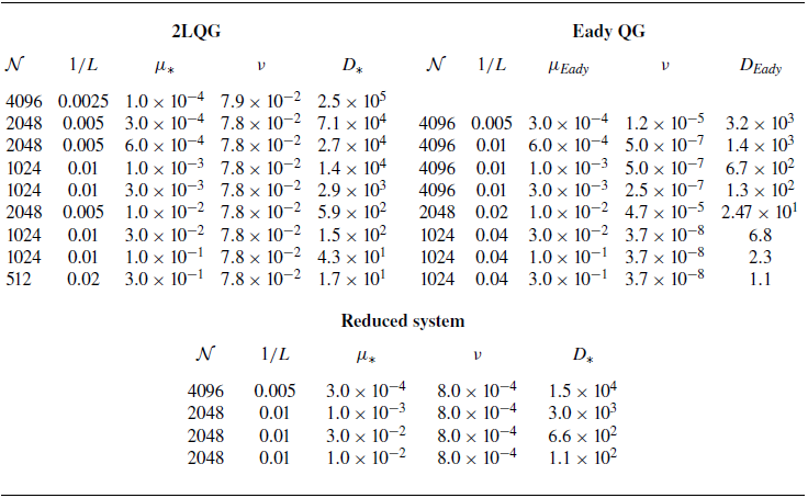
Simulation parameters for the 2LQG model, the QG Eady model and the reduced system, including the resolution
 $\mathcal N$
along each horizontal direction, the inverse dimensionless domain size
 $1/L$
, the dimensionless drag coefficient
 $\mu _{*,{Eady}}$
, the dimensionless hyperviscosity
 $\nu$
, and the measured dimensionless eddy diffusivity
 $D_{*,{Eady}}$
in statistically steady state.

Table 2. Long description
The table compares simulation parameters for the 2LQG model, the QG Eady model, and the reduced system. It includes resolution, inverse dimensionless domain size, dimensionless drag coefficient, dimensionless hyperviscosity, and measured dimensionless eddy diffusivity. The table has three main sections: 2LQG, Eady QG, and Reduced system, each with multiple rows of data. For example, in the 2LQG section, the first row shows N as 4096, 1/L as 0.0025, μ as 1.0 x 10^-4, ν as 7.9 x 10^-2, and D as 2.5 x 10^5. The Eady QG section follows a similar format, and the Reduced system section also lists corresponding parameters.
Acknowledgements
We thank M. Lobo and two anonymous referees for their insightful comments that helped to improve the overall presentation of this work.
Funding
This research is supported by the European Research Council under grant agreement 101124590. This work has benefited from HPC resources from GENCI-IDRIS (Grant 2025-AD012A16265).
Declaration of interests
The authors report no conflict of interest.
Appendix A. Simulation parameters
The parameter values of all simulations are reported in table 2. As described in § 2, the dimensionless domain size is
 $L={\mathcal L}/\lambda$
for the 2LQG model and the reduced model, while it is
 $L={\mathcal L} f/(NH)$
for the Eady model. The spatial resolution along each horizontal direction is denoted by
 $\mathcal N$
. The numerical simulations are performed using a GPU-based pseudo-spectral solver, the details of which can be found in Hadjerci & Gallet (Reference Hadjerci and Gallet2023). The domain size
 $L$
and the dimensionless hyperviscosity
 $\nu$
are adjusted to ensure that the effective diffusivity
 $D_{*,{Eady}}$
is independent of these two parameters. The resolution
 $\mathcal N$
is chosen high enough for the hyperviscous cut-off wavenumber to remain well below the maximum wavenumber
 ${\mathcal N}/3$
, thereby preventing any spurious accumulation at small scale.


 f
 z

 λ

 ℓ∗
 1
 ℓ∗≫1
 ℓ∗∼μ∗−2/3

 Sτ→ψ(k)
 D∗∼μ∗−4/3
 μ∗
 kΩ
 k0.9
 90
 k⩽k0.9

 τ
 τ~=12(p0−p−1)
 Δψ
 U/λ
 b−1−b0
 HSN
 μ∗=3×10⁻⁴
 μEady=6×10⁻⁴
 μEady/3≃3.5×10−4

 D∗/12
 3μ∗
 −4/3

 N
 1/L
 μ∗,Eady
 ν
 D∗,Eady


