2.1. Key parameters

The plume is driven by a buoyancy source at the bottom and grows in a rectangular domain that rotates along the $z\hbox {-}$ axis at rate $\varOmega$ . Since we focus on the fully developed plume that is independent of diffusivity and viscosity, we expect five free parameters determining the plume dynamics, $L,H,r_{ { s}},F_0,f$ . Here, $L$ and $H$ are the width and height of the domain, $r_{ { s}}$ is the radius of the source as the ‘point’ source is actually a finite circular area, $F_0$ (with units m $^{4}$ s $^{-3}$ ) is the buoyancy flux imposed at the source, and $f=2\varOmega$ is the Coriolis parameter.

The dynamics of the rotating point plumes, where the source size $r_{ { s}}$ is small enough to be approximated as a geometric point, is primarily governed by $F_0$ and $f$ . These two physical parameters define a length scale

(2.1) \begin{equation} L_{ \!\textit{ rot}}^p=\left (\frac {F_0}{f^3}\right )^{\frac{1}{4}}, \end{equation}

where the superscript $p$ indicates a point plume. This rotational length scale has been used extensively to describe the characteristic scale of convective plumes in a rotating regime, such as by Speer & Marshall (Reference Speer and Marshall1995), Fernando et al. (Reference Fernando, Chen and Ayotte1998) and Bire et al. (Reference Bire, Mittal, Kang, Ramadhan, Tuckman, German, Thurnherr and Marshall2023).

Naturally, the system can be non-dimensionlised using $L_{ \!\textit{ rot}}^p$ , yielding the dimensionless parameters

(2.2) \begin{equation} \left (\widehat {L},\widehat {H},\widehat {r}_{ { s}}\right )\equiv \left (\frac {L}{L_{ \!\textit{ rot}}^p},\frac {H}{L_{ \!\textit{ rot}}^p},\frac {r_{ { s}}}{L_{ \!\textit{ rot}}^p}\right )\!. \end{equation}

Hereafter, $\widehat { ({\cdot })}$ denotes dimensionless parameters. The point source corresponds to $\widehat {r}_{ { s}}\ll 1$ , so its geometry is negligible. Instead of using $\widehat {L}$ and $\widehat {H}$ , the following two dimensionless numbers are more commonly used and more convenient for analyses:

(2.3) \begin{equation} (\varGamma ,Ro^{*p})\equiv \left (\frac {L}{H},\frac {L_{ \!\textit{ rot}}^p}{H}\right )\!, \end{equation}

where $\varGamma$ is the domain aspect ratio, and $Ro^{*p}$ describes the extent to which rotation dominates the dynamics when the plume reaches the surface at height $H$ (Goodman et al. Reference Goodman, Collins, Marshall and Pierrehumbert2004; Goodman & Lenferink Reference Goodman and Lenferink2012; Bire et al. Reference Bire, Mittal, Kang, Ramadhan, Tuckman, German, Thurnherr and Marshall2023). This $Ro^{*p}$ is often referred to as a natural Rossby number, since the characteristic velocity of rotating plumes is typically scaled by $L_{ \!\textit{ rot}}^pf$ , making $Ro^{*p}$ equivalent to the Rossby number (Jones & Marshall Reference Jones and Marshall1993).

When the source size is non-negligible, i.e. $\widehat {r}_{ { s}}\gtrsim 1$ , the buoyancy flux per unit area should be the key parameter determining plume dynamics. In this circumstance, the rotational length scale can be formulated as

(2.4) \begin{equation} L_{ \!\textit{ rot}}^a=\left (\frac {F_0}{r_{ { s}}^2f^3}\right )^{\frac{1}{2}}\!, \end{equation}

where the superscript $a$ represents per unit area. This $L_{ \!\textit{ rot}}^a$ has been commonly used in studies of convection driven by wide and homogeneous buoyancy sources (e.g. Stone Reference Stone1968; Fernando, Chen & Boyer Reference Fernando, Chen and Boyer1991; Bire et al. Reference Bire, Kang, Ramadhan, Campin and Marshall2022).

In §§ 3 and 4, we focus on the former case, where the buoyancy source can be treated as a geometric point, and the influence of the source radius on the plume dynamics is explored further in § 5.

2.2. Model description and simulation design

We perform high-resolution simulations for rotating hydrothermal plumes using Oceananigans.jl, a GPU-based model that solves non-hydrostatic equations (Ramadhan et al. Reference Ramadhan, Wagner, Hill, Campin, Churavy, Besard, Souza, Edelman, Ferrari and Marshall2020)

(2.5) \begin{align}&\qquad\qquad\quad \boldsymbol{\nabla }\boldsymbol{\cdot }\boldsymbol{u}=0, \end{align}

(2.6) \begin{align} \frac {\partial \boldsymbol{u}}{\partial t}&=-\boldsymbol{u}\boldsymbol{\cdot }\boldsymbol{\nabla }\boldsymbol{u}-f\boldsymbol{k}\times \boldsymbol{u}+b\boldsymbol{k}+\nu {\nabla} ^2\boldsymbol{u}, \end{align}

(2.7) \begin{align} \frac {\partial b}{\partial t}&=-\boldsymbol{u}\boldsymbol{\cdot }\boldsymbol{\nabla }b+\kappa {\nabla} ^2b, \end{align}

where $\boldsymbol{u}=(u,v,w)$ is the three-component velocity, $\boldsymbol{k}$ is the unit vector along the $z$ -axis, $b$ is the buoyancy, and $\nu$ and $\kappa$ are viscosity and diffusivity, respectively.

Rather than adopting an explicit subgrid-scale turbulence closure as in conventional large eddy simulations (LES), we utilise the high-order weighted, essentially non-oscillatory (WENO; Shu Reference Shu2009) advection scheme to stabilise the solution, which is implemented in Oceananigans.jl. This scheme acts as an implicit, adaptive hyper-viscosity mechanism that provides dissipation based on the local smoothness of the solution, which is usually categorised as an implicit LES framework (Grinstein, Margolin & Rider Reference Grinstein, Margolin and Rider2007; Karaca, Lardjane & Fedioun Reference Karaca, Lardjane and Fedioun2012; Pressel et al. Reference Pressel, Mishra, Schneider, Kaul and Tan2017). By relying on the WENO scheme, this model avoids the need to tune uncertain free parameters, and retains effective resolution of turbulence even at lower grid resolutions (Silvestri et al. Reference Silvestri, Wagner, Campin, Constantinou, Hill, Souza and Ferrari2024).

Our domain spans from $-L/2$ to $L/2$ in both the $x$ - and $y$ -directions with doubly periodic boundary conditions. This set-up is intended to represent a scenario in which a cluster of hydrothermal vents is evenly distributed over an extended surface area. Caution needs to be taken if the application’s configuration is different. In the vertical direction ( $z$ -direction), our domain covers $z=0$ to $z=H$ . The rotation rate is set to $\varOmega$ along the $z$ -axis. The initial velocity and buoyancy are both set to zero. At the top, we adopt a stress-free condition for velocity and a no-flux condition for buoyancy, i.e.

(2.8) \begin{equation} w=0,\quad \frac {\partial ^2w}{\partial z^2}=0,\quad \frac {\partial b}{\partial z}=0\qquad \mathrm{at}\ z=H. \end{equation}

This corresponds to a scenario where the rate of heat exchange with the top surface is much slower compared to the motion and evolution of the plume (Goodman & Lenferink Reference Goodman and Lenferink2012). At the bottom, we still adopt a stress-free condition for velocity, but prescribe a steady, axis-symmetric, Gaussian-like buoyancy flux $F$ :

(2.9) \begin{equation} w=0,\quad \frac {\partial ^2w}{\partial z^2}=0,\quad F(x,y)=F_A\exp \left (-\frac {x^2+y^2}{r_{ { s}}^2}\right )\qquad \mathrm{at}\ z=0, \end{equation}

where $F_A$ (with units m $^2$ s $^{-3}$ ) is the maximum buoyancy flux per unit area. The total buoyancy flux is thus given by

(2.10) \begin{equation} F_0=\iint F(x,y)\,\mathrm{d}x\mathrm{d}y=\unicode{x03C0} r_{ { s}}^2F_A. \end{equation}

In this rotating-plume system, two types of instabilities play a role in the plume development. The first is the Kelvin–Helmholtz instability (KHI), which occurs during the initial stage, and triggers the transition from a laminar state to a turbulent state (Kitamura & Sumita Reference Kitamura and Sumita2011; Ward Reference Ward2022). The second instability is baroclinic instability (BCI), which occurs after the plume fully develops (Fernando et al. Reference Fernando, Chen and Ayotte1998; Goodman et al. Reference Goodman, Collins, Marshall and Pierrehumbert2004), and drives lateral mixing between the plume and the ambient fluid. Capturing both instabilities is challenging as BCI occurs at much larger length scales than KHI. To proceed, we set a non-uniform mesh that is refined near the source and gradually coarsens in the upper domain. The dimensionless horizontal and vertical grid sizes, $\widehat {\varDelta }_h$ and $\widehat {\varDelta }_z$ , are given by

(2.11) \begin{equation} \widehat {\varDelta }_h\equiv \frac {\varDelta _h}{L_{ \!\textit{ rot}}^p}=0.04,\quad\widehat {\varDelta }_z\equiv \frac {\varDelta _z}{L_{ \!\textit{ rot}}^p}=\left \{\!\! \begin{array}{ll} 0.02 & 1\leqslant N_z\leqslant 300, \\ 0.02\times 1.01^{(N_z-300)} &301\leqslant N_z\leqslant 450, \\ 0.02\times 1.01^{150} & 451\leqslant N_z\leqslant 1050, \end{array} \right . \end{equation}

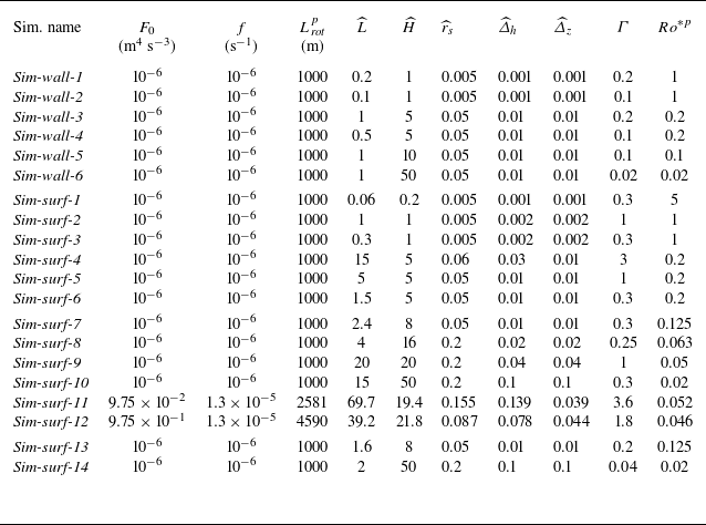
where $N_z$ denotes the vertical grid index, and subscripts $h$ and $z$ refer to horizontal and vertical directions, respectively. The total number of grid cells is 486 in both $x$ - and $y$ -directions, and is 1050 in the vertical, resulting in dimensionless domain size $\widehat {L}=19.44$ and $\widehat {H}=66.34$ . One simulation using this refined mesh is conducted as the reference case, which is referred to as Sim-refine (table 1). The results of this simulation are presented in figure 1. However, due to computational resource limitations, most simulations are performed on a uniform mesh with somewhat lower resolution (tables 1 and 2). The reduced resolution may delay the onset of KHI due to a compromised ability to resolve small-scale turbulence (i.e. the WENO scheme leads to larger numerical diffusivity and viscosity), potentially affecting the subsequent onset of BCI and our main results. To assess the numerical convergence with respect to resolution, a grid sensitivity analysis is presented in § 3.4.

Table 1.

Summary of parameters used in the numerical simulations for free plumes discussed in § 3: names of simulations, buoyancy flux $F_0$ , Coriolis parameter $f$ , rotational length scale $L_{ \!\textit{ rot}}^p$ , dimensionless (hereafter) domain width $\widehat {L}$ and height $\widehat {H}$ , source radius $\widehat {r}_{ { s}}$ , horizontal and vertical grid sizes $\widehat {\varDelta }_h$ and $\widehat {\varDelta }_z$ , domain aspect ratio $\varGamma$ , and natural Rossby number $Ro^{*p}$ . Parameters in Sim-repeat are the same as one simulation in Bire et al. (Reference Bire, Mittal, Kang, Ramadhan, Tuckman, German, Thurnherr and Marshall2023).

2.3. Diagnosis of plume morphology

To diagnose the height and width of the plume, we first compute the buoyancy field averaged along the $y$ -direction, and then diagnose the envelope of the plume $\mathcal{C}$ following

(2.12) \begin{equation} \mathcal{C}(t)\equiv \left \{(x,z)\,\bigg |\,\frac {\overline {b}^y}{\overline {b}^y_s}=0.1\, \%\right \}\!, \end{equation}

where $\overline {({\cdot })}^y$ denotes the average along the $y$ -direction, and the subscript $s$ indicates calculation at the source. This approach, equivalent to a side-view perspective, minimises the need to store large three-dimensional datasets, and ensures that the farthest plume front is captured regardless of its position. In this way, the plume height $h_{ { p}}$ is then diagnosed as the height of the highest point on $\mathcal{C}$ , and the plume width $d_{ { p}}$ is diagnosed as the horizontal distance between the minimum and maximum $x$ -coordinates on $\mathcal{C}$ , i.e.

(2.13) \begin{equation} h_{ { p}}\equiv \max(z(\mathcal{C})),\quad d_{ { p}}\equiv \max(x(\mathcal{C}))-\min(x(\mathcal{C})). \end{equation}

Figure 1.

The three development stages of a free rotating point plume in an unstratified environment. (a) Diagram of three stages during a plume’s growth. (b–g) Instantaneous snapshots of the dimensionless buoyancy in the simulation Sim-refine in table 1: (b–d) side view, (e–g) bird’s-eye view. Superscripts $y$ and $z$ denote averaging along the $y$ - and $z$ -directions, respectively. In each panel, the theoretical predictions of geometry (if they exist) are represented by black dashed curves. (h–j) Vertical profiles of scaled vertical velocity (blue) and buoyancy (green) at the plume centre. Dashed curves represent theoretical predictions ( $W$ and $B$ , if they exist), and solid curves represent simulated results ( $W_{sim}$ and $B_{sim}$ ). In (h), the vertical velocity and buoyancy are scaled by $W(L_{ \!\textit{ rot}}^p)$ and $B(L_{ \!\textit{ rot}}^p)$ calculated from (3.2) and (3.3), respectively. In (i) and ( j), they are scaled by $w_{ { c}}$ and $b_{ { c}}$ from (3.8) and (3.9), respectively.

Table 2.

Same as table 1, but for plumes constrained by boundaries discussed in § 4. Parameters in Sim-surf-11 and Sim-surf-12 are the same as simulations shown in figures 2 and 3 in Goodman & Lenferink (Reference Goodman and Lenferink2012).

The 0.1 % threshold is chosen as it captures the bulk of the convective plume while minimising the influence of diffusion at the edges. Our results in this study are insensitive to the choice of the threshold, as the transition from a finite $b$ to zero occurs in a very narrow spatial region (see supplementary figures S1 and S2).

3.1. Stage-1: free-turbulent plume

In the first stage, the buoyant fluid emanating from the source is not yet influenced by rotation, so the plume is filled by three-dimensional turbulence. These turbulent motions entrain dense ambient fluid into the plume, reducing its buoyancy and vertical velocity while expanding laterally to form a cone shape (stage-1 in figure 1 a).

During this stage, $F_0$ is the only external dimension parameter that determines the plume. As shown in MTT, the radius of the plume $R$ , the upwelling velocity $W$ , and buoyancy anomaly $B$ at the plume centre follow

(3.1) \begin{align} R(z)&=\frac {6}{5}\alpha z\approx 0.11z, \end{align}

(3.2) \begin{align} W(z)&=\frac {5}{6\alpha }\left [\frac {9\alpha }{5}\left (\frac {2F_0}{\unicode{x03C0} }\right )\right ]^{\frac{1}{3}}z^{- \frac{1}{3}}\approx 4.25 (F_0z^{-1})^{\frac{1}{3}}\!, \end{align}

(3.3) \begin{align} B(z)&=\frac {5}{6\alpha }\left [\frac {9\alpha }{5}\left (\frac {2F_0}{\unicode{x03C0} }\right )\right ]^{- \frac{1}{3}}\left (\frac {2F_0}{\unicode{x03C0} }\right )z^{-\frac {5}{3}}\approx 12 (F_0^2z^{-5})^{\frac{1}{3}} \!, \end{align}

where $\alpha$ is the entrainment coefficient ( $=0.093$ for buoyant plume; Morton et al. Reference Morton, Taylor and Turner1956). Also, we can obtain a volume flux $\mu$ and a momentum flux $m$ from MTT:

(3.4) \begin{align} \mu (z)&=\frac {6\alpha \unicode{x03C0} }{5}\left [\frac {9\alpha }{5}\left (\frac {2F_0}{\unicode{x03C0} }\right )\right ]^{\frac{1}{3}}z^{\frac{5}{3}}\approx 0.17 (F_0z^5)^{\frac{1}{3}}, \end{align}

(3.5) \begin{align} m(z)&=\frac {\unicode{x03C0} }{2}\left [\frac {9\alpha }{5}\left (\frac {2F_0}{\unicode{x03C0} }\right )\right ]^{ \frac {2}{3}}z^{\frac{4}{3}}\approx 0.35(F_0z^2)^{\frac{2}{3}}, \end{align}

which align with the measurements from laboratory experiments (Rouse et al. Reference Rouse, Shun Yih and Humphreys1952; List & Imberger Reference List and Imberger1973; List Reference List1982).

The evolution of the plume in the reference case Sim-refine is shown in figure 1. In the early stage after model initialisation, a free-turbulent plume is observed (figure 1 b). This plume occupies a clearly defined cone shape, which aligns with that predicted by (3.1). Figure 1(h) shows the vertical profiles of vertical velocity and buoyancy measured along the centre of the plume, $W(z)$ and $B(z)$ , both of which decrease as the plume rises and align with (3.2) and (3.3).

Note that $W(z)$ and $B(z)$ become singular at $z=0$ , indicating that the MTT model is invalid near the source, as the source cannot be treated as a point there. For a circular source with finite area, the point plume assumption and the MTT model have been shown to be valid only when $z\gt 24r_{ { s}}$ (Fernando et al. Reference Fernando, Chen and Ayotte1998). In our results, the invalid region is highlighted in grey in figure 1(h). Within this region, our simulation results indeed depart notably from the MTT prediction. Specifically, $W(z)$ is observed to be zero near the bottom due to boundary effects, whereas the theoretical prediction is infinite.

3.2. Stage-2: rotation-dominated cylindrical plume

As the plume evolves, rotational effects become significant, deflecting the originally radial inflow to generate a rim current around the plume. This process limits the volume of fluid that can be entrained, as fluid farther away is blocked from entering the plume, which effectively inhibits lateral material/buoyancy exchange between the plume and the ambient fluid. Therefore, the radius of the plume remains almost constant, as can be seen in stage-2 in figure 1(a). The rim current speed is such that it is in thermal wind balance with the buoyancy contrast inside and outside the plume (Legg, Jones & Visbeck Reference Legg, Jones and Visbeck1996; Fernando et al. Reference Fernando, Chen and Ayotte1998; Goodman et al. Reference Goodman, Collins, Marshall and Pierrehumbert2004).

In this stage, the external parameters that determine the plume are $F_0$ and $f$ , which can be combined into $L_{ \!\textit{ rot}}^p$ (see (2.1)). When the plume is $O(L_{ \!\textit{ rot}}^p)$ away from the source, the Rossby number $Ro\equiv {W}/{fR}$ drops below unity, demarcating the transition from the non-rotating to the rotating regime (Ma et al. Reference Ma, Flynn and Sutherland2020). Following Fernando et al. (Reference Fernando, Chen and Ayotte1998) and Goodman et al. (Reference Goodman, Collins, Marshall and Pierrehumbert2004), the transitional height $h_{ { c}}$ and the radius of the cylinder $r_{ { c}}$ follow

(3.6) \begin{align} h_{ { c}}&\approx 6.0L_{ \!\textit{ rot}}^p, \end{align}

(3.7) \begin{align} r_{ { c}}&\approx 0.7L_{ \!\textit{ rot}}^p. \end{align}

Within the plume, the vertical velocity and buoyancy are nearly homogeneous and remain constant as the plume rises. They can be estimated from the MTT solution at $z=h_{ { c}}$ :

(3.8) \begin{align} w_{ { c}}&\approx \frac {\mu (h_{ { c}})}{\unicode{x03C0} r_{ { c}}^2}\approx 2.2L_{ \!\textit{ rot}}^pf, \end{align}

(3.9) \begin{align} b_{ { c}}&\approx \frac {F_0}{\mu (h_{ { c}})}\approx 0.3L_{ \!\textit{ rot}}^pf^2. \end{align}

These scaling laws are found to align with previous lab experiments (Fernando et al. Reference Fernando, Chen and Ayotte1998; Goodman et al. Reference Goodman, Collins, Marshall and Pierrehumbert2004) and numerical simulations (Goodman & Lenferink Reference Goodman and Lenferink2012).

Figure 1(c) shows a snapshot at $t=9f^{-1}$ (where $t=4\unicode{x03C0} f^{-1}$ corresponds to one rotation period) in the reference simulation. Below the level of $z=6L_{ \!\textit{ rot}}^p$ , the plume retains a conical shape. However, above this level, the plume is strongly influenced by rotation, taking on a cylindrical shape with radius approximately $1.2L_{ \!\textit{ rot}}^p$ . This shape aligns with the predictions of (3.6) and (3.7), as indicated by the black dashed lines. The slight discrepancy in plume radius may result from the modification of the entrainment coefficient by rotation. In the cylindrical region, vertical velocity and buoyancy become well mixed both horizontally and vertically, broadly matching the theoretical values given by (3.8) and (3.9), as shown in figure 1(i).

However, this stage is short-lived for two reasons. First, the plume near the source exhibits more complex dynamics. It may re-enter a laminar state due to the suppression of turbulence by rotation (Sutherland et al. Reference Sutherland2021), or it may be quickly deflected from the vertical, beginning to precess and oscillate due to the adverse pressure gradient encountered in the rotating environment (Frank et al. Reference Frank, Landel, Dalziel and Linden2017; Ma et al. Reference Ma, Flynn and Sutherland2020; Sutherland et al. Reference Sutherland2021; see also supplementary figure S3). This leads to meandering and expansion of the cylindrical plume above. Second, BCI develops, with baroclinic eddies mixing the plume with the surrounding fluid, further driving lateral expansion, as discussed in the next subsection.

3.3. Stage-3: destabilised plume

The rotation-governed cylindrical plume becomes unstable due to barotropic or baroclinic instabilities (of the rim current), in line with Kang et al. (Reference Kang, Marshall, Mittal and Bire2022a ) and Bire et al. (Reference Bire, Mittal, Kang, Ramadhan, Tuckman, German, Thurnherr and Marshall2023). After that, the plume will expand horizontally, as eddies scatter the plume fluid into the surrounding environment (stage-3 in figure 1 a). In our simulations, the destabilisation of the cylindrical plume is observed, as the plume spreads horizontally throughout the domain, with its horizontal extent far exceeding $r_{ { c}}$ (figure 1 d,g), and its vertical velocity and buoyancy substantially decreasing (figure 1 j).

Figure 2.

Evolution of (a) the plume height $h_{ { p}}$ and (b) the width $d_{ { p}}$ in the series of simulations labelled Sim-free in table 1. The time $t$ is scaled by $f^{-1}$ , and $h_{ { p}}$ and $d_{ { p}}$ are scaled by $L_{ \!\textit{ rot}}^p$ . In (a), the black dashed line and the grey region represent (3.10). In (b), the black dashed line represents the scaling $(\kern1.5pt \textit{ft})^{1/2}$ .

In the simulations listed in table 1, the destabilised plumes eventually stop growing in height, despite the absence of stratification. Figure 2(a) shows the evolution of plume height for cases in Sim-free, and it is clear that all plumes plateau at a final height $h_{ \!{ f}}$ :

(3.10) \begin{equation} h_{ \!{ f}}\approx (55\pm 5)L_{ \!\textit{ rot}}^p, \end{equation}

which scales with $L_{ \!\textit{ rot}}^p$ . This plateau occurs around $t=100f^{-1}$ , and from then on, the plumes only expand laterally, following $d_{ { p}}\sim L_{ \!\textit{ rot}}^p(\kern1.5pt \textit{ft})^{1/2}$ as shown in figure 2(b). This phenomenon has also been observed in a fast-rotating ( $Ro^{*p}=1/59$ ) tank experiment conducted by Goodman et al. (Reference Goodman, Collins, Marshall and Pierrehumbert2004), and in numerical simulations for very deep subsurface oceans in icy worlds performed by Kang et al. (Reference Kang, Marshall, Mittal and Bire2022a ) and Bire et al. (Reference Bire, Mittal, Kang, Ramadhan, Tuckman, German, Thurnherr and Marshall2023). The breakdown of concentrated plumes is particularly important for icy worlds, as it dictates whether heat and materials from the vent can be transported to the ice shell without significant dilution.

Here, we propose a physical explanation for the destabilisation. Inspired by Brickman (Reference Brickman1995), Legg et al. (Reference Legg, Jones and Visbeck1996) and Visbeck, Marshall & Jones (Reference Visbeck, Marshall and Jones1996), we hypothesise that the plume will stop growing when the lateral buoyancy scattering by eddies balances out the buoyancy injection from the source:

(3.11) \begin{equation} \int _0^{h_{ \!{ f}}}\overline {u'b'}\times2\unicode{x03C0} r\mathrm{d}z=F_0. \end{equation}

Here, $r$ is the radius of the expanded plume, $u'$ is the radial eddy velocity, $b'$ is the buoyancy perturbation, and $\overline {({\cdot })}$ denotes azimuthal averaging. By definition, $\overline {u'}=0$ and $\overline {b'}=0$ , but $\overline {u'b'}$ is non-zero because $u'$ and $b'$ are correlated. Following Legg et al. (Reference Legg, Jones and Visbeck1996), we estimate this lateral eddy buoyancy flux as $u^* \Delta b$ , where $u^*$ is the root mean square of $u'$ , and $\varDelta b$ is the buoyancy contrast between the plume and environment (equal to the buoyancy within the plume $b_{ { p}}$ ). Therefore, to estimate this eddy flux, we need scales for $u^*$ and $b_{ { p}}$ . According to the linear instability approach pioneered by Eady (Reference Eady1949) and Stone (Reference Stone1972), and later applied by Legg et al. (Reference Legg, Jones and Visbeck1996) to plumes, we estimate that $u^*$ scales with the rim current speed $U_{ \textit{rim}}$ as

(3.12) \begin{equation} u^*=\gamma U_{ \textit{rim}}, \end{equation}

where $\gamma$ is a constant coefficient. The rim current speed $U_{ \textit{rim}}$ can be related to $b_{ { p}}$ through the thermal wind balance (see supplementary figure S4):

(3.13) \begin{equation} \frac {\partial U_{ \textit{rim}}}{\partial z}=-\frac {1}{f}\frac {\partial b}{\partial r}\ \Rightarrow \ U_{ \textit{rim}}=\frac {zb_{ { p}}}{\textit{fr}}. \end{equation}

For $b_{ { p}}$ , we assume that it is well mixed within the plume, and is diluted from $b_{ { c}}$ due to the plume expansion (e.g. figure 1 d,g,j). Thus it can be scaled as

(3.14) \begin{equation} b_{ { p}}=CL_{ \!\textit{ rot}}^pf^2, \end{equation}

where $C=0.3r_{ { c}}^2/r^2$ . Here, we have used (3.9). Substituting all equations into the buoyancy budget (3.11), we obtain

(3.15) \begin{equation} h_{ \!{ f}}=\frac {1}{\sqrt {\unicode{x03C0} \gamma }\,C}L_{ \!\textit{ rot}}^p. \end{equation}

From numerical simulations, Legg et al. (Reference Legg, Jones and Visbeck1996) estimated $\gamma \approx 0.25$ for plumes in an unstratified environment. Also, in our simulations, the plume radius is approximately $1.2L_{ \!\textit{ rot}}^p$ during the early cylindrical stage, and expands to approximately $5L_{ \!\textit{ rot}}^p$ when it begins to stop ascending (figure 2 b), giving $C\approx 0.02$ . Substituting these values into (3.15) yields

(3.16) \begin{equation} h_{ \!{ f}}\approx 60L_{ \!\textit{ rot}}^p, \end{equation}

which quantitatively agrees with the measurements in our simulations.

In addition, since $\overline {u'}=0$ , there is no net lateral eddy volume flux, so the volume of the plume $V_{ { p}}$ can be estimated as

(3.17) \begin{equation} V_{ { p}}=\mu (\kern1.5pt \textit{ft})t=\widehat {\mu }(\kern1.5pt \textit{ft}) \big(L_{ \!\textit{ rot}}^p \big)^3ft, \end{equation}

where $\mu (\kern1.5pt \textit{ft})$ (with dimensionless form $\widehat {\mu }$ ) represents the volume flux entrained during the MTT stage (stage-1), which remains a constant after the plume enters stage-2. This rate scales with $(L_{ \!\textit{ rot}}^p)^3 f$ as this is the only way to construct a physical variable with unit m $^3$ s $^{-1}$ . Noticing that after plume height plateaus, the plume volume can be expressed as $d_{ { p}}^2h_{ \!{ f}}$ , a scaling for $d_p$ can be obtained:

(3.18) \begin{equation} d_{ { p}}^2L_{ \!\textit{ rot}}^p\sim (L_{ \!\textit{ rot}}^p)^3 \textit{ft}\quad \Rightarrow \quad\frac {d_{ { p}}}{L_{ \!\textit{ rot}}^p}\sim (\kern1.5pt \textit{ft})^{\frac{1}{2}}, \end{equation}

which is consistent with the evolution of $d_{ { p}}$ shown in figure 2(b).

3.4. Sensitivity test

In our simulations, due to computational limitations, turbulent energy dissipates at the grid scale, which is significantly larger than the Kolmogorov scale. This may influence the growth of turbulent plumes. To assess whether and to what extent the model resolution affects our conclusions, we perform a mesh sensitivity study in this subsection. We vary $\widehat {\varDelta }_h$ and $\widehat {\varDelta }_z$ in a series of simulations labelled Sim-res in table 1. This variation effectively modifies the diffusivity and viscosity while maintaining a fixed resolution.

Figure 3.

Middle row: final penetration height $h_{ \!{ f}}$ on meshes with different dimensionless (vertical) resolutions in simulations labelled Sim-refine and Sim-res in table 1. As a comparison, the resolution ranges in Sim-free (blue), Sim-wall (green) and Sim-surf (red) are marked on the $x$ -axis. Data points represent the average over the time interval from $ft=100$ to $ft=200$ , with error bars indicating the maximum and minimum values within this interval. The black dashed line and grey shading represent $(55\pm 5)L_{ \!\textit{ rot}}^p$ . Upper and lower rows: side views of the plume shape during its evolution in simulations Sim-res-4 and Sim-refine, respectively. In the lower row, grey shading covers the region out of the domain. Several insets are included. Theoretical geometry predictions (if they exist) are represented by dashed curves.

Lower resolution delays the onset of KHI and overestimates the height at which the plume transitions to a turbulent state, as illustrated in figure 3. Initially, the plume remains laminar due to the low Reynolds number $\textit{Re}$ , then it transits to the turbulent state as $\textit{Re}$ increases. This transition, induced by KHI, has been observed in previous laboratory experiments (e.g. Kitamura & Sumita Reference Kitamura and Sumita2011), simulations by general circulation models (e.g. Goodman & Lenferink Reference Goodman and Lenferink2012), and direct numerical simulations (e.g. Ward Reference Ward2022). The critical height and time for this transition are found to scale with

(3.19) \begin{equation} L_{\kappa }\equiv \left (\frac {\kappa ^3}{F_0}\right )^{\frac{1}{2}}\!,\quad t_{\kappa }\equiv \frac {\kappa ^2}{F_0}, \end{equation}

where $\kappa$ is the diffusivity (Ward Reference Ward2022). In low-resolution simulations, turbulent energy dissipates at larger scales, leading to larger effective $\kappa$ . This delays the onset of KHI and allows the laminar plume to penetrate to higher heights, potentially exceeding $h_{ { c}}$ (top left panel in figure 3). Consequently, the MTT stage does not emerge, and the plume transits directly into a rotationally dominant cylinder (top right panel in figure 3). As resolution increases, smaller-scale turbulence is better resolved, leading to an earlier onset of KHI and the transition to the turbulent plume. This allows the MTT stage to develop and be captured accurately (lower row in figure 3).

Furthermore, lower resolution overestimates the final penetration height $h_{ \!{ f}}$ , as shown in the middle row of figure 3. This is because the laminar plume in the earlier stage penetrates too high (top left panel in figure 3). Additionally, a lower-resolution mesh has a reduced ability to resolve small-scale baroclinic eddies, leading to an underestimate of lateral eddy buoyancy flux, which also contributes to a higher penetration height. As the resolution increases, $h_{ \!{ f}}$ converges to approximately $55L_{ \!\textit{ rot}}^p$ , demonstrating that the mesh adopted before with $\widehat {\varDelta }_h=\widehat {\varDelta }_z=0.1$ is sufficient to capture the destabilised plume induced by BCI, while minimising the influence of variations in the onset time of KHI. Consequently, the measured $h_{ \!{ f}}$ in (3.10) is robust.

We also adopt different domain extents $\widehat {L}$ and $\widehat {H}$ in Sim-refine, Sim-free-8, Sim-free-9 and Sim-res-1. The similar plume evolution and $h_{ \!{ f}}$ shown in figure 2 demonstrate that these domain sizes are sufficient to ensure that the plume is not influenced by boundaries.

4.1. Lateral-constrained regime

To investigate the plume pattern that will first encounter lateral boundaries (equivalent to interactions with other plumes), we carried out six simulations that satisfy the criterion for the lateral-constrained regime, labelled Sim-wall in table 2. The plumes in these simulations exhibit similar behaviour (bottom right panels in figure 4).

Snapshots of $b/b_{s}$ at different time steps in Sim-wall-5 are illustrated in figure 5. The plume is found to encounter the lateral boundaries at $z\approx 4L_{ \!\textit{ rot}}^p$ , consistent with the prediction of MTT. Thereafter, the plume merges with adjacent plumes and becomes horizontally well mixed. This indicates that fluid above this level only ‘sees’ a uniformly distributed buoyancy flux, regardless of the buoyancy flux pattern at the bottom. Over time, these plumes first fill the lower part of the domain with high-buoyancy fluid. This occurs because the plume’s upwelling must be balanced by surrounding downwelling. After plumes fill the horizontal extent of the domain, the compensating downward motions occur near the domain side walls, pushing high-buoyancy fluid. This behaviour resembles the ‘filling-box’ effect described by Baines & Turner (Reference Baines and Turner1969) and Turner (Reference Turner1969). Only after the lower domain becomes well mixed does the high-buoyancy fluid begin to fill the upper domain.

4.2. Top-constrained regimes

To investigate the plume pattern that will first encounter the top boundary, we conduct a series of simulations labelled Sim-surf in table 2, which include both weakly rotating cases (Sim-surf-1 to Sim-surf-6) and strongly rotating cases (Sim-surf-7 to Sim-surf-12).

Figure 5.

Instantaneous $x{-}z$ cross-sections of dimensionless buoyancy $b/b_{s}$ along $y=0$ in the simulation Sim-wall-5 in table 2. Dashed lines represent the plume geometry predicted by MTT model (3.1). To better illustrate the plume structure, the threshold is adjusted to $10^{-4}$ .

If $Ro^{*p}\gt 1/6$ , then rotation has no effect on the rising plume, so the plume maintains the cone shape predicted by the MTT model (3.1) until it meets the upper boundary, as shown in figures 6(a) and 6(d). After that, the buoyant fluid spreads horizontally in appearance of radial gravity currents along the top boundary, forming an anvil layer (figure 6 b,e). This behaviour is similarly reported in tank experiments by Fernando et al. (Reference Fernando, Chen and Ayotte1998). Eventually, if the domain is relatively narrow, the plume will fill the plane and be pushed downwards under the influence of the ‘filling-box’ effect discussed in § 4.1 (figure 6 c,f). In contrast, when sufficient horizontal space is available, the radial gravity currents will eventually be influenced by rotation, deflecting and forming anticyclonic flows around a confined plume, consistent with the phenomena reported by Ma et al. (Reference Ma, Flynn and Sutherland2020) and Bire et al. (Reference Bire, Mittal, Kang, Ramadhan, Tuckman, German, Thurnherr and Marshall2023).

Figure 6.

Instantaneous views of dimensionless buoyancy $b/b_{s}$ (colour shading) and horizontal flows (vectors) in the simulation Sim-surf-2 in table 2: (a–c) $x{-}z$ cross-sections along blue dash-dotted lines in (d–f); (d–f) $x{-}y$ cross-sections at the top. Theoretical geometry predictions (if they exist) are represented by black dashed lines. To better illustrate the plume structure, the threshold is adjusted to $10^{-4}$ .

If $Ro^{*p}\lt 1/6$ , then rotation would have already started to modulate the plume before encountering the top boundary. As demonstrated in Goodman et al. (Reference Goodman, Collins, Marshall and Pierrehumbert2004), in this case, the plume undergoes the first two stages sketched in figure 1(a), and impacts the upper boundary as a cylindrical plume, generating anticyclonic flows (figure 7 a,b,e). Then the cylindrical plume expands outwards by virtue of mass conservation. However, in a rotational system, the range that the outward flow can reach is limited through the onset of a rim current. As a result, plume fluid accumulates near the top boundary, causing the cylindrical plume to evolve into a baroclinic cone (figure 7 a,c,f). The diameter of the cone scales with $L_{ { cone}}=\sqrt {b'H}/f\sim L_{ \!\textit{ rot}}^p/\sqrt {Ro^{*p}}$ (Fernando et al. Reference Fernando, Chen and Ayotte1998; Goodman et al. Reference Goodman, Collins, Marshall and Pierrehumbert2004; Goodman & Lenferink Reference Goodman and Lenferink2012), which is the Rossby deformation radius for a two-layer fluid (Pedlosky Reference Pedlosky1987). We validated this cone scaling (see supplementary figure S5). Finally, due to BCI, the primary cone breaks down into multiple secondary conical vortices (two vortices in figure 7 d,g). The numbers of these vortices can be estimated using a ‘heton’ model, as shown by Legg & Marshall (Reference Legg and Marshall1993) and Legg et al. (Reference Legg, Jones and Visbeck1996).

Figure 7.

Development of a rotating plume after encountering the top boundary. (a) Diagram of three stages during a plume’s growth. (b–g) Same as figure 6 but for the simulation Sim-surf-9 in table 2. In (a), $l$ is the diameter of the conical plume in stage-2. To better illustrate the plume structure, the threshold is adjusted to $10^{-4}$ .