Frequency-tuned surfaces for passive control of wall-bounded turbulent flow – a resolvent analysis study

Azadeh Jafari; Beverley J. McKeon; Maziar Arjomandi

doi:10.1017/jfm.2023.149

Frequency-tuned surfaces for passive control of wall-bounded turbulent flow – a resolvent analysis study

Published online by Cambridge University Press: 22 March 2023

and

Azadeh Jafari*: Affiliation:
School of Mechanical Engineering, University of Adelaide, Adelaide, SA 5005, Australia
Beverley J. McKeon: Affiliation:
Graduate Aerospace Laboratories, California Institute of Technology, 1200 East California Boulevard, Pasadena, CA 91125, USA
Maziar Arjomandi: Affiliation:
School of Mechanical Engineering, University of Adelaide, Adelaide, SA 5005, Australia
*: †Email address for correspondence: azadeh.jafari@adelaide.edu.au

Article contents

Abstract
Introduction
Methodology
Results
Shear-driven vs pressure-driven impedance
Effect of Reynolds number on control performance
Implications for design of frequency-tuned walls
Conclusions
Funding
Declaration of interests
References

Rights & Permissions

Abstract

The potential of frequency-tuned surfaces as a passive control strategy for reducing drag in wall-bounded turbulent flows is investigated using resolvent analysis. These surfaces are considered to have geometries with impedances that permit transpiration and/or slip at the wall in response to wall pressure and/or shear and are tuned to target the dynamically important structures of wall turbulence. It is shown that wall impedance can suppress the modes resembling the near-wall cycle and the very-large-scale motions and the Reynolds stress contribution of these modes. Suppression of the near-wall cycle requires a more reactive impedance. In addition to these dynamically important modes, the effect of wall impedance across the spectral space is analysed by considering varying mode speeds and wavelengths. It is shown that the materials designed for suppression of the near-wall modes lead to gain reduction over a wide range across the spectral space. Furthermore, a wall with only shear-driven impedance is found to suppress turbulent structures over a wider range in spectral space, leading to an overall turbulent drag reduction. Most importantly, the present analysis shows that the drag-reducing impedance is non-unique and the control performance is not sensitive to variations of the surface impedance within a favourable range. This implies that specific frequency bandwidths can be targeted with periodic material design.

JFM classification

Flow Control: Drag reduction

Information

Type: JFM Papers
Information: Journal of Fluid Mechanics , Volume 959 , 25 March 2023, A26
DOI: https://doi.org/10.1017/jfm.2023.149 [Opens in a new window]
Creative Commons: This is an Open Access article, distributed under the terms of the Creative Commons Attribution licence (http://creativecommons.org/licenses/by/4.0/), which permits unrestricted re-use, distribution and reproduction, provided the original article is properly cited.
Copyright: © The Author(s), 2023. Published by Cambridge University Press

1. Introduction

Turbulent skin-friction drag is a major constituent of the total drag in many engineering applications including air, sea, ground and fluid transportation. As an example, approximately half of the total drag on an aircraft is due to skin-friction drag (Gad-el-Hak Reference Gad-el-Hak1994). Hence, due to the significant economic and environmental benefits, reducing skin friction has motivated considerable effort for the control of wall-bounded turbulence, including active and passive control techniques. A particularly attractive passive control concept, requiring no energy input and no complex control algorithms, is taking benefit of the wall material properties through the interaction between the wall and the turbulent flow, examples of which include perforated (Silvestri et al. Reference Silvestri, Ghanadi, Arjomandi, Cazzolato and Zander2017; Bhat et al. Reference Bhat, Silvestri, Cazzolato and Arjomandi2021; Jafari, Cazzolato & Arjomandi Reference Jafari, Cazzolato and Arjomandi2022), permeable (Breugem, Boersma & Uittenbogaard Reference Breugem, Boersma and Uittenbogaard2006; Kuwata & Suga Reference Kuwata and Suga2017; Suga et al. Reference Suga, Okazaki, Ho and Kuwata2018; Chavarin et al. Reference Chavarin, Efstathiou, Vijay and Luhar2020, Reference Chavarin, de Segura, García-Mayoral and Luhar2021) and compliant walls (Lee, Fisher & Schwarz Reference Lee, Fisher and Schwarz1993; Xu, Rempfer & Lumley Reference Xu, Rempfer and Lumley2003; Kim & Choi Reference Kim and Choi2014; Xia, Huang & Xu Reference Xia, Huang and Xu2017). Based on the surface properties, these walls may suppress and/or energise specific frequency bandwidths within the turbulent flow. While some of the previous studies on permeable and compliant walls showed promising results, drag increasing cases, arising from energised large-scale spanwise structures (Jiménez et al. Reference Jiménez, Uhlmann, Pinelli and Kawahara2001; Breugem et al. Reference Breugem, Boersma and Uittenbogaard2006; Kim & Choi Reference Kim and Choi2014; Luhar, Sharma & McKeon Reference Luhar, Sharma and McKeon2015; Kuwata & Suga Reference Kuwata and Suga2017), were also found. The motivation of this study is to explore walls that could be tuned to passively suppress the dynamically important energetic structures of wall turbulence without significantly amplifying other scales, such that these frequency-tuned walls could create an overall reduction in drag.

We consider a general framework in which walls are designed with geometries that permit transpiration and/or slip in response to wall pressure and/or shear, and thus passively interact with the turbulent flow. We seek to determine the potential of such passive walls for reducing turbulent drag, thus shedding light on future surface designs. In the present study, surface impedance is employed to describe the interaction of the frequency-tuned walls with the turbulent flow in terms of a modified wall-boundary condition, i.e. an impedance wall formulation. The surface impedance is commonly used as an effective boundary condition for acoustic analysis of the interactions of a surface with an acoustic field. In classical definitions, surface impedance defines a linear relationship between pressure and the flow velocity normal to the surface, i.e. a pressure-driven impedance. The classical pressure-driven impedance has been used in the literature, in the form of coupled wall-normal and pressure boundary conditions, for modelling of the boundary layer stability and transition over perforated surfaces (Burden Reference Burden1969; Porter Reference Porter1998; Luhar et al. Reference Luhar, Sharma and McKeon2015). While the classical impedance formulation in previous studies correlates the wall-normal velocity and pressure at the wall, it does not account for the presence of viscous flow over the surface. It has been shown in the impedance eduction measurements in the presence of grazing flow (Renou & Aurégan Reference Renou and Aurégan2011; Dai & Auregan Reference Dai and Auregan2016; Boden et al. Reference Boden, Cordioli, Spillere and Serrano2017) that surface impedance is also correlated with the wall shear. Hence, the effect of surface impedance on the turbulent flow can only be fully described if its correlation with wall shear, i.e. wall-shear-driven impedance, is also considered. This is also of significance for design of control strategies as the studies in the literature suggest a potential for passive control driven by wall shear. For example, Fukagata et al. (Reference Fukagata, Kern, Chatelain, Koumoutsakos and Kasagi2008) showed that a compliant wall which could be deformed by both streamwise wall shear stress and pressure could create up to 8 % drag reduction in a turbulent channel flow. Investigating the application of a wall-shear-driven compliant surface with in-plane wall deformations, Józsa et al. (Reference Józsa, Balaras, Kashtalyan, Borthwick and Viola2019) also found that passive streamwise in-plane motions of the wall could create up to 3.8 % drag reduction ($\textit {Re}_{\tau }=180$), while passive spanwise wall fluctuations increased skin friction by more than 50 %. To our knowledge, despite previous studies on pressure-driven passive control, specifically passive walls such as permeable and compliant walls, a generalised theoretical model for pressure/shear-driven impedance walls is lacking.

This study develops a theoretical framework to investigate the interaction between the frequency-tuned walls and turbulent flows incorporating both pressure- and wall-shear-driven impedance. This framework is particularly beneficial for design of passive frequency-tuned walls and provides an understanding of the combined effects of passive pressure-driven and wall-shear-driven control approaches. Furthermore, this bulk approach based on surface impedance permits modelling of a surface with a general geometry without the need to resolve geometric details. The latter not only requires large and strenuous computations, but is also limited to the specific geometries considered. Therefore, using the surface impedance formulation is advantageous for conducting a generalised and thorough analysis of the application of the described walls as a passive control strategy. As the classical impedance formulation only considers pressure-driven control, an improved generalised impedance formulation developed by Gabard (Reference Gabard2020) is adopted in the present study. The generalised impedance defines a linear correlation between surface traction and flow velocity including the effects of mean shear at the surface (Gabard Reference Gabard2020), therefore incorporating both pressure- and wall-shear-driven control schemes into the impedance tensor and considering a surface that allows either or both transpiration and slip at the wall. This impedance formulation is introduced to the resolvent analysis formulation of McKeon & Sharma (Reference McKeon and Sharma2010) to investigate the effect of frequency-tuned surfaces on wall turbulence in the present study. By considering both wall-shear- and pressure-driven impedance components, the developed framework provides an improvement to the previous reduced-order models and can benefit design of passive flow control strategies.

The remainder of this paper is organised as follows. The resolvent analysis and impedance formulations are presented in § 2. Section 3 describes the effect of wall impedance on modes throughout the spectral space, including those resembling the near-wall cycle (as categorised by Smits, McKeon & Marusic Reference Smits, McKeon and Marusic2011) and very-large-scale motions (VLSMs), with a streamwise length scale of $\lambda _{x} > 5\unicode{x2013}10 \delta$ that appear in the logarithmic region of the turbulent boundary layer at high Reynolds numbers and have a modulating effect on smaller-scale turbulent activity (Mathis, Hutchins & Marusic Reference Mathis, Hutchins and Marusic2009; Smits et al. Reference Smits, McKeon and Marusic2011). Section 4 compares control approaches based on shear-driven and pressure-driven impedances, and the effect of Reynolds numbers on the results is discussed in § 5. Further discussions on design of frequency-tuned surfaces are presented in § 6. Finally, conclusions are drawn in § 7.

2. Methodology

This section describes the modelling approach implemented for investigation of the effect of frequency-tuned surfaces on a fully developed turbulent channel flow. The frequency-tuned surface is introduced via an impedance formulation for the boundary conditions for the Navier–Stokes equations (NSEs). The induced change in the turbulent flow structure is analysed through the resulting change in the structure and amplification of the resolvent modes determined from resolvent analysis which are compared with the modes of the uncontrolled flow (a smooth impermeable wall). An overview of the resolvent formulation is provided in § 2.1, and the impedance boundary condition accounting for the frequency-tuned surfaces is described in § 2.2. The numerical implementation is described in § 2.3, and finally verification of the conducted modelling is presented in § 2.4.

2.1. Resolvent analysis

Resolvent analysis interprets the Fourier transformation of NSEs as a forcing-response system with feedback. In this formulation, the linear terms of the NSEs are driven by the feedback forcing, i.e. the nonlinear terms of the NSEs, to generate a velocity and pressure response. A low-order representation of the flow field is provided based on a gain-based decomposition of the forcing-response transfer function. This low-order formulation has been shown to reproduce the key structural features of wall turbulence (McKeon Reference McKeon2017). Specific resolvent modes have been associated with dynamically important structures of wall turbulence such as the near-wall cycle and VLSMs (Moarref et al. Reference Moarref, Sharma, Tropp and McKeon2013; Sharma & McKeon Reference Sharma and McKeon2013; McKeon Reference McKeon2017). It has been shown that these modes can be used as low-order models for assessment of control techniques (Luhar, Sharma & McKeon Reference Luhar, Sharma and McKeon2014b; Luhar et al. Reference Luhar, Sharma and McKeon2015; Nakashima, Fukagata & Luhar Reference Nakashima, Fukagata and Luhar2017; Toedtli, Luhar & McKeon Reference Toedtli, Luhar and McKeon2019; Chavarin et al. Reference Chavarin, de Segura, García-Mayoral and Luhar2021). The reader is referred to McKeon (Reference McKeon2017) and Toedtli et al. (Reference Toedtli, Luhar and McKeon2019) for an in-depth discussion of the resolvent analysis and its application for evaluation of control techniques.

For a fully developed turbulent channel flow that is stationary in time $t$ and homogenous in streamwise $x$ and spanwise $z$ directions, the Fourier-transformed NSEs after Reynolds decomposition can be expressed as

(2.1)

\begin{equation} \left[ \begin{array}{@{}c@{}} \boldsymbol{u}_{k} \\ p_{k} \\ \end{array} \right]=\left( -{\rm i} \omega \left[ \begin{array}{lr} \boldsymbol{\mathsf{I}} & \\ & 0 \end{array} \right] - \left[ \begin{array}{@{}cc@{}} \mathcal{\bf L}_{k} & -\boldsymbol{\nabla}_{k} \\ \boldsymbol{\nabla}^{T}_{k} & 0 \end{array} \right] \right)^ {{-}1} \left[ \begin{array}{@{}c@{}} \boldsymbol{\mathsf{I}} \\ 0 \end{array} \right] \boldsymbol{f}_{k} = \widetilde{\mathcal{\bf H}_{k}} \boldsymbol{f}_{k}. \end{equation}

Here, $\boldsymbol {u}=[u, v, w]^{\rm T}$ represents the streamwise $u$, wall-normal $v$ and spanwise $w$ velocity fields, and p is the pressure field. $\boldsymbol{\mathsf{I}}$ and $\omega$ are the identity matrix and angular frequency, respectively. Each wavenumber–frequency combination ${\boldsymbol {k}=(\kappa _{x}, \kappa _{z}, \omega )}$ represents a flow structure, or mode, with streamwise and spanwise wavelengths $\lambda _{x}=2 {\rm \pi}/ \kappa _{x}$ and $\lambda _{z}= 2 {\rm \pi}/\kappa _{z}$. These modes propagate downstream at streamwise wave speed $c=\omega / \kappa _{x}$ (the wave speed normalised with friction velocity is $c^+$). Also, $\boldsymbol {\nabla }_{k}=[{\rm i}\kappa _{x}, \partial / \partial y, {\rm i} \kappa _{z}]^{{\rm T}}$ and $\boldsymbol {\nabla }_{k}^{T}$ represent the gradient and divergence operators (where T shows the transpose) and $\mathcal{L}_{k}$ is the linear Navier–Stokes operator. As shown in (2.1), the resolvent operator, $\widetilde {\mathcal {H}_{k}}$, maps the nonlinear forcing $f_{k}=(-\boldsymbol {u}\boldsymbol {\cdot }\boldsymbol {\nabla } \boldsymbol {u})_{k}$ to a velocity $\boldsymbol {u}_{k}$ and pressure response $p_{k}$, where the Fourier coefficient $\boldsymbol {u}_{k}$ and $p_{k}$ denote the wall-normal variation in magnitude and phase of the velocity and pressure field for each mode $k$. The special case of $\boldsymbol {k}=(0,0,0)$ represents the mean velocity profile $\boldsymbol {u}_{0}=[U(y), 0, 0]^{\rm T}$. Note that all parameters are normalised with the friction velocity and half-channel height.

The resolvent operator $\widetilde {\mathcal {H}_{k}}$ depends on the linear operator $\mathcal {L}_{k}$, where

(2.2)

\begin{equation} \mathcal{\bf L}_{k}=\left[ \begin{array}{@{}ccc@{}} -{\rm i}\kappa_{x} U+\textit{Re}_{\tau}^{{-}1} \nabla_{k}^{2} & -\partial U /\partial y & 0 \\ 0 & -{\rm i}\kappa_{x} U+\textit{Re}_{\tau}^{{-}1} \nabla_{k}^{2} & 0 \\ 0 & 0 & -{\rm i}\kappa_{x} U+\textit{Re}_{\tau}^{{-}1} \nabla_{k}^{2} \end{array} \right]. \end{equation}

Here, $\textit {Re}_{\tau }=u_{\tau } H/ \nu$ is the friction Reynolds number based on the half-channel height $H$ and $\nabla _{k}^{2}=[-\kappa _{x}^{2}+\partial ^{2}/ \partial y^{2}-\kappa _{z}^{2}]$ is the Fourier-transformed Laplacian.

A discretised singular value decomposition (SVD) of the resolvent operator yields a set of orthonormal forcing $\boldsymbol {f}_{k,m}$ and response modes $[\boldsymbol {u}_{k,m}, p_{k,m}]^{\rm T}$ ordered based on the input–output gain $\sigma _{k,m}$. To ensure orthonormality of the resulting forcing and response modes under an $L^2$ energy norm, the resolvent operator of (2.1) is scaled such that

(2.3)

\begin{equation} \left[\boldsymbol{\mathsf{W}}_u\quad 0 \right] \left[ \begin{array}{@{}c@{}} \boldsymbol{u}_k \\ p_k \end{array} \right]=\left( \left[\boldsymbol{\mathsf{W}}_u \quad 0 \right] \widetilde{\mathcal{\bf H}_{k}} \boldsymbol{\mathsf{W}}_f^{{-}1} \right) \boldsymbol{\mathsf{W}}_f \boldsymbol{f}_k, \end{equation}

(2.4)

\begin{equation} \boldsymbol{\mathsf{W}}_u \boldsymbol{u}_k = \widetilde{\mathcal{\bf H}_{k}}^S \boldsymbol{\mathsf{W}}_f \boldsymbol{f}_k. \end{equation}

Here, $\widetilde {\mathcal {H}_{k}}^S$ is the scaled resolvent operator; $\boldsymbol {W}_u$ and $\boldsymbol {W}_f$ are diagonal matrices containing numerical quadrature weights, which ensure that the SVD of the resolvent operator,

(2.5)

\begin{equation} \widetilde{\mathcal{\bf H}_{k}}^S=\sum_{m} \psi_{k,m} \sigma_{k,m} \phi^{*}_{k,m} \end{equation}

yields forcing modes $\boldsymbol {f}_{k,m}=\boldsymbol{\mathsf{W}}^{-1}_{f} \phi _{k,m}$ and velocity response modes $\boldsymbol {u}_{k,m}=\boldsymbol{\mathsf{W}}^{-1}_{u} \psi _{k,m}$ with unit energy over the channel cross-section. Hence, (2.1)–(2.5) show that forcing in the direction of the $m$th singular forcing mode with unit amplitude $\boldsymbol {f}_{k,m}$ creates a response in the direction of the $m$th singular response mode amplified by the singular value, i.e. $\sigma _{k,m} [\boldsymbol {u}_{k,m}, p_{k,m}]$.

As shown by McKeon & Sharma (Reference McKeon and Sharma2010), the forcing-response transfer function tends to be low rank at the wavenumber–frequency combinations associated with the energetic structures in wall turbulence. Since a rank-1 approximation of the resolvent operator $\widetilde {\mathcal{\bf H}_{k}}^S \approx \psi _{k,1} \sigma _{k,1} \phi ^{*}_{k,1}$ is shown to represent the characteristics of the most energetic modes of wall-bounded turbulence (Moarref et al. Reference Moarref, Sharma, Tropp and McKeon2013), the rank-1 approximation is retained for the remainder of this study (refer to the Appendix for justification of this assumption and analysis of higher ranks) and for convenience the subscript 1 is dropped. The rank-1 velocity and pressure fields will be referred to as the ‘resolvent modes’ and the rank-1 singular value $\sigma _{k,1}$ referred to as ‘amplification’ or ‘gain’ for the remainder of this article. The effect of wall impedance on the turbulent flow will be described in terms of velocity and pressure response for singular modes of dynamic significance in wall turbulence. In the present approach, only the shape and amplification of resolvent modes determined from the SVD are analysed, which is equivalent to considering unit amplitude forcing for all $\boldsymbol {k}$.

To evaluate the potential of frequency-tuned surfaces for the control of wall turbulence, their impact on the Reynolds stress generation is also investigated. As discussed by Luhar et al. (Reference Luhar, Sharma and McKeon2015), a suppression in the generation of Reynolds stress can be achieved through: (a) a reduction in the magnitude of or a change in the form of the nonlinear forcing that leads to a reduction of the magnitude of velocity response, (b) a reduction in the forcing-response gain or (c) a change in mode structure leading to a reduction in the Reynolds stress contribution from highly amplified resolvent modes. The present analysis will identify the effectiveness of the frequency-tuned surfaces as a control scheme through mechanisms (b) and (c) on a linear mode-by-mode basis noting that mechanism (a) requires knowledge of the nonlinear interactions, via the weighting factors (McKeon, Sharma & Jacobi Reference McKeon, Sharma and Jacobi2013) or statistical estimation methods (Towne, Lozano-Durán & Yang Reference Towne, Lozano-Durán and Yang2019), which themselves require data from experiment or simulation. While a more complete model would require knowledge of the nonlinear interactions and the coupling between the resolvent modes, previous studies have shown that analysis of the resolvent modes alone can provide valuable insight into the turbulent flow structure and can approximate the response of the full nonlinear system to control. Despite the considered simplifications in the present approach, it can determine control-induced drag reduction in trends which agree with direct numerical simulation (DNS) results, as shown by Toedtli et al. (Reference Toedtli, Luhar and McKeon2019). In addition, the present approach based on the mode-by-mode analysis provides valuable knowledge for optimal design of surfaces that have specific spatial periodicity that is tuned to specific frequencies, i.e. frequency-tuned surfaces, and are not aimed for overall drag reduction. Hence, a pattern search is adopted in the present approach to find the wall impedance which favourably affects the turbulent flow structures with a focus on suppression of the resolvent modes resembling the near-wall cycle and VLSMs.

Favourable is defined as: (a) a reduction in forcing-response amplification ($\sigma _{k}$) relative to the uncontrolled flow, and (b) a reduction in the channel-integrated Reynolds stress contribution from the resolvent mode ($RS$), defined as (Luhar et al. Reference Luhar, Sharma and McKeon2015)

(2.6)

\begin{equation} RS_{k}=\int_{0}^{2} \sigma_{k}^2 Re(u_{k}^{*} v_{k}) (y-1) \,\mathrm{d}y. \end{equation}

The weighted channel-integrated Reynolds stress in (2.6) is proportional to the turbulent component of friction coefficient in the turbulent channel flow.

2.2. Impedance boundary condition

The frequency-tuned surface is modelled by a generalised complex impedance. We implement the generalised impedance proposed by Gabard (Reference Gabard2020) that correlates the forces inserted onto the surface by the fluid to the velocity vector via Cauchy stresses. This generalised complex impedance is defined as

(2.7)

\begin{equation} \boldsymbol{\bar{Z}}= \left[ \begin{array}{@{}cc@{}} \bar{Z}_{tt} & \bar{Z}_{tn} \\ \bar{Z}_{nt} & \bar{Z}_{nn} \end{array} \right], \end{equation}

and

(2.8)

\begin{equation} \boldsymbol{\bar{Z}}. \left(\begin{array}{@{}c@{}} \bar{u}_{t} \\ \bar{u}_{n} \end{array} \right) = \left( \begin{array}{@{}c@{}} -\bar{\tau}_{nt} \\ \bar{p}- \bar{\tau}_{nn} \end{array} \right). \end{equation}

Here, $\bar {\,}$ represents dimensional variables, $t$ is a unit vector tangent to the surface and $n$ is the wall-normal unit vector pointing into the surface; $\bar {Z}_{nn}$ represents the classical acoustic impedance known as the inverse of admittance, i.e. $\bar {Z}_{nn}$ correlates the pressure at the surface to wall-normal velocity and if $\bar {Z}_{nt}=0$, then: $\bar {Z}_{nn}=\bar {p}/ \bar {v}$. This form of complex impedance in combination with a dynamic boundary condition to account for wall movements was previously used by Luhar et al. (Reference Luhar, Sharma and McKeon2015) to simulate a compliant wall (note that the impedance surfaces in the current study do not allow any wall deformation or displacements). In (2.8), $\bar {Z}_{tt}$ incorporates the effect of streamwise wall shear stress; $\bar {Z}_{tn}$ and $\bar {Z}_{nt}$ are related to the tangential force generated by the wall-normal velocity component and the normal force created by the streamwise velocity component, respectively. The non-diagonal components of the impedance tensor will be non-zero as, for instance for a perforated surface with the perforations made at an angle to the wall normal (Gabard Reference Gabard2020).

We apply the concept of generalised impedance for modelling the frequency-tuned surfaces and consider that the surface impedance affects the forces inserted on the flow at the wall boundary by permitting slip and/or transpiration. The effect of surface impedance is introduced as boundary conditions relating the fluctuating pressure and streamwise wall shear stress to the fluctuating streamwise and wall-normal velocities. Hence, the impedance boundary conditions at the bottom wall ($y=0$) are expressed as

(2.9)

$$\begin{gather} -Z_{xx} u_{k}(0) + Z_{xy} v_{k}(0) = \frac{1}{\textit{Re}_{\tau}} \frac{\partial u}{\partial y}(0), \end{gather}$$

(2.10)

$$\begin{gather}Z_{yx} u_{k}(0) - Z_{yy} v_{k}(0) = p_{k}(0). \end{gather}$$

Note that here the wall-normal vector ($y$ axis) is pointing outward of the wall and all parameters are normalised with friction velocity (specifically $\boldsymbol {Z}={\boldsymbol {\bar {Z}}}/{\rho u_{\tau }}$). We define the boundary conditions such that a passive surface with a positive solely real $Z_{yy}$ allows transpiration into the wall at high pressure regions. Accordingly, it is ensured that the wall surface receives more energy than it provides to the fluid. Similarly, a passive surface with a positive solely real $Z_{xx}$ is defined to allow a negative slip velocity when at high shear stresses. Equations (2.9) and (2.10) together with the no-slip condition for the spanwise velocity ($w_{k}=0$) are applied within the resolvent before computing the SVD to introduce the effect of the frequency-tuned surface at the bottom wall.

At the top wall ($y=2$), the boundary conditions are expressed with a sign change to account for the change of wall-normal direction opposite to the channel $y$ axis, and are given as

(2.11)

$$\begin{gather} -Z_{xx} u_{k}(2) - Z_{xy} v_{k}(2) ={-} \frac{1}{\textit{Re}_{\tau}} \frac{\partial u}{\partial y}(2), \end{gather}$$

(2.12)

$$\begin{gather}Z_{yx} u_{k}(2) + Z_{yy} v_{k}(2) = p_{k}(2). \end{gather}$$

As described in § 2.1, to determine the effect of surface impedance, the resolvent modes for the channel with impedance boundary conditions are compared with the uncontrolled flow with the standard no-slip boundary conditions ($u_{k}=v_{k}=w_{k}=0$) at the lower and upper walls.

2.3. Numerical implementation

A MATLAB code based on the resolvent code of a turbulent channel flow by Toedtli et al. (Reference Toedtli, Luhar and McKeon2019) is developed and employed in the present study. The resolvent operator is discretised in the wall-normal direction ($y$) using a spectral collocation method on Chebyshev points. The mean velocity profile $U(y)$ needed for the resolvent operator is computed from the eddy viscosity model given by Reynolds & Tiederman (Reference Reynolds and Tiederman1967). It is assumed that the surface impedance does not alter the mean velocity profile and the same mean profile is applied to the case of the frequency-tuned surface. As discussed by Toedtli et al. (Reference Toedtli, Luhar and McKeon2019), a sufficient estimation for the response of the nonlinear system to control can be obtained by using the canonical mean velocity profile.

For the present study, a grid resolution study was conducted which showed that for $N\geqslant 400$, the singular values converged to within $O(10^{-7})$ and $O(10^{-4})$ for the uncontrolled and controlled flow cases, respectively. Similarly, the Reynolds stress contribution, $RS_{k}$, was found to converge to within $O(10^{-4})$ for $N\geqslant 400$ for both uncontrolled and controlled cases. Therefore, $N=400$ was used in this study, and ${N=800}$ was used only for the plots showing the wall-normal profiles (such as figure 9).

2.4. Modelling verification and comparison with previous simulations

In order to verify the predictions of resolvent analysis with the impedance boundary conditions, the developed model is used for estimation of flow response to compliant and porous walls, and the results are compared with DNS results from three different studies. It is important to note that the current model does not reproduce the entire flow field and the results are presented for one (or individual) resolvent modes. The model does not consider the feedback to the mean flow and assumes broadband forcing. In addition, the impedance formulation does not consider movement of the interface between the flow and the subsurface as opposed to the compliant walls in DNS simulations that move and deform. Considering these differences between the resolvent modelling approach and DNSs, lack of quantitative agreement and precise match of profiles is to be expected. However, it is demonstrated that the developed model is able to predict the impacts of surface porosity and compliance on the key structural features of turbulence (in terms of variations in resolvent modes).

First, a passive compliant wall driven by streamwise shear (Józsa et al. Reference Józsa, Balaras, Kashtalyan, Borthwick and Viola2019) is considered. As found by the DNS of Józsa et al. (Reference Józsa, Balaras, Kashtalyan, Borthwick and Viola2019), a passive shear-driven compliant wall control reduces Reynolds shear stress specifically at its peak which is associated with the near-wall cycle (figure 1a). We employ resolvent analysis to evaluate the effect of the compliant wall by focusing only on the resolvent mode representing the near-wall cycle using a surface impedance tensor. For this compliant wall, $Z_{yy}=Z_{yx}=Z_{xy}=0$ and $Z_{xx}$ is calculated using a mass–spring–damper model. The wall properties are used to calculate its mechanical admittance $c_{p}={\mbox {i} \omega }/({\omega ^2 \varLambda _{m} + \mbox {i} \omega \varLambda _{d} - \varLambda _{s}})$ (Landahl Reference Landahl1962) with $\varLambda _{m}$, $\varLambda _{d}$ and $\varLambda _{s}$ representing the normalised mass, damping and spring coefficients (which as shown by Nagy & Paál (Reference Nagy and Paál2019) can also be applied for shear-driven impedance). This mechanical admittance is correlated to the normalised impedance as: $Z_{xx}={1}/{\textit {Re}_{\tau } c_{p}}$. For the compliant wall of Józsa et al. (Reference Józsa, Balaras, Kashtalyan, Borthwick and Viola2019), the mass, damping and spring coefficients normalised by the bulk channel velocity were $\varLambda ^{\prime }_{m}=4$, $\varLambda ^{\prime }_{d}=1$ and $\varLambda ^{\prime }_{s}=0.5$, which when normalised by friction velocity translate into $\varLambda _{m}=0.252$, $\varLambda _{d}=0.063$ and $\varLambda _{s}=0.0315$. Using these values at $\textit {Re}_{\tau }=180$ and for the resolvent mode representing the near-wall cycle $(\kappa _{x}, \kappa _{z}, c^+)=(1,11,10)$, it is found that $Z_{xx}=-0.0004+0.014$i (with a negative sign applied to account for conversion of coordinates).

Figure 1.

Resolvent analysis predictions for the passive streamwise-shear-driven impedance study by Józsa et al. (Reference Józsa, Balaras, Kashtalyan, Borthwick and Viola2019): (a) Reynolds shear stress profiles from DNS results by Józsa et al. (Reference Józsa, Balaras, Kashtalyan, Borthwick and Viola2019), and (b) Reynolds shear stress contribution of the resolvent mode representing the near-wall cycle. The black solid lines show the base flow and the dashed blue lines correspond to the control case. (c) The ratio of drag for control to base flow for different damping ratios obtained for the near-wall resolvent mode in comparison with total drag determined from DNS. The filled blue circles show the predictions by resolvent analysis and the unfilled black circles show the DNS results by Józsa et al. (Reference Józsa, Balaras, Kashtalyan, Borthwick and Viola2019).

Figure 1(b) presents the predictions of resolvent analysis for $Z_{xx}=-0.0004+0.014$i on the turbulent Reynolds shear stress of the near-wall resolvent mode, and figure 1(c) shows the effect of the damping of the passive wall on drag reduction (in terms of ratio of drag of the controlled flow to drag of base flow which for the model is calculated from (2.6)). Note that we are comparing results predicted by resolvent analysis for a single resolvent mode (the near-wall mode) with the full DNS results. While the Reynolds shear stress profile (of base and controlled flows) and the drag reductions do not describe the full flow, it is shown that the model is able to predict the response of the flow to shear-driven control and drag reduction in trends that agree with DNS results.

The second comparison is made for a pressure-driven compliant wall simulated by Kim & Choi (Reference Kim and Choi2014), in which large-amplitude two-dimensional waves were found to emerge. To model this compliant wall (case II in the study of Kim & Choi Reference Kim and Choi2014), we determine $Z_{yy}$ from the mechanical admittance formulation using the mass–spring–damper model ($Z_{yy}={1}/{c_{p}}$) and $Z_{xx}=Z_{xy}=Z_{yx}=0$. Here, as given by Kim & Choi (Reference Kim and Choi2014), $\varLambda _{m}=2$ and the spring and damper coefficients normalised with the bulk velocity are 1 and 0.5, which translate into 440 and 10.5, respectively, when normalised with friction velocity. Figure 2 shows the gain ratios of two-dimensional resolvent modes ($\kappa _{z}=0$) over a range of streamwise wavenumbers, $\kappa _{x}$, and wave speeds, $c^+$ for this wall impedance at $\textit {Re}_{\tau }=140$. Gain ratio is defined as the ratio of singular value of the compliant wall to the base flow for each mode. As shown in figure 2(a), the predictions of the resolvent analysis show a region of high amplification at $(\kappa _{x},c^+) \approx (4.5,6.5)$ to $(\kappa _{x},c^+) \approx (8,5)$. However, these modes correspond to a larger streamwise wavelength compared with that found in the DNS results with $\lambda _{x}=2.4 h$ ($\kappa _{x}= 2.6$). The main reason for this difference is lack of wall movement in the current model. This is demonstrated in figure 2(b), in which, in addition to the impedance boundary condition, wall movement is incorporated in the boundary conditions using a linearised approximation by the equation derived by Luhar et al. (Reference Luhar, Sharma and McKeon2015) (${v_{k}(0)=-{\rm i}\omega \eta _{k}}$, where $\eta _{k}$ is the Fourier coefficient for wall displacement). With consideration of wall movement, the amplified modes correspond closely to those predicted in the DNS study. This comparison also suggests that the deteriorating mechanisms observed over compliant walls are closely correlated with the wall movement.

Figure 2.

Gain ratios for spanwise-constant modes ($\kappa _{z}=0$) over a range of streamwise wavenumbers and wave speeds for the passive pressure-driven compliant wall by Kim & Choi (Reference Kim and Choi2014) predicted by resolvent analysis: (a) considering only the wall impedance, and (b) considering both impedance and the wall motion. The $+$ symbol represents the two-dimensional waves observed in DNS of Kim & Choi (Reference Kim and Choi2014).

Finally, an analogy between surface impedance and permeability is adopted and the resolvent predictions are compared with the results of a previous DNS study of a zero-pressure-gradient boundary layer over a Darcy-type porous wall (Jiménez et al. Reference Jiménez, Uhlmann, Pinelli and Kawahara2001). Surface permeability, $K$, is interpreted as the inverse of pressure-driven impedance resistance, i.e. ${\rm Re}(Z_{yy})$, and for a surface with $Z_{yy}=K^{-1}$ (noting that permeability can be interpreted as a time-averaged impedance). The developed model is used to predict the two-dimensional resolvent modes ($\kappa _{z}=0$) for a wall with $Z_{yy}=18.52$ (and $Z_{xy}=Z_{yx}=Z_{xx}=0$) representing the porous wall of Jiménez et al. (Reference Jiménez, Uhlmann, Pinelli and Kawahara2001). Figure 3(a) shows the ratio of singular values for the porous wall over an impermeable wall (base flow) at $\textit {Re}_{\tau }=180$. Figure 3(a) shows a region of high amplification between $(\kappa _{x},c^+) \approx (1,12)$ and $(\kappa _{x},c^+) \approx (2,14)$, with singular value ratios of $\approx 1.6$. The wavelength at this peak region corresponds closely to the spanwise rollers identified by Jiménez et al. (Reference Jiménez, Uhlmann, Pinelli and Kawahara2001) which were found to emerge over the porous wall with a wavelength of $\lambda _{x}/H=5$ propagating downstream at a speed of $c^+=12.5$ (shown by the $+$ symbol in figure 3a). Figure 3(b) shows the streamwise wall-normal velocity field for this amplified mode over the porous wall. The counter rotating spanwise rollers which represent those observed in the DNS study (figure 7 in Jiménez et al. Reference Jiménez, Uhlmann, Pinelli and Kawahara2001) are clearly identified. Hence, it is shown that the present analysis with the impedance formulation can predict amplification of the spanwise rollers over the porous wall, in agreement with the results of Jiménez et al. (Reference Jiménez, Uhlmann, Pinelli and Kawahara2001).

Figure 3.

Resolvent analysis predictions for the porous wall of Jiménez et al. (Reference Jiménez, Uhlmann, Pinelli and Kawahara2001): (a) ratio of porous to impermeable wall singular values $\sigma _{kc}/\sigma _{k0}$ for spanwise-constant resolvent modes for a range of streamwise wavenumbers and wave speeds at $\textit {Re}_{\tau }=180$; (b) wall-normal and streamwise velocity fields for the amplified mode at $(\kappa _{x},\kappa _{z},c^+) \approx (1.2,0,12.5)$. The $+$ symbol in (a) shows the wavenumber and speed of rollers identified in the DNS study by Jiménez et al. (Reference Jiménez, Uhlmann, Pinelli and Kawahara2001).

3. Results

The effectiveness of frequency-tuned walls as a control method is evaluated through analysis of its impact on the near-wall cycle and VLSMs in §§ 3.1 and 3.2. As discussed in the literature (Luhar et al. Reference Luhar, Sharma and McKeon2014b, Reference Luhar, Sharma and McKeon2015; Luhar, Sharma & McKeon Reference Luhar, Sharma and McKeon2016), suppression of these modes is a starting point for achieving an effective control. In § 3.3, the effect of surface impedance on other scales is considered. The results in this section are presented for $\textit {Re}_{\tau }=2000$, which is the lowest Reynolds number at which the VLSMs are known to become prominent (Smits et al. Reference Smits, McKeon and Marusic2011). Note that we assume a general geometry that permits slip and transpiration as provided by the analysis

3.1. Effect of wall impedance on near-wall modes

In this section, the modes resembling the near-wall cycle corresponding to $\boldsymbol {k}=(\kappa _{x}, \kappa _{z}, c^+)=(12,\pm 120,10)$ are considered. This wavenumber–speed combination at $\textit {Re}_{\tau }=2000$ corresponds to $\lambda _{x}^+=2{\rm \pi} \textit {Re}_{\tau } / \kappa _{x} \approx 10^3$ and $\lambda _{z}^+=2{\rm \pi} \textit {Re}_{\tau } / \kappa _{z} \approx 10^2$, which represent the near-wall cycle (McKeon & Sharma Reference McKeon and Sharma2010). First, diagonal impedance tensors $(Z_{xy}=Z_{yx}=0)$ are considered and a pattern search is conducted to find impedance values ($Z_{xx}$ and $Z_{yy}$) that lead to a reduction of mode gain and Reynolds shear stress contribution. Figure 4 shows the ratios of controlled to uncontrolled mode gain, $\sigma _{kc}/ \sigma _{k0}$, and channel-integrated Reynolds stress contribution, $RS_{kc}/RS_{k0}$, for a range of $Z_{xx}$ and $Z_{yy}$ values. First, sweeps over individual parameters (only non-zero $Z_{xx}$ and only non-zero $Z_{yy}$) are conducted and next both $Z_{xx}$ and $Z_{yy}$ are varied. The blue regions in the figures show the $Z_{xx}$ and $Z_{yy}$ values which reduce the amplification and Reynolds shear stress contribution compared with the uncontrolled flow and suppress the near-wall mode.

Figure 4.

Contour maps showing the ratio of control to uncontrolled flow singular values $\sigma _{kc}/\sigma _{k0}$ and channel-integrated Reynolds stress $RS_{kc}/RS_{k0}$ for the resolvent modes resembling the near-wall cycle over a range of $Z_{xx}$ and $Z_{yy}$ values for a diagonal impedance tensor ($Z_{xy}=Z_{yx}=0$). (a,b) Ratios of singular value and Reynolds stress for a sweep over $Z_{xx}$ at $Z_{yy}=0$, (c,d) ratios of singular value and Reynolds stress for a sweep over $Z_{yy}$ at $Z_{xx}=0$, (e) Reynolds stress ratios for a sweep over $Z_{xx}$ at $Z_{yy}=0.2+3$i (the $+$ symbol in c,d) and ( f) Reynolds stress ratios for a sweep over $Z_{yy}$ at $Z_{xx}=0.5+0.5{\rm i}$ (the $+$ symbol in a,b). The $\circ$ and $\times$ symbols in (e, f) show the favourable and unfavourable cases referred to in figure 5.

Figure 4(a,b) shows the effect of $Z_{xx}$ on the near-wall mode considering $Z_{yy}=0$, i.e. a wall that permits only slip and no transpiration. It is found that this impedance can weaken the near-wall mode mainly for $Z_{xx}$ values with a larger imaginary component (more reactive than resistive) especially for ${\rm Re}(Z_{xx})<1$. A solely real $Z_{xx}$ will amplify the near-wall mode and increase its Reynolds shear stress if ${\rm Re}(Z_{xx})>0.4$. The largest reductions in amplification and Reynolds stress contribution, 15 % and 23 %, are achieved for ${\rm Re}(Z_{xx}) \approx {\rm Im}(Z_{xx})<0.2$. Figure 4(c,d) shows the effect of $Z_{yy}$ on the near-wall mode considering $Z_{xx}=0$, i.e. a wall that permits only transpiration. Here, cases with ${\rm Re}(Z_{yy}) \approx {\rm Im}(Z_{yy}) \approx 0.1$ significantly amplify the resolvent mode and increase its Reynolds stress contribution. Only $Z_{yy}$ values with a larger imaginary component (${\rm Im}(Z_{yy})>2$) suppress the near-wall mode. The largest reductions in mode gain and Reynolds shear stress contribution of the resolvent mode are 5 % and 15 %, which are almost insensitive to the value of $Z_{yy}$ in its favourable range (the blue zone in figure 4c,d). The combined effects of both $Z_{xx}$ and $Z_{yy}$ are considered in figure 4(e, f) in which, for brevity, only the channel-integrated Reynolds shear stress is shown. Figure 4(e) shows a sweep over $Z_{xx}$ for a constant $Z_{yy}=0.2+3$i, which, as shown in panels (c,d), is favourable in terms of suppression of the near-wall resolvent mode. Similarly, figure 4( f) shows a sweep over $Z_{yy}$ for $Z_{xx}=0.5+0.5{\rm i}$. In both cases, combinations of $Z_{xx}$ and $Z_{yy}$ exist that suppress the near-wall mode and reduce its Reynolds stress contribution. The results show that the favourable range of $Z_{xx}$ is changed when $Z_{yy}$ is non-zero. As shown in figure 4(a), for a purely shear-driven impedance, a more reactive $Z_{xx}$ suppresses the near-wall mode, while for combined pressure- and shear-driven impedance, figure 4(e), the effective angle of $Z_{xx}$ is different. However, as shown in figure 4(d, f), the effective angle of $Z_{yy}$ is the same for a zero and a non-zero $Z_{xx}$. The pattern searches are conducted for other values of $Z_{xx}$ and $Z_{yy}$ and it is found that, in general, the limiting factor in reduction of mode gain and Reynolds shear stress is $Z_{yy}$, which suppresses the near-wall mode for values with larger imaginary components while a purely real $Z_{yy}$ is mostly unfavourable and increases $RS_{kc}$ (similar to the observations in figure 4d, f). Furthermore, as shown in the contour maps, for favourable ranges of $Z_{xx}$ and $Z_{yy}$, $\sigma _{kc}/ \sigma _{k0}$ and $RS_{kc}/RS_{k0}$ remain almost constant and the flow response becomes insensitive to the impedance values. This suggests that, with the increase of surface impedance, the resulting dynamics overwhelms the dynamics of the uncontrolled near-wall mode.

Based on the trends observed in figure 4, two cases of favourable and unfavourable wall impedance are selected and the effect of wall impedance on mode structure is discussed. Figure 5 shows the wall-normal profiles of the velocity and pressure fields and the normalised Reynolds stress contribution of the resolvent mode resembling the near-wall cycle for the uncontrolled and controlled flows with favourable and unfavourable wall impedance tensors. For the uncontrolled case, the resolvent mode structure is consistent with the previous studies (McKeon & Sharma Reference McKeon and Sharma2010; Luhar et al. Reference Luhar, Sharma and McKeon2014b, Reference Luhar, Sharma and McKeon2015), where the streamwise velocity reaches its peak at the critical layer, $y^+_{c}$ (the wall-normal height where the mode speed is equal to the mean velocity), and the wall-normal velocity peaks further away from the wall. The streamwise and wall-normal velocities for this mode have a phase difference of ${\approx }{\rm \pi}$ at $y^+_{c}$ resulting in the peak of Reynolds stress contribution at the critical layer. The wall-normal and pressure fields maintain a constant phase with $y$ and a constant phase difference of ${\approx }{\rm \pi} /2$.

Figure 5.

Profiles showing the wall-normal variation in structure for the resolvent mode resembling the near-wall cycle: (a,d,g) amplitude and (b,e,h) phase for the streamwise velocity (solid lines), wall-normal velocity (dashed lines) and pressure fields (dotted lines); (c, f,i) the normalised Reynolds stress contribution. (a–c) Represent the uncontrolled flow (the impermeable wall), (d–f) represent a favourable wall impedance ($Z_{xx}=3 +3{\rm i}$, $Z_{yy}=0.2+3{\rm i}$, $Z_{xy}=Z_{yx}=0$) and (g–i) represent an unfavourable wall impedance ($Z_{xx}=0.5+0.5{\rm i}$, $Z_{yy}=0.5+0.5{\rm i}$, $Z_{xy}=Z_{yx}=0$). The dotted horizontal lines show the location of the critical layer for this resolvent mode at $y^+ \approx 15$.

For the favourable wall impedance, figure 5(d–f), the wall-normal velocity is modified substantially compared with the uncontrolled case, having a non-zero and constant magnitude near the wall, $y^+<5$, i.e. wall transpiration (note that it is assumed that the wall can support the given impedance with a geometry that can support transpiration and/or slip). The phase of wall-normal velocity is no longer constant below the critical layer approaching the wall. Hence, the phase difference between wall-normal velocity and pressure fields is reduced near the wall. Also, the phase difference between streamwise and wall-normal velocity fields is reduced near the wall below the critical layer. These changes yield a modification in the Reynolds shear stress distribution at the proximity of the wall. The peak of Reynolds shear stress remains almost consistent with the uncontrolled case. However, the Reynolds shear stress contribution of this mode is reduced significantly due to the reduction of the mode amplification (since it is proportional to $\sigma _{k}^2$ as given in (2.6)). The main drag reduction mechanism here therefore is suppression of the mode and reduction of the mode gain.

For the unfavourable wall impedance, figure 5(g–i), the wall impedance yields large slip and transpiration velocities at the wall. The peak of the streamwise velocity is also shifted closer to the wall below the critical layer ($y^+< y^+_{c}$). Consequently, the peak of Reynolds stress is shifted slightly to below the critical layer. For this case, the phase difference between streamwise and wall-normal velocities is reduced below the critical layer which modifies the Reynolds shear stress near the wall.

After determination of the favourable and unfavourable ranges of the diagonal components of the impedance tensor, the gain and Reynolds stress contribution of the near-wall mode were calculated over a sweeping range of the non-diagonal components (positive values of $Z_{xy}$ and $Z_{yx}$). Note that it is expected that the results will not change by sweeping over the non-diagonal components followed by sweeping over diagonal components as indicated from some trials. The results showed that, for the diagonal components, $Z_{xx}$ and $Z_{yy}$, in the unfavourable ranges of figure 4, the near-wall mode remains unfavourable, insensitive to the variations of the non-diagonal impedance components. For a favourable diagonal impedance, the gain of near-wall mode was found to be insensitive to $Z_{xy}$, but there exists only a favourable range of $Z_{xy}$ and $Z_{yx}$ which reduce the Reynolds shear stress contribution of the near-wall mode. Figure 6(a,b) shows $RS_{kc}/RS_{k0}$ for sweeps over $Z_{xy}$ and $Z_{yx}$, respectively. Only values of ${\rm Re}(Z_{xy}) \approx {\rm Im}(Z_{xy}) <2$ reduce the channel-integrated Reynolds stress and large values of $Z_{xy}$ increase the Reynolds stress contribution of this mode. As shown in figure 6(b), the channel-integrated Reynolds shear stress increases compared with the base flow for ${\rm Re}(Z_{yx})<2$ and $0.2<{\rm Im}(Z_{yx})<3$.

Figure 6.

Contour maps showing the ratio of control to uncontrolled flow channel-integrated Reynolds stress $RS_{kc}/RS_{k0}$ for the resolvent modes resembling the near-wall cycle over a range of (a) $Z_{xy}$ values and $Z_{yx}=0$, and (b) $Z_{yx}$ values and $Z_{xy}=0$ for a favourable diagonal wall impedance ($Z_{xx}=3+3{\rm i}, Z_{yy}=0.2+3{\rm i}$). The + symbols show the favourable impedance values presented in parts (d) and (e) in figure 7, respectively.

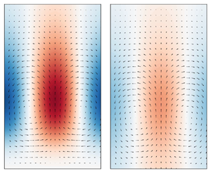
The effect of the non-diagonal components of the impedance tensor on the near-wall mode is further analysed by comparison of the predicted velocity fields with those of the uncontrolled flow for the resolvent mode resembling the near-wall cycle. Figure 7(a,b) shows the velocity fields of the near-wall mode for the uncontrolled flow in streamwise wall-normal $(x\unicode{x2013}y)$ and spanwise wall-normal $(z\unicode{x2013}y)$ planes. Note that the cross-sectional views in the $(z\unicode{x2013}y)$ planes for all cases are shown at the location where the streamwise velocity magnitude is maximum, which for the uncontrolled flow is shown by the dashed line in figure 7(a). The counter rotating streamwise vortices and the periodic ejections and sweeps commonly associated with the near-wall cycle are clearly seen in figure 7(a,b). Figures 7(c)–7(e) show the velocity structure in the $(z\unicode{x2013}y)$ plane for a favourable diagonal impedance tensor ($Z_{xx}=3+3{\rm i}$, $Z_{yy}=0.2+3{\rm i}$ shown by the $\circ$ symbol in figure 4) with different values of favourable $Z_{yx}$ and $Z_{xy}$. For $Z_{xy}=Z_{yx}=0$, figure 7(c), the wall impedance reduces the magnitude of wall-normal velocity compared with the uncontrolled flow. For the favourable non-diagonal impedances, $Z_{yx}=1+5{\rm i}$ (the $+$ symbol in figure 6b) and $Z_{xy}=1+1{\rm i}$ (the $+$ symbol in figure 6a), the wall-normal velocity magnitude is further reduced and the streamwise vortices are shifted further away from the wall. Furthermore, suctions and ejections at the wall in form of wall-normal velocity opposing the streamwise vortices are observed near the wall (figure 7d). Therefore favourable impedance tensors, either in diagonal or non-diagonal form, weaken the streamwise vortices and reduce the magnitude of peak wall-normal velocity.

Figure 7.

Velocity structure for near-wall mode: (a) streamwise velocity amplitude in the streamwise wall-normal plane for uncontrolled flow, (b–e) wall-normal and spanwise velocity fields in the spanwise wall-normal plane. The dashed line in (a) shows the streamwise location where the magnitude of streamwise velocity is maximum and the cross-sections for (b–e) are made. (a,b) Uncontrolled flow, (c) $Z_{yx}=Z_{xy}=0$, (d) $Z_{yx}=1+5{\rm i}$ and $Z_{xy}=0$, (e) $Z_{xy}=1+1{\rm i}$ and $Z_{yx}=0$ ($Z_{xx}=3+3{\rm i}, Z_{yy}=0.2+3{\rm i}$). The horizontal dotted line in (b–e) shows the centreline of the streamwise vortices.

The results presented in this section show the possibility of suppressing the near-wall cycle using frequency-tuned walls that permit transpiration and/or slip at the wall with a more reactive impedance. As the near-wall cycle is dynamically dominant at low Reynolds numbers, the results thus far suggest the potential of wall impedance in control of turbulent flows at the low Reynolds numbers. While the wall impedance must be within a favourable range (figures 4, 6), as shown by the results, the obtained gain and Reynolds stress reduction are not sensitive to the variations of impedance amplitude within the favourable range.

3.2. Effect of wall impedance on VLSMs

The effect of wall impedance on the modes resembling the VLSMs is considered in this section. Based on previous studies (McKeon & Sharma Reference McKeon and Sharma2010), the wavenumber–speed combination of $\boldsymbol {k}=(\kappa _{x}, \kappa _{z}, c^+)=(1,\pm 10,16)$ corresponding to $\lambda _{x}^+ \approx 6 h^+$ and $\lambda _{z}^+ \approx 0.6 h^+$ is selected to represent the VLSMs. Similar to the previous section, first a wall impedance with only diagonal components is considered and the mode gain and Reynolds stress contribution are estimated for a range of $Z_{xx}$ and $Z_{yy}$ values. Figure 8(a) shows the ratios of channel-integrated Reynolds shear stress for a sweep over $Z_{xx}$. For ${\rm Re}(Z_{xx}) \approx {\rm Im}(Z_{xx}) \geqslant 0.3$, $RS_{kc}/RS_{k0} \approx 1$ while for ${\rm Re}(Z_{xx}) \approx {\rm Im}(Z_{xx}) <10^{-1}$, the resolvent mode is amplified and $RS_{kc}$ increases. No regions of reduction in $\sigma _{kc}$ and $RS_{kc}$ are identified for a sweep over $Z_{xx}$ when $Z_{yy}=0$. As shown in figure 8(b), wall impedance with ${\rm Re}(Z_{yy}) \approx {\rm Im}(Z_{yy})<0.2$ creates a reduction in $RS_{kc}$ with approximately 64 % reduction in Reynolds stress contribution ($RS_{kc}/RS_{k0}=0.36$). Similar to the near-wall mode, the achievable reductions in the Reynolds shear stress contribution of the VLSM mode are not sensitive to the value of $Z_{yy}$ within its favourable range. When the non-diagonal components of the impedance tensor are considered, it is shown that, if the diagonal components are in the unfavourable range (the red zones of figure 8), the gain and Reynolds stress contribution ratios remain larger than 1 for any values of the non-diagonal components (similar to the observed effect on the near-wall modes). Similarly, for a favourable diagonal impedance tensor, the VLSM mode is found to be insensitive to variations of $Z_{xy}$ and $Z_{yx}$.

Figure 8.

Contour maps showing the ratio of control to uncontrolled flow channel-integrated Reynolds stress $RS_{kc}/RS_{k0}$ for the resolvent modes resembling VLSMs over a range of (a) $Z_{xx}$ ($Z_{yy}=0$) and (b) $Z_{yy}$ values ($Z_{xx}=0$) for a diagonal impedance tensor ($Z_{xy}=Z_{yx}=0$). The $+$ and $\circ$ symbols show the favourable and unfavourable cases referred to in figure 9.

Figure 9 shows the wall-normal profiles of the velocity and pressure fields, and figure 10 shows the velocity structure in the wall-normal spanwise plane for the mode resembling the VLSMs for the uncontrolled flow and the controlled cases with diagonal wall impedance. The velocity structure for the uncontrolled flow represents the characteristics of VLSMs consistent with previous studies showing periodic velocity fields with large streamwise roll cells (figure 10a). As shown by the wall-normal profiles of the uncontrolled flow, the pressure and wall-normal velocity fields have a constant phase with $y$ and a constant phase difference of ${\approx }{\rm \pi} /2$. Also, $v$ and $p$ have non-zero values at higher $y^+$ locations as compared with $u$ that fades to zero at $y^+=400$. Furthermore, the phase of the streamwise velocity decreases with $y$ showing the mode inclination in downstream direction. This mode actively contributes to the Reynolds stress mainly at the critical layer location where streamwise and wall-normal velocities are ${\approx }{\rm \pi}$ out of phase.

Figure 9.

Profiles showing the wall-normal variation in structure for the resolvent mode resembling VLSMs: (a,d,g) amplitude and (b,e,h) phase for the streamwise velocity (solid lines), wall-normal velocity (dashed lines) and pressure fields (dotted lines); (c, f,i) the normalised Reynolds stress contribution. (a–c) Represent the uncontrolled flow (the impermeable wall), (d–f) represent a favourable diagonal wall impedance ($Z_{yy}=0.03+0.03$i, $Z_{xx}=Z_{xy}=Z_{yx}=0$) and (g–i) represent an unfavourable diagonal wall impedance ($Z_{yy}=0.3+0.8$i, $Z_{xx}=0.1+0.1$i, $Z_{xy}=Z_{yx}=0$). The dotted horizontal lines show the location of the critical layer for this mode at $y^+ \approx 95$.

Figure 10.

Wall-normal and spanwise velocity fields in the spanwise wall-normal plane for VLSM mode: (a) uncontrolled flow, (b) favourable diagonal impedance ($Z_{yy}=0.03+0.03$i, $Z_{xx}=Z_{xy}=Z_{yx}=0$), (c) unfavourable diagonal impedance ($Z_{yy}=0.3+0.8$i, $Z_{xx}=0.1+0.1$i, $Z_{xy}=Z_{yx}=0$).

For a favourable drag-reducing pressure-driven diagonal impedance tensor (figure 9d–f), the peak of the wall-normal and streamwise velocity components and the streamwise velocity gradient near the wall are significantly reduced. The phase difference between wall-normal velocity and pressure fields is reduced at and slightly below the critical layer. These changes lead to a significant reduction in the peak of Reynolds stress and changes in its profile below the critical layer. A non-zero wall-normal velocity in form of blowing/suction exists at the wall and the rollers are suppressed (figure 10b). These observations show that the favourable wall impedance weakens the streamwise roll cells through admitting wall transpiration.

For the unfavourable diagonal impedance, figure 9(g–i), the streamwise and wall-normal velocity fields near the wall are altered, admitting both transpiration and slip at the wall. The slip and transpiration at the wall and the change in phase difference between $u$ and $v$ create a non-zero Reynolds stress at the wall (figure 9i). In this case, the rollers are shifted closer to the wall (figure 10c). Despite the reduction in peak wall-normal velocity, the concentration of peak Reynolds stress at the critical layer and near the wall and the largely increased mode gain lead to an overall increase of channel-integrated Reynolds stress for this case.

3.3. Effect of wall impedance in the spectral space

In the previous sections, the effects of wall impedance on individual resolvent modes that resemble the coherent structures of dynamic importance have been discussed. However, to evaluate the overall efficiency of wall impedance as a control method, it is necessary to consider its effects on the other modes in the spectral space and with different propagation speeds. For this investigation, two sample impedance tensors, which have been identified as favourable drag-reducing cases, for the near-wall and VLSM modes in the previous sections, are considered. Figure 11 shows the effect of the wall impedance tensors on the gain ratio of other modes as functions of streamwise wavenumber $\kappa _{x}$ and mode speed $c^+$ at $\kappa _{z}=0$, $\kappa _{z}=10$ and $\kappa _{z}=120$. The propagation speed is considered in the range of $\approx 0.1U^+_{CL} - 1.0U^+_{CL}$ as the structures with speeds larger than the channel centreline velocity are known to have negligible energy contributions in real turbulent flows (McKeon Reference McKeon2017). Note that for modes with identical wavelengths, faster-moving modes with a higher propagation speed are located further away from the wall as compared with the slower-moving modes (McKeon & Sharma Reference McKeon and Sharma2010). Hence, the slower-moving modes have a larger wall-pressure signature. With increase of mode speed, the structure moves further away from the wall and its wall-pressure signature reduces. Above a wavelength-dependent threshold speed, the modes become detached with a nearly zero wall-pressure signature. Modes with a larger wavelength become detached at higher propagation speeds as they have a larger wall-normal extent (McKeon Reference McKeon2017).

Figure 11.

Contour maps showing the singular value ratios $\sigma _{kc}/\sigma _{k0}$ as a function of streamwise wavenumber $\kappa _{x}$ and mode speed $c^+$ at (a,d) $\kappa _{z}=0$ (spanwise constant), (b,e) $\kappa _{z}=10$ ($\lambda _{z}^+ \approx 0.6 h^+$) and (c, f) $\kappa _{z}=120$ ($\lambda _{z}^+\approx 10^2$). (a–c) Correspond to a favourable impedance tensor for the near-wall cycle ($Z_{xx}=3+3$i, $Z_{yy}=0.2+3$i, $Z_{xy}=Z_{yx}=0$) and (d–f) correspond to a favourable impedance tensor for the VLSMs ($Z_{xx}=0.01+0.01$i, $Z_{yy}=0.03+0.03$i, $Z_{xy}=Z_{yx}=0$). The $+$ symbol shows the VLSM mode $(\kappa _{x}, \kappa _{z})=(1,10)$, and the $\circ$ represents the near-wall cycle $(\kappa _{x}, \kappa _{z})=(10,120)$.

Figure 11(a–c) corresponds to a wall impedance tensor which suppresses the near-wall mode ($Z_{xx}=3+3$i, $Z_{yy}=0.2+3$i, $Z_{xy}=Z_{yx}=0$). Figure 11(a) shows that the favourable impedance for the near-wall mode suppresses the spanwise-constant attached slower-moving modes ($\kappa _{z}=0, \kappa _{x}>1$, and $c^+<18$) while amplifying large faster-moving modes ($\kappa _{x} \approx 0.1$ and $c^+>18$). It is noteworthy that, at the considered Reynolds number, these modes have lower gain values and, therefore, the negative effect on these modes will make an almost negligible contribution to the total drag. At $\kappa _{z}=10$, figure 11(b), slower-moving modes with $\kappa _{x}>10$ and $\kappa _{x}<1$ are suppressed, while other modes are slightly amplified or unchanged, including the VLSM mode which is slightly amplified with a sigma ratio of 1.2. For $\kappa _{z}=120$, figure 11(c), the wall impedance reduces the gain ratio of shorter faster-moving modes ($\kappa _{x}>10$ and $c^+<15$) and has negligible effect on other modes. For the specific wavenumber–frequency combination of $(\kappa _{x}, \kappa _{z})=(10,120)$, slower-moving modes with $c^+ \leqslant 10$ are classified as attached to the wall, and as the propagation speed increases the modes become detached and the peak of wall-normal velocity moves further away from the wall located at the critical layer (Luhar, Sharma & McKeon Reference Luhar, Sharma and McKeon2014a). Therefore, the gain ratios in figure 11(c) show that a wall impedance favourable for the near-wall mode suppresses the attached modes while having no significant effect on detached modes far from the wall.

Figure 11(d–f) shows the effect of a wall impedance which favourably suppresses the VLSMs ($Z_{xx}=0.01+0.01$i, $Z_{yy}=0.03+0.03$i, $Z_{xy}=Z_{yx}=0$) in the spectral space. For both spanwise-constant modes and $\kappa _{z}=10$, it suppresses energetic structures at $0.2<\kappa _{x}<2$ and $c^+\approx 15$, while either having no significant effect on or amplifying the other modes. This impedance is found to significantly amplify detached spanwise-constant large-scale structures at $0.1<\kappa _{x}<3$ (figure 11d). At $\kappa _{z}=10$ and $\kappa _{z}=120$, the wall impedance amplifies large-scale structures with $\kappa _{x}<1$ and $\kappa _{x}<10$, respectively. Note that, while these results are presented for diagonal impedance tensors, similar effects in the spectral space were found for non-diagonal tensors. The spectral analysis in this section therefore suggests that a wall impedance tensor that can favourably suppress the near-wall modes also weakens a large range of other wavenumbers and is therefore more likely to have an overall drag-reducing effect than a wall that is targeted at suppression of VLSMs.

4. Shear-driven vs pressure-driven impedance

The analysis using the impedance tensor in the previous sections considered both wall-shear- and pressure-driven impedances, and identified the combinations of $Z_{xx}$ and $Z_{yy}$ which could favourably suppress the dynamically important turbulent structures. As discussed in § 1, control of turbulent flow by application of passive walls driven by wall shear stress has been explored in the literature (Fukagata et al. Reference Fukagata, Kern, Chatelain, Koumoutsakos and Kasagi2008; Józsa et al. Reference Józsa, Balaras, Kashtalyan, Borthwick and Viola2019). However, per the authors’ knowledge, a comparison of the efficiency of these two approaches for passive control is not available. Hence, the developed model in this study is used to compare the control approaches based on wall-shear- and pressure-driven impedances by considering wall impedance tensors with non-zero components for only $Z_{xx}$ and $Z_{yy}$, respectively. Note that the shear-driven impedance permits only slip, while the pressure-driven impedance allows only transpiration at the wall.

Independent parameter sweeps are conducted for wall impedance tensors with non-zero components for only $Z_{xx}$ and $Z_{yy}$ and the gains of the modes resembling the near-wall cycle and the VLSMs are evaluated. Based on these parameter sweeps, two sample impedance tensors are considered and the efficiency of the control in the spectral space and at different propagation speeds is evaluated. For this analysis, it is assumed that there is unit forcing over the range of wave speeds $0< c^+< U^+_{CL}$ and the effect of the wall impedance in the spectral space $10^{-1}< (\kappa _{x},\kappa _{z}) <10^2$ is estimated by integrating the mode gains over the range of wave speeds, i.e.

(4.1)

\begin{equation} \tilde{\sigma}(\kappa_{x},\kappa_{z})=\int \sigma(\kappa_{x},\kappa_{z},c^+) \,\mathrm{d}c^+. \end{equation}

Figure 12 shows the ratio of the integrated mode gain for the controlled flow to the uncontrolled flow, $\tilde {\sigma }_{kc} / \tilde {\sigma }_{k0}$, over a range of $(\kappa _{x},\kappa _{z})$ for streamwise-shear-driven ($Z_{xx}$ only) and pressure-driven ($Z_{yy}$ only) controls. The shear-driven control, figure 12(a), which only permits slip at the wall, has a gain-reducing effect over a large region in the spectral domain and slightly reduces the mode gain compared with the uncontrolled flow ($\tilde {\sigma }_{kc} / \tilde {\sigma }_{k0} >0.9$).

Figure 12.

Contour maps showing the normalised integrated singular value ratios $\tilde {\sigma }_{kc} / \tilde {\sigma }_{k0}$ as a function of streamwise wavenumber $\kappa _{x}$ and spanwise wavenumber $\kappa _{z}$ for (a) shear-driven control ($Z_{xx}=0.5+0.5$i, $Z_{yy}=Z_{xy}=Z_{yx}=0$), and (b) pressure-driven control ($Z_{yy}=0.2+3$i, $Z_{xx}=Z_{xy}=Z_{yx}=0$). The $+$ symbol shows the VLSM mode $(\kappa _{x}, \kappa _{z})=(1,10)$, and the $\circ$ represents the near-wall cycle $(\kappa _{x}, \kappa _{z})=(10,120)$.

Figure 12(b) shows that a pressure-driven control ($Z_{yy}$ only) permitting only transpiration at the wall leads to gain reduction or no significant effect over a large range of the wavenumbers including both the near-wall and VLSM modes, while having a detrimental effect on other wavenumbers and slightly amplifying spanwise modes ($\kappa _{z} \approx 1$) and modes at $\kappa _{x} \approx 100$. Hence, the predictions of the present resolvent analysis suggest that a surface with a shear-driven wall impedance can more effectively suppress a range of resolvent modes and thus lead to likely turbulent drag reduction compared with a surface with pressure-driven impedance.

5. Effect of Reynolds number on control performance

The results of this study, which thus far were presented for a turbulent channel flow at $\textit {Re}_{\tau }=2000$, show that different impedance characteristics are required to suppress VLSMs and near-wall modes. To further explore the effect of Reynolds number on efficiency of wall impedance as a control strategy, the resolvent modes are calculated for $\textit {Re}_{\tau }=2 \times 10^4$. Figure 13 shows the effect of Reynolds number on the normalised integrated singular value ratios (calculated from (4.1) over the range of wave speeds $0< c^+< U^+_{CL}$ and wavenumbers $10^{-1}< (\kappa _{x},\kappa _{z}) <10^2$) for three impedance tensors. First, a diagonal impedance tensor, which was determined as favourable for VLSM modes in the previous sections, is considered and the integrated singular value ratios are shown for $\textit {Re}_{\tau }=2000$ and $\textit {Re}_{\tau }=2 \times 10^4$ (figure 13a,b). With an increase of Reynolds number, the same surface impedance suppresses a similar range of large-scale structures that were suppressed at the lower Reynolds number. On the other hand, large streamwise structures with $0.1<\kappa _{x}<1$ and $1<\kappa _{z}<10^2$ are amplified at the higher Reynolds number. The effect of increase of Reynolds number on control performance is next investigated for the shear-driven only and pressure-driven only wall impedances, (see figure 12 at $\textit {Re}_{\tau }=2000$ and figures 13(c) and 13(d) at $\textit {Re}_{\tau }=2 \times 10^4$). Similar to the results at the lower Reynolds number, the shear-driven impedance suppresses a large range of modes and has a negligible impact on the rest, with an overall drag-reducing effect. For the pressure-driven impedance (figure 13d), the control performance improves with the increase of Reynolds number. At the higher Reynolds number, resolvent modes with $1<\kappa _{x}<10$ and $1<\kappa _{z}<30$ which were amplified at $\textit {Re}_{\tau }=2000$ are suppressed (see figures 12b and 13d), and the overall Reynolds stress contribution integrated over the spectral domain is decreased compared with the uncontrolled flow by 2 %. The results therefore show that, for the considered pressure-driven only impedance, the drag-reducing performance improves with the increase of Reynolds number.

Figure 13.

Contour maps showing the normalised integrated singular value ratios $\tilde {\sigma }_{kc} / \tilde {\sigma }_{k0}$ as a function of streamwise wavenumber $\kappa _{x}$ and spanwise wavenumber $\kappa _{z}$ for: a pressure- and shear-driven diagonal impedance ($Z_{xx}=0.01+0.01$i, $Z_{yy}=0.03+0.03$i, $Z_{xy}=Z_{yx}=0$) at (a) $\textit {Re}_{\tau }=2000$ and (b) $\textit {Re}_{\tau }=2 \times 10^4$ and (c) shear-driven impedance at $\textit {Re}_{\tau }=2 \times 10^4$ ($Z_{xx}=0.5+0.5$i, $Z_{yy}=Z_{xy}=Z_{yx}=0$) and (d) pressure-driven impedance at $\textit {Re}_{\tau }=2 \times 10^4$ ($Z_{yy}=0.2+3$i, $Z_{xx}=Z_{xy}=Z_{yx}=0$). The $+$ symbol shows the VLSM mode $(\kappa _{x}, \kappa _{z})=(1,10)$, and the $\circ$ represents the near-wall cycle $(\kappa _{x}, \kappa _{z})=(10,120)$.

6. Implications for design of frequency-tuned walls

The developed model using resolvent analysis shows a potential for passive control of wall-bounded turbulence using impedance surfaces that permit transpiration and/or slip. The estimations of the gain reductions achieved for the near-wall and VLSMs using the impedance walls are comparable to those for compliant walls by Luhar et al. (Reference Luhar, Sharma and McKeon2015). The favourable wall impedance was found to create a maximum gain reduction of 15 % for the near-wall mode and 23 % for the VLSMs. Quite similarly, the optimum compliant wall was found to reduce the near-wall and VLSM mode gains by 32 % and 48 %, respectively (Luhar et al. Reference Luhar, Sharma and McKeon2015). A key finding that distinguishes the impedance walls from compliant walls is that the favourable surface impedance is non-unique. Lack of sensitivity of the control performance to small variations of wall impedance is an important advantage that benefits the design of frequency-tuned surfaces. The non-uniqueness of the favourable surface impedance also implies that ordered material design can be employed to target certain frequency bandwidths and wavenumber regimes.

Using the bulk impedance boundary condition for the wall, instead of directly modelling a specific geometry, the findings of this study provide insights into design of geometries that permit or reject slip and/or transpiration for specific periodicity. Examples of surfaces that can create the desired impedance are porous and perforated surfaces. These surfaces are non-deformable (in contrast to compliant surfaces) and their interaction with the flow can be described using the wall impedance boundary condition as the porosity of the surface allows some absorption of flow perturbations. Some applications of these surfaces have been explored in the literature, as discussed in § 1, including porous surfaces with subsurface chambers (that permit wall transpiration) for control of transition (Porter Reference Porter1998) and turbulent boundary layers (Silvestri et al. Reference Silvestri, Ghanadi, Arjomandi, Cazzolato and Zander2017; Jafari et al. Reference Jafari, Cazzolato and Arjomandi2022). It is possible to create the desired impedance by varying the geometric parameters of the perforated surfaces. As determined through classic acoustic approaches, the real component of $Z_{yy}$ is mainly a function of the dimensions of the perforations, while the volume of subsurface chamber mainly affects the imaginary component. Per authors’ knowledge, experimental measurement of $Z_{xx}$ for perforated surfaces is not available in the literature. However, estimations can be made from impedance measurements in the presence of grazing shear flow. For example, Schulz et al. (Reference Schulz, Weng, Bake, Enghardt and Ronneberger2017) conducted impedance measurements of acoustic liners made of perforated sheets (with circular perforations of 1–2 mm in diameter and 0.5–2 mm in depth) with a backing structure consisting of individual cells (6.9 mm in diameter and 40 mm in depth) in a flow duct facility (DUCT-R52 of the German Aerospace Centre) over a range of flow speeds in the range $10\unicode{x2013}105\ {\rm m}\ {\rm s}^{-1}$. It was found that, for these perforated surfaces: $1<{\rm Re}(Z_{yy})/ \rho c<5$ and $0<{\rm Im}(Z_{yy})/\rho c<5$, and $0.02<{\rm Re}(Z_{T})/ \rho c<0.1$ and $-0.6<{\rm Im}(Z_{T})/ \rho c<0.4$ over the range of frequencies between 300 and 2000 Hz. Here, $\rho$ and $c$ are the fluid density and speed of sound, and $Z_{T}=- \tau _{xy} /v$ represents the wall-shear-driven impedance (although not identical to $Z_{xx}$ in definition). Based on the estimations of impedance for the perforated surfaces, such surfaces are a potential candidate for passive control and are subject of ongoing work by the authors. Furthermore, with advances in the additive manufacturing techniques, it is possible to design and fabricate other geometries with desired impedances for specific periodicity for the control of wall turbulence.

7. Conclusions

The potential of frequency-tuned surfaces for passive control of wall-bounded turbulent flows was investigated in this study. Using a generalised impedance wall-boundary condition, surfaces that permit slip and/or transpiration in response to wall pressure and/or shear were explored. The conducted analysis showed that the surface impedance is non-unique, meaning certain wavenumber regimes can be targeted by periodic material design. These surfaces can be designed in form of metamaterials using additive manufacturing techniques to favourably target energetic turbulent structures through wall impedance. The control performance is not sensitive to variations in the amplitude of wall impedance as long as it is within a favourable range. This is an advantage that makes the application of wall impedance for passive control promising.

The predictions made by resolvent analysis show that an impedance wall can suppress the dynamically important structures of the wall-bounded turbulent flows, namely, the near-wall cycle and the VLSMs, and thereby reduce the turbulent component of friction drag. It is shown that the effect of impedance mainly depends on the diagonal components of the impedance tensor, i.e. $Z_{xx}$ and $Z_{yy}$. Suppression of the near-wall cycle requires a more reactive impedance compared with that required for suppression of VLSMs. Non-diagonal impedance tensors with $Z_{xy}$ and $Z_{yx}$ values smaller than certain thresholds suppress the near-wall and VLSM modes. For impedances considering both shear- and pressure- driven impedance components, the favourable impedance for suppression of both modes is found to permit transpiration and reject slip. For the near-wall cycle, walls that lead to reduced phase difference between pressure and streamwise velocity at the wall amplify the near-wall mode, while impedances that lead to reduced phase difference between pressure and wall-normal velocity at the wall are favourable for mode suppression. The latter was also reported by Luhar et al. (Reference Luhar, Sharma and McKeon2015) for a compliant wall that suppresses the near-wall cycle. Analysis of the effect of wall impedance on modes with varying speeds and wavelengths showed that a wall impedance that favourably suppresses the near-wall modes also weakens a large range of modes in the spectral space. Therefore, materials with an impedance that targets the near-wall cycle will also more effectively suppress other scales and will likely have an overall drag reducing effect. This is in contrast to compliant walls for which a wall optimised for suppression of the near-wall cycle is found to have a smaller reach in spectral space compared with the wall optimised for the VLSM modes (Luhar et al. Reference Luhar, Sharma and McKeon2015). Using the developed impedance model, passive control based on only pressure-driven impedance and only shear-driven impedance were compared. It is shown that a wall with streamwise-shear-driven impedance can lead to suppression of turbulent structures over a wide range in spectral space, while pressure-driven impedance has a more inconsistent spectral footprint.

There are assumptions in the presents analysis which must be kept in mind. It has been assumed that the wall can support a given impedance with a geometry that can support transpiration and/or slip. Furthermore, the bulk impedance approach does not consider the likely effect of surface length scales (such as the spacing of perforations in the case of a porous surface). In this study, the gain and structure of resolvent modes are analysed. While the reduction of mode gain indicates suppression of modes and reduction of Reynolds stress contribution of modes, it does not directly predict the effects of wall impedance on skin friction or the mean velocity profile. A more complete model would need to consider the nonlinear interactions between the modes. Furthermore, the present results were obtained using a canonical mean velocity profile (which may vary in the modified flow). The application of the canonical velocity profile may affect the predicted drag reduction trends if there is a substantial modification in the controlled mean velocity profile, due to for example large-scale changes of flow structure. However, it is shown to provide a sufficient estimation for analysis of the response of the nonlinear system to control (Toedtli et al. Reference Toedtli, Luhar and McKeon2019). Despite the discussed limitations, it has been previously shown that resolvent analysis can act as a computationally inexpensive method for design and first-order test of control strategies. The present study using the bulk impedance approach shows a potential for passive control using material impedance. The next step would be design of (meta)materials that could create the desired impedances and realisation of the predictions of this analysis using experimental and numerical modellings.

Funding

This work was supported by the Australian Research Council Discovery Projects (grant number DP200101961); and the U.S. Office of Naval Research (grant number N00014-17-1-3022, BJM).

Declaration of interests

The authors report no conflict of interest.

Appendix. Rank-1 approximation

In the present study, the effect of wall impedance on the turbulent flow was investigated by considering the rank-1 approximation of the resolvent. Although it has been shown that rank-1 approximation can represent the characteristics of the most energetic modes of wall-bounded turbulence (Moarref et al. Reference Moarref, Sharma, Tropp and McKeon2013), the reconstruction of the full field and energy spectra requires higher rank modes, with approximately 10 ranks providing a good representation of the experimentally observed structures and velocity spectra (McKeon Reference McKeon2017). In this appendix, we show that the rank-1 approximation provides a sufficient estimation for suppression of modes and turbulent drag reduction.

Two sample impedance tensors, which have been identified as favourable for suppression of the near-wall and VLSM modes from the rank-1 approximation, are selected. Figure 14 shows the gain, $\sigma _{k,m}$, of near-wall and VLSM modes for the uncontrolled flow and the impedance walls for up to $m=20$. Note that almost all resolvent modes are paired (i.e. $\sigma _{k,1}=\sigma _{k,2}$, $\sigma _{k,3}=\sigma _{k,4}$, and so on) such that each two modes in a pair are symmetric/anti-symmetric counterparts of each other with the same magnitude. As shown in figure 14, the favourable impedances reduce the mode gain for rank-1 and rank-2 substantially, while the gains of higher ranks ($m=3\unicode{x2013}8$) increase slightly. As the first mode pair have the largest gain, they make the largest contribution to the total response assuming broadband forcing. In addition, the increase in mode gain for higher ranks due to the wall impedance can be considered negligible compared with the achieved gain reduction for $\sigma _{k,1}$ and $\sigma _{k,2}$. Hence, the gain reduction of rank-1 leads to an overall turbulent drag reduction. This is supported by the calculated Reynolds stress contribution of the modes. The channel-integrated Reynolds stress contribution is calculated by considering 20 modes, i.e. $\sum _{m=1}^{20} \int _{0}^{2} \sigma _{k,m}^2 \,Re(u_{k,m}^{*} v_{k,m}) (y-1) \,\mathrm {d}y$. It is found that the wall impedance reduces the Reynolds stress contribution, accounting for 20 ranks, by 48 % for the near-wall mode, and by 40 % for the VLSM mode. If only the rank-1 approximation is considered, the reduction in Reynolds stress contribution changes to 33 % and 29 % for the near-wall and VLSM modes, respectively. Hence, a sufficient approximation of the control performance is provided by considering only rank 1. Note that, although rank-1 and rank-2 almost equally contribute to the total flow response (as $\sigma _{k,1}=\sigma _{k,2}$), because they are the symmetric/anti-symmetric counterparts of a pair, the control impact can be sufficiently described by accounting for only rank 1, and considering both of them will yield the same result.

Figure 14.

Singular values for high ranks up to $m=20$ for the resolvent mode representing: (a) the near-wall cycle, (b) VLSMs. The black solid line shows the uncontrolled flow and the blue dashed line shows an impedance wall favourable for suppression of the near-wall mode in (a), ($Z_{xx}=3+3$i, $Z_{yy}=0.2+3$i, $Z_{xy}=Z_{yx}=0$) and favourable for suppression of the VLSMs in (b) ($Z_{yy}=0.03+0.03$i, $Z_{xx}=Z_{xy}=Z_{yx}=0$).

References

REFERENCES

Bhat, S.S., Silvestri, A., Cazzolato, B. & Arjomandi, M. 2021 Mechanism of control of the near-wall turbulence using a micro-cavity array. Phys. Fluids 33, 075114.CrossRef Google Scholar

Boden, H., Cordioli, J.A., Spillere, A. & Serrano, P. 2017 Comparison of the effect of flow direction on liner impedance using different measurement methods. In 23rd AIAA/CEAS Aeroacoustics Conference. American Institute of Aeronautics and Astronautics.CrossRef Google Scholar

Breugem, W.P., Boersma, B.J. & Uittenbogaard, R.E. 2006 The influence of wall permeability on turbulent channel flow. J. Fluid Mech. 562, 35.CrossRef Google Scholar

Burden, H.W. 1969 The effect of wall porosity on the stability of parallel flows over compliant boundaries. PhD thesis, University of Pennsylvania.Google Scholar

Chavarin, A., Efstathiou, C., Vijay, S. & Luhar, M. 2020 Resolvent-based design and experimental testing of porous materials for passive turbulence control. Intl J. Heat Fluid Flow 86, 108722.CrossRef Google Scholar

Chavarin, A., de Segura, G.G., García-Mayoral, R. & Luhar, M. 2021 Resolvent-based predictions for turbulent flow over anisotropic permeable substrates. J. Fluid Mech. 913, A24.CrossRef Google Scholar

Dai, X. & Auregan, Y. 2016 Influence of shear flow on liner impedance computed by multimodal method. In 22nd AIAA/CEAS Aeroacoustics Conference. American Institute of Aeronautics and Astronautics.CrossRef Google Scholar

Fukagata, K., Kern, S., Chatelain, P., Koumoutsakos, P. & Kasagi, N. 2008 Evolutionary optimization of an anisotropic compliant surface for turbulent friction drag reduction. J. Turbul. 9, N35.CrossRef Google Scholar

Gabard, G. 2020 Generalised acoustic impedance for viscous fluids. J. Sound Vib. 484, 115525.CrossRef Google Scholar

Gad-el-Hak, M. 1994 Interactive control of turbulent boundary layers – a futuristic overview. AIAA J. 32 (9), 1753–1765.CrossRef Google Scholar

Jafari, A., Cazzolato, B. & Arjomandi, M. 2022 Finite-length porous surfaces for control of a turbulent boundary layer. Phys. Fluids 34 (4), 045115.CrossRef Google Scholar

Jiménez, J., Uhlmann, M., Pinelli, A. & Kawahara, G. 2001 Turbulent shear flow over active and passive porous surfaces. J. Fluid Mech. 442, 89–117.CrossRef Google Scholar

Józsa, T.I., Balaras, E., Kashtalyan, M., Borthwick, A.G.L. & Viola, I.M. 2019 Active and passive in-plane wall fluctuations in turbulent channel flows. J. Fluid Mech. 866, 689–720.CrossRef Google Scholar

Kim, E. & Choi, H. 2014 Space–time characteristics of a compliant wall in a turbulent channel flow. J. Fluid Mech. 756, 30–53.CrossRef Google Scholar

Kuwata, Y. & Suga, K. 2017 Direct numerical simulation of turbulence over anisotropic porous media. J. Fluid Mech. 831, 41–71.CrossRef Google Scholar

Landahl, M.T. 1962 On the stability of a laminar incompressible boundary layer over a flexible surface. J. Fluid Mech. 13 (4), 609–632.CrossRef Google Scholar

Lee, T., Fisher, M. & Schwarz, W.H. 1993 Investigation of the stable interaction of a passive compliant surface with a turbulent boundary layer. J. Fluid Mech. 257, 373–401.CrossRef Google Scholar

Luhar, M., Sharma, A.S. & McKeon, B.J. 2014 a On the structure and origin of pressure fluctuations in wall turbulence: predictions based on the resolvent analysis. J. Fluid Mech. 751, 38–70.CrossRef Google Scholar

Luhar, M., Sharma, A.S. & McKeon, B.J. 2014 b Opposition control within the resolvent analysis framework. J. Fluid Mech. 749, 597–626.CrossRef Google Scholar

Luhar, M., Sharma, A.S. & McKeon, B.J. 2015 A framework for studying the effect of compliant surfaces on wall turbulence. J. Fluid Mech. 768, 415–441.CrossRef Google Scholar

Luhar, M., Sharma, A.S. & McKeon, B.J. 2016 On the design of optimal compliant walls for turbulence control. J. Turbul. 17 (8), 787–806.CrossRef Google Scholar

Mathis, R., Hutchins, N. & Marusic, I. 2009 Large-scale amplitude modulation of the small-scale structures in turbulent boundary layers. J. Fluid Mech. 628, 311–337.Google Scholar

McKeon, B.J. 2017 The engine behind (wall) turbulence: perspectives on scale interactions. J. Fluid Mech. 817, P1.CrossRef Google Scholar

McKeon, B.J. & Sharma, A.S. 2010 A critical-layer framework for turbulent pipe flow. J. Fluid Mech. 658, 336–382.CrossRef Google Scholar

McKeon, B.J., Sharma, A.S. & Jacobi, I. 2013 Experimental manipulation of wall turbulence: a systems approach. Phys. Fluids 25 (3), 031301.CrossRef Google Scholar

Moarref, R., Sharma, A.S., Tropp, J.A. & McKeon, B.J. 2013 Model-based scaling of the streamwise energy density in high-Reynolds-number turbulent channels. J. Fluid Mech. 734, 275–316.CrossRef Google Scholar

Nagy, P.T. & Paál, G. 2019 Stabilization of the boundary layer by streamwise control. Phys. Fluids 31 (12), 124107.CrossRef Google Scholar

Nakashima, S., Fukagata, K. & Luhar, M. 2017 Assessment of suboptimal control for turbulent skin friction reduction via resolvent analysis. J. Fluid Mech. 828, 496–526.CrossRef Google Scholar

Porter, L.J. 1998 The effects of passive wall porosity on the linear stability of boundary layers. PhD thesis, University of Warwick.Google Scholar

Renou, Y. & Aurégan, Y. 2011 Failure of the Ingard–Myers boundary condition for a lined duct: an experimental investigation. J. Acoust. Soc. Am. 130 (1), 52–60.CrossRef Google Scholar PubMed

Reynolds, W.C. & Tiederman, W.G. 1967 Stability of turbulent channel flow, with application to Malkus's theory. J. Fluid Mech. 27 (2), 253–272.CrossRef Google Scholar

Schulz, A., Weng, C., Bake, F., Enghardt, L. & Ronneberger, D. 2017 Modeling of liner impedance with grazing shear flow using a new momentum transfer boundary condition. In 23rd AIAA/CEAS Aeroacoustics Conference. American Institute of Aeronautics and Astronautics.CrossRef Google Scholar

Sharma, A.S. & McKeon, B.J. 2013 On coherent structure in wall turbulence. J. Fluid Mech. 728, 196–238.CrossRef Google Scholar

Silvestri, A., Ghanadi, F., Arjomandi, M., Cazzolato, B. & Zander, A. 2017 Attenuation of sweep events in a turbulent boundary layer using micro-cavities. Exp. Fluids 58, 58.CrossRef Google Scholar

Smits, A.J., McKeon, B.J. & Marusic, I. 2011 High–Reynolds number wall turbulence. Annu. Rev. Fluid Mech. 43 (1), 353–375.CrossRef Google Scholar

Suga, K., Okazaki, Y., Ho, U. & Kuwata, Y. 2018 Anisotropic wall permeability effects on turbulent channel flows. J. Fluid Mech. 855, 983–1016.CrossRef Google Scholar

Toedtli, S.S., Luhar, M. & McKeon, B.J. 2019 Predicting the response of turbulent channel flow to varying-phase opposition control: resolvent analysis as a tool for flow control design. Phys. Rev. Fluids 4 (7), 073905.CrossRef Google Scholar

Towne, A., Lozano-Durán, A. & Yang, X. 2019 Resolvent-based estimation of space–time flow statistics. J. Fluid Mech. 883, A17.CrossRef Google Scholar

Xia, Q.J., Huang, W.X. & Xu, C.X. 2017 Direct numerical simulation of turbulent boundary layer over a compliant wall. J. Fluids Struct. 71, 126–142.CrossRef Google Scholar

Xu, S., Rempfer, D. & Lumley, J. 2003 Turbulence over a compliant surface: numerical simulation and analysis. J. Fluid Mech. 478, 11–34.CrossRef Google Scholar

Figure 1.Resolvent analysis predictions for the passive streamwise-shear-driven impedance study by Józsa et al. (2019): (a) Reynolds shear stress profiles from DNS results by Józsa et al. (2019), and (b) Reynolds shear stress contribution of the resolvent mode representing the near-wall cycle. The black solid lines show the base flow and the dashed blue lines correspond to the control case. (c) The ratio of drag for control to base flow for different damping ratios obtained for the near-wall resolvent mode in comparison with total drag determined from DNS. The filled blue circles show the predictions by resolvent analysis and the unfilled black circles show the DNS results by Józsa et al. (2019).

Figure 2.Gain ratios for spanwise-constant modes ($\kappa _{z}=0$) over a range of streamwise wavenumbers and wave speeds for the passive pressure-driven compliant wall by Kim & Choi (2014) predicted by resolvent analysis: (a) considering only the wall impedance, and (b) considering both impedance and the wall motion. The $+$ symbol represents the two-dimensional waves observed in DNS of Kim & Choi (2014).

Figure 3.Resolvent analysis predictions for the porous wall of Jiménez et al. (2001): (a) ratio of porous to impermeable wall singular values $\sigma _{kc}/\sigma _{k0}$ for spanwise-constant resolvent modes for a range of streamwise wavenumbers and wave speeds at $\textit {Re}_{\tau }=180$; (b) wall-normal and streamwise velocity fields for the amplified mode at $(\kappa _{x},\kappa _{z},c^+) \approx (1.2,0,12.5)$. The $+$ symbol in (a) shows the wavenumber and speed of rollers identified in the DNS study by Jiménez et al. (2001).

Figure 4.Contour maps showing the ratio of control to uncontrolled flow singular values $\sigma _{kc}/\sigma _{k0}$ and channel-integrated Reynolds stress $RS_{kc}/RS_{k0}$ for the resolvent modes resembling the near-wall cycle over a range of $Z_{xx}$ and $Z_{yy}$ values for a diagonal impedance tensor ($Z_{xy}=Z_{yx}=0$). (a,b) Ratios of singular value and Reynolds stress for a sweep over $Z_{xx}$ at $Z_{yy}=0$, (c,d) ratios of singular value and Reynolds stress for a sweep over $Z_{yy}$ at $Z_{xx}=0$, (e) Reynolds stress ratios for a sweep over $Z_{xx}$ at $Z_{yy}=0.2+3$i (the $+$ symbol in c,d) and ( f) Reynolds stress ratios for a sweep over $Z_{yy}$ at $Z_{xx}=0.5+0.5{\rm i}$ (the $+$ symbol in a,b). The $\circ$ and $\times$ symbols in (e, f) show the favourable and unfavourable cases referred to in figure 5.

Figure 5.Profiles showing the wall-normal variation in structure for the resolvent mode resembling the near-wall cycle: (a,d,g) amplitude and (b,e,h) phase for the streamwise velocity (solid lines), wall-normal velocity (dashed lines) and pressure fields (dotted lines); (c, f,i) the normalised Reynolds stress contribution. (a–c) Represent the uncontrolled flow (the impermeable wall), (d–f) represent a favourable wall impedance ($Z_{xx}=3 +3{\rm i}$, $Z_{yy}=0.2+3{\rm i}$, $Z_{xy}=Z_{yx}=0$) and (g–i) represent an unfavourable wall impedance ($Z_{xx}=0.5+0.5{\rm i}$, $Z_{yy}=0.5+0.5{\rm i}$, $Z_{xy}=Z_{yx}=0$). The dotted horizontal lines show the location of the critical layer for this resolvent mode at $y^+ \approx 15$.

Figure 6.Contour maps showing the ratio of control to uncontrolled flow channel-integrated Reynolds stress $RS_{kc}/RS_{k0}$ for the resolvent modes resembling the near-wall cycle over a range of (a) $Z_{xy}$ values and $Z_{yx}=0$, and (b) $Z_{yx}$ values and $Z_{xy}=0$ for a favourable diagonal wall impedance ($Z_{xx}=3+3{\rm i}, Z_{yy}=0.2+3{\rm i}$). The + symbols show the favourable impedance values presented in parts (d) and (e) in figure 7, respectively.

Figure 7.Velocity structure for near-wall mode: (a) streamwise velocity amplitude in the streamwise wall-normal plane for uncontrolled flow, (b–e) wall-normal and spanwise velocity fields in the spanwise wall-normal plane. The dashed line in (a) shows the streamwise location where the magnitude of streamwise velocity is maximum and the cross-sections for (b–e) are made. (a,b) Uncontrolled flow, (c) $Z_{yx}=Z_{xy}=0$, (d) $Z_{yx}=1+5{\rm i}$ and $Z_{xy}=0$, (e) $Z_{xy}=1+1{\rm i}$ and $Z_{yx}=0$ ($Z_{xx}=3+3{\rm i}, Z_{yy}=0.2+3{\rm i}$). The horizontal dotted line in (b–e) shows the centreline of the streamwise vortices.

Figure 8.Contour maps showing the ratio of control to uncontrolled flow channel-integrated Reynolds stress $RS_{kc}/RS_{k0}$ for the resolvent modes resembling VLSMs over a range of (a) $Z_{xx}$ ($Z_{yy}=0$) and (b) $Z_{yy}$ values ($Z_{xx}=0$) for a diagonal impedance tensor ($Z_{xy}=Z_{yx}=0$). The $+$ and $\circ$ symbols show the favourable and unfavourable cases referred to in figure 9.

Figure 9.Profiles showing the wall-normal variation in structure for the resolvent mode resembling VLSMs: (a,d,g) amplitude and (b,e,h) phase for the streamwise velocity (solid lines), wall-normal velocity (dashed lines) and pressure fields (dotted lines); (c, f,i) the normalised Reynolds stress contribution. (a–c) Represent the uncontrolled flow (the impermeable wall), (d–f) represent a favourable diagonal wall impedance ($Z_{yy}=0.03+0.03$i, $Z_{xx}=Z_{xy}=Z_{yx}=0$) and (g–i) represent an unfavourable diagonal wall impedance ($Z_{yy}=0.3+0.8$i, $Z_{xx}=0.1+0.1$i, $Z_{xy}=Z_{yx}=0$). The dotted horizontal lines show the location of the critical layer for this mode at $y^+ \approx 95$.

Figure 10.Wall-normal and spanwise velocity fields in the spanwise wall-normal plane for VLSM mode: (a) uncontrolled flow, (b) favourable diagonal impedance ($Z_{yy}=0.03+0.03$i, $Z_{xx}=Z_{xy}=Z_{yx}=0$), (c) unfavourable diagonal impedance ($Z_{yy}=0.3+0.8$i, $Z_{xx}=0.1+0.1$i, $Z_{xy}=Z_{yx}=0$).

Figure 11.Contour maps showing the singular value ratios $\sigma _{kc}/\sigma _{k0}$ as a function of streamwise wavenumber $\kappa _{x}$ and mode speed $c^+$ at (a,d) $\kappa _{z}=0$ (spanwise constant), (b,e) $\kappa _{z}=10$ ($\lambda _{z}^+ \approx 0.6 h^+$) and (c, f) $\kappa _{z}=120$ ($\lambda _{z}^+\approx 10^2$). (a–c) Correspond to a favourable impedance tensor for the near-wall cycle ($Z_{xx}=3+3$i, $Z_{yy}=0.2+3$i, $Z_{xy}=Z_{yx}=0$) and (d–f) correspond to a favourable impedance tensor for the VLSMs ($Z_{xx}=0.01+0.01$i, $Z_{yy}=0.03+0.03$i, $Z_{xy}=Z_{yx}=0$). The $+$ symbol shows the VLSM mode $(\kappa _{x}, \kappa _{z})=(1,10)$, and the $\circ$ represents the near-wall cycle $(\kappa _{x}, \kappa _{z})=(10,120)$.

Figure 12.Contour maps showing the normalised integrated singular value ratios $\tilde {\sigma }_{kc} / \tilde {\sigma }_{k0}$ as a function of streamwise wavenumber $\kappa _{x}$ and spanwise wavenumber $\kappa _{z}$ for (a) shear-driven control ($Z_{xx}=0.5+0.5$i, $Z_{yy}=Z_{xy}=Z_{yx}=0$), and (b) pressure-driven control ($Z_{yy}=0.2+3$i, $Z_{xx}=Z_{xy}=Z_{yx}=0$). The $+$ symbol shows the VLSM mode $(\kappa _{x}, \kappa _{z})=(1,10)$, and the $\circ$ represents the near-wall cycle $(\kappa _{x}, \kappa _{z})=(10,120)$.

Figure 13.Contour maps showing the normalised integrated singular value ratios $\tilde {\sigma }_{kc} / \tilde {\sigma }_{k0}$ as a function of streamwise wavenumber $\kappa _{x}$ and spanwise wavenumber $\kappa _{z}$ for: a pressure- and shear-driven diagonal impedance ($Z_{xx}=0.01+0.01$i, $Z_{yy}=0.03+0.03$i, $Z_{xy}=Z_{yx}=0$) at (a) $\textit {Re}_{\tau }=2000$ and (b) $\textit {Re}_{\tau }=2 \times 10^4$ and (c) shear-driven impedance at $\textit {Re}_{\tau }=2 \times 10^4$ ($Z_{xx}=0.5+0.5$i, $Z_{yy}=Z_{xy}=Z_{yx}=0$) and (d) pressure-driven impedance at $\textit {Re}_{\tau }=2 \times 10^4$ ($Z_{yy}=0.2+3$i, $Z_{xx}=Z_{xy}=Z_{yx}=0$). The $+$ symbol shows the VLSM mode $(\kappa _{x}, \kappa _{z})=(1,10)$, and the $\circ$ represents the near-wall cycle $(\kappa _{x}, \kappa _{z})=(10,120)$.

Figure 14.Singular values for high ranks up to $m=20$ for the resolvent mode representing: (a) the near-wall cycle, (b) VLSMs. The black solid line shows the uncontrolled flow and the blue dashed line shows an impedance wall favourable for suppression of the near-wall mode in (a), ($Z_{xx}=3+3$i, $Z_{yy}=0.2+3$i, $Z_{xy}=Z_{yx}=0$) and favourable for suppression of the VLSMs in (b) ($Z_{yy}=0.03+0.03$i, $Z_{xx}=Z_{xy}=Z_{yx}=0$).

Article contents

Frequency-tuned surfaces for passive control of wall-bounded turbulent flow – a resolvent analysis study

Abstract

JFM classification

Information

1. Introduction

2. Methodology

2.1. Resolvent analysis

2.2. Impedance boundary condition

2.3. Numerical implementation

2.4. Modelling verification and comparison with previous simulations

3. Results

3.1. Effect of wall impedance on near-wall modes

3.2. Effect of wall impedance on VLSMs

3.3. Effect of wall impedance in the spectral space

4. Shear-driven vs pressure-driven impedance

5. Effect of Reynolds number on control performance

6. Implications for design of frequency-tuned walls

7. Conclusions

Funding

Declaration of interests

Appendix. Rank-1 approximation

References

REFERENCES

Save article to Kindle

Save article to Dropbox

Save article to Google Drive

Reply to: Submit a response

Your details

You have entered the maximum number of contributors

Conflicting interests