NOMENCLATURE
- m
Number of data
- N
Number of spline segments
- w
Weight factor
- f(x)
Data value at x position
- s(x)
Spline function v
- P
Knot
- K
Knot vector
- X
Data vector
- i
Index of data point
- j
Index of knot
- MSE
Mean square error
- LSE
Least Square Error
1.0 INTRODUCTION
Economical and environmental issues are becoming more critical every day. Due to these motivations efficient aircraft operation is a very important subject for the aircraft operators. Aircraft engines are design for a specific type mission and operating environment. Operators may need to extend or modify these conditions and they want to use engines with maximum efficiency. Engine manufacturer guarantee that their products can be operated safely in certain limits and engine are certified accordingly. They generally provide engine decks that allow performance calculations and fuel consumption. However, this does not give extra information to the operators whether the engines are running efficiently or not. The question of “which parameter should be improved in order to run engines more efficiently” is the subject of many researchers(Reference Aydin, Turan, Karakoc and Midilli1,Reference Aydin, Turan, Midilli and Karakoc2) . The first step is to find exergy efficiencies of the engine components and understand component reactions to specific engine parameters. The next step to optimise engine use according to these relations. For this step, it is important to define the parameter-efficiency relations by mathematical functions.
Baklacioglu et al.(Reference Baklacioglu, Turan and Aydin3) used Artificial Neural Network (ANN) method in order to define the formulations. In their study, there are five engine input parameters (engine torque, power, engine speed, air, and fuel flow rates) obtained by engine test data. Using this data, exergy efficiencies of the compressor, combustor, high-pressure turbine, and power turbine are calculated. They used multi-layered networks and accurately represented the engine parameters and efficiency relations. As an extension of the study, it is required to represent efficiency relations by means of parametric formulations. Formulations can provide easier means for the engine to engine comparisons and further understanding of parameter interrelations.
Engine parameters and efficiency curves are complex curves and they cannot be modeled accurately by simple functions. For modeling, data fitting methods using least square error(Reference Kutz4) are generally preferred. Probably the best way to represent a complex curve is using spline interpolation. Splines are generally used for representing the complex profiles using minimum amount of data and they play a very important role in engineering. There are many types of spline curves. A spline is not a single curve; it consists of many curve pieces. The shape of the spline can be controlled by using control points and knots. Control points are not on the spline curve, and they are used for weighing and slope definition. Knots are on the spline curve, and they define segment boundaries. Depending on the curve degree, control point groups define the specific segments and how they blend. Some splines can be represented without control points and only use the knots. These are called through point splines. Small polynomial pieces should have proper coefficients that will ensure continuity at the joints. In this case of cubic spline, after the knots are defined, coefficients of all the polynomials are calculated. Finding proper knot number and positions that will provide the accurate curve definition is an optimisation problem.
The importance of spline functions in data analysis is reviewed by Wold(Reference Wold5). He provided some general rules for the number and placement of the knots. In addition, he mentioned that knot-placing strategy depends on the available data in hand.
Lindstrom(Reference Lindstrom6) applied penalised estimation method for the free knots. She stated that this method increased the chance of finding global minimum. Cham and Cipolla(Reference Cham and Cipolla7) summarised Dierckx’s(Reference Dierckx8) interval midpoint strategy and Lu and Milios(Reference Lu and Milios9) largest displacement strategy for B-spline control point placement. Moreover, they introduced potential energy reduction maximisation and mini description length methodology.
Carl de Boor and John R. Rice(Reference de Boor and Rice10,Reference de Boor and Rice11) applied cubic spline fitting with fixed and variable (free) knots. They used titanium heat data as an example. They used least square error, average error, and maximum error as objective function and they proposed an algorithm that can provide minimum knots for a given error tolerance. In reference(Reference de Boor and Rice10), they used a fixed-knot approach, which selects knots from the data points. They expanded their previous study by knot insertion and knot optimisation sequences using variable knots(Reference de Boor and Rice11). Variable knot is also called free knot, which means that knots can be selected out of the data points. Initial selection of the knots have been made equally spaced or a given initial positions. They mentioned that if the function is not systematic, more knots could be placed at locations where the function changes rapidly. As an optimisation step, they used Discrete Newton’s method. Starting from the right-most knot towards to the left-most knot, all the internal knots are moved one by one in an effort to obtain a better fitting position. This process continues until there is no improvement. Four iteration cycles were suggested for normal use. They mentioned that the algorithm has limitations, and it actually tries to solve a problem that cannot be solved by an algorithm.
Dierckx(Reference Dierckx8) has explained fixed and variable knot spline fitting methods. He said that equally spaced initial points do not always give good starts, and he advised a knot placement scheme. Initialisation is inserting a knot between the first and the last nodes. Afterwards a spline function is fitted, and weighted average mean square values are calculated for segments. The new knot is inserted at the middle of this segment. If the number of knots is inadequate, spline fitting may not be very accurate. If the number of knots is too much, then over-fitting will occur. He has stated that optimisation of the points depends on the initial placement of the knots and therefore there is no global optimum solution to spline fitting problem. Jupp(Reference Jupp12) studied free knots and stated that initial selection is important for obtaining optimal knot positions.
Iglesias et al.(Reference Iglesias, Galvez and Collantes14–Reference Galvez and Iglesias16) have used Bat algorithm, Swarm optimisation algorithm, and Firefly algorithm for spline curve fitting in order to find the curve representations in the CAD/CAM applications. These studies have shown that spline fitting is a nonlinear and challenging optimisation problem.
For the first time in the existing literature, this particular study offers a novelty in itself that cubic spline fitting and optimisation methodology have been used as numerical interpolation of turboprop engine exergy efficiencies. Initially two positioning techniques are applied, and these positions are improved with Goldsection and Ant colony optimisation methods. These two methods are different in nature. The former is deterministic and takes less calculation cost. The latter is stochastic, and a random search is applied. It follows different paths at each trial, leading to finding better solutions, but it takes more calculations. In this study the performances of the optimisation methods are evaluated in terms of providing better accuracy using minimum number of knots.
It should be clearly stated that the aim of this study is modeling engine efficiencies more accurately by using spline modeling; by this way, efficient usage of the engine may be planned using the outputs of this study. It is not intended to improve engine efficiency by cycle improvement or component improvement.
2.0 ENGINE EXERGY EFFICIENCY
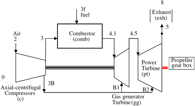
Data has been collected from engine test at acceleration over idle condition(Reference Baklacioglu, Aydin and Turan17,Reference Baklacioglu, Turan and Aydin18) . The aircraft is a small transport aircraft with two turbo-prop engines. It can carry up to six tons, and its maximum range is 5000km. Aircraft normal cruise speed is nearly 0.36 Mach. General schematic view of the engine and components are shown in Fig. 1. Engines can provide up to 1950 shaft horse power. It has gas generator, free turbine, and propeller gear box. Gas generator, or in other words the core engine, has an axial-radial compressor, a through-flow annular combustor, and a two-stage cooled turbine. Free turbine is un-cooled and consists of two stages. Propellers are variable pitch type, and they have reverse thrust capability. Engine is controlled through a digital engine controller and a hydro-mechanical fuel control unit. The generated power is extracted by free turbine and transmitted to the propeller gear box. Shaft torque and speed is measured during the engine run. This allows calculation of power transmitted to the propeller.
The schematic diagram of the turboprop engine (Ref. (Reference Wold5)).

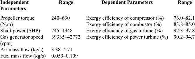
Propeller torque, shaft power, engine speed, air mass flow, and fuel flow rates have been measured and used as input data. Exergy efficiencies of the engine components have been calculated and Artificial Neural Network (ANN) learning methodology has been applied using the input information. Parameters and their ranges are given in Table 1. Normalised values given in references(Reference Baklacioglu, Turan and Aydin3) have been used for optimisation. The precision of each engine parameter is 6 decimal precision.
Turboprop engine parameters

In fact, fuel mass flow is the only real independent parameter that is manipulated by engine controller, and other parameters are dependent on it. However, component efficiencies and component matching reveals an implicit relation that may not show a direct linear relationship.
Since the engine characteristics are not provided by the manufacturer, it is required to find a formulation which will allow regeneration of the efficiency values using the input parameters. Spline modeling is a solution to this problem. Hundreds of data points can be represented with desired accuracy by using a small number of fitting points. As the number of fitting points increase, the accuracy of the spline function will also increase. It is aimed to use minimum number of points that provides required accuracy. Spline modeling was applied using two different point distribution and two different types of optimisation methods. Mean of the squared errors (MSE) is considered as objective function, and minimisation of the error by positioning the points is the optimisation problem. No constraints functions are used.
3.0 METHODOLOGY
Natural Cubic Spline algorithm(Reference Uyar and Ulker19) has been applied due to its simplicity. Spline is a composite curve that consists of many third-degree (fourth order) polynomials. The curves are connected at knot points such that the first and second derivatives are continuous; therefore, transitions at the joints are smooth(Reference Buchanan21). Spline fitting can be done using the given data points (fixed knots) or using arbitrary positions out of the data points (free knots) that gives the least squared error(Reference Kokkonis and Leute13). The method in this study is between fixed and free knot, namely semi-free knot method. Neither the given data points are directly used nor completely free-knot positions are used. Locations between the data points are searched by piecewise linear interpolation in order to find the smallest error. Since the data is not scattered, this approach is evaluated as more appropriate. Although the spline interpolation is a well-known subject, application of spline fitting to exergy efficiency data has not been used to date, a far as the authors are aware. This method is evaluated as a preferable method for modeling the non-linear exergy functions due to its accurate modeling ability.
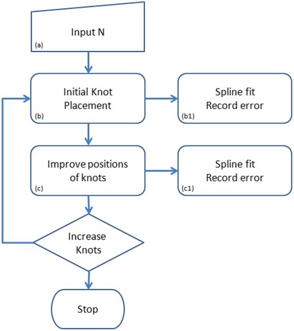
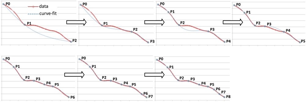
Exergy efficiency of the engine components shows different characteristics, and it is not possible to represent all the curves with same number of points. Therefore, in order to find the minimum number of knots that do not exceed acceptable error accuracy, these steps should be followed: (a) starting number of points is input to the program, (b) initial positioning is performed with method D1 or D2, spline is fitted and the mean of squared errors is recorded, and (c) optimisation algorithm (O1 or O2) is applied without changing the number of segments but only changing knot positions (Fig. 2) and the error is recorded. Calculations are automated by using a loop that increase fitting points starting from five. At each loop steps (b) and (c) are repeated until the loop counter exceeds the N.
Optimisation steps.

Two different knot placements are used in step (b):
• Distribution-1 (D1) : Equally spaced knots (de Boor and Rice)
• Distribution-2 (D2) : Inserting new knot at the maximum deviated location (Dierckx)
And two optimisation algorithms are applied in step (c):
• Optimisation –1 (O1) : Goldsection optimisation
• Optimisation –2 (O2) : Ant colony optimisation
Details of the knot placements and optimisation methods are given in the following paragraphs. In order to see effectiveness of the optimisation methodology, well-known titanium data(Reference de Boor and Rice10,Reference de Boor and Rice11) is used. Later, the same methodology is applied on the exergy efficiency data. Mean of Squared Errors (MSE) is used as criteria for selecting knot numbers. It has been predicted that 5-16 knots would give adequate accuracy. However, more knots are needed for some curves. Therefore, further spline fittings with higher knot numbers are applied in order to achieve desired accuracy.
Uniform spaced points (N = 8, 7 internal knots).

3.1 Initial knot placement - Step (b)
3.1.1 Uniform spaced points – D1
Figure 3 illustrates spline fitting with eight uniformly spaced points. Uniform spacing means equal length segments are applied along the X axis. It is based on minimum and maximum data points divided by equal number of segments. Y values corresponding to the curve at the X coordinates are selected as fitting points. After inserting the points, spline is fitted without optimisation,
 $$\matrix{
{{{\bf{X}}_{\rm{i}}} \in {{\rm{R}}^2},{\rm{S}} = \left\{ {{{\bf{X}}_{\rm{i}}}:{\rm{i}} = 0\;{\rm{to}}\;{\rm{m}}} \right\}} \cr
{{{\rm{X}}_{\rm{i}}}{\rm{ = }}\left\{ {{{\rm{x}}_{\rm{i}}},{\mkern 1mu} {{\rm{y}}_{\rm{i}}}} \right\}} \cr
} $$
Where m is the number of data points. Spline knot vector K is defined as
 $$\matrix{
{{{\rm{P}}_{\rm{j}}}{\rm{ = }}\left\{ {{{\rm{x}}_{\rm{j}}},{\mkern 1mu} {{\rm{y}}_{\rm{j}}}} \right\},{\rm{K = }}\left\{ {{{\rm{P}}_{\rm{j}}}:{\rm{j = 0}}\;{\rm{to}}\;{\rm{N}}} \right\}} \cr
{{{\rm{P}}_{\rm{0}}} < {{\rm{P}}_{\rm{1}}} < {{\rm{P}}_{\rm{2}}} < \ldots < {{\rm{P}}_{{\rm{N - 1}}}} < {{\rm{P}}_{{\rm{N}},}}} \cr
} $$
3.1.2 Adding knots at maximum deviated locations – D2
This method was introduced by Dierckx; however, the authors could not access the related publication. The original method is based on inserting knots until the required accuracy is reached. This way, only input accuracy specified and the algorithm finds knot positions and the number of knots. In this study, the number of points is specified at beginning. Initially there are two points — P0 and P1. Interim spline fitting is applied after in order to find the next deviated position. New point is added at the maximum deviated position. And the points are renumbered such that the minimum and maximum numbers will be at the ends of the curve. After inserting the specified number of knots residual, the spline is fitted without optimisation, and mean of squared errors is recorded. Knots adding sequence is illustrated in Fig. 4.
D2 method, knot adding sequence.

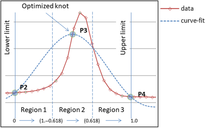
Boundaries for optimised knot.

3.2 Optimisation of internal knot positions – step (c)
3.2.1 Goldsection optimisation method – O1
This method(Reference Deb22) makes a line search in the specified region. Domain is divided in to three zones by using the golden number ratio (R = 0.618). Objective function is calculated (MSE) at the zone boundaries. And depending on theMSE, two of the regions are discarded. Next search is performed in the remaining zone until the minimum is found or maximum iteration number is reached. Only objective function evaluation is necessary, and it does not require derivation.
D1 or D2 placement gives an initial knot vector. The knot vector K = {Pj: j = 0, N} is used for calculation of the spline curve. At positions j = 0 and j = N the end points are located and their positions are fixed. Internal knot positions j = 1 through j = N − 1 are optimised. For a specific internal point (Fig. 5), position of the point is changed such that the least square error of the fitting will be achieved. Beginning from the P1 through PN−1, all internal knots are visited and better positions are searched using goldsection algorithm. This loop is repeated until no improvement is observed.
Lower and upper bounds for knot Pj are given as Pj−1 and Pj+1. MSE is used as objective function.
 $$Minimize\;||mse||\; = {1 \over m} \cdot \,\,{\mkern 1mu} \sum\limits_{i = 0}^m {{{\left( {f({x_i}) - s({x_i})} \right)}^2}} $$
subject to y j= s(x j) is spline function on knot vector P j = {x j, y j: j = 1,N} and x j ∈ (x j-1, x j+1)
3.2.2 Ant colony optimisation method – O2
The ant colony optimisation method is introduced by Dorigo in 1992(Reference Dorigo23). Later, many other ant colony algorithms with different foraging and searching approaches have been proposed. In this study the max-min ant system evaluation is used, which has been initially introduced by Thomas and Hoos(Reference Stützle and Hoos24). A good example of the ant colony optimisation is given in the book of Singiresu(Reference Rao25).
This method uses a number of ants with randomly searching a given region. The region is divided into discrete paths with equal pheromone level that makes equal probability of selection at the beginning. Every tour, all the ants are sent for searching randomly. When ants find food (better objective function values), pheromone levels of those paths are increased(Reference Deb22). Thus the chance of selection of these paths is increased. In order to simulate evaporation, pheromone levels are decayed after each tour. A decaying event increases the contrast between good and bad paths. In this study, the number of ants, number of paths, and decay coefficient are selected as 11, 14, and 0.3, respectively.
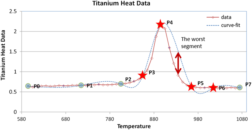
Ant colony optimisation knot selection.

In order to improve process effectiveness, a group of knots adjacent to the worst deviated segment is picked for optimisation. Positions of the knots are modified until the best MSE is found for the segment. As an example, selected knots are shown with stars on Fig. 6,
 $$Minimize\;||mse||\; = {1 \over m} \cdot {\mkern 1mu} \,\,\,\sum\limits_{i = 0}^m {{{\left( {f({x_i}) - s({x_i})} \right)}^2}} $$
subject to y j= s(x j), P j = {x j, y j: j = k − 2, k + 1} and x j ∈ (x j−1, x j+1)
where k is the worst segment number. At the beginning of each iteration, the worst segment is found and adjacent knots are picked for optimisation. If the first or last segment is the worst segment, only two knots are selected since end knots are not optimised. Iterations are applied until the improvement is negligible.
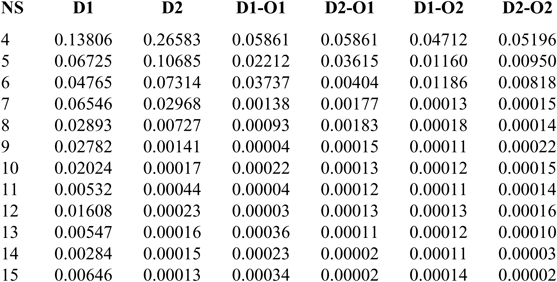
MSE summary for titanium data optimisation

R summary for titanium data optimisation

3.2 Titanium heat data
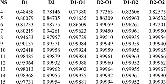
In order to check the successfulness of the spline fitting optimisation methodology in this study, cubic spline fitting study of Carl de Boor and John R. Rice(Reference Dierckx8,Reference Lu and Milios9) was used. De Boors used titanium heat data for first time in 1968 and since then it has been used as reference by many researchers. Application of the above-mentioned methodology is performed on the titanium heat data and results are evaluated. N is input as the number of spline segments, and knots are numbered from P0 to PN. Total number of knots is N + 1 and number of internal knots is N − 1. On titanium data, spline fitting is applied by changing N from 4 to 15. Summary of mean square error and R (linear correlation coefficient) are shown in Tables 2 and 3. In the headings
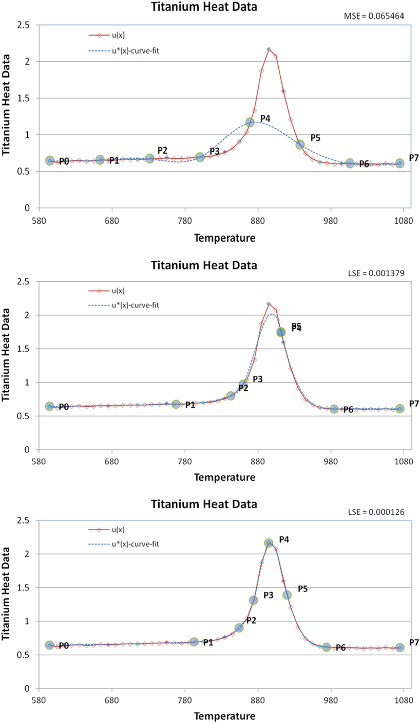
NS = 7 D1 (top), D1-O1 (mid) and D1-O2 (bottom).

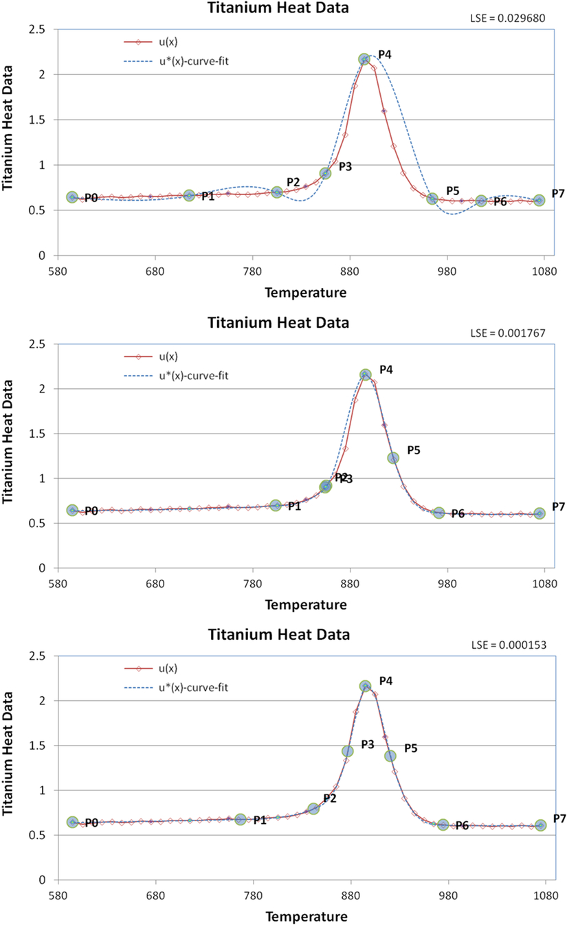
NS = 7 D2 (top), D2-O1 (mid) and D2-O2 (bottom).

• D1 - uniform distribution
• D2 - knots inserted according to Dierckx method
• O1 - goldsection optimisation is applied
• O2 - ant colony optimisation is applied
According to Tables 2 and 3, generally MSE and R values showed similar trend. As the NS is increased, MSE is decreased and R is increased. Accuracy improvement is faster for D2 comparing to the D1. Initial knot distribution also played a role in the optimisation results. The same optimisation method with different initial positions revealed different results. Thatindicates that initial positions of the knots can affect the LSE. For NS = 7, MSE obtained with D1-O2 and D2-O2 is better comparing to the other methods. Best result is obtained with D2-O1 NS = 14. For NS = 9, 11 and 12, D1-O1 also gave good results. Since the error difference is negligible, NS = 9 can be preferred instead of NS = 14.
For NS = 7, LSE = 0.00013 is still quite a good accuracy with only six internal knots. Initial and final positions of the knots are shown in Figs. 7 and 8.
As a result of this comparison it can be said that both the goldsection method and the ant colony optimisation methods provided good accuracy for this specific problem.
4. RESULTS AND DISCUSSION
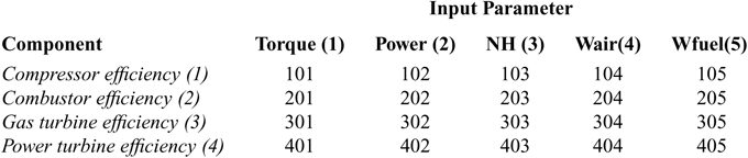
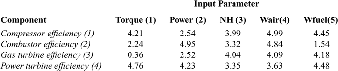
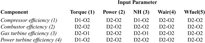
It is required to obtain mathematical models of the engine component exergy efficiencies by spline fitting. There is efficiency data for four engine components (compressor, combustor, gas turbine, and power turbine) and five engine inputs (propeller torque, shaft power, engine speed, air mass flow rate, and fuel flow rate). Thus, a matrix given in Table 4 is formed and 5 × 4 = 20 input-output pairs obtained. A unique number is assigned to pairs for convenience. Normalised range of the input and output parameters are given in Table 5.
Inputs and outputs matrix

Range of input and output parameters (normalised)

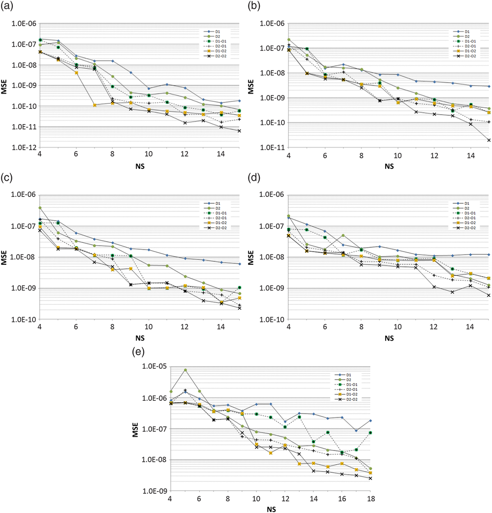
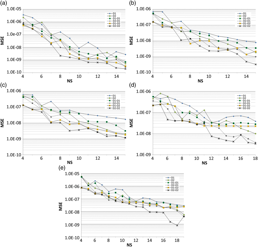
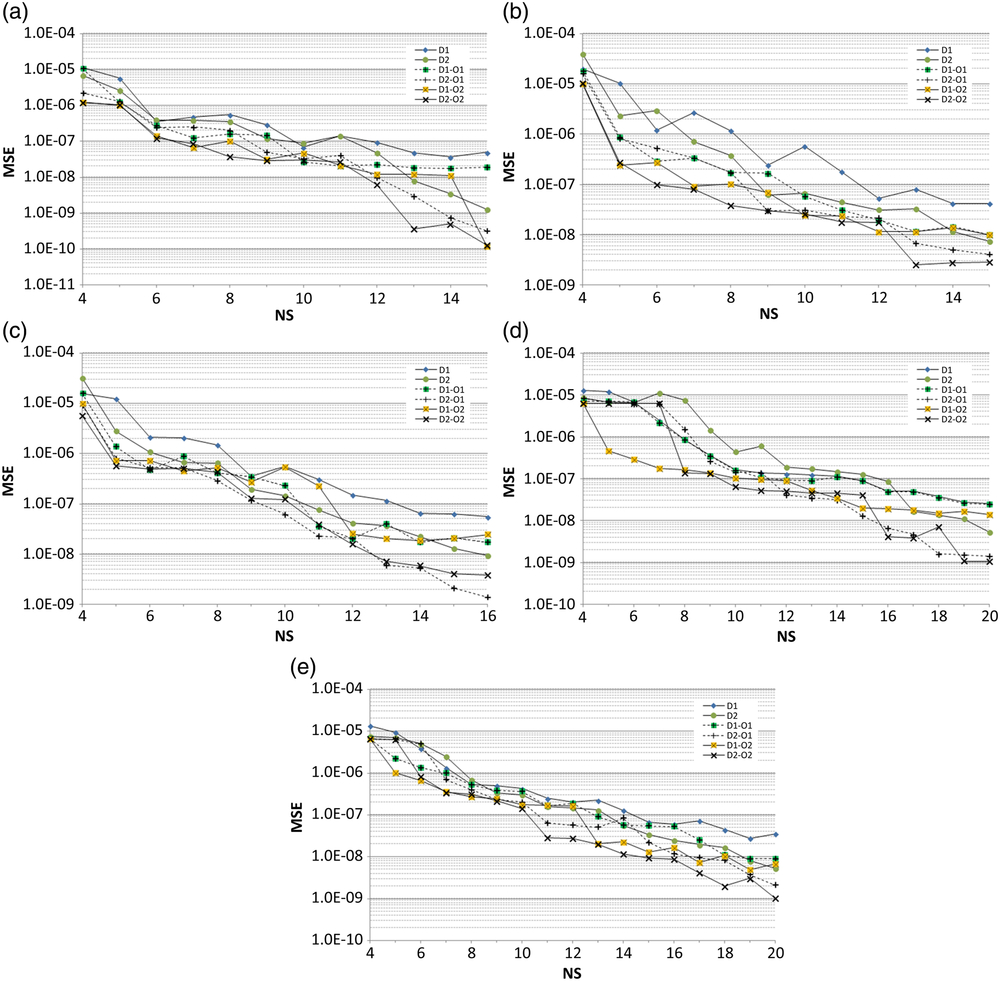
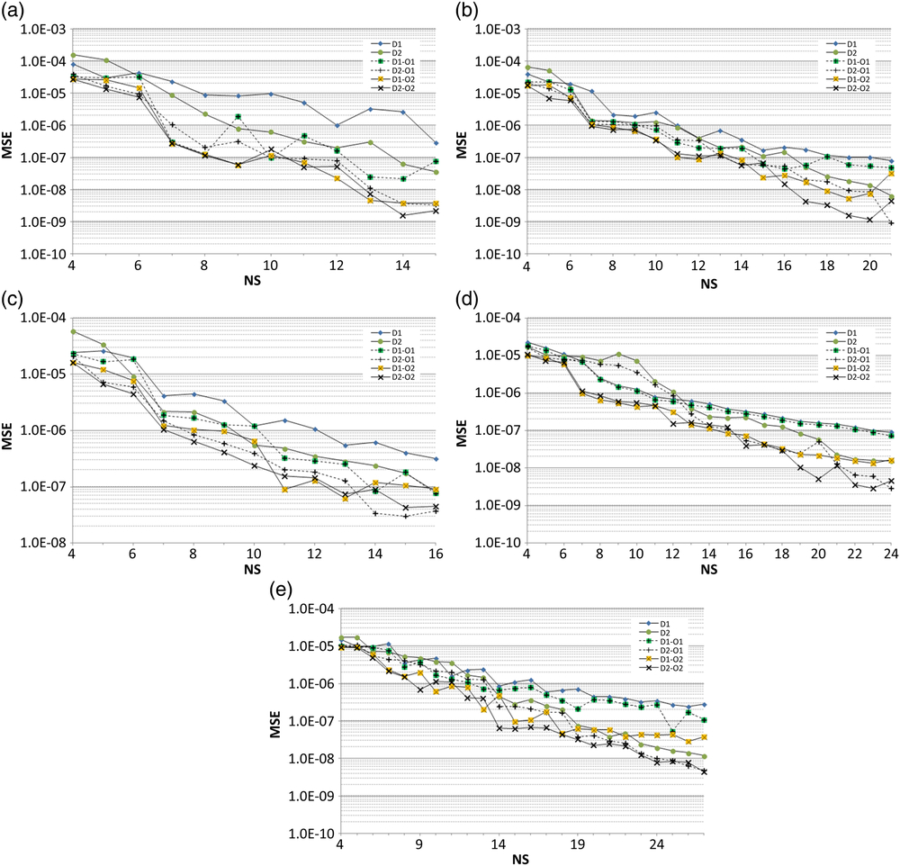
The practice in section 2.2 is applied to each pair. Graphical representations of MSE versus NS are given in Figs. 9–12. Related with the evaluated data, MSE values range between 10−4 and 10−11. Therefore logarithmic scale is used for MSE axis.
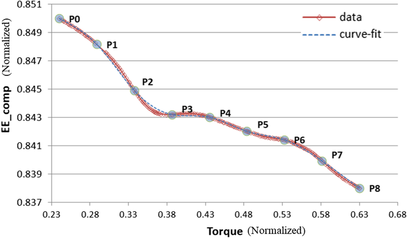
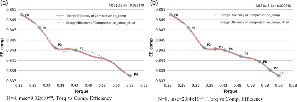
It is seen in all the figures that MSE values are very low, which can be misleading. For example case 101, NS = 4, MSE = 9.32 × 10⁻⁸ seems adequate accuracy. Maximum relative error in this case is 0.09%. By eye-check in Fig. 13(a), it can be seen that fitting curve does not overlap with the data very well whereas for N = 8, MSE = 2.84 × 10⁻⁹ and maximum relative error in this case is 0.02% and fitted curve and data showed negligible difference. Additionally, linear correlation coefficient “R” calculated for these cases are R = 0.99528 and R = 0.99985 respectively.
 $$Relative\;Error = Abs\left( {{{{y_i} - s\left( {{x_i}} \right)} \over {{y_i}}}} \right)$$
MSE-NS plots for (a) case 101, (b) case 102, (c) case 103, (d) case 104 and (e) case 105.

MSE-NS plots for (a) case 201, (b) case 202, (c) case 203, (d) case 204 and (e) case 205.

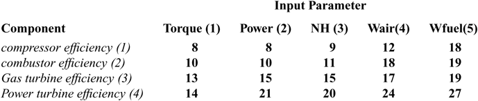
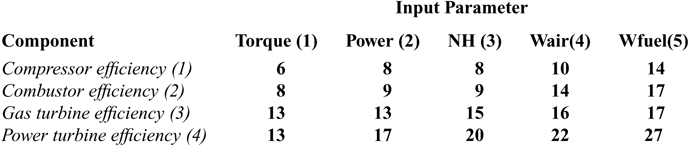
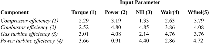
Considering the components and inputs matrix given in Table 2, there are 20 parameter pairs in total. For each pair two different distributions and two different optimisation algorithms have been applied. Spline fittings giving a MSE < 5.0 × 10⁻⁹ are selected as acceptable. It is observed that for MSE < 5.0 × 10⁻⁹, R value is always remained above 0.9998. In order to compare performance of optimisation methods O1 and O2, minimum knot numbers that provide the selected accuracy are put in to Tables 6 and 7. MSE values of these optimums are provided in Tables 8 and 9.
MSE-NS plots for (a) case 301, (b) case 302, (c) case 303, (d) case 304 and (e) case 305.

MSE-NS plots for (a) case 401, (b) case 402, (c) case 403, (d) case 404 and (e) case 405.

Acceptable accuracy comparison for optimisation: (a) N = 4, mse = 9.32 × 10−08, torq vs comp. efficiency and (b) n = 8, mse = 2.84 × 10−09, torq vs comp. efficiency.

For the cases 102, 301, 303, 403, and 405, both methods were able to provide acceptable accuracy with the same number of knots. At the other cases, O2 required less knots than O1. In order to see the combined effect of the distribution and optimisation, combinations providing the best spline fittings for each parameter pair are shown at Table 10. In 17 of 20 cases, D2-O2 combination has provided the best results.
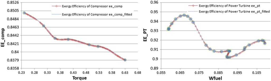
Compressor exergy efficiency versus torque (case 101) spline fitting required six knots and power turbine exergy efficiency versus fuel mass flow rate (case 405) spline fitting required 27 knots (Fig. 14). It can be seen that more complex curve requires more fitting points for getting an acceptable accuracy. Among the input parameters, Wair and Wfuel showed relatively complex behavior.
5.0 CONCLUSION REMARKS
Mathematical modeling with spline fitting helps reproducing engine exergy efficiency using smaller amount of data. Therefore it is convenient to represent the engine exergy efficiency curves using cubic splines. Another advantage of spline functions is that it is easy to get first and second derivations. Using goldsection and ant colony optimisation methods improved the spline fitting accuracy. For the same number of knots more accurate fitting can be obtained. Or desired accuracy can be reached using less number of knots. It should be noted that, although the calculation efforts are not compared as a criterion while evaluating the results, none of the methods gave significantly better calculation effort.
Minimum number of knots for MSE ≤ 5 × 10⁻⁹ accuracy (using O1 optimisation method)

Minimum number of knots for MSE ≤ 5 × 10⁻⁹ accuracy (using O2 optimisation method)

MSE obtained using O1 optimisation method (×10−09)

MSE obtained using O2 optimisation method (×10−09)

Effect of distribution type

Simple and complex data modeling examples (case 101 and case 405).

As a first attempt and novelty in the current literature, in this study it is shown that in context of engine exergy efficiency, input-output parameter mathematical modeling, spline fitting with ant colony optimisation provided good results comparing to the gold section.
ACKNOWLEDGEMENT
The authors would like to thank Eskisehir Technical University and Tusas Engine Industries (TEI) in Turkey for their support.