



1. Introduction
The coating of a solid surface by a thin liquid film is ubiquitous in nature. It is important in a wide range of biological (such as the thin mucus layer coating the walls of mammalian lung airways and tear films coating the eyeball) and industrial (such as in paint coating and computer microchip production) applications. In these applications, understanding the physics of the spreading process is of great importance in order to minimise undesirable effects leading to dry areas and imperfections. The spreading or coating process develops as a balance between viscous and surface tension forces; in some configurations, body forces, such as gravity, are also relevant to drive the spreading flow. In many technological applications, surfactants are used to control the spreading of liquids, owing to their ability to modify the surface tension at the liquid–air interface (Rosen Reference Rosen2004). Common applications that exploit the properties of surfactants include detergents, crop spraying, coating processes, microfluidics and oil recovery. Surfactants also occur naturally in the mammalian lung. They reduce the surface tension of the mucus layer lining the lung airways, which assists in preventing the collapse of the smaller airways (Grotberg Reference Grotberg1994, Reference Grotberg2001). In the lungs of premature infants, the quantity of surfactant produced is insufficient, as the lungs are underdeveloped. This leads to a respiratory distress syndrome, which is treated by surfactant replacement therapy (SRT). SRT involves delivering artificial surfactant into the lung exogenously. It then spreads under the action of surface tension gradients and to a lesser extent gravity so as to coat the airways, ideally as uniformly as possible.
Thin liquid films spreading on solid substrates driven by external forces such as gravity, or due to surfactant-related effects, exhibit intriguing instabilities resulting in the formation of a range of striking patterns. The gravity-driven spreading of a drop or sheet down an inclined substrate develops a finger-like instability due to transverse perturbations in the flow. This experiment was first conducted by Huppert (Reference Huppert1982) and then expanded on by Silvi & Dussan (Reference Silvi and Dussan1985), Jerrett & de Bruyn (Reference Jerrett and de Bruyn1992) and Hocking, Debler & Cook (Reference Hocking, Debler and Cook1999), among others. Triangular sawtooth-like patterns have been observed experimentally at small inclination angles or for a completely wetting fluid. For larger inclination angles or for a partially wetting fluid, the instability looks more finger-like, with the sides of the fingers rounded and almost parallel. A completely different fingering instability is observed in the case when surfactant is present. This fingering behaviour was first observed by Marmur & Lelah (Reference Marmur and Lelah1981) and then expanded on by Afsar-Siddiqui and co-workers (Afsar-Siddiqui, Luckham & Matar Reference Afsar-Siddiqui, Luckham and Matar2003a ,Reference Afsar-Siddiqui, Luckham and Matar b ,Reference Afsar-Siddiqui, Luckham and Matar c , Reference Afsar-Siddiqui, Luckham and Matar2004). In contrast to the fingering instability observed during gravity-driven spreading, the fingers here are more dramatic (often referred to as dendritic) and are of a much smaller length scale. The interested reader is referred to the recent articles by Craster & Matar (Reference Craster and Matar2009) and Matar & Craster (Reference Matar and Craster2009) for a thorough review of experimental and theoretical research in surfactant-related fingering instabilities in thin-film spreading flows. As the angle of inclination is increased from the horizontal, the effects of gravity will begin to compete with that due to surfactant. To the best of our knowledge, there are no experiments for surfactant and gravity-driven spreading on inclined planes to describe these competing effects. To gain a better theoretical understanding of this, we consider here a model problem involving the spreading and stability of a surfactant-laden drop on an inclined plane coated with an initially uniform (and surfactant-free) liquid film.
To set this problem in context, it is useful first to recall some key features of drop spreading on a solid substrate. One is the existence of a free surface at the liquid–vapour interface, which evolves in time as a consequence of the balance between the driving forces. The other is the presence of a moving contact line at the boundary between the liquid, the vapour and the solid substrate. The combination of these two characterises the stability of the spreading flow, with non-trivial shapes of the free surface and corrugations of the contact line. At the moving contact line, imposing a no-slip condition leads to a non-integrable stress singularity, the so-called ‘contact-line paradox’ (Huh & Scriven Reference Huh and Scriven1971; Dussan & Davis Reference Dussan and Davis1974). Numerous regularisations have been proposed to remedy this, such as allowing the liquid to slip on the solid substrate (referred to as a slip condition) or assuming that the solid substrate is prewetted with a precursor liquid film. Incorporating a precursor film, such that the spreading front of the drop only has effective or apparent contact with the precursor film, allows the no-slip boundary condition still to be imposed without being contradictory. In this work, we use a precursor film, owing to the simplicity in its implementation in comparison to the other regularisations.
The gravity-driven spreading of a viscous drop or sheet on a prewetted inclined plane has been the focus of numerous theoretical studies. This problem was first studied for flow down a vertical plane by Huppert (Reference Huppert1982), who identified a similarity solution for the spatially one-dimensional fluid sheet thickness,
 $h\sim \sqrt{x}$
(where
 $x$
is the distance in the flow direction and
 ${\sim}$
denotes ‘scales like’). This work was extended, particularly, by Troian et al. (Reference Troian, Herbolzheimer, Safran and Joanny1989) and Hocking (Reference Hocking1990), who revealed a late-time multi-region asymptotic solution structure, with the bulk drop or sheet, characterised by Huppert’s similarity solution, connecting two short transition regions at the leading and trailing edges where surface tension (or capillary) effects are important and are comparable to gravitational forces. Using matched asymptotic analysis, they showed that the one-dimensional flow in the transition region at the leading edge of the drop is characterised by a family of quasi-steady solutions parametrised by the ratio of the precursor film thickness and the drop height far upstream of this region. These solutions accommodate a bulge in the drop height referred to as a capillary ridge. A linear stability analysis of this region to transverse perturbations was performed by extracting the growth rate of the perturbations to a ‘frozen’-in-time base state represented by a particular solution curve in the family of quasi-steady solutions. The dispersion relation between the growth rate and transverse wavenumber showed that this region is linearly unstable to long-wavelength perturbations with a well-defined maximum growth rate and wavenumber, with short wavelengths stabilised by surface tension. A small-wavenumber analysis showed the leading-order behaviour to be
 $O(q^{2})$
(where
 $q$
is the wavenumber) and a stability criterion was obtained revealing that the capillary ridge is necessary for the instability to develop. This suggested that the transition region at the leading edge of the spreading drop could be a precursor to the fingering instability observed in experiments. Hocking (Reference Hocking1990) also showed that the bulk drop spreads in time
 $t$
like
 $t^{1/3}$
and thins like
 $t^{-1/3}$
. Bertozzi & Brenner (Reference Bertozzi and Brenner1997) extended the analysis to the general case of flow down an inclined plane from a constant-flux fluid source. They showed the existence of a travelling wave solution for the one-dimensional flow. A linear stability analysis of this solution to transverse perturbations showed that flow becomes less linearly unstable as the inclination angle decreases, and below a critical angle the flow is linearly stable. This is necessarily due to a decrease in the thickness of the capillary ridge, which is less pronounced at low inclination angles. The constant-flux configuration has been used in several subsequent studies to analyse a variety of effects, such as viscoelasticity (Spaid & Homsy (Reference Spaid and Homsy1996) – who also compared the effects of a precursor film and slip condition at the moving contact line and found the results to be similar). Two-dimensional numerical studies (Schwartz Reference Schwartz1989; Eres, Schwartz & Roy Reference Eres, Schwartz and Roy2000; Kondic & Diez Reference Kondic and Diez2001, Reference Kondic and Diez2002) have been able to reproduce the fingering patterns, providing quantitative agreement with experiments.
In comparison, the theoretical study of surfactant-driven spreading is relatively young (Craster & Matar (Reference Craster and Matar2009) and Matar & Craster (Reference Matar and Craster2009) provide good reviews of the latest analytical and numerical research in this area). The main focus has been on drop spreading on a horizontal prewetted and surfactant-free substrate. Troian, Herbolzheimer & Safran (Reference Troian, Herbolzheimer and Safran1990) first investigated theoretically the one-dimensional axisymmetric flow structure, which included, ahead of the leading edge of the spreading bulk drop, a propagating fluid front (also referred to as a spreading monolayer) with a kinematic shock at its leading edge. The large initial surfactant concentration gradient that exists between the edge of the drop and the surfactant-free precursor film results in a large surface-tension gradient, causing fluid to be ‘sucked’ from the precursor film by the Marangoni effect forming the fluid front, which propagates ahead of the bulk drop. This results in strong stretching of the film’s interface, causing severe thinning of the precursor film just ahead of the drop’s effective contact line. The drop therefore has to spread over an extremely thin surfactant-loaded liquid film. In doing so, the advancing contact line can develop the fingering patterns observed in experiments. Troian et al. (Reference Troian, Herbolzheimer and Safran1990) proposed qualitatively a physical mechanism giving rise to the observed fingering. Identifying an ‘adverse mobility gradient’ between the thicker bulk drop and thinner precursor film, they suggested an analogy with the viscous fingering in a Hele-Shaw cell where a more mobile (less viscous) fluid displaces a less mobile (more viscous) one (Homsy Reference Homsy1987). The fluid front and kinematic shock have been independently analysed in a related problem of an insoluble surfactant monolayer spreading on an initially planar film. Jensen & Grotberg (Reference Jensen and Grotberg1992) described the spatially one-dimensional structure using a variety of similarity solutions (see also Jensen Reference Jensen1994). Of particular relevance to this work is their similarity solution for a planar geometry, which at leading order showed that the thickness of the front varies linearly in the streamwise direction, the thickness at its leading edge is equal to twice the precursor thickness and it spreads in time
 $t$
like
 $t^{1/3}$
. Warner, Craster & Matar (Reference Warner, Craster and Matar2004) extended the study by Troian et al. (Reference Troian, Herbolzheimer and Safran1990), describing the flow using two coupled nonlinear partial differential equations (PDEs) for the evolution of the drop height or film thickness and the surfactant concentration. Their spatially one-dimensional simulations revealed a structure broadly similar to that described by Troian et al. (Reference Troian, Herbolzheimer and Safran1990), with the bulk drop connecting to the fluid front via an ultra-thin film. They also examined the stability of their spatially one-dimensional numerical solution to small-amplitude transverse perturbations using a transient growth analysis, where the growth of perturbations is measured by a suitable norm. Their stability analysis showed sustained growth of disturbances concentrated around the edge of the bulk drop’s effective contact line. Their two-dimensional computations revealed fingering patterns resembling those seen in experiments. Jensen & Naire (Reference Jensen and Naire2006) revisited the problem and, by exploiting high-resolution numerical simulations, they were able to describe, using matched asymptotic analysis, the late-time multi-region asymptotic spatially one-dimensional flow structure, using which the spreading and thinning rates were determined. In particular, they were able to show that the local solution structure near the drop’s effective contact line can be described using the Landau–Levich equation. They examined the linear stability of this region to transverse perturbations and showed it to be linearly unstable to long-wavelength perturbations with a well-defined maximum growth rate and wavelength. Using long-wavelength asymptotics, they showed the leading-order behaviour of the dispersion relation between the growth rate and the transverse wavenumber to be
 $O(q)$
and derived a stability criterion that revealed the destabilising influence of surfactant via the Marangoni effect.
Only a few studies have examined theoretically the spreading of a surfactant-laden drop on a prewetted and inclined substrate. This problem was first studied by Edmonstone, Matar & Craster (Reference Edmonstone, Matar and Craster2004, Reference Edmonstone, Matar and Craster2005a ,Reference Edmonstone, Matar and Craster b , Reference Edmonstone, Matar and Craster2006) for both constant-volume and constant-flux configurations. Their spatially one-dimensional constant-volume numerical simulations revealed a solution structure that showed the spreading bulk fluid drop with a capillary ridge at its leading edge, reminiscent of gravity-driven spreading. Ahead of and behind the leading and trailing edges of the spreading drop, respectively, there are propagating fluid fronts driven by the Marangoni effect, with the front ahead of the drop’s leading edge looking more like a ‘step’ for small precursor film thicknesses. They also observed a slight upwelling of fluid (so-called ‘fluid hump’) between the main bulk drop and the capillary ridge due to the Marangoni effect. Figure 2 shows a numerical simulation illustrating the above features. Their spatially one-dimensional flow results also showed surfactants to slow down the spreading of the bulk drop compared to spreading due to gravity alone. They used transient growth analysis and fully nonlinear simulations to explore the stability of their spatially one-dimensional solution to transverse perturbations in the flow and surfactant concentrations. They found that the flow is linearly unstable to long-wavelength perturbations, with sustained growth of disturbances concentrated near the drop’s leading-edge effective contact line. They speculated that the base flow was always linearly unstable for all inclination angles, in contrast to gravity-driven spreading, which is linearly stable below a critical angle (Bertozzi & Brenner Reference Bertozzi and Brenner1997). Their two-dimensional numerical simulations confirmed the results from the transient growth analysis, clearly showing perturbations to develop into long distinct fingers. Edmonstone et al. (Reference Edmonstone, Matar and Craster2006) extended the study to include surfactant solubility effects. They showed that solubility effects add to the destabilising influence of surfactants. These works were further extended by Mavromoustaki (Reference Mavromoustaki2011) and Mavromoustaki, Matar & Craster (Reference Mavromoustaki, Matar and Craster2012a ,Reference Mavromoustaki, Matar and Craster b ) to investigate the climbing of a surfactant-laden film against the influence of gravity. They also explored the linear and nonlinear stability of the spatially one-dimensional flow using transient growth analysis and two-dimensional simulations. They found that the surfactant concentration gradient behind the leading-edge effective contact line was important in the development of the fingering instability.
Levy & Shearer (Reference Levy and Shearer2006) theoretically investigated the slightly simpler scenario of a spatially one-dimensional flow of a surfactant-laden fluid layer down an inclined and prewetted substrate from a constant-flux source, neglecting surface tension and surface diffusion effects. They showed that the one-dimensional flow structure admits a combination of travelling waves, some in which the fluid height is piecewise constant and the surfactant concentration is piecewise linear and continuous. The entire long-time structure is shown to be a single travelling wave in which disturbances propagate towards the leading edge. Below a critical ratio of upstream to downstream height, they derived an exact solution representing a triple-step travelling wave in which the height is piecewise constant and the surfactant concentration is piecewise linear and has compact support. A subsequent study by Levy, Shearer & Witelski (Reference Levy, Shearer and Witelski2007) expanded on this work, including surface tension effects to describe the leading-edge effective contact-line region of the spreading film. They showed that the length of this region scales like
 $\mathit{Ca}^{1/3}$
, where
 $\mathit{Ca}$
is a capillary number. A travelling wave solution structure was postulated based on the numerical solutions, resulting in a third-order differential equation for the height of the fluid layer coupled to a first-order differential equation for the surfactant concentration. A partial analysis of these differential equations was done using a combination of asymptotics and phase-plane analysis. We remark that, although the solution structure for the surfactant-laden drop spreading problem presented in our work here has close analogies with that described by Levy and co-workers, it has no travelling wave structure. Moreover, the presence of long-lived transient dynamics also makes any analytical description of the long-time asymptotic structure much more complicated than the travelling wave analysis (as described in § 4).
In this paper, we revisit the spatially one-dimensional spreading of a drop treated by Edmonstone et al. (Reference Edmonstone, Matar and Craster2004, Reference Edmonstone, Matar and Craster2005a ,Reference Edmonstone, Matar and Craster b ) for a constant-volume configuration (see figure 1 for a schematic of this). We use high-resolution numerical simulations and asymptotic approximations to describe the late-time multi-region self-similar solution structure. These include the drop’s leading-edge effective contact-line region, which is described as a family of quasi-steady solutions for the drop height and surfactant concentration parametrised by the effective contact-line speed, the ratio of the downstream and upstream film thicknesses, and the ratio of the upstream and downstream surfactant concentration gradients. A differential–algebraic equation (DAE) model is derived for the evolution of key variables characterising the spreading process, using which spreading and thinning rates are determined. We then examine the stability of the leading-edge effective contact-line region. Assuming that this region evolves slowly enough that we may treat the base state as ‘frozen’ in time (represented by a particular solution curve in the family of quasi-steady solutions), a linear stability analysis reveals an exponential growth rate for disturbances as a function of the transverse wavenumber. We describe this relationship in the limit of small wavenumber asymptotically and finite-wavenumber effects numerically. This enables us to identify physical mechanisms and new scaling properties of the instability.
Schematic of a surfactant-laden drop spreading on an inclined and prewetted plane.

2. The model
We consider the spreading of a drop of surfactant-laden liquid down a plane inclined at angle
 ${\it\theta}$
to the horizontal that is prewetted with a thin layer of the same liquid, uncontaminated by surfactant (see figure 1). Initially, the drop has maximum height
 $H^{\star }$
and width
 $H^{\star }/{\it\epsilon}$
(for some
 ${\it\epsilon}\ll 1$
); the precursor layer has thickness
 ${\it\delta}H^{\star }$
(for some
 ${\it\delta}\ll 1$
) and uniform surface tension
 ${\it\sigma}^{\star }$
. The liquid has constant viscosity
 ${\it\mu}^{\star }$
, density
 ${\it\rho}^{\star }$
and the spreading motion is assumed slow enough that inertial effects may be neglected. Insoluble surfactant is present on the drop initially at concentration
 ${\it\Gamma}^{\star }$
, lowering the surface tension of the drop to
 ${\it\sigma}^{\star }-S^{\star }$
(
 $S^{\star }$
being the drop’s spreading coefficient). The surfactant concentration is assumed sufficiently dilute that
 $S^{\star }\ll {\it\sigma}^{\star }$
, so that the equation of state relating surface tension to surfactant concentration may be assumed linear (with slope
 $-S^{\star }/{\it\Gamma}^{\star }$
). The surfactant diffuses on the interface with diffusivity
 $D_{s}^{\star }$
.
Lubrication theory can be used to derive evolution equations governing the spreading of the surfactant-laden drop over the precursor film (see Edmonstone et al.
Reference Edmonstone, Matar and Craster2004, Reference Edmonstone, Matar and Craster2005a
,Reference Edmonstone, Matar and Craster
b
). We scale the drop height on
 $H^{\star }$
, distance along the plane on
 $H^{\star }/{\it\epsilon}$
, pressure on
 $({\it\rho}^{\star }g^{\star }\sin ({\it\theta})H^{\star })/{\it\epsilon}$
, time on
 ${\it\mu}^{\star }/({\it\epsilon}{\it\rho}^{\star }g^{\star }\sin ({\it\theta})H^{\star })$
and surfactant concentration on
 ${\it\Gamma}^{\star }$
. These are derived based on a characteristic velocity
 $U^{\star }=({\it\rho}^{\star }g^{\star }\sin ({\it\theta})H^{\star \,2})/{\it\mu}^{\star }$
obtained by balancing the horizontal component of gravity with viscous forces, where
 $g^{\star }$
is the acceleration due to gravity. The evolution equations for the film thickness,
 $h(x,y,t)$
, and surfactant concentration,
 ${\it\Gamma}(x,y,t)$
, are
 $$\begin{eqnarray}\displaystyle & h_{t}=\boldsymbol{{\rm\nabla}}\boldsymbol{\cdot }(-{\textstyle \frac{1}{3}}\mathit{Ca}\,h^{3}\boldsymbol{{\rm\nabla}}{\rm\nabla}^{2}h+{\textstyle \frac{1}{3}}Dh^{3}\boldsymbol{{\rm\nabla}}h+{\textstyle \frac{1}{2}}h^{2}M\boldsymbol{{\rm\nabla}}{\it\Gamma})-({\textstyle \frac{1}{3}}h^{3})_{x}, & \displaystyle\end{eqnarray}$$
 $$\begin{eqnarray}\displaystyle & \displaystyle {\it\Gamma}_{t}=\boldsymbol{{\rm\nabla}}\boldsymbol{\cdot }\left(-\frac{1}{2}\mathit{Ca}\,h^{2}{\it\Gamma}\boldsymbol{{\rm\nabla}}{\rm\nabla}^{2}h+\frac{1}{2}Dh^{2}{\it\Gamma}\boldsymbol{{\rm\nabla}}h+Mh{\it\Gamma}\boldsymbol{{\rm\nabla}}{\it\Gamma}\right)-\left(\frac{1}{2}h^{2}{\it\Gamma}\right)_{x}+\frac{{\rm\nabla}^{2}{\it\Gamma}}{\mathit{Pe}},\qquad & \displaystyle\end{eqnarray}$$
We work in the domain
 $-\infty <x<\infty$
,
 $0\leqslant y\leqslant 2{\rm\pi}/k$
for some fixed
 $k$
, and impose the boundary conditions
 $h\rightarrow {\it\delta}$
and
 ${\it\Gamma}\rightarrow 0$
as
 $x\rightarrow \pm \infty$
and periodicity in
 $y$
. Following Edmonstone et al. (Reference Edmonstone, Matar and Craster2004, Reference Edmonstone, Matar and Craster2005a
,Reference Edmonstone, Matar and Craster
b
), the initial conditions are as follows:
 $h(x,y,0)=(1+{\it\delta}-x^{2})[H(1-x)-H(-1-x)]+{\it\delta}[H(x-1)+H(-1-x)]$
and
 ${\it\Gamma}(x,y,0)=H(1-x)-H(-1-x)$
, where
 $H(x)=[1+\tanh (Kx)]/2$
. This represents a parabolic drop shape with leading edge at
 $x=1$
and trailing edge at
 $x=-1$
connecting onto a precursor film of thickness
 ${\it\delta}$
. The surfactant concentration is uniform over the drop, with steep concentration gradients at the leading and trailing edges.
The problem is parametrised by:
 ${\it\delta}$
, the dimensionless precursor thickness;
 $K$
, controlling the shape of the initial conditions;
 $\mathit{Ca}={\it\epsilon}^{3}{\it\sigma}^{\star }/({\it\mu}^{\star }U^{\star })$
, an inverse capillary number (compares surface tension to viscous forces);
 $M={\it\epsilon}S^{\star }/({\it\mu}^{\star }U^{\star })$
, a Marangoni number (compares surface tension gradient to viscous forces and is related to the strength of the surfactant system);
 $D={\it\epsilon}\cot ({\it\theta})$
, related to the inclination angle
 ${\it\theta}$
; and
 $\mathit{Pe}=U^{\star }H^{\star }/({\it\epsilon}D_{s}^{\star })$
, a Péclet number (compares the magnitude of surfactant transport due to advection and diffusion).
In § 3 we use a finite difference method to compute
 $y$
-independent solutions of (2.1) satisfying
 $$\begin{eqnarray}\displaystyle & h_{t}+Q_{x}=0,\quad Q\equiv {\textstyle \frac{1}{3}}\mathit{Ca}\,h^{3}h_{xxx}-{\textstyle \frac{1}{3}}Dh^{3}h_{x}-{\textstyle \frac{1}{2}}Mh^{2}{\it\Gamma}_{x}+{\textstyle \frac{1}{3}}h^{3}, & \displaystyle\end{eqnarray}$$
 $$\begin{eqnarray}\displaystyle & \displaystyle {\it\Gamma}_{t}+q_{x}=0,\quad q\equiv \frac{1}{2}\mathit{Ca}\,h^{2}{\it\Gamma}h_{xxx}-\frac{1}{2}Dh^{2}{\it\Gamma}h_{x}-Mh{\it\Gamma}{\it\Gamma}_{x}+\frac{1}{2}h^{2}{\it\Gamma}-\frac{1}{\mathit{Pe}}{\it\Gamma}_{x}, & \displaystyle\end{eqnarray}$$
 $Q$
and
 $q$
are fluid and surfactant fluxes, respectively. Our numerical scheme employed a fixed but spatially non-uniform grid, with grid points clustered in regions where we anticipated rapid spatial variation. We used implicit time stepping and validated convergence using grid refinement. For the simulations shown, the grid spacing varied from
 $10^{-4}$
where the film was extremely thin (particularly around the trailing edge of the drop) to
 $10^{-3}$
elsewhere. The overall features of the flow are as reported by Edmonstone et al. (Reference Edmonstone, Matar and Craster2004, Reference Edmonstone, Matar and Craster2005a
,Reference Edmonstone, Matar and Craster
b
). Our finer computational grid allows us to resolve some important details not described previously. Moreover, we compute solutions to much longer times than reported previously, which allows us to describe theoretically their asymptotic structure.
Late-time evolution of (a) film thickness
 $h$
and (b) surfactant concentration
 ${\it\Gamma}$
for
 $t=(0.001,0.01,0.1,0.2,0.5,1)\times 10^{6}$
(see text for parameter values). Late-time solution structure of (c) film thickness
 $h$
and (d) surfactant concentration
 ${\it\Gamma}$
at
 $t=5\times 10^{5}$
. Insets in (c) show the capillary ridge, fluid fronts near the leading and trailing edges of the drop, and the ultra-thin film near the drop’s trailing edge. The inset in (d) shows the steep drop in surfactant concentration immediately ahead of the maximum surfactant concentration.

3. Drop spreading: numerical results
Figure 2(a,b) shows numerical simulations of (2.2) at late times (
 $t=10^{3}{-}10^{6}$
) for
 $h$
and
 ${\it\Gamma}$
, respectively. The parameter values are:
 $\mathit{Ca}=10^{-3}$
,
 $M=1$
,
 ${\it\delta}=10^{-3}$
,
 ${\it\theta}=90^{\circ }$
,
 $\mathit{Pe}=10^{5}$
and
 $K=100$
. At these times, the solution exhibits the structure shown in figure 2(c,d) (which shows the evolution of
 $h$
and
 ${\it\Gamma}$
at
 $t=5\times 10^{5}$
). This illustrates the dramatic variation in film thickness between the bulk drop (where
 $h=O(1)$
), the precursor film thickness (where
 $h={\it\delta}=10^{-3}$
) and the ultra-thin film behind the trailing-edge contact line (see inset in figure 2
c, where
 $h$
decreases to around
 $10^{-4}$
). The spreading of the bulk drop is characteristic of gravity-driven spreading with a capillary ridge at its leading edge (see inset in figure 2
c). The height of the capillary ridge decreases as the inclination angle decreases. The influence of surfactant is evident in the upwelling of fluid just behind the capillary ridge (see figure 2
c; hereafter referred to as a fluid ‘hump’) and fluid fronts (where
 $h=O({\it\delta})$
) observed both upstream and downstream of the spreading drop (see insets in figure 2
c). This is caused by gradients in surface tension arising due to surfactant concentration gradients. At the downstream fluid front, the surfactant concentration is linear and decreasing (see figure 2
d), the resulting Marangoni flow causing this front to develop and spread down the inclined plane. At the upstream fluid front, the surfactant concentration is linear and increasing (see figure 2
d), the resulting reverse Marangoni flow causing this front to spread up the inclined plane (against the direction of the horizontal component of gravity). It is worth noting that, for the value of the precursor thickness
 ${\it\delta}=10^{-3}$
chosen in the numerical simulations shown here, the downstream fluid front appears to look like a ‘step’ (see inset in figure 2
c). As the precursor thickness is increased, the slope of this fluid front increases and it looks more like the fluid front at the upstream end (Edmonstone et al.
Reference Edmonstone, Matar and Craster2005b
). The fluid hump behind the capillary ridge is also due to a reverse Marangoni flow (the surfactant concentration is almost linear and increasing; see figure 2
d) impeding the downward flow due to gravity, resulting in the fluid swelling up. The surfactant concentration in the majority of the bulk drop is roughly constant (figure 2
d). For later reference, we also note the steep drop in the surfactant concentration immediately ahead of the maximum surfactant concentration (see inset in 2
d). The ultra-thin film (see figure 2
c) is a consequence of flow being sucked away from the precursor film into the upstream fluid front, causing it to thin severely.
Late- to late-late-time evolution of film thickness
 $h$
upstream of the trailing edge of the drop. The parameter values are:
 $\mathit{Ca}=10^{-3}$
,
 $M=1$
,
 ${\it\delta}=10^{-3}$
,
 ${\it\theta}=90^{\circ }$
,
 $\mathit{Pe}=10^{5}$
and
 $K=100$
. The inset shows the early development of a structure resembling the leading-edge capillary ridge.

The structure of the bulk drop and the downstream fluid front shown in figure 2(c,d) is robust for a range of parameter values (for inclination angle not close to the horizontal) and persist even at very late times. However, the structures behind the trailing edge are not. Figure 3 shows the evolution of the film thickness at late to late-late times (
 $t=10^{3}$
to
 $5\times 10^{6}$
), where the surfactant concentration gradient there has reduced significantly for it not to be able to counteract the downward flow due to horizontal gravity. The fluid in the front now flows back due to gravity, and we speculate that it will eventually result in a structure resembling the capillary ridge at the leading edge of the drop. An early indication of this can be observed in figure 3 at
 $t=(4,5)\times 10^{6}$
(see solid and dash-dotted lines in the inset shown). Indeed, late-time simulations for smaller Marangoni numbers (not shown here) clearly indicate the formation of a satellite capillary ridge region, which connects directly onto the trailing edge of the bulk drop.
A sketch of the late-time asymptotic structure shown in figure 2, showing film thickness
 $h$
and surfactant concentration
 ${\it\Gamma}$
as functions of distance
 $x$
from the trailing edge of the drop. Dashed lines demarcate asymptotic regions: the main bulk drop (I), the fluid hump (II), the fluid front (III), the precursor film (IV), the drop’s leading-edge effective contact line (A), and the shock-like structures (B) and (C).

As might be anticipated from figure 2(a,b), much of the late-time spreading is locally self-similar, with solution structure illustrated in figure 2(c,d). The upstream structures resemble closely (at least for the times considered here) those observed when a surfactant-laden drop spreads on a horizontal plane, whose self-similar structure is discussed in detail in Jensen & Naire (Reference Jensen and Naire2006); hence we do not include their description here. Moreover, numerical simulations show almost negligible fluid or surfactant flux across the trailing edge of the drop, which enables us to decouple the spreading dynamics of the bulk drop and downstream structures from the upstream ones. Our main focus here is in describing the spreading dynamics of the bulk drop and the structures downstream whose self-similar structure we examine in more detail in § 4.
4. Drop spreading: asymptotic approximation
We postulate a late-time asymptotic structure consisting of seven regions, four long (I, II, III and IV) and three short (A, B and C) (sketched in figure 4), from which we derive an approximate DAE model describing the evolution of the system. Figure 4 also shows some key variables that characterise the spreading process:
 $x_{L}$
, the location of the minimum pressure immediately ahead of the capillary ridge, which also corresponds to where
 ${\it\Gamma}$
is maximum, representing the drop’s leading-edge effective contact line;
 $x_{SL}$
, the location of the leading edge of the downstream fluid front, satisfying
 ${\it\Gamma}(x_{SL},t)=10^{-4}$
;
 $x_{M}$
, representing the leading edge of the main bulk drop, located where
 $h$
first changes curvature between regions I and C;
 $x_{T}$
, location of the minimum pressure closest to
 $x=-1$
(the initial location of the trailing edge of the drop), representing the location of the drop’s trailing edge;
 $h_{L^{-}}$
, representing the drop’s maximum height when surface tension is neglected;
 $h_{L^{+}}$
, representing the upstream thickness of the fluid front;
 $h_{T}$
, representative of the drop’s minimum thickness at its trailing edge
 $x_{T}$
;
 $h_{M_{-}}$
, representing the maximum height of the main bulk drop region I;
 $h_{M^{+}}$
, representing the upstream height of region II; surfactant concentrations
 ${\it\Gamma}_{L}$
, maximum in surfactant concentration,
 ${\it\Gamma}_{M}$
, representing the almost uniform surfactant concentration in the bulk drop, determined numerically as the minimum of
 ${\it\Gamma}$
between
 $x=x_{T}$
and
 $x_{M}$
, and
 ${\it\Gamma}_{T}$
, local maximum in surfactant concentration near
 $x=x_{T}$
; and the surfactant concentration gradients
 $k_{L^{-}}$
and
 $k_{L^{+}}$
, representative slopes of the surfactant concentration profiles on the upstream and downstream side, respectively, of
 $x_{L}$
, and
 $k_{M^{+}}$
, representative slope of the surfactant concentration profile on the downstream side of
 $x_{M}$
.
Figure 5(a–d) (solid lines) shows the time evolution of the above variables determined from the numerical solution of the PDEs. The observed power-law behaviour is described later using an approximate DAE model (shown by dashed lines in figure 5), from which the power-law exponents shown are derived. We now discuss each region in turn, neglecting hereafter the effects of surfactant diffusion. The vertical component of gravity is also neglected everywhere except in the region labelled A, where it appears as a second-order diffusion term smoothing the capillary ridge. Surface tension or capillary forces are negligible everywhere except in the short transition regions labelled A and B. The precursor film thickness
 ${\it\delta}\ll 1$
.
Evolution of the key variables (indicated in each panel, and defined in the text): solid lines are from the numerical solution of the PDEs; and dashed lines are from the DAE model, using which the power-law exponents shown are obtained.

Numerical validation of the relationships in (4.5).

Evolution of (a)
 $h$
and (b)
 ${\it\Gamma}$
in region I using data shown in figure 2(a,b). Dashed lines show the similarity solution for this region.

4.1. Region I
The main part of the bulk drop is in
 $x_{T}\leqslant x\leqslant x_{M}(t)~(x_{M}\gg 1)$
, where the surfactant concentration is almost uniform,
 ${\it\Gamma}={\it\Gamma}_{M}(t)$
. The dominant spreading mechanism for the fluid and surfactant is due to the horizontal component of gravity, with Marangoni forces contributing near
 $x=x_{T}$
and
 $x=x_{M}$
. We write
 ${\it\Gamma}={\it\Gamma}_{M}+\hat{{\it\Gamma}}(x,t)$
, taking
 $|\hat{{\it\Gamma}}(x,t)|\ll {\it\Gamma}_{M}$
. To leading order in
 $\hat{{\it\Gamma}}(x,t)/{\it\Gamma}_{M}$
, (2.2) becomes
 $$\begin{eqnarray}h_{t}+\left[\frac{h^{3}}{3}-\frac{1}{2}Mh^{2}\hat{{\it\Gamma}}_{x}\right]_{x}=0,\quad \dot{{\it\Gamma}}_{M}+\left[\frac{1}{2}h^{2}{\it\Gamma}_{M}-Mh{\it\Gamma}_{M}\hat{{\it\Gamma}}_{x}\right]_{x}=0.\end{eqnarray}$$
(The dot notation used above represents the time evolution of
 ${\it\Gamma}_{M}$
and is used, henceforth, to denote the time evolution of any characteristic variable, unless stated otherwise.) Integrating (4.1b
), applying the boundary conditions
 $h=h_{T}$
,
 $\hat{{\it\Gamma}}_{x}=0$
at
 $x=x_{T}$
, gives the surfactant flux,
 $$\begin{eqnarray}{\textstyle \frac{1}{2}}h^{2}{\it\Gamma}_{M}-Mh{\it\Gamma}_{M}\hat{{\it\Gamma}}_{x}=-\dot{{\it\Gamma}}_{M}(x-x_{T})+{\textstyle \frac{1}{2}}h_{T}^{2}{\it\Gamma}_{M}.\end{eqnarray}$$
Substituting (4.2) in (4.1a ) gives the evolution equation of the drop height,
 $$\begin{eqnarray}h_{t}+\frac{1}{12}(h^{3})_{x}+\left[-\frac{1}{2}\frac{\dot{{\it\Gamma}}_{M}}{{\it\Gamma}_{M}}(x-x_{T})h+\frac{1}{4}h_{T}^{2}h\right]_{x}=0.\end{eqnarray}$$
Equation (4.3) has solution
 $$\begin{eqnarray}h(x,t)=h_{M^{-}}\sqrt{\frac{x-x_{T}}{x_{M}}+\frac{h_{T}^{2}}{h_{M^{-}}^{2}}},\end{eqnarray}$$
if the following compatibility conditions are satisfied (assuming
 $(x_{M}h_{M^{-}})_{t}\approx 0$
and
 ${\dot{x}}_{T}\approx 0$
, i.e. pinning the drop’s trailing edge, which are confirmed by the numerical solution):
 $$\begin{eqnarray}\frac{{\dot{x}}_{M}}{h_{M^{-}}^{2}}=\frac{1}{3},\quad \frac{\dot{{\it\Gamma}}_{M}x_{M}}{{\it\Gamma}_{M}h_{M^{-}}^{2}}=-\frac{1}{2},\quad \frac{{\dot{h}}_{T}}{h_{T}}=-\frac{3}{2}\frac{{\dot{x}}_{M}}{x_{M}}\quad (\text{or}~h_{T}=h_{T}^{(0)}x_{M}^{-3/2}),\end{eqnarray}$$
where
 $h_{T}^{(0)}$
is an integration constant. Numerical solutions confirm that the above relationships are approximately satisfied at late times (see figure 6). This solution for
 $h$
(setting
 $x_{T}=h_{T}=0$
) is the same as that derived for gravity-driven spreading of a drop (Huppert Reference Huppert1982; Troian et al.
Reference Troian, Herbolzheimer, Safran and Joanny1989; Hocking Reference Hocking1990). On substituting (4.4) in (4.2) and using the relationships in (4.5), we obtain
 $\hat{{\it\Gamma}}_{x}=0$
, implying
 ${\it\Gamma}(x,t)={\it\Gamma}_{M}(t)$
in this region. The solutions for
 $h$
(rescaled by
 $h_{M^{-}}$
) and
 ${\it\Gamma}$
(rescaled by
 ${\it\Gamma}_{M}$
) versus
 $x-x_{T}$
(rescaled by
 $x_{M}$
) in this region are shown in figure 7(a,b) (dashed lines). They match the numerical solution closely except that
 ${\it\Gamma}$
is non-uniform, particularly, near
 $x=x_{T}$
(where
 ${\it\Gamma}$
decreases as
 $x$
increases) and
 $x=x_{M}$
(where
 ${\it\Gamma}$
increases as
 $x$
increases). We first describe the solution behaviour near
 $x=x_{T}$
. Here, the above linearised analysis is not valid since changes in
 ${\it\Gamma}$
from
 ${\it\Gamma}_{M}$
are appreciable (see figure 7
b) and does not allow any meaningful approximation to be made. However, a qualitative understanding can be obtained as follows. Integrating (2.2b
) (neglecting capillary effects and the vertical component of gravity) and applying the boundary conditions
 $h=h_{T}$
,
 ${\it\Gamma}={\it\Gamma}_{T}>{\it\Gamma}_{M}$
,
 ${\it\Gamma}_{x}=0$
at
 $x=x_{T}$
gives the Marangoni surfactant flux,
 $$\begin{eqnarray}-Mh{\it\Gamma}{\it\Gamma}_{x}=-\int _{x_{T}}^{x}{\it\Gamma}_{t}\,\text{d}x+\frac{1}{2}(h_{T}^{2}{\it\Gamma}_{T}-h^{2}{\it\Gamma}).\end{eqnarray}$$
The contribution from the unsteady term (first term on the right-hand side of (4.6)) is positive since
 ${\it\Gamma}_{t}<0$
for all
 $x$
. For
 $x$
near
 $x_{T}$
, this dominates the contribution from horizontal gravity (second term on the right-hand side of (4.6)), which is negative, resulting in a positive (or forward direction) Marangoni surfactant flux. For this scenario to occur,
 ${\it\Gamma}_{x}<0$
or
 ${\it\Gamma}$
decreases. As
 $x$
gets larger, the negative contribution from horizontal gravity increases (due to
 $h$
increasing), offsetting the positive contribution from the unsteady term, resulting in the Marangoni surfactant flux becoming zero and
 ${\it\Gamma}={\it\Gamma}_{M}$
, as described by the linearised analysis above. We note that, away from
 $x=x_{T}$
and
 $x=x_{M}$
, the cancellation between the unsteady and horizontal gravity terms predicted theoretically via the compatibility conditions in (4.5) for
 ${\it\Gamma}_{x}=0$
and
 ${\it\Gamma}={\it\Gamma}_{M}$
is not exactly achieved in the numerical results. This explains the slight deviation from
 ${\it\Gamma}_{M}$
observed in figure 7(b). We also note from (4.4) that the derivatives of
 $h$
become large as
 $x\rightarrow x_{T}$
, implying that the terms neglected here, particularly, the capillary term, need to be included to regularise the solution. This suggests the existence of an inner region near the trailing edge of the drop where gravity, Marangoni and surface tension forces compete. This is not discussed here. Next, we analyse region C to describe the evolution of
 $h$
and
 ${\it\Gamma}$
near
 $x=x_{M}$
.
4.2. Region C
Near
 $x=x_{M}$
, between the main bulk drop (region I) and the fluid hump region (region II), there is an abrupt positive jump in the drop height (
 $h_{M^{-}}$
to
 $h_{M^{+}}$
) and the surfactant concentration gradient (
 $k_{M^{-}}$
to
 $k_{M^{+}}$
) (see figure 2 at late times). This is due to a reverse (or backward direction) Marangoni flux slowing down the forward direction horizontal gravity flux without reversing the flow. This results in fluid accumulating towards this end and the formation of a shock-like structure. This structure develops over a length scale long enough for surface tension and diffusive effects to be negligible at leading order. Continuity of fluid flux across the region is ensured by the Rankine–Hugoniot condition
 $$\begin{eqnarray}{\dot{x}}_{M}=\frac{1}{3}\left[\frac{h_{M^{+}}^{3}-h_{M^{-}}^{3}}{h_{M^{+}}-h_{M^{-}}}\right]-\frac{M}{2}\frac{h_{M^{+}}^{2}k_{M^{+}}}{h_{M^{+}}-h_{M^{-}}}.\end{eqnarray}$$
Continuity of surfactant flux across the region is ensured by imposing
 $$\begin{eqnarray}\frac{h_{M^{+}}^{2}}{2}-Mh_{M^{+}}k_{M^{+}}-\frac{h_{M^{-}}^{2}}{2}=0\quad \Longrightarrow \quad k_{M^{+}}=\frac{h_{M^{+}}^{2}-h_{M^{-}}^{2}}{2Mh_{M^{+}}}.\end{eqnarray}$$
In deriving these conditions, we assume that
 ${\it\Gamma}$
is continuous across the region and
 $k_{M^{-}}\approx 0$
as
 $x\rightarrow x_{M^{-}}$
. Integrating (2.2b
) (neglecting capillary effects and the vertical component of gravity) and applying the boundary conditions
 $h=h_{M^{-}}$
,
 ${\it\Gamma}={\it\Gamma}_{M}$
,
 ${\it\Gamma}_{x}=k_{M^{-}}=0$
at
 $x=x_{M^{-}}$
, gives the surfactant flux,
 $$\begin{eqnarray}\frac{1}{2}h^{2}{\it\Gamma}-Mh{\it\Gamma}{\it\Gamma}_{x}=-\int _{x_{M}}^{x}{\it\Gamma}_{t}\,\text{d}x+\frac{1}{2}h_{M^{-}}^{2}{\it\Gamma}_{M}.\end{eqnarray}$$
Substitution in (2.2a ) gives
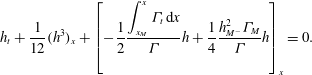 $$\begin{eqnarray}h_{t}+\frac{1}{12}(h^{3})_{x}+\left[-\frac{1}{2}\frac{\displaystyle \int _{x_{M}}^{x}{\it\Gamma}_{t}\,\text{d}x}{{\it\Gamma}}h+\frac{1}{4}\frac{h_{M^{-}}^{2}{\it\Gamma}_{M}}{{\it\Gamma}}h\right]_{x}=0.\end{eqnarray}$$
We are unable to solve (4.9) and (4.10) analytically. However, (4.9) can be considered as a quadratic equation for
 $h$
, solving which we obtain
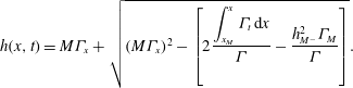 $$\begin{eqnarray}h(x,t)=M{\it\Gamma}_{x}+\sqrt{(M{\it\Gamma}_{x})^{2}-\left[2\frac{\displaystyle \int _{x_{M}}^{x}{\it\Gamma}_{t}\,\text{d}x}{{\it\Gamma}}-\frac{h_{M^{-}}^{2}{\it\Gamma}_{M}}{{\it\Gamma}}\right]}.\end{eqnarray}$$
To make some analytical progress, we assume that, near
 $x=x_{M}$
,
 ${\it\Gamma}_{t}\approx \dot{{\it\Gamma}}_{M}$
. The surfactant flux (4.9) can be approximated by
 $$\begin{eqnarray}{\textstyle \frac{1}{2}}h^{2}{\it\Gamma}-Mh{\it\Gamma}{\it\Gamma}_{x}=-\dot{{\it\Gamma}}_{M}(x-x_{M})+{\textstyle \frac{1}{2}}h_{M^{-}}^{2}{\it\Gamma}_{M}.\end{eqnarray}$$
Figure 8(a) compares the surfactant flux obtained from the numerical solution (solid lines) with the approximation in (4.12) (dashed lines) versus
 $x-x_{M}$
at
 $t=10^{5},5\times 10^{5},10^{6}$
. We observe that this linear approximation is accurate around
 $x=x_{M}$
. Further away from
 $x=x_{M}$
, this approximation breaks down, suggesting that
 ${\it\Gamma}_{t}\not\approx \dot{{\it\Gamma}}_{M}$
. This is considered in region II. Substituting
 ${\it\Gamma}_{t}\approx \dot{{\it\Gamma}}_{M}$
in (4.11) and using the compatibility condition (4.5b
), we can rewrite (4.11) as
 $$\begin{eqnarray}h(x,t)=M{\it\Gamma}_{x}+\sqrt{(M{\it\Gamma}_{x})^{2}+h_{M^{-}}^{2}\left(\frac{x-x_{M}}{x_{M}}+1\right)\frac{{\it\Gamma}_{M}}{{\it\Gamma}}}.\end{eqnarray}$$
Figure 8(b) compares the numerical solution for
 $h$
(solid lines) with its approximation in (4.13) (dashed lines) versus
 $x-x_{M}$
at
 $t=10^{5},5\times 10^{5},10^{6}$
. We use the numerical solution for
 ${\it\Gamma}$
and
 ${\it\Gamma}_{x}$
while computing the approximation for
 $h$
. We observe that (4.13) is a very good approximation for
 $h$
around
 $x=x_{M}$
. Further away from
 $x=x_{M}$
, the approximation, although overestimating
 $h$
, captures the gross behaviour, particularly the jump in
 $h$
, even though (4.12) breaks down here. This suggests that, although the flow and surfactant transport in this region are unsteady, it is the positive jump in
 ${\it\Gamma}_{x}$
that causes the positive jump in
 $h$
as shown in (4.13). It is worth noting that this region (and region II described below) has close analogies with the travelling wave structure described by Levy and co-workers (Levy & Shearer Reference Levy and Shearer2006; Levy et al.
Reference Levy, Shearer and Witelski2007) in which the fluid layer height and surfactant concentration gradient are constant on either side of
 $x=x_{M}$
when the surfactant concentration has compact support. Assuming that (4.11) admits a travelling wave solution and
 $({\it\Gamma}_{M},k_{M^{-}})\approx 0$
, we have
 $h(x,t)=h_{M^{-}}$
for
 $x<x_{M}$
and
 $h(x,t)=h_{M^{+}}=k_{M^{+}}+\sqrt{k_{M^{+}}^{2}+2s}$
for
 $x>x_{M}$
, where
 $s$
denotes the travelling wave speed. Solving the latter equation for
 $k_{M^{+}}$
, we obtain
 $k_{M^{+}}=(h_{M^{+}}^{2}-2s)/(2h_{M^{+}})$
. Writing (4.10) in travelling wave coordinates and integrating, we obtain
 $-6sh+h^{3}=12C$
, where
 $C$
is an arbitrary constant. Assuming
 $C\approx 0$
and
 $s\approx h_{M^{+}}^{2}/3$
(which is the case when the precursor thickness
 ${\it\delta}\ll 1$
), we obtain the non-zero solution
 $h_{M^{+}}=\sqrt{2}h_{M^{-}}$
. These relationships have been identified by Levy et al. (Reference Levy, Shearer and Witelski2007). The influence of the unsteady fluid flow and surfactant transport in (4.9) and (4.10) precludes any similar analytical relationships being derived for our problem.
Evolution of (a) surfactant flux
 $(h^{2}{\it\Gamma})/2-Mh{\it\Gamma}{\it\Gamma}_{x}$
and (b)
 $h$
in region C using data shown in figure 2(a,b) at the times shown. Dashed lines show the approximate solution (4.12) and (4.13) (we use the numerical solution for
 ${\it\Gamma}$
and
 ${\it\Gamma}_{x}$
at the corresponding times while computing the approximation for
 $h$
in (4.13)).

4.3. Region II
This region is part of the bulk drop in
 $x_{M^{+}}(t)\leqslant x\leqslant x_{L}(t)$
where the fluid upwells due to competing reverse Marangoni and horizontal gravity fluxes resulting in fluid accumulation and a hump-like region being formed. There is a large variation in
 ${\it\Gamma}$
from
 ${\it\Gamma}_{M}$
to
 ${\it\Gamma}_{L}$
(see figure 2
b,d),
 $h$
varies between
 $h_{M^{+}}$
and
 $h_{L^{-}}$
, and
 ${\it\Gamma}_{x}$
varies between
 $k_{M^{+}}$
and
 $k_{L^{-}}$
. Using the continuity of surfactant flux at
 $x=x_{M}$
given by (4.8), the evolution equations in this region are given by (4.9)–(4.11). We use a linear approximation for
 $$\begin{eqnarray}{\it\Gamma}_{t}\approx \left[\frac{\dot{{\it\Gamma}}_{L}-\dot{{\it\Gamma}}_{M}}{x_{L}-x_{M}}\right](x-x_{M})+\dot{{\it\Gamma}}_{M}.\end{eqnarray}$$
Substituting (4.14) in (4.9) and (4.11) gives
 $$\begin{eqnarray}\displaystyle & \displaystyle \frac{1}{2}h^{2}{\it\Gamma}-Mh{\it\Gamma}{\it\Gamma}_{x}=-\frac{1}{2}\left[\frac{\dot{{\it\Gamma}}_{L}-\dot{{\it\Gamma}}_{M}}{x_{L}-x_{M}}\right](x-x_{M})^{2}-\dot{{\it\Gamma}}_{M}(x-x_{M})+\frac{1}{2}h_{M^{-}}^{2}{\it\Gamma}_{M},\qquad & \displaystyle\end{eqnarray}$$
 $$\begin{eqnarray}\displaystyle & \displaystyle h(x,t)=M{\it\Gamma}_{x}+\sqrt{(M{\it\Gamma}_{x})^{2}-\frac{1}{{\it\Gamma}}\left[\left(\frac{\dot{{\it\Gamma}}_{L}-\dot{{\it\Gamma}}_{M}}{x_{L}-x_{M}}\right)(x-x_{M})^{2}-h_{M^{-}}^{2}{\it\Gamma}_{M}\frac{x}{x_{M}}\right]}.\qquad & \displaystyle\end{eqnarray}$$
 $x-x_{M}$
at
 $t=10^{5}$
,
 $5\times 10^{5},10^{6}$
. We observe that (4.15a
) is a much better approximation of the surfactant flux compared to the linear approximation in (4.12). Figure 9(b) compares the numerical solution for
 $h$
(solid lines) with its approximation in (4.15b
) (dashed lines) versus
 $x-x_{M}$
at
 $t=10^{5},5\times 10^{5},10^{6}$
. We use the numerical solution for
 ${\it\Gamma}$
and
 ${\it\Gamma}_{x}$
while computing the approximation for
 $h$
. Although this approximation underestimates the numerical solution, it captures the gross behaviour of the evolution of
 $h$
in this region. We again note the analogy with the work by Levy and co-workers (Levy & Shearer Reference Levy and Shearer2006; Levy et al.
Reference Levy, Shearer and Witelski2007) in which the fluid layer height and surfactant concentration gradient are constant in this region. We observe from figure 9(b) that the fluid height is not constant even at very late time, suggesting the long-lived unsteady influence of the fluid flow and surfactant transport in (4.14) and (4.15). Evaluating (4.15b
) at
 $x=x_{L}$
gives
 $$\begin{eqnarray}h_{L^{-}}=Mk_{L^{-}}+\sqrt{(Mk_{L^{-}})^{2}-\frac{1}{{\it\Gamma}_{L}}\left[(\dot{{\it\Gamma}}_{L}-\dot{{\it\Gamma}}_{M})(x_{L}-x_{M})-\frac{h_{M^{-}}^{2}x_{L}{\it\Gamma}_{M}}{x_{M}}\right]}.\end{eqnarray}$$
Evolution of (a) surfactant flux
 $(h^{2}{\it\Gamma})/2-Mh{\it\Gamma}{\it\Gamma}_{x}$
and (b)
 $h$
in region II using data shown in figure 2(a,b) at the times shown. Dashed lines show the approximate solution (4.15a,b
) (we use the numerical solution for
 ${\it\Gamma}$
and
 ${\it\Gamma}_{x}$
at the corresponding times while computing the approximation for
 $h$
in (4.15b
)).

Evolution of (a)
 $h$
and (b)
 ${\it\Gamma}$
in region A using data shown in figure 2(a,b). Dashed lines show the solution of (4.20) for
 $\hat{V}=0.18485$
,
 ${\hat{h}}_{L^{+}}=0.1$
,
 $\hat{k}_{L^{+}}=-1.797$
and
 $\hat{k}_{L^{-}}=0.3153$
(this corresponds to a particular solution curve in the family of solutions).

4.4. Region A
A thin transition region at
 $x=x_{L}(t)$
of height
 $O(h_{L^{-}})$
connects the fluid hump (region II) to the fluid front (region III). This effective contact-line region is controlled by competing surface tension, horizontal gravity and Marangoni forces. Balancing surface tension and horizontal gravity fluxes gives the width of the region to be
 $O((\mathit{Ca}\,h_{L^{-}})^{1/3})$
. Balancing convective and horizontal gravity fluxes,
 ${\dot{x}}_{L}h_{x}\sim (h^{3})_{x}$
, implies
 ${\dot{x}}_{L}\sim h_{L^{-}}^{2}$
. Balancing horizontal gravity and Marangoni fluxes implies that changes in
 ${\it\Gamma}$
across this region are of size
 $(\mathit{Ca}\,h_{L^{-}}^{4})^{1/3}/M$
and are assumed small compared to
 ${\it\Gamma}_{L}$
. We then set
 $$\begin{eqnarray}\displaystyle & \displaystyle \!x=x_{L}+(\mathit{Ca}\,h_{L^{-}})^{1/3}{\it\xi},\quad h(x,t)=h_{L^{-}}H({\it\xi}),\quad {\it\Gamma}(x,t)={\it\Gamma}_{L}+\frac{(\mathit{Ca}\,h_{L^{-}}^{4})^{1/3}}{M}G({\it\xi}),\;\qquad \; & \displaystyle\end{eqnarray}$$
 $$\begin{eqnarray}\displaystyle & \displaystyle \hat{V}=\frac{{\dot{x}}_{L}}{h_{L^{-}}^{2}},\quad {\hat{h}}_{L^{+}}=\frac{h_{L^{+}}}{h_{L^{-}}},\quad \hat{k}_{L^{-}}=\frac{Mk_{L^{-}}}{h_{L^{-}}},\quad \hat{k}_{L^{+}}=\frac{Mk_{L^{+}}}{h_{L^{-}}}.\qquad \quad & \displaystyle\end{eqnarray}$$
 $\hat{V}$
(the effective contact-line speed, representing the ratio of the advective to horizontal gravity fluxes),
 ${\hat{h}}_{L^{+}}$
(the ratio of the downstream film thickness to that upstream), and
 $\hat{k}_{L^{+}}$
and
 $\hat{k}_{L^{-}}$
(representing the ratio of the Marangoni to horizontal gravity fluxes downstream and upstream of the contact line, respectively). Assuming
 ${\it\xi}$
,
 $H$
,
 $G$
,
 $\hat{V}$
,
 ${\hat{h}}_{L^{+}}$
,
 $\hat{k}_{L^{+}}$
and
 $\hat{k}_{L^{-}}$
are all
 $O(1)$
, (2.2) reduces at leading order to
 $$\begin{eqnarray}\displaystyle & \displaystyle -\hat{V}H_{{\it\xi}}=\left[-\frac{H^{3}}{3}H_{{\it\xi}{\it\xi}{\it\xi}}+\frac{H^{2}}{2}G_{{\it\xi}}-\frac{H^{3}}{3}+\hat{D}\frac{H^{3}}{3}H_{{\it\xi}}\right]_{{\it\xi}}\!, & \displaystyle\end{eqnarray}$$
 $$\begin{eqnarray}\displaystyle & \displaystyle 0=\left[-\frac{H^{2}}{2}H_{{\it\xi}{\it\xi}{\it\xi}}+HG_{{\it\xi}}-\frac{H^{2}}{2}+\hat{D}\frac{H^{2}}{2}H_{{\it\xi}}\right]_{{\it\xi}}\!, & \displaystyle\end{eqnarray}$$
 $$\begin{eqnarray}\displaystyle & H\rightarrow 1,\quad G_{{\it\xi}}\rightarrow \hat{k}_{L^{-}}\quad \text{as}~{\it\xi}\rightarrow -\infty , & \displaystyle\end{eqnarray}$$
 $$\begin{eqnarray}\displaystyle & H\rightarrow {\hat{h}}_{L^{+}},\quad G_{{\it\xi}}\rightarrow \hat{k}_{L^{+}}\quad \text{as}~{\it\xi}\rightarrow \infty , & \displaystyle\end{eqnarray}$$
 $\hat{D}=(Dh_{L^{-}}^{2/3})/\mathit{Ca}^{1/3}$
. Equation (4.19) assumes that
 $h$
is constant far upstream and downstream, where it matches onto regions II and III, respectively. This is reasonable considering that
 $h$
in both these regions is only very weakly linear (see figure 10
a). The assumption of constant
 $h$
matching onto region III is valid only for sufficiently small values of precursor film thickness
 ${\it\delta}$
(see description of region III below). Also
 ${\it\Gamma}$
is assumed linear, matching onto regions II and III with slope
 $k_{L^{-}}~({>}0)$
and
 $k_{L^{+}}~({<}0)$
, respectively. While this matching condition is approximate for the fluid hump region, it is exact when matching onto the fluid front ahead, since
 ${\it\Gamma}$
is linear there (see region III description below). Integrating (4.18) and applying the boundary conditions (4.19), we obtain
 $$\begin{eqnarray}\displaystyle & \displaystyle H_{{\it\xi}{\it\xi}{\it\xi}}=-\left[\frac{{\hat{h}}_{L^{+}}^{2}+{\hat{h}}_{L^{+}}}{H^{3}}\right]+\left[\frac{1+{\hat{h}}_{L^{+}}+{\hat{h}}_{L^{+}}^{2}}{H^{2}}\right]+\hat{D}H_{{\it\xi}}-1, & \displaystyle\end{eqnarray}$$
 $$\begin{eqnarray}\displaystyle & \displaystyle G_{{\it\xi}}=\frac{1}{H}\left(\hat{k}_{L^{-}}-\frac{1}{2}\right)-\frac{1}{2H^{2}}({\hat{h}}_{L^{+}}+{\hat{h}}_{L^{+}}^{2})+\frac{1}{2H}(1+{\hat{h}}_{L^{+}}+{\hat{h}}_{L^{+}}^{2}). & \displaystyle\end{eqnarray}$$
 $$\begin{eqnarray}\displaystyle & \displaystyle {\dot{x}}_{L}=\frac{1}{3}\left[\frac{h_{L^{+}}^{3}-h_{L^{-}}^{3}}{h_{L^{+}}-h_{L^{-}}}\right]-\frac{M}{2}\left[\frac{h_{L^{+}}^{2}k_{L^{+}}-h_{L^{-}}^{2}k_{L^{-}}}{h_{L^{+}}-h_{L^{-}}}\right], & \displaystyle\end{eqnarray}$$
 $$\begin{eqnarray}\displaystyle & \displaystyle {\textstyle \frac{1}{2}}h_{L^{-}}^{2}-Mk_{L^{-}}h_{L^{-}}={\textstyle \frac{1}{2}}h_{L^{+}}^{2}-Mk_{L^{+}}h_{L^{+}}. & \displaystyle\end{eqnarray}$$
 $h$
in the case of only gravity-driven spreading (Troian et al.
Reference Troian, Herbolzheimer, Safran and Joanny1989; Hocking Reference Hocking1990; Bertozzi & Brenner Reference Bertozzi and Brenner1997). The effective contact-line speed
 ${\dot{x}}_{L}$
in (4.21a
) shows the competition between gravity and the Marangoni effect, with Marangoni slowing down the contact-line speed. The numerical solution of (4.20) subject to the boundary conditions in (4.19) is shown in figure 10(a,b) (dashed lines) for
 $\hat{V}=0.18485$
,
 ${\hat{h}}_{L^{+}}=0.1$
,
 $\hat{k}_{L^{+}}=-1.797$
and
 $\hat{k}_{L^{-}}=0.3153$
(the constant arising from integrating (4.20b
) is chosen such that
 $G(0)=0$
, since by definition
 ${\it\xi}=0$
is where
 $G$
has a maximum). It matches the numerical solution closely and corresponds to a particular solution curve in the family of solutions. Equation (4.20) is similar to the differential equations derived by Levy et al. (Reference Levy, Shearer and Witelski2007) for the fluid layer height and surfactant concentration assuming a travelling wave solution structure in this region. Moreover, their equations are also coupled, unlike (4.20). We assume
 ${\it\Gamma}_{t}$
to be small in this region compared to
 ${\it\Gamma}_{L}$
, which allows the equations to be decoupled. Retaining this unnecessarily complicates the equations without significantly influencing the solution structure.


4.5. Region III
This region contains the spreading fluid front in
 $x_{L}<x<x_{SL}$
of height
 $O({\it\delta})$
. The flow in this region is predominantly driven by Marangoni forces and exhibits the self-similar structure similar to that identified in Jensen & Grotberg (Reference Jensen and Grotberg1992). Balancing convective and Marangoni fluxes,
 ${\dot{x}}_{SL}h_{x}\sim (Mh^{2}{\it\Gamma}_{x})_{x}$
, implies
 ${\it\Gamma}_{x}\sim {\dot{x}}_{SL}/(M{\it\delta})$
. Hence,
 ${\it\Gamma}\sim {\dot{x}}_{SL}(x_{SL}-x_{L})/(M{\it\delta})$
(
 $x_{SL}>x_{L}$
for all
 $t$
). We set
 $$\begin{eqnarray}\displaystyle & \displaystyle x=x_{L}+(x_{SL}-x_{L}){\it\xi},\quad h(x,t)={\it\delta}H({\it\xi}),\quad {\it\Gamma}(x,t)=\frac{{\dot{x}}_{SL}(x_{SL}-x_{L})}{M{\it\delta}}\;G({\it\xi}),\qquad & \displaystyle\end{eqnarray}$$
 $$\begin{eqnarray}\displaystyle & \displaystyle {\it\gamma}=\frac{{\dot{x}}_{L}}{{\dot{x}}_{SL}},\quad {\it\alpha}=\frac{x_{SL}\ddot{x}_{SL}}{{\dot{x}}_{SL}^{2}},\quad {\it\alpha}_{1}=\frac{1-x_{L}}{x_{SL}}.\qquad & \displaystyle\end{eqnarray}$$
 $O(1/(x_{SL}-x_{L}))$
, (2.2) becomes
 $$\begin{eqnarray}\displaystyle & \displaystyle H_{{\it\xi}}[-{\it\xi}(1-{\it\gamma})-{\it\gamma}]+\left(-\frac{H^{2}}{2}G_{{\it\xi}}\right)_{{\it\xi}}=0, & \displaystyle\end{eqnarray}$$
 $$\begin{eqnarray}\displaystyle & G(1+{\it\alpha}{\it\alpha}_{1}-{\it\gamma})+G_{{\it\xi}}[-{\it\xi}(1-{\it\gamma})-{\it\gamma}]+(-HGG_{{\it\xi}})_{{\it\xi}}=0, & \displaystyle\end{eqnarray}$$
 $H=2$
and
 $G=0$
at
 ${\it\xi}=1$
(see Jensen & Grotberg Reference Jensen and Grotberg1992). Assuming
 ${\it\gamma}=1+({\it\alpha}{\it\alpha}_{1})/2$
(figure 12
a confirms this; noise in the data is due to numerical approximation in computing the derivatives involved in the relevant variables) and integrating (4.23), we obtain
 $$\begin{eqnarray}H({\it\xi})=2\left[\frac{{\it\xi}-A}{1-A}\right],\quad G({\it\xi})=-\frac{1}{2}({\it\xi}-1),\end{eqnarray}$$
where
 $A=1+2/({\it\alpha}{\it\alpha}_{1})$
. The time evolution of
 $A$
seen in figure 12(b) shows it to be large and negative, with
 $A\approx -50$
(the noise in the data is attributed to the numerical approximation in computing the derivatives involved). The dashed lines in figure 11(a,b) show
 $H$
and
 $G$
given by (4.24), which match the rescaled numerical solution very well. We note that, since
 $A$
is large and negative, so the slope of
 $h$
is small and positive, hence,
 $h\approx 2{\it\delta}$
in this region, which makes it appear to look like a ‘step’. This is true for sufficiently small values of the precursor film thickness
 ${\it\delta}$
. However, for larger values of
 ${\it\delta}$
,
 $A$
decreases in magnitude and hence the slope of this region increases and it no longer looks like a step. Hence, for sufficiently small
 ${\it\delta}$
and
 $x\rightarrow x_{L}^{+}$
, we obtain
 $$\begin{eqnarray}h_{L^{+}}=2{\it\delta},\quad {\it\Gamma}_{L}={\dot{x}}_{SL}(x_{SL}-x_{L})/(2{\it\delta}M),\quad k_{L^{+}}=-{\dot{x}}_{SL}/(2{\it\delta}M).\end{eqnarray}$$
It is worthwhile comparing (4.24) with the travelling wave solution derived by Levy & Shearer (Reference Levy and Shearer2006), where the fluid layer height and surfactant concentration gradient in this region are constant. In the travelling wave frame of reference, a balance between the convective, Marangoni and horizontal gravity fluxes admits constant solutions in fluid layer height and surfactant concentration gradient if and only if the travelling wave speed
 $s=-h_{L^{+}}k_{L^{+}}+h_{L^{+}}^{2}/2$
(the surfactant transport speed). However, in our problem the dynamics of this region is controlled by convective and Marangoni fluxes, which dominate that due to horizontal gravity. This balance admits a linear solution in the fluid height (and surfactant concentration), which distinguishes it from that derived by Levy & Shearer (Reference Levy and Shearer2006).
(a) Numerical validation of
 ${\it\gamma}=1+({\it\alpha}{\it\alpha}_{1})/2$
and (b) the time evolution of
 $A=1+2/({\it\alpha}{\it\alpha}_{1})$
, showing it to be large and negative and
 $A\approx -50$
. The noisy data are due to numerical approximation in computing the derivatives involved in the relevant variables.

4.6. Region B
The structure of the kinematic shock near
 $x=x_{SL}$
has been described in detail previously (Jensen & Grotberg Reference Jensen and Grotberg1992; Jensen Reference Jensen1994; Jensen & Halpern Reference Jensen and Halpern1998) and is not discussed here. In the parameter regime relevant here, the discontinuity in the film thickness (equal to
 $2{\it\delta}$
) is smoothed by surface tension effects and the jump in the surfactant gradient (equal to
 $k_{L^{+}}$
) is smoothed by surface diffusion (see figure 12
a,b near
 ${\it\xi}=1$
), but the region remains dynamically passive. Ahead of region C, the film in region IV is undisturbed and equals the precursor thickness.
4.7. DAE model
Equations (4.5b,c
), (4.7), (4.8), (4.16), (4.21a,b
) and (4.25a−c
) provide a system of differential–algebraic equations for the characteristic variables
 ${\it\Gamma}_{M}$
,
 $h_{T}$
,
 $x_{M}$
,
 $k_{M^{+}}$
,
 $h_{L^{-}}$
,
 $x_{L}$
,
 $k_{L^{-}}$
,
 $h_{L^{+}}$
,
 ${\it\Gamma}_{L}$
and
 $k_{L^{+}}$
, respectively. The total fluid volume and surfactant mass in the region
 $x_{T}\leqslant x<\infty$
are conserved and can be approximated as
 $$\begin{eqnarray}\displaystyle & \displaystyle \!\mathscr{V}=\!\int _{x_{T}}^{\infty }\!(h-{\it\delta})\,\text{d}x\approx \frac{2}{3}\frac{h_{M_{-}}}{\sqrt{x_{M}}}(x_{M}-x_{T})^{3/2}+\frac{1}{2}(x_{L}-x_{M})(h_{M^{+}}+h_{L^{-}})+{\it\delta}(x_{SL}+x_{T}-2x_{L}),\;\hspace{-9.60004pt} & \displaystyle \nonumber\\ \displaystyle & & \displaystyle\end{eqnarray}$$
 $$\begin{eqnarray}\displaystyle & \displaystyle \mathscr{M}=\int _{x_{T}}^{\infty }\!{\it\Gamma}\,\text{d}x\approx {\it\Gamma}_{M}(x_{M}-x_{T})+\frac{1}{2}({\it\Gamma}_{L}+{\it\Gamma}_{M})(x_{L}-x_{M})+\frac{{\dot{x}}_{SL}}{4{\it\delta}M}(x_{SL}-x_{L})^{2},\qquad & \displaystyle\end{eqnarray}$$
 $\mathscr{V}$
and
 $\mathscr{M}$
are the total fluid volume and surfactant mass, respectively. Since we do not have analytical expressions for
 $h$
and
 ${\it\Gamma}$
in region II, we approximate this region as a trapezium when evaluating the fluid volume and surfactant mass. Equation (4.26) provide equations for the characteristic variables
 $h_{M^{+}}$
and
 $x_{SL}$
, respectively. The equation for the remaining characteristic variable
 $h_{M_{-}}$
is derived as follows. Since
 $h$
in region I is similar to that due to spreading under gravity alone with no surfactant, we can use the solution for
 $h$
in (4.4) (with
 $h_{T}$
,
 $x_{T}\approx 0$
) and similarity to write
 $h_{M_{-}}/{\hat{h}}_{L}=\sqrt{x_{M}/\hat{x}_{L}}$
, where
 $\hat{x}_{L}$
and
 ${\hat{h}}_{L}$
are the location and height of the leading edge of the drop spreading under gravity alone. Equation (4.26a
) for gravity-driven spreading with no surfactant reduces to
 $\mathscr{V}=2{\hat{h}}_{L}\hat{x}_{L}/3$
. The effective contact-line speed (4.21a
) for this case reduces to
 $\dot{\hat{x}}_{L}={\hat{h}}_{L}^{2}/3$
(setting
 $M=0$
and
 $h_{L^{+}}={\it\delta}\ll {\hat{h}}_{L}$
). Solving these, we obtain
 $\hat{x}_{L}=[(9/4)\mathscr{V}^{2}(t-t_{0})+\hat{x}_{L}^{0^{3}}]^{1/3}$
and
 ${\hat{h}}_{L}=3\mathscr{V}/\{2[(9/4)\mathscr{V}^{2}(t-t_{0})+\hat{x}_{L}^{0^{3}}]^{1/3}\}$
, where
 $\hat{x}_{L}^{0}$
is the value of
 $\hat{x}_{L}$
at
 $t=t_{0}$
. Hence,
 $$\begin{eqnarray}h_{M_{-}}=\frac{3\mathscr{V}}{2}\frac{\sqrt{x_{M}}}{[\frac{9}{4}\mathscr{V}^{2}(t-t_{0})+\hat{x}_{L}^{0^{3}}]^{1/2}}.\end{eqnarray}$$
The system of DAEs are parametrised by
 $\mathscr{V}$
,
 $\mathscr{M}$
,
 $M$
and
 ${\it\delta}$
. The PDE simulations used
 $\mathscr{M}=4/3$
and
 $\mathscr{V}=2$
. Initial values for the differential equations,
 ${\it\Gamma}_{M}^{0}$
,
 $h_{T}^{0}$
,
 $x_{M}^{0}$
,
 $x_{L}^{0}$
,
 $x_{SL}^{0}$
and
 $\hat{x}_{L}^{0}$
, are fitted from the numerical solution at
 $t_{0}=10^{5}$
. These are used to determine consistent initial conditions for the algebraic equations. The DAEs are solved numerically, and their solution provides a good approximation for the behaviour in
 $t>10^{5}$
(dashed lines in figure 5
a–d). The unsteady nature of the flow and surfactant transport in regions C and II prohibits a uniformly asymptotic approximation and limits the accuracy of the predictions of
 $h_{M^{+}}$
,
 $h_{L^{-}}$
,
 $k_{M^{+}}$
and
 $k_{L^{-}}$
, but nevertheless illustrates an important feature of the spreading dynamics. Once
 $x_{M}\gg x_{T}$
, further simplification is possible:
 $h_{M_{-}}$
and
 $x_{M}$
are similar to gravity-driven spreading, so
 $h_{M_{-}}\propto {\hat{h}}_{L}\propto t^{-1/3}$
and
 $x_{M}\propto \hat{x}_{L}\propto t^{1/3}$
(Hocking Reference Hocking1990). The majority of the surfactant is contained in regions II and III and
 ${\it\Gamma}_{M}\ll {\it\Gamma}_{L}$
, so (4.26b
) can be approximated as
 $\mathscr{M}\approx {\it\Gamma}_{L}(x_{L}-x_{M})/2+{\dot{x}}_{SL}(x_{SL}-x_{L})^{2}/(4{\it\delta}M)$
. This implies
 ${\dot{x}}_{SL}(x_{SL}-x_{L})^{2}\sim 1$
and
 ${\it\Gamma}_{L}(x_{L}-x_{M})\sim 1$
, which suggests
 $x_{SL}\propto x_{L}\propto t^{1/3}$
and
 ${\it\Gamma}_{L}\propto t^{-1/3}$
(consistent with (4.25b
)). Equation (4.25c
) gives
 $k_{L^{+}}\propto {\dot{x}}_{SL}\propto t^{-2/3}$
. A balance of terms in (4.21b
) then implies that
 $h_{L_{-}}\propto k_{L^{+}}^{1/2}\propto t^{-1/3}$
and
 $k_{L^{-}}h_{L_{-}}\propto k_{L^{+}}$
, hence
 $k_{L^{-}}\propto t^{-1/3}$
. A balance of terms in (4.8) gives
 $h_{M_{+}}\propto h_{M_{-}}\propto t^{-1/3}$
and
 $k_{M^{+}}h_{M_{+}}\propto h_{M_{-}}^{2}$
, hence
 $k_{M^{+}}\propto t^{-1/3}$
. Finally, (4.5c
) gives
 $h_{T}\propto t^{-1/2}$
. These scalings are all borne out by the numerical solutions in figure 5(a–d).
5. Stability to transverse perturbations
Having captured to a reasonable level of accuracy the structure and dynamics of the spatially one-dimensional flow, we now investigate its stability to small-amplitude disturbances. Edmonstone et al. (Reference Edmonstone, Matar and Craster2004, Reference Edmonstone, Matar and Craster2005a
,Reference Edmonstone, Matar and Craster
b
), using transient growth analysis of the entire time-dependent flow, showed that growing disturbances are initially confined to the neighbourhood of the drop’s leading-edge contact line. We therefore focus on region A, perturbing the quasi-steady solution satisfying (4.20), looking for disturbances with transverse wavenumber
 $q^{\star }$
. By treating the base state as quasi-steady during the evolution of disturbances, its weak algebraic time dependence is captured parametrically through
 $\hat{V}$
,
 ${\hat{h}}_{L^{+}}$
,
 $\hat{k}_{L^{+}}$
and
 $\hat{k}_{L^{-}}$
. We reduce this dependence to two parameters
 ${\hat{h}}_{L^{+}}$
and
 $\hat{k}_{L^{+}}$
using the relations in (4.21).
The scaling (4.17a
) with
 $y=(\mathit{Ca}\,h_{L^{-}})^{1/3}{\it\eta}$
and
 $t=(\mathit{Ca}\,h_{L^{-}}^{-5})^{1/3}{\it\tau}$
reduces (2.1) in region A (neglecting surfactant diffusion) to
 $$\begin{eqnarray}\displaystyle & \displaystyle H_{{\it\tau}}-\hat{V}H_{{\it\xi}}=\hat{\boldsymbol{{\rm\nabla}}}\boldsymbol{\cdot }\left(-\frac{H^{3}}{3}\hat{\boldsymbol{{\rm\nabla}}}\hat{{\rm\nabla}}^{2}H+\frac{H^{2}}{2}\hat{\boldsymbol{{\rm\nabla}}}G+\hat{D}({\it\theta})\frac{H^{3}}{3}\hat{\boldsymbol{{\rm\nabla}}}H\right)-\left(\frac{H^{3}}{3}\right)_{{\it\xi}}, & \displaystyle\end{eqnarray}$$
 $$\begin{eqnarray}\displaystyle & \displaystyle 0=\hat{\boldsymbol{{\rm\nabla}}}\boldsymbol{\cdot }\left(-\frac{H^{2}}{2}\hat{\boldsymbol{{\rm\nabla}}}\hat{{\rm\nabla}}^{2}H+H\hat{\boldsymbol{{\rm\nabla}}}G+\hat{D}({\it\theta})\frac{H^{2}}{2}\hat{\boldsymbol{{\rm\nabla}}}H\right)-\left(\frac{H^{2}}{2}\right)_{{\it\xi}}, & \displaystyle\end{eqnarray}$$
 $\hat{\boldsymbol{{\rm\nabla}}}=(\partial /\partial {\it\xi},\partial /\partial {\it\eta})$
. We set
 $[H({\it\xi},{\it\eta},{\it\tau}),G({\it\xi},{\it\eta},{\it\tau})]=[H_{s}({\it\xi}),G_{s}({\it\xi})]+{\it\epsilon}[{\hat{H}}({\it\xi}),{\hat{G}}({\it\xi})]\text{e}^{\text{i}q{\it\eta}}$
, where
 $[H_{s}({\it\xi}),G_{s}({\it\xi})]$
denote the quasi-steady base state for
 $h$
and
 ${\it\Gamma}$
, respectively, and
 $q=(\mathit{Ca}\,h_{L^{-}})^{1/3}q^{\star }$
is the scaled wavenumber. We recover at leading order in
 ${\it\epsilon}\ll 1$
the quasi-steady solution (4.18) (now denoted with a subscript
 $s$
). The linearised unsteady disturbances satisfy
 $$\begin{eqnarray}\displaystyle {\hat{H}}_{{\it\tau}}-\hat{V}{\hat{H}}_{{\it\xi}} & = & \displaystyle \left[\frac{H_{s}^{2}}{2}{\hat{G}}_{{\it\xi}}+H_{s}{\hat{H}}G_{s{\it\xi}}-\frac{H_{s}^{3}}{3}\left(\frac{\partial ^{2}}{\partial {\it\xi}^{2}}-q^{2}\right){\hat{H}}_{{\it\xi}}-H_{s}^{2}{\hat{H}}H_{s{\it\xi}{\it\xi}{\it\xi}}+\hat{D}({\it\theta})\frac{H_{s}^{3}}{3}{\hat{H}}_{{\it\xi}}\right]_{{\it\xi}}\nonumber\\ \displaystyle & & \displaystyle +\,[\hat{D}({\it\theta})H_{s}^{2}{\hat{H}}_{1}H_{s{\it\xi}}]_{{\it\xi}}-q^{2}\frac{H_{s}^{2}}{2}{\hat{G}}+q^{2}\frac{H_{s}^{3}}{3}\left(\frac{\partial ^{2}}{\partial {\it\xi}^{2}}-q^{2}\right){\hat{H}}-(H_{s}^{2}{\hat{H}})_{{\it\xi}}\nonumber\\ \displaystyle & & \displaystyle -\,q^{2}\hat{D}({\it\theta})\frac{H_{s}^{3}}{3}{\hat{H}},\end{eqnarray}$$
 $$\begin{eqnarray}\displaystyle 0 & = & \displaystyle \left[H_{s}{\hat{G}}_{{\it\xi}}+{\hat{H}}G_{s{\it\xi}}-\frac{H_{s}^{2}}{2}\left(\frac{\partial ^{2}}{\partial {\it\xi}^{2}}-q^{2}\right){\hat{H}}_{{\it\xi}}-H_{s}{\hat{H}}H_{s{\it\xi}{\it\xi}{\it\xi}}+\hat{D}({\it\theta})\frac{H_{s}^{2}}{2}{\hat{H}}_{{\it\xi}}\right]_{{\it\xi}}\nonumber\\ \displaystyle & & \displaystyle +\,[\hat{D}({\it\theta})H_{s}{\hat{H}}H_{s{\it\xi}}]_{{\it\xi}}-q^{2}H_{s}{\hat{G}}+q^{2}\frac{H_{s}^{2}}{2}\left(\frac{\partial ^{2}}{\partial {\it\xi}^{2}}-q^{2}\right){\hat{H}}-(H_{s}{\hat{H}})_{{\it\xi}}\nonumber\\ \displaystyle & & \displaystyle -\,q^{2}\hat{D}({\it\theta})\frac{H_{s}}{2}{\hat{H}},\end{eqnarray}$$
Solutions of (5.2) for
 $q=0.3$
,
 ${\it\theta}=90^{\circ }$
(solid lines) using a base state (dashed lines) evaluated at
 $t=2\times 10^{5}$
(
 ${\hat{h}}_{L^{+}}=0.0884$
and
 $\hat{k}_{L^{+}}=-2$
). Arrows show time increasing between
 $t=10$
and 100.

Late-time growth rate
 ${\it\beta}$
versus wavenumber
 $q$
: (a) for
 ${\it\theta}=90^{\circ }$
and base states evaluated at times
 $t=10^{4}$
,
 $10^{5}$
,
 $2\times 10^{5}$
,
 $5\times 10^{5}$
and
 $10^{6}$
; (b) for inclination angles
 ${\it\theta}=90^{\circ }$
, 60° and 3° for base state corresponding to
 ${\hat{h}}_{L^{+}}=0.0884$
and
 $\hat{k}_{L^{+}}=-2$
(corresponding to time
 $t=2\times 10^{5}$
); and (c) comparison of gravity-driven (dashed line) and surfactant and gravity-driven (solid line) spreading for
 ${\it\theta}=90^{\circ }$
(corresponding to a base state with
 ${\hat{h}}_{L^{+}}=0.0884$
and
 $\hat{k}_{L^{+}}=-2$
).

subject to
 $({\hat{H}},{\hat{G}})\rightarrow 0$
as
 ${\it\xi}\rightarrow \pm \infty$
. We solved (5.2) numerically by time stepping, using a uniform finite difference grid on a domain
 $-20\leqslant {\it\xi}\leqslant 20$
, tracking the evolution of localised disturbances (initially
 ${\hat{H}}={\hat{G}}=10^{-3}\exp (-10{\it\xi}^{2})$
). The evolution depends on the wavenumber
 $q$
,
 $\hat{D}$
(related to the inclination angle) and parameters
 ${\hat{h}}_{L^{+}}$
and
 $\hat{k}_{L^{+}}$
(characterising the quasi-steady base state
 $H_{s}$
and
 $G_{s}$
). Figure 13(a,b) shows the evolution of
 ${\hat{H}}$
and
 ${\hat{G}}$
(solid lines), respectively, for
 $q=0.3$
and
 $\hat{D}=0$
(corresponding to
 ${\it\theta}=90^{\circ }$
) emanating from a base state (dashed lines) evaluated at
 $t=2\times 10^{5}$
(corresponding to
 ${\hat{h}}_{L^{+}}=0.0884$
and
 $\hat{k}_{L^{+}}=-2$
). It is observed that, under suitable conditions, disturbances can grow rapidly: perturbations to
 ${\hat{H}}$
and
 ${\hat{G}}$
are larger near the effective contact line, features identified previously by Edmonstone et al. (Reference Edmonstone, Matar and Craster2005b
). It is also noted for future reference that
 ${\hat{G}}$
is minimum where
 ${\hat{H}}$
is maximum and vice versa. At late times (for
 ${\it\tau}\geqslant 50$
), the growth of disturbances is approximately exponential, with
 ${\hat{H}},{\hat{G}}\propto \exp ({\it\beta}{\it\tau})$
, where
 ${\it\beta}$
is the growth rate. The computed growth rate
 ${\it\beta}$
is shown in figure 14(a) as a function of the wavenumber
 $q$
for
 ${\it\theta}=90^{\circ }$
and base states evaluated at times ranging between
 $t=10^{4}$
and
 $10^{6}$
. The shape of the dispersion relation resembles that obtained by Edmonstone et al. (Reference Edmonstone, Matar and Craster2005b
) using their transient growth analysis. For small values of
 $q$
, growing disturbances ultimately reached the boundaries of the domain; growth rates were then sensitive to the size of the domain chosen. This prevented us from computing reliable solutions for
 $q<0.1$
. However, the simulations demonstrate convincingly that the most linearly unstable mode has wavenumber comparable to the width of region A, that, as time increases, the base state becomes less linearly unstable (as seen in figure 14(a), where the maximum growth rate and band of unstable wavenumbers decrease as
 $t$
increases), and that sufficiently short-wavelength disturbances are linearly stable. Figure 14(b) shows the dispersion relation for varying inclination angles
 ${\it\theta}=3^{\circ }$
, 60°, 90° for base state corresponding to
 ${\hat{h}}_{L^{+}}=0.0884$
and
 $\hat{k}_{L^{+}}=-2$
. It is observed that decreasing the inclination angle has a stabilising effect, with both the maximum growth rate and the bandwidth of unstable wavenumbers decreasing, in agreement with the transient growth analysis by Edmonstone et al. (Reference Edmonstone, Matar and Craster2005b
). Finally, we compare the dispersion relation between surfactant and gravity-driven spreading and gravity-driven spreading alone by showing in figure 14(c) the dispersion relation computed for the latter case (by setting
 $G_{s}={\hat{G}}=0$
in (5.2a
) and using the same procedure as described above for extracting the growth rate). The inclination angle
 ${\it\theta}=90^{\circ }$
and the base states for
 $H_{s}$
and
 $G_{s}$
correspond to
 ${\hat{h}}_{L^{+}}=0.0884$
and
 $\hat{k}_{L^{+}}=-2$
. We observe that the growth rate and band of unstable wavenumbers are smaller for the gravity-driven case, indicating the additional destabilising contribution due to surfactant. Moreover, at small wavenumbers, the dispersion relation is markedly different, with quadratic behaviour for gravity-driven spreading (Troian et al.
Reference Troian, Herbolzheimer, Safran and Joanny1989; Bertozzi & Brenner Reference Bertozzi and Brenner1997) and linear for surfactant and gravity-driven spreading. Furthermore, it can be shown that for gravity-driven spreading there is a critical inclination angle
 ${\it\theta}$
below which the base state is linearly stable for all wavenumbers, in contrast to surfactant and gravity-driven spreading, where it was speculated to be linearly unstable for all angles by Edmonstone et al. (Reference Edmonstone, Matar and Craster2005b
). These are analysed in more detail in the next section by performing a small-wavenumber (or long-wavelength) analysis about the base state, which forms part of the discrete spectrum of the linear operator in (5.2).
5.1. Small-wavenumber analysis
In this section we examine instabilities with wavelength intermediate between the width of region A and regions II and III, and assume exponential time dependence so that
 ${\hat{H}}_{{\it\tau}}$
in (5.2a
) becomes
 ${\it\beta}{\hat{H}}$
. Numerical dispersion relations (see figure 14) suggest that the growth rate is linear at small wavenumbers, so we write
 $[{\hat{H}},{\hat{G}},{\it\beta}]=[H,G,{\it\beta}]_{0}+q[H,G,{\it\beta}]_{1}+q^{2}[H,G,{\it\beta}]_{2}+\cdots \,$
. Substituting in (5.2), at leading order in
 $q$
, we obtain
 $(H_{0},G_{0})=(-H_{s{\it\xi}},-G_{s{\it\xi}})$
and
 ${\it\beta}_{0}=0$
, which represents a translation of the base state
 $(H_{s},G_{s})$
. At
 $O(q)$
, we obtain
 $$\begin{eqnarray}\displaystyle -\!{\it\beta}_{1}H_{s{\it\xi}}-\hat{V}H_{1{\it\xi}} & = & \displaystyle \left[\frac{H_{s}^{2}}{2}G_{1{\it\xi}}+H_{s}G_{s{\it\xi}}H_{1}-\frac{H_{s}^{3}}{3}H_{1{\it\xi}{\it\xi}{\it\xi}}-H_{s}^{2}H_{s{\it\xi}{\it\xi}{\it\xi}}H_{1}+\hat{D}({\it\theta})\frac{H_{s}^{3}}{3}H_{1{\it\xi}}\right.\nonumber\\ \displaystyle & & \displaystyle +\left.\vphantom{\frac{H_{s}^{2}}{2}}\hat{D}({\it\theta})H_{s}^{2}H_{s{\it\xi}}H_{1}-H_{s}^{2}H_{1}\right]_{{\it\xi}}\!,\end{eqnarray}$$
 $$\begin{eqnarray}0=\left[H_{s}G_{1{\it\xi}}+H_{1}G_{s{\it\xi}}-\frac{H_{s}^{2}}{2}H_{1{\it\xi}{\it\xi}{\it\xi}}H_{1}+\hat{D}({\it\theta})\frac{H_{s}^{2}}{2}H_{1{\it\xi}}+\hat{D}({\it\theta})H_{s}H_{s{\it\xi}}H_{1}-H_{s}H_{1}\right]_{{\it\xi}}\!.\end{eqnarray}$$
 $H_{1}$
and all its derivatives decay to zero as
 ${\it\xi}\rightarrow \pm \infty$
and
 $G_{1{\it\xi}}$
tends to a constant
 $A$
as
 ${\it\xi}\rightarrow \infty$
and
 $G_{1{\it\xi}}$
tends to a constant
 $B$
as
 ${\it\xi}\rightarrow -\infty$
. The last two conditions are required to balance the unsteady and the Marangoni terms (first and third terms) in (5.3a
) and are also motivated in part by the fact that the leading-order solution
 $G_{0}$
tends to a constant value
 $-\hat{k}_{L^{-}}$
and
 $-\hat{k}_{L^{+}}$
as
 ${\it\xi}\rightarrow -\infty$
,
 $\infty$
, respectively. Using
 $H_{s}\rightarrow {\hat{h}}_{L^{+}}$
,
 $G_{s{\it\xi}}\rightarrow \hat{k}_{L^{+}}$
,
 $H_{s{\it\xi}},H_{s{\it\xi}{\it\xi}{\it\xi}}\rightarrow 0$
as
 ${\it\xi}\rightarrow \infty$
and
 $H_{s}\rightarrow 1$
,
 $G_{s{\it\xi}}\rightarrow \hat{k}_{L^{-}}$
,
 $H_{s{\it\xi}},H_{s{\it\xi}{\it\xi}{\it\xi}}\rightarrow 0$
as
 ${\it\xi}\rightarrow -\infty$
, we obtain the following conditions after integrating (5.3) between
 $-\infty$
and
 $\infty$
:
 $$\begin{eqnarray}{\it\beta}_{1}=\left[\frac{{\textstyle \frac{1}{2}}A{\hat{h}}_{L^{+}}^{2}-{\textstyle \frac{1}{2}}B}{1-{\hat{h}}_{L^{+}}}\right],\quad B=A{\hat{h}}_{L^{+}}\quad \Longrightarrow \quad {\it\beta}_{1}=-B/2=-A{\hat{h}}_{L^{+}}/2.\end{eqnarray}$$
To determine the growth rate
 ${\it\beta}_{1}$
, we need to determine either
 $A$
or
 $B$
, which is done as follows. When
 $q\ll 1$
, we assume that
 ${\hat{H}}$
and
 ${\hat{G}}$
have a three-region structure: an inner region near the drop’s contact line in which
 ${\it\xi}=O(1)$
and
 ${\hat{H}}=-H_{s{\it\xi}}$
,
 ${\hat{G}}=-G_{s{\it\xi}}$
to leading order, and two outer regions of length scales
 $O(1/q)$
. We suppose that the drop’s contact line (when viewed from the outer regions) lies along
 ${\it\xi}={\it\epsilon}\exp (\text{i}q{\it\eta}+{\it\beta}{\it\tau})$
, so that to leading order, at the outer limits of the inner region, we have
 $$\begin{eqnarray}G\sim \hat{k}_{L^{-}}[{\it\xi}-{\it\epsilon}\exp (\text{i}q{\it\eta}+{\it\beta}{\it\tau})]\quad ({\it\xi}\rightarrow -\infty ),\quad G\sim \hat{k}_{L^{+}}[{\it\xi}-{\it\epsilon}\exp (\text{i}q{\it\eta}+{\it\beta}{\it\tau})]\quad ({\it\xi}\rightarrow \infty ).\end{eqnarray}$$
We now show how perturbations to
 $G$
affect the surfactant gradient
 ${\hat{G}}_{{\it\xi}}$
ahead of and behind the contact line.
To describe the outer regions, we rescale with
 ${\it\xi}=z/q$
,
 ${\hat{G}}=\tilde{G}/q$
,
 ${\it\beta}=q\tilde{{\it\beta}}$
(anticipating
 $\tilde{{\it\beta}}=O(1)$
), so that (5.2) becomes (after dividing by
 $q$
)
 $$\begin{eqnarray}\displaystyle \tilde{{\it\beta}}{\hat{H}}-\hat{V}{\hat{H}}_{z} & = & \displaystyle \left[\frac{H_{s}^{2}}{2}\tilde{G}_{z}+H_{s}G_{s{\it\xi}}{\hat{H}}-q^{3}\frac{H_{s}^{3}}{3}\left(\frac{\partial ^{2}}{\partial z^{2}}-1\right){\hat{H}}_{z}-H_{s}^{2}H_{s{\it\xi}{\it\xi}{\it\xi}}{\hat{H}}+q\hat{D}({\it\theta})\frac{H_{s}^{3}}{3}{\hat{H}}_{z}\right.\nonumber\\ \displaystyle & & \displaystyle \left.+\,\vphantom{\frac{H_{s}^{2}}{2}}\hat{D}({\it\theta})H_{s}^{2}H_{s{\it\xi}}{\hat{H}}\right]_{z}-\frac{H_{s}^{2}}{2}\tilde{G}+q^{3}\frac{H_{s}^{3}}{3}\left(\frac{\partial ^{2}}{\partial z^{2}}-1\right){\hat{H}}-(H_{s}^{2}{\hat{H}})_{z}\nonumber\\ \displaystyle & & \displaystyle -\,q\hat{D}({\it\theta})\frac{H_{s}^{3}}{3}{\hat{H}},\end{eqnarray}$$
 $$\begin{eqnarray}\displaystyle 0 & = & \displaystyle \left[H_{s}\tilde{G}_{z}+{\hat{H}}G_{s{\it\xi}}-q^{3}\frac{H_{s}^{2}}{2}\left(\frac{\partial ^{2}}{\partial z^{2}}-1\right){\hat{H}}_{z}-H_{s}H_{s{\it\xi}{\it\xi}{\it\xi}}{\hat{H}}+q\hat{D}({\it\theta})\frac{H_{s}^{2}}{2}{\hat{H}}_{z}\right.\nonumber\\ \displaystyle & & \displaystyle \left.+\,\vphantom{\frac{H_{s}^{2}}{2}}\hat{D}({\it\theta})H_{s}H_{s{\it\xi}}{\hat{H}}\right]_{z}-H_{s}\tilde{G}+q^{3}\frac{H_{s}^{2}}{2}\left(\frac{\partial ^{2}}{\partial z^{2}}-1\right){\hat{H}}-(H_{s}{\hat{H}})_{z}\nonumber\\ \displaystyle & & \displaystyle -\,q\hat{D}({\it\theta})\frac{H_{s}^{2}}{2}{\hat{H}}.\end{eqnarray}$$
 $q$
as
 $z\rightarrow \infty$
, we can write (5.6) as
 $$\begin{eqnarray}\displaystyle & \displaystyle \tilde{{\it\beta}}{\hat{H}}-\hat{V}{\hat{H}}_{z}=\left[\frac{{\hat{h}}_{L^{+}}^{2}}{2}\tilde{G}_{z}+{\hat{h}}_{L^{+}}\hat{k}_{L^{+}}{\hat{H}}\right]_{z}-\frac{{\hat{h}}_{L^{+}}^{2}}{2}\tilde{G}-{\hat{h}}_{L^{+}}^{2}{\hat{H}}_{z}, & \displaystyle\end{eqnarray}$$
 $$\begin{eqnarray}\displaystyle & \displaystyle 0=[{\hat{h}}_{L^{+}}\tilde{G}_{z}+\hat{k}_{L^{+}}{\hat{H}}]_{z}-{\hat{h}}_{L^{+}}\tilde{G}-{\hat{h}}_{L^{+}}{\hat{H}}_{z}, & \displaystyle\end{eqnarray}$$
 $$\begin{eqnarray}{\hat{H}}_{z}-\frac{\tilde{{\it\beta}}}{{\it\alpha}}{\hat{H}}=0,\quad \tilde{G}_{zz}-\tilde{G}=\left(1-\frac{\hat{k}_{L^{+}}}{{\hat{h}}_{L^{+}}}\right){\hat{H}}_{z},\end{eqnarray}$$
where
 ${\it\alpha}=[({\hat{h}}_{L^{+}}^{2}/2)+({\hat{h}}_{L^{+}}\hat{k}_{L^{+}}/2)-{\hat{h}}_{L^{+}}^{2}+\hat{V}]$
. Thus
 ${\hat{H}}={\hat{H}}_{0}\exp (\tilde{{\it\beta}}z/{\it\alpha})$
for some
 ${\hat{H}}_{0}$
. For
 $\tilde{{\it\beta}}>0$
and
 ${\it\alpha}>0$
(observed numerically), we require
 $\tilde{H}_{0}=0$
for perturbations to remain bounded as
 $z\rightarrow \infty$
(the contact line moves faster than any growing disturbances to the fluid front ahead). Thus
 $\tilde{G}=\tilde{G}_{0}\exp (-z)$
as
 $z\rightarrow \infty$
for some
 $\tilde{G}_{0}$
. To match with (5.5b
) we take
 $\tilde{G}_{0}=-q\hat{k}_{L^{+}}$
. Thus towards the contact line as
 $z\rightarrow 0^{+}$
,
 ${\hat{H}}=0$
and
 $$\begin{eqnarray}{\hat{G}}\sim \hat{k}_{L^{+}}(-1+q{\it\xi}-{\textstyle \frac{1}{2}}q^{2}{\it\xi}^{2}+\cdots \,).\end{eqnarray}$$
Hence, as
 ${\it\xi}\rightarrow \infty$
,
 $G_{1{\it\xi}}\rightarrow A=\hat{k}_{L^{+}}$
. Similarly, (5.6) at leading order in
 $q$
as
 $z\rightarrow -\infty$
can be written as
 $$\begin{eqnarray}\displaystyle & \tilde{{\it\beta}}{\hat{H}}-\hat{V}{\hat{H}}_{z}=[{\textstyle \frac{1}{2}}\tilde{G}_{z}+\hat{k}_{L^{-}}{\hat{H}}]_{z}-{\textstyle \frac{1}{2}}\tilde{G}-{\hat{H}}_{z}, & \displaystyle\end{eqnarray}$$
 $$\begin{eqnarray}\displaystyle & 0=[\tilde{G}_{z}+\hat{k}_{L^{-}}{\hat{H}}]_{z}-\tilde{G}-{\hat{H}}_{z}, & \displaystyle\end{eqnarray}$$
 $$\begin{eqnarray}{\hat{H}}_{z}-\frac{\tilde{{\it\beta}}}{{\it\alpha}_{1}}{\hat{H}}=0,\quad \tilde{G}_{zz}-\tilde{G}=(1-\hat{k}_{L^{-}}){\hat{H}}_{z},\end{eqnarray}$$
where
 ${\it\alpha}_{1}=[(1/2)+(\hat{k}_{L^{-}}/2)-1+\hat{V}]$
. Thus
 ${\hat{H}}={\hat{H}}_{0}\exp (\tilde{{\it\beta}}z/{\it\alpha}_{1})$
for some
 ${\hat{H}}_{0}$
. For
 $\tilde{{\it\beta}}>0$
and
 ${\it\alpha}_{1}<0$
(observed numerically), we require
 $\tilde{H}_{0}=0$
for perturbations to remain bounded as
 $z\rightarrow -\infty$
. Thus
 $\tilde{G}=\tilde{G}_{0}\exp (z)$
as
 $z\rightarrow -\infty$
for some
 $\tilde{G}_{0}$
. To match with (5.5a
) we take
 $\tilde{G}_{0}=-q\hat{k}_{L^{-}}$
. Thus towards the contact line as
 $z\rightarrow 0^{-}$
,
 ${\hat{H}}=0$
and
 $$\begin{eqnarray}{\hat{G}}\sim \hat{k}_{L^{-}}(-1-q{\it\xi}-{\textstyle \frac{1}{2}}q^{2}{\it\xi}^{2}+\cdots \,).\end{eqnarray}$$
Hence, as
 ${\it\xi}\rightarrow -\infty$
,
 $G_{1{\it\xi}}\rightarrow B=-\hat{k}_{L^{-}}$
. Using (5.4a
) we obtain the
 $O(q)$
growth rate,
 $$\begin{eqnarray}{\it\beta}_{1}=\left[\frac{{\textstyle \frac{1}{2}}\hat{k}_{L^{+}}{\hat{h}}_{L^{+}}^{2}+{\textstyle \frac{1}{2}}\hat{k}_{L^{-}}}{1-{\hat{h}}_{L^{+}}}\right].\end{eqnarray}$$
Numerical validation of the relationships (a)
 $\hat{k}_{L^{-}}=-\hat{k}_{L^{+}}{\hat{h}}_{L^{+}}$
, (b)
 $\hat{k}_{L^{-}}=(1-{\hat{h}}_{L^{+}}^{2})/4$
and (c)
 $\hat{k}_{L^{+}}=-(1-{\hat{h}}_{L^{+}}^{2})/(4{\hat{h}}_{L^{+}})$
.

Noting that
 $\hat{k}_{L^{-}}>0$
,
 $\hat{k}_{L^{+}}<0$
and
 ${\hat{h}}_{L^{+}}<1$
, the growth rate
 ${\it\beta}_{1}>0$
if
 $\hat{k}_{L^{-}}/2>-\hat{k}_{L^{+}}{\hat{h}}_{L^{+}}^{2}/2$
, i.e. the
 $O(q)$
Marangoni flux behind the contact line dominates that ahead of the contact line. If this condition is satisfied, a mechanism for the flow to become linearly unstable at
 $O(q)$
is due to the forward Marangoni flux behind the contact line pulling more fluid into the contact-line region than the forward Marangoni flux ahead of the contact line dragging fluid out. This results in growth of perturbations in
 $h$
, consequently destabilising the flow and the contact line (consistent with figure 13, where
 ${\hat{H}}$
is positive and growing immediately behind the contact line, coinciding with
 ${\hat{G}}_{{\it\xi}}$
, which is negative there). We now verify whether the above condition is satisfied. Using (5.4b
) implies
 $\hat{k}_{L^{-}}=-\hat{k}_{L^{+}}{\hat{h}}_{L^{+}}$
(figure 15
a shows that this relationship is approximately satisfied; the slight difference is due to the ambiguity in determining
 $k_{L^{-}}$
from the numerical solution), using which the above condition can be rewritten as
 $\hat{k}_{L^{-}}(1-{\hat{h}}_{L^{+}}^{2})>0$
, which is always satisfied. We also know using (4.21b
) that
 $\hat{k}_{L^{-}}=(1-{\hat{h}}_{L^{+}}^{2})/2+{\hat{h}}_{L^{+}}\hat{k}_{L^{+}}$
, which, when combined with the above relationship, gives
 $\hat{k}_{L^{-}}=(1-{\hat{h}}_{L^{+}}^{2})/4$
and
 $\hat{k}_{L^{+}}=-(1-{\hat{h}}_{L^{+}}^{2})/(4{\hat{h}}_{L^{+}})$
(figure 15
b,c shows that these relationships are approximately satisfied; the slight difference in figure 15
b is due to the ambiguity in determining
 $k_{L^{-}}$
from the numerical solution). Equation (5.13) can now be rewritten as
 $$\begin{eqnarray}{\it\beta}_{1}=\frac{1-{\hat{h}}_{L^{+}}^{2}}{8}\approx \frac{1}{8}\quad (\text{since}~{\hat{h}}_{L^{+}}\ll 1).\end{eqnarray}$$
Equation (5.14) shows that the
 $O(q)$
growth rate is always positive and independent of the angle of inclination. This suggests that the flow is linearly unstable for all angles of inclination, at least those within the validity of our model. This supports the speculation by Edmonstone et al. (Reference Edmonstone, Matar and Craster2005b
). We also note from numerics that
 ${\hat{h}}_{L^{+}}$
increases gradually with time, so
 ${\it\beta}_{1}$
decreases, confirming the observation in figure 14(a) that, as time increases, the base state becomes less linearly unstable. The analysis also shows the Marangoni effect to be dominant at this order, with gravity having no influence. Figure 16(a,b) shows the
 $O(q)$
approximation
 ${\it\beta}\approx q/8$
(dashed lines) along with the numerical dispersion relation (solid lines) for inclination angles
 ${\it\theta}=90^{\circ }$
and 3°, respectively. We observe that this approximation slightly underestimates the numerical dispersion relation for
 ${\it\theta}=90^{\circ }$
and overestimates it for
 ${\it\theta}=3^{\circ }$
.
We now determine the
 $O(q^{2})$
growth rate
 ${\it\beta}_{2}$
. At
 $O(q^{2})$
we obtain
 $$\begin{eqnarray}\displaystyle & & \displaystyle {\it\beta}_{0}H_{2}+{\it\beta}_{1}H_{1}+{\it\beta}_{2}H_{0}-\hat{V}H_{2{\it\xi}}\nonumber\\ \displaystyle & & \displaystyle \quad =\left[\frac{H_{s}^{2}}{2}G_{2{\it\xi}}+H_{s}G_{s{\it\xi}}H_{2}+\frac{H_{s}^{3}}{3}H_{0{\it\xi}}-\frac{H_{s}^{3}}{3}H_{2{\it\xi}{\it\xi}{\it\xi}}-H_{s}^{2}H_{s{\it\xi}{\it\xi}{\it\xi}}H_{2}\right]_{{\it\xi}}\nonumber\\ \displaystyle & & \displaystyle \qquad +\,\left[\hat{D}({\it\theta})\frac{H_{s}^{3}}{3}H_{2{\it\xi}}+\hat{D}({\it\theta})H_{s}^{2}H_{s{\it\xi}}H_{2}\right]_{{\it\xi}}-\frac{H_{s}^{2}}{2}G_{0}+\frac{H_{s}^{3}}{3}H_{0{\it\xi}{\it\xi}}\nonumber\\ \displaystyle & & \displaystyle \qquad -\,(H_{s}^{2}H_{2})_{{\it\xi}}-\hat{D}({\it\theta})\frac{H_{s}^{3}}{3}H_{0},\end{eqnarray}$$
 $$\begin{eqnarray}\displaystyle 0 & = & \displaystyle \left[H_{s}G_{2{\it\xi}}+G_{s{\it\xi}}H_{2}-\frac{H_{s}^{2}}{2}H_{2{\it\xi}{\it\xi}{\it\xi}}+\frac{H_{s}^{2}}{2}H_{0{\it\xi}}-H_{s}H_{s{\it\xi}{\it\xi}{\it\xi}}H_{2}\right]_{{\it\xi}}\nonumber\\ \displaystyle & & \displaystyle +\,\left[\hat{D}({\it\theta})\frac{H_{s}^{2}}{2}H_{2{\it\xi}}+\hat{D}({\it\theta})H_{s}H_{s{\it\xi}}H_{2}\right]_{{\it\xi}}-H_{s}G_{0}+\frac{H_{s}^{2}}{2}H_{0{\it\xi}{\it\xi}}\nonumber\\ \displaystyle & & \displaystyle -\,(H_{s}H_{2})_{{\it\xi}}-\hat{D}({\it\theta})\frac{H_{s}^{2}}{2}H_{0}.\end{eqnarray}$$
 $H_{1}$
,
 $H_{2}$
and their derivatives decay to zero as
 ${\it\xi}\rightarrow \pm \infty$
. Equations (5.9) and (5.12) suggest that
 $G_{2{\it\xi}}\rightarrow -\hat{k}_{L^{+}}{\it\xi}$
as
 ${\it\xi}\rightarrow \infty$
and
 $G_{2{\it\xi}}\rightarrow -\hat{k}_{L^{-}}{\it\xi}$
as
 ${\it\xi}\rightarrow -\infty$
, respectively. Using
 $H_{s}\rightarrow {\hat{h}}_{L^{+}}$
,
 $G_{s{\it\xi}}\rightarrow \hat{k}_{L^{+}}$
,
 $H_{s{\it\xi}},H_{s{\it\xi}{\it\xi}{\it\xi}}\rightarrow 0$
as
 ${\it\xi}\rightarrow \infty$
,
 $H_{s}\rightarrow 1$
,
 $G_{s{\it\xi}}\rightarrow \hat{k}_{L^{-}}$
,
 $H_{s{\it\xi}},H_{s{\it\xi}{\it\xi}{\it\xi}}\rightarrow 0$
as
 ${\it\xi}\rightarrow -\infty$
,
 $H_{0}=-H_{s,{\it\xi}}$
,
 $G_{0}=-G_{s{\it\xi}}$
and
 ${\it\beta}_{0}=0$
, we obtain the following condition after integrating (5.15a
) between
 $-\infty$
and
 $\infty$
:
 $$\begin{eqnarray}\displaystyle (1-{\hat{h}}_{L^{+}}){\it\beta}_{2} & = & \displaystyle \!\left.-\frac{1}{2}{\hat{h}}_{L^{+}}^{2}\hat{k}_{L^{+}}{\it\xi}\right|_{{\it\xi}\rightarrow \infty }+\left.\frac{1}{2}\hat{k}_{L^{-}}{\it\xi}\right|_{{\it\xi}\rightarrow -\infty }+\int _{-\infty }^{\infty }\frac{1}{2}H_{s}^{2}G_{s_{{\it\xi}}}\,\text{d}{\it\xi}\nonumber\\ \displaystyle & & \displaystyle -\int _{-\infty }^{\infty }\frac{H_{s}^{3}}{3}H_{s_{{\it\xi}{\it\xi}{\it\xi}}}\,\text{d}{\it\xi}+\int _{-\infty }^{\infty }\hat{D}({\it\theta})\frac{H_{s}^{3}}{3}H_{s{\it\xi}}\,\text{d}{\it\xi}.\end{eqnarray}$$
Comparison of late-time numerical dispersion relation (solid lines) with the small-wavenumber approximation,
 ${\it\beta}={\it\beta}_{1}q$
(dashed lines) and
 ${\it\beta}={\it\beta}_{1}q+{\it\beta}_{2}q^{2}$
(dot-dashed lines) for inclination angles (a)
 ${\it\theta}=90^{\circ }$
and (b)
 ${\it\theta}=3^{\circ }$
. Values
 ${\it\beta}_{1}=1/8$
and
 ${\it\beta}_{2}=0.0207$
are used for
 ${\it\theta}=90^{\circ }$
, and
 ${\it\beta}_{2}=-0.0847$
for
 ${\it\theta}=3^{\circ }$
.

Equation (5.16) shows that the
 $O(q^{2})$
growth rate
 ${\it\beta}_{2}$
is controlled by competing Marangoni, capillary and vertical gravity fluxes. The first two terms on the right-hand side of (5.16) cancel out the divergent contribution to the Marangoni flux integral (third term on the right) far ahead of and behind the contact line, respectively. The capillary and vertical gravity flux integrals (fourth and fifth terms on the right, respectively) are convergent. For spreading without surfactant, (5.16) reduces to that determined by Bertozzi & Brenner (Reference Bertozzi and Brenner1997). We can rewrite (5.16) using (4.20) as
 $$\begin{eqnarray}\displaystyle {\it\beta}_{2} & = & \displaystyle \frac{1}{1-{\hat{h}}_{L^{+}}}\left[\left.-\frac{1}{2}{\hat{h}}_{L^{+}}^{2}\hat{k}_{L^{+}}{\it\xi}\right|_{{\it\xi}\rightarrow \infty }+\left.\frac{1}{2}\hat{k}_{L^{-}}{\it\xi}\right|_{{\it\xi}\rightarrow -\infty }+\int _{-\infty }^{\infty }\frac{1}{2}H_{s}^{2}G_{s_{{\it\xi}}}\,\text{d}{\it\xi}\right]\nonumber\\ \displaystyle & & \displaystyle +\,\frac{1}{1-{\hat{h}}_{L^{+}}}\left[\frac{1}{3}\int _{-\infty }^{\infty }(H_{s}-1)(H_{s}-{\hat{h}}_{L^{+}})(H_{s}+{\hat{h}}_{L^{+}}+1)\,\text{d}{\it\xi}\right].\end{eqnarray}$$
The integrand in the second term in brackets in (5.17) is positive if
 $H_{s}>1$
for a considerable part of the domain. Hence, a large capillary ridge is necessary for this to happen, as identified by Bertozzi & Brenner (Reference Bertozzi and Brenner1997) for gravity-driven spreading. We numerically approximate the integrals involved to compute the growth rate
 ${\it\beta}_{2}$
. For large inclination angles, the second integral in (5.17) is positive and dominates the first, which is negative, resulting in a positive growth rate. The negative contribution from the first integral is due to the steep drop in surfactant concentration observed immediately ahead of where the base state surfactant concentration has a maximum (see inset in figures 2
d and 10
b). This results in a net downward flow out of the contact-line region, which has a stabilising influence on the growth of perturbations at this order. As the inclination angle decreases, the positive contribution from the second integral gradually decreases, becoming negative below some threshold value of
 ${\it\theta}$
, and the contribution from the second integral decreases in magnitude while still being negative. Hence, below this threshold value,
 ${\it\beta}_{2}$
is always negative. Figure 16(a,b) shows the
 $O(q^{2})$
approximation
 ${\it\beta}\approx q/8+{\it\beta}_{2}q^{2}$
(dot-dashed lines) along with the numerical dispersion relation (solid lines) for inclination angles
 ${\it\theta}=90^{\circ }$
and 3°, respectively, with
 ${\it\beta}_{2}=0.0207$
for
 ${\it\theta}=90^{\circ }$
and
 ${\it\beta}_{2}=-0.0847$
for
 ${\it\theta}=3^{\circ }$
. We observe that the
 $O(q^{2})$
correction provides a much better approximation of the dispersion relation at small wavenumbers.
6. Discussion
We have used numerical simulation and asymptotic analysis to describe the late-time locally self-similar spreading dynamics of a two-dimensional surfactant-laden drop over an inclined and prewetted plane. Our results, although restricted to small precursor film thicknesses and not too shallow inclination angles, provide insights into some important physical mechanisms that were not accessible from previous computational studies. In particular, we have shown that the structure of the spreading bulk drop recovers several features of gravity-driven spreading. These include the main part of the bulk drop (region I in figure 4; see also figure 7), which is shown to follow Huppert’s similarity solution given by (4.4), and a capillary ridge at its leading edge (region A in figure 4; see also figure 10), which is characterised by a family of quasi-steady solutions (4.20a
) for sufficiently small values of the precursor film thickness
 ${\it\delta}$
, similar to that derived by Troian et al. (Reference Troian, Herbolzheimer, Safran and Joanny1989) and Hocking (Reference Hocking1990). The influence of surfactant is evident in a hump-like region (region II in figure 4) formed ahead of the main part of the bulk drop. Competing reverse Marangoni and horizontal gravity fluxes slow down the downward flow, resulting in fluid accumulating in this region and forming a hump. This upwelling of fluid is more pronounced at the upstream end of this region (region C in figure 4) across which the film thickness jumps dramatically, reminiscent of a shock-like structure. The unsteadiness of the flow and surfactant transport makes it difficult to describe this region analytically, although an approximate solution captures the essential dynamics and illustrates an important feature of the spreading dynamics not described in previous studies. In constructing our simplified DAE model of spreading down an inclined plane, this required us to approximate the solution structure in regions C and II to obtain estimates for
 $h_{M^{+}}$
and
 $h_{L^{-}}$
, and for
 $k_{M^{+}}$
and
 $k_{L^{-}}$
, characterising the film thicknesses and surfactant gradients, respectively, and also to use starting values of other parameters from numerical simulations. Thereafter, however, our DAE model provided a good approximation of the late-time spreading dynamics (see figure 5
a–d). The structures ahead of the trailing edge of the drop (which are the focus of the study here) are robust for a range of parameter values and initial conditions, and persist even at late-late times. This is in contrast to a surfactant-laden drop spreading over a horizontal prewetted plane, where the long-lived influence of the initial conditions and changing parameters are shown to have striking effects on the flow structures and late-time spreading dynamics (Warner et al.
Reference Warner, Craster and Matar2004; Jensen & Naire Reference Jensen and Naire2006). Our non-dimensionalisation in deriving (2.2) is not valid for inclination angles close to the horizontal, so one would need to analyse the model of Edmonstone et al. (Reference Edmonstone, Matar and Craster2004, Reference Edmonstone, Matar and Craster2005a
,Reference Edmonstone, Matar and Craster
b
) to make analogies with spreading on a horizontal plane as the inclination angle tends to zero. This will be investigated in the future.
A fundamental result highlighting the influence of surfactant on the bulk drop’s spreading rate is given by the effective contact-line speed, (4.21a ), which in dimensional terms is
 $$\begin{eqnarray}x_{L_{t^{\star }}}^{\star }=\frac{1}{3}\frac{{\it\rho}^{\star }g^{\star }\sin ({\it\theta})}{{\it\mu}^{\star }}\left[\frac{h_{L^{+}}^{\star \,3}-h_{L^{-}}^{\star \,3}}{h_{L^{+}}^{\star }-h_{L^{-}}^{\star }}\right]-\frac{S^{\star }}{{\it\mu}^{\star }{\it\Gamma}^{\star }}\left[\frac{\frac{1}{2}h_{L^{+}}^{\star \,2}{\it\Gamma}_{{x^{\star }}_{L^{+}}}^{\star }-\frac{1}{2}h_{L^{-}}^{\star \,2}{\it\Gamma}_{{x^{\star }}_{L^{-}}}^{\star }}{h_{L^{+}}^{\star }-h_{L^{-}}^{\star }}\right].\end{eqnarray}$$
For the spreading coefficient
 $S^{\star }>0$
, the Marangoni effect opposes the downward flow, owing to horizontal gravity slowing down the drop’s spreading rate. The complex dependence of
 $h_{L^{-}}^{\star }$
,
 $h_{L^{+}}^{\star }$
,
 ${\it\Gamma}_{{x^{\star }}_{L^{-}}}^{\star }$
and
 ${\it\Gamma}_{{x^{\star }}_{L^{+}}}^{\star }$
on other variables and governing parameters makes direct comparison of (6.1) with experiment difficult. However, our model (4.26) illustrates the connection between the bulk drop and the fluid front ahead, and identification of relationships such as (6.1) should facilitate further extensions of the present model to account for surfactant solubility (Edmonstone et al.
Reference Edmonstone, Matar and Craster2006), for example.
Edmonstone et al. (Reference Edmonstone, Matar and Craster2004, Reference Edmonstone, Matar and Craster2005a
,Reference Edmonstone, Matar and Craster
b
, Reference Edmonstone, Matar and Craster2006), who examined the stability of the entire flow numerically, showed how growing disturbances of the spreading drop are confined to the neighbourhood of the advancing contact line. Here, we have identified a substantially simpler problem that captures much of the dominant dynamics by restricting attention to perturbations confined to region A in figure 4. By perturbing a solution of (4.20), we showed (figure 14) that the most rapidly growing linearised disturbances have a wavelength (in dimensional terms) comparable to
 $[{\it\sigma}^{\star }h_{L^{-}}^{\star }/({\it\rho}^{\star }g^{\star }\sin ({\it\theta}))]^{1/3}$
, the width of region A, and that the growth rate decreases both in time (figure 14
a; here time parametrises a particular base state solution in the family of solutions describing region A) and with decreasing inclination angle (figure 14
b). The influence of surfactant on the stability of the linearised disturbances is to increase the band of unstable wavenumbers as well as the growth rate in comparison to gravity-driven spreading (figure 14
c). This is illustrated by analysing the singular structure in the long-wavelength limit of the discrete mode associated with the translational invariance of the base state. Perturbations generate long-range disturbances in the surfactant concentration ahead of and behind the effective contact line, which lead to the growth of disturbances at a rate given approximately by (5.14), which in dimensional terms becomes
 ${\it\beta}^{\star }\approx [{\it\rho}^{\star }g^{\star }\sin ({\it\theta})h_{L^{-}}^{\star \,2}/(8{\it\mu}^{\star })]q^{\star }$
, where
 $q^{\star }$
is the transverse wavenumber. This is in contrast to gravity-driven spreading, where the leading-order growth rate is
 $O(q^{2})$
, confirming the destabilising influence of surfactant via the Marangoni effect. This also suggests similarities with surfactant-laden drop spreading on a horizontal plane, which is also shown to have an
 $O(q)$
leading-order growth rate (Jensen & Naire Reference Jensen and Naire2006). However, a direct analogy cannot be drawn because our model is not valid at inclination angles close to the horizontal. Our simulations also showed that growing long-wavelength disturbances can extend into the bulk drop, indicating that the bounded eigenmodes associated with the discrete spectrum of (5.2) fail to capture the full dynamics. A more detailed analysis examining transient growth and the nature of the continuous spectrum is required.
Finally, the influence of surfactant in slowing the rate of spreading and, more importantly, enhancing the instability poses limitations in its effective use in applications such as SRT and coating processes. The rapidly growing wavelengths are much shorter compared to gravity-driven spreading, hence more finger-like, reducing surface coverage with either fluid or surfactant. Surface coverage can be increased by lowering the inclination angle, which would lessen the severity of the instability by reducing its growth rate and increasing its wavelength.
Acknowledgements
This work was a part of J.V.G.’s PhD research and was supported by an EPSRC Doctoral Training Grant and Keele University’s Acorn funding.



