1. Introduction
Due to the rising human life expectancy, a life annuity provider (an insurer) has to pay for a longer duration than expected, resulting in an increased financial burden on the insurer, which constitutes longevity risk. When a life annuity is exposed to potential longevity risk, the policyholder might not receive the promised benefit if the annuity becomes insolvent. As a result, there is a growing demand for transferring longevity risk for insurers. Michaelson and Mulholland (Reference Michaelson and Mulholland2014) estimate that the global longevity risk transfer market for pension liabilities could be valued between
 $\$60$
trillion and
 $\$80$
trillion. However, between 2007 and 2020, the value of longevity risk transfer contracts in the three leading markets – the United States, Canada and the United Kingdom – was only around
 $\$620$
billion (OECD, 2023). The total value of transactions is relatively small compared to the overall pension liabilities in the global longevity risk transfer market. As a result, the longevity risk transfer market remains underdeveloped, with few solutions currently available, particularly for small- and medium-sized insurers.
There are three traditional types of insurance-based solutions employed to transfer longevity risk, known as buy-out, buy-in, and longevity swaps. Buy-out in life annuity risk management involves a scheme that transfers the entire annuity risk, including investment risk, interest rate risk and longevity risk, providing more freedom to the insurer (Cox et al., Reference Cox, Lin and Shi2018). However, the potential disadvantage of buy-out is that it cannot be renegotiated once it has taken place. Unlike buy-out, buy-in is an asset of the annuity plans, rather than an asset of plan members. This means that the insurer retains the responsibility for the benefit payment while receiving the covered payment from the reinsurer. Li and Kara (Reference Li and Kara2022) find that buy-in is more likely to be implemented when the insurer is exposed to higher investment risks. However, both buy-in and buy-out transfer all longevity risk to the reinsurer, which can lead to concentration risk, as the reinsurer takes on a large proportion of the annuity payment. This concentration can heighten the risk of the reinsurer’s insolvency. The third solution is the longevity swap, which transfers only longevity risk. The insurer who adopts the longevity swap has to pay a pre-agreed fixed reinsurance premium and, in exchange, receives a floating payment linked to the realized mortality experience of the policyholder (Blake et al., Reference Blake, Cairns, Dowd and Kessler2019). Various types of longevity swaps have been discussed in recent literature. Dowd et al. (Reference Dowd, Blake, Cairns and Dawson2006) explore the mechanics and potential uses of the longevity swap. Dawson et al. (Reference Dawson, Dowd, Cairns and Blake2010) develop the theory from Dowd et al. (Reference Dowd, Blake, Cairns and Dawson2006) and derive a consistent framework for pricing a wide range of longevity swaps. Chen et al. (Reference Chen, Li and Schultze2022) propose a collective longevity swap under a principal-agent pricing model to determine the optimal risk premium and hedge rate that maximize the reinsurer’s expected profit. However, the above literature only considers the longevity risk transfer problem from the perspective of the insurer, ignoring the reinsurer’s willingness to bear the risk, which may be one of the reasons for the underdevelopment of the longevity risk transfer market. Additionally, the longevity risk transfer policies discussed in the literature are limited to transferring a portion of policyholders’ benefit payment to the reinsurer, rather than a general longevity risk transfer policy. For more literature on the different types of policies for longevity risk transfer, readers can refer to works such as Li and Luo (Reference Li and Luo2012), Fung et al. (Reference Fung, Ignatieva and Sherris2014), Tan et al. (Reference Tan, Weng and Zhang2022) and the references therein.
In this paper, an insurer provides a life annuity to a group of policyholders and engages in a reinsurance transaction with a reinsurer. The reinsurance premium is calculated according to the expected premium principle. Both the insurer and the reinsurer price the model using a fixed initial longevity parameter and a random longevity improvement. The true longevity improvement is a realization of that random variable. The larger the longevity improvement, the greater the insurer’s longevity risk. In order to reduce the insurer’s longevity risk exposure, the insurer proposes a general longevity risk transfer policy. Motivated by the forms of proportional reinsurance and excess of loss reinsurance strategies, we define two specific forms of longevity risk transfer policies, that is, the proportional transfer policy and the excess of age transfer policy. The insurer’s optimal longevity risk transfer problem is formulated within the utility maximization framework. By applying the variational method proposed in Chi and Wei (Reference Chi and Wei2020) and Chi et al. (Reference Chi, Huang and Tan2024), it is observed that the optimal longevity risk transfer policy is the excess of age transfer policy, demonstrating that the insurer only pays the benefit to policyholders within a certain age range. Besides, the insurer’s relative gains are defined as the difference in terminal average wealth under the true longevity improvement with and without the optimal longevity risk transfer policy. Then, the insurer’s relative gains are used to evaluate the effect of the optimal longevity risk transfer policy.
From the reinsurer’s perspective, the reinsurer is allowed to invest in a financial asset by using the reinsurance premium to increase wealth, thereby offsetting the potential losses arising from longevity risk. We then derive the condition under which the reinsurer would adopt the optimal longevity risk transfer policy proposed by the insurer. The effect of longevity improvement on the reinsurer is also taken into account. As a result, we take into account both the insurer’s and the reinsurer’s wealth and solvency in this paper.
The theoretical results are supplemented with numerical examples under the exponential utility function. We find that the insurer’s relative gains increase with the longevity improvement.
The main contributions of this paper are outlined as follows.
-
• We propose a general form of the longevity risk transfer policy, which could simplify to buy-in or buy-out. Two specific forms of longevity risk transfer policies are provided, that is, the proportional transfer policy and the excess of age transfer policy.
-
• We prove that the optimal longevity risk transfer policy takes the form of an excess of age policy. This policy reduces the payment burden and improves solvency for the insurer and the reinsurer.
-
• To improve the reinsurer’s motivation to accept the longevity risk transfer policy, we derive the condition under which the reinsurer is inclined to bear the transferred benefit payment.
We organize the paper as follows. Section 2 proposes the general longevity risk transfer policy and formulates the optimal longevity risk transfer problem for the insurer. Section 3 presents the result of optimal longevity risk transfer policy. Section 4 examines the effect of the optimal longevity risk transfer policy on the insurer’s relative gains. Section 5 analyzes the reinsurer’s decision to accept the optimal longevity risk transfer policy. Section 6 provides numerical examples for the optimal longevity risk transfer policy. Finally, Section 7 concludes the paper.
2. Model formulation
In this section, we establish the longevity risk transfer problem for an insurer, who constructs a life annuity plan. Let
 $(\Omega, \mathcal{F}, \mathbb{P})\,:\!=\,(\Omega_{\tau}\times\Omega_{\Psi},\mathcal{F}_{\tau}\otimes\mathcal{F}_{\Psi},\mathbb{P}_{\tau}\otimes\mathbb{P}_{\Psi})$
be a complete, filtered probability space on which all random variables in this paper are well defined. The space
 $(\Omega_{\tau},\mathcal{F}_{\tau},\mathbb{P}_{\tau})$
is the probability space constructed from the random ages at death of countably many individuals, and the space
 $(\Omega_{\Psi},\mathcal{F}_{\Psi},\mathbb{P}_{\Psi})$
is the probability space constructed from the random future longevity improvement. The random elements
 $w_{\tau}\in\Omega_{\tau}$
and
 $w_{\Psi}\in\Omega_{\Psi}$
are independent under
 $\mathbb{P}$
, that is,
 \begin{equation*}\nonumber \mathbb{P}((w_{\tau},w_{\Psi})\in A\times B)=\mathbb{P}_{\tau}(A) \, \mathbb{P}_{\Psi}(B),\quad \forall A\in\mathcal{F}_{\tau},\forall B\in\mathcal{F}_{\Psi}.\end{equation*}
Throughout the paper, we denote
 $\mathbb{R}=(\!-\infty,\infty)$
as the set of real numbers and
 $\mathbb{R}^{+}=[0,\infty)$
as the set of nonnegative real numbers. For any event A, the notation
 $\mathbb{I}_{A}$
denotes the indicator function of A, which equals 1 if A occurs and 0 otherwise. We write
 $\mathbb{E}[X]$
for the expectation of the random variable X. For any function
 $f(\!\cdot\!)$
, the notations
 $f'(\!\cdot\!)$
,
 $f''(\!\cdot\!)$
and
 $f^{-1}(\!\cdot\!)$
denote its first derivative, second derivative and inverse function, respectively, when they exist. The symbols
 $\buildrel \mathrm{a.s.} \over =$
and
 $\buildrel \mathrm{a.e.} \over =$
denote ‘almost surely equal’ and ‘almost everywhere equal’, respectively. We use boldfaced
 $\boldsymbol{c}=(c_1,\ldots,c_n)$
to denote a n-dimensional vector and write
 $||\cdot||$
for the Euclidean norm
 $||\boldsymbol{c}||=\sqrt{c_1^2+\ldots+c_n^2}$
.
The insurer constructs a life annuity pool and then arranges a reinsurance contract for the annuity plan with a reinsurer to mitigate longevity risk. On the one hand, some retired individuals (policyholders) aged R participate in the life annuity constructed by the insurer at time 0. Let n be the initial number of homogeneous policyholders in the pool. Each policyholder annuitizes wealth x either as a single lump sum or through installment payment, whose total present value equals x. Then, the insurer has an obligation to continuously pay benefit to each policyholder until death, where the benefit payment function is denoted by
 $b=\{b(t)\}_{t\, \geqslant \,0}$
. For a given
 $\psi\in\mathbb{R}$
, let
 $\tau_i(\psi)\,:\!=\,\tau_i(w_\tau,\psi)$
denote the age at death for policyholder i and bounded above by W, that is, the support of
 $\tau_i(\psi)$
is [R,W]. Then,
 $\tau_i(\psi)$
,
 $ i\in\{1,\ldots,n\}$
, are independent and identically distributed. The parameter
 $\psi$
represents the longevity parameter, and a larger value of
 $\psi$
implies greater longevity risk. For convenience, we denote
 $\tau(\psi)\,:\!=\,\tau(w_{\tau},\psi)$
,
 $w_{\tau}\in\Omega_{\tau}$
as the random age at death for a representative policyholder.
The insurer and reinsurer obtain the longevity parameter
 $\psi$
from national mortality tables at time 0. However, the future longevity parameter in practice may differ from
 $\psi$
. Since systematic longevity risk exists, the difference between the future longevity parameter and
 $\psi$
, that is, the longevity improvement, is unknown to both parties, and this uncertainty cannot be diversified by increasing the number of policyholders. To model the systematic longevity risk, the insurer and reinsurer treat longevity improvement as a random variable
 $\Delta\Psi$
defined on the probability space
 $(\Omega_{\Psi},\mathcal{F}_{\Psi},\mathbb{P}_{\Psi})$
. The random longevity improvement
 $\Delta\Psi$
is independent of
 $\{\tau_i(\psi)\}_{i=1,\ldots,n}$
, and its density is denoted as
 $f_{\Delta\Psi}(\!\cdot\!)$
. Then, the ages at death of all policyholders are formulated as
 $\{\tau_i(\psi+\Delta\Psi)\}_{i=1,\ldots,n}$
. The true longevity improvement is denoted as
 $\Delta\psi$
, which is a realization of
 $\Delta\Psi$
. If the realization
 $\Delta\psi\gt 0$
, there is an upward longevity trend. If the realization
 $\Delta\psi\lt 0$
, there is a downward longevity trend. The case
 $\Delta\psi=0$
implies that the future longevity parameter is consistent with the initial one, which means that there is no longevity trend. A larger value of the realization
 $\Delta\psi$
indicates greater underestimation of lifespan, and therefore greater longevity risk for the insurer.
We denote the mortality rate of the policyholder at age t by
 $q(t; \, \psi+\Delta\Psi)$
. For the given
 $\Delta\Psi =\Delta\psi$
, the conditional mortality rate is
 $q(t; \, \psi+\Delta\psi)$
, which is decreasing in
 $\Delta\psi$
. It means that larger
 $\Delta\psi$
corresponds to longer lifespan, and therefore greater longevity risk for the insurer. We define the conditional and unconditional survival functions of an a-year-old policyholder, denoted by
 $S_R(a; \, \psi+\Delta\psi)$
and
 $s_R(a)$
, as follows:
 \begin{align*} S_R(a; \, \psi+\Delta\psi)\,:\!=\,&\mathbb{P}(\tau(\psi+\Delta\Psi)\, \geqslant \, a|\Delta\Psi=\Delta\psi)=\exp\bigg(-\int_R^a q(s; \, \psi+\Delta\psi)\mathrm{d} s\bigg),\quad &a\, \geqslant \, R,\\ s_R(a)\,:\!=\,&\mathbb{E}\left[\exp\bigg(-\int_R^a q(s;\, \psi+\Delta\Psi)\mathrm{d} s\bigg)\right],\quad &a\, \geqslant \, R,\end{align*}
where
 $S_R(a; \, \psi+\Delta\psi)$
is the conditional probability that a policyholder who retires at age R survives to age a given
 $\Delta\Psi=\Delta\psi$
, and
 $s_R(a)$
is the expectation of
 $S_R(a; \, \psi+\Delta\psi)$
with respect to
 $\Delta\Psi$
. Then, the conditional survival function
 $S_R(a; \, \psi+\Delta\psi)$
is an increasing function with respect to
 $\Delta\psi$
, which indicates that the larger value of
 $\Delta\psi$
leads to a longer expected lifespan for the policyholder. The insurer’s present value of aggregate benefit payment to all policyholders is given by
 \begin{equation*} B=\sum_{i=1}^n\int_0^{\tau_i(\psi+\Delta\Psi)-R} \mathrm{e}^{-\xi t}b(t)\mathrm{d} t,\end{equation*}
where
 $\xi\gt 0$
represents the constant discount rate for the time preference.
Remark 2.1 We provide the following remarks on the survival function.
-
(i) Insurer and reinsurer typically calibrate the survival function to the same national mortality tables, so their estimated distributions of
 $\Delta\Psi$
converge and can be treated as identical. Since neither party knows the true longevity parameter, the optimal longevity risk transfer problem is formulated by the shared distribution of
$\Delta\Psi$
.
-
(ii) The computations in Sections 2–5 are carried out without imposing any particular mortality law. The theoretical results hold for any choice of mortality assumption. In Section 6, we adopt Gompertz–Makeham law to generate explicit numerical examples.


On the other hand, the insurer is exposed to longevity risk due to the uncertainty of each policyholder’s remaining lifetime. In order to mitigate the exposure to longevity risk, the insurer purchases reinsurance from the reinsurer. Specifically, the insurer pays a fixed reinsurance premium in exchange for continuously transferring part of benefit payment to the reinsurer via an indemnity strategy. Since all policyholders are homogeneous, the insurer adopts the same longevity risk transfer policy to each policyholder. Let
 $g = \{g(t, b)\}_{t,b \, \geqslant \, 0}$
denote the rate of benefit payment transferred to the reinsurer at time t given the benefit payment function b. We define g as longevity risk transfer policy. Thus, the reinsurer covers the benefit payment at the rate of g(t, b), and the insurer is only liable for paying the rate of
 $b(t) - g(t, b(t))$
to the policyholder. Under this payment structure, the benefit paid to each policyholder is divided into two parts, as follows:
 \begin{equation*} b(t)=\underbrace{g(t,b)}_{\text{reinsurer's cover}}+\underbrace{b(t)-g(t,b)}_{\text{insurer's liability}}.\end{equation*}
Therefore, the present values of the total benefit paid by the insurer and covered benefit paid by the reinsurer at time 0 are formulated as
 \begin{align*} &\text{Liable benefit paid by the insurer:}\quad\sum_{i=1}^n\int_0^{\tau_i(\psi+\Delta\Psi)-R} \mathrm{e}^{-\xi t}(b(t)-g(t,b))\mathrm{d} t.\\ &\text{Covered benefit paid by the reinsurer:}\quad\sum_{i=1}^n\int_0^{\tau_i(\psi+\Delta\Psi)-R} \mathrm{e}^{-\xi t}g(t,b)\mathrm{d} t.\end{align*}
In insurance economics, the reinsurance strategy is typically assumed to satisfy the principle of indemnity to reduce the ex post moral hazard. Thus, we give the following definition of the longevity risk transfer policy for life annuity formally.
Definition 2.1 (Admissible strategy) Let
 $\mathcal{B}=\{b|b \, : \, \mathbb{R}^+\rightarrow \mathbb{R}^+\}$
represent the set of all non-negative functions defined on
 $\mathbb{R}^+$
. For any benefit payment function
 $b\in\mathcal{B}$
, a longevity risk transfer policy
 $g \, : \, \mathbb{R}^+\times\mathcal{B}\rightarrow\mathbb{R}^+$
is said to be admissible if
-
(i) g(t, b) is a deterministic function with respect to t.
-
(ii)
$\forall t\in[0,W-R]$
,
$g(t,b)\in[0,b(t)]$
;


We denote
 $\mathcal{G}$
as the set of all admissible strategies.
Condition (i) implies that the longevity risk transfer policy is independent of each policyholder’s age at death. This condition is realistic, since the transfer policy is predetermined by the insurer at time 0, and is not affected by the policyholder’s state. Condition (ii) in Definition 2.1 is referred to as the principle of indemnity, which means that the longevity risk transfer policy is non-negative and smaller than the benefit payment rate. For any time interval
 $[t,t+\Delta t]\subset[0,W-R]$
, we say a longevity risk transfer policy is a full-transfer policy on
 $[t,t+\Delta t]$
if
 $g(\nu,b)\buildrel \mathrm{a.e.} \over = b(\nu)$
for all
 $\nu\in[t,t+\Delta t]$
and a no-transfer policy on
 $[t,t+\Delta t]$
if
 $g(\nu,b)\buildrel \mathrm{a.e.} \over = 0$
for all
 $\nu\in[t,t+\Delta t]$
. We call the longevity risk transfer policies in
 $\mathcal{G}$
moral hazard free and will only consider them in later analysis. As will become clear, the optimal longevity risk transfer policy for the life annuity obtained in this paper is naturally moral hazard free. In Definition 2.1, we define the admissible longevity risk transfer policy for the life annuity. In general, there are two commonly used reinsurance strategies in insurance economics, namely proportional reinsurance and excess of loss reinsurance. Motivated by these strategies, we provide following remark to illustrate two specific forms of longevity risk transfer policies.
Remark 2.2 There are two specific longevity risk transfer policies as follows.
-
(i) Proportional transfer policy:
(2.1)
\begin{equation} g(t,b)=mb(t),\quad m\in[0,1],\ \forall t\in[0,W-R]. \end{equation}
-
(ii) Excess of age transfer policy:
(2.2)
\begin{equation} g(t,b)=b(t)\mathbb{I}_{\{t\, \geqslant \, T\}}, \quad T\in[0,W-R],\ \forall t\in[0,W-R]. \end{equation}


The proportional transfer policy in Equation (2.1) can be viewed as transferring a portion of the benefit payment rate to the reinsurer, where m represents the transfer proportion. As a result, both the insurer and the reinsurer continuously pay benefit until the policyholder’s death. However, the excess of age transfer policy in Equation (2.2) differs significantly. In this strategy, the insurer is only liable for paying benefit up to the policyholder’s age
 $R+T$
, while any benefit payment after age
 $R+T$
is covered by the reinsurer, where T represents the deductible level. In later analysis, we will show that the optimal longevity risk transfer policy for life annuity takes the form of excess of age policy, as presented in Theorem 3.2.
Remark 2.3 It should be emphasized that the reinsurance contract for longevity risk transfer in this paper is quite different from traditional transfer policies, such as buy-in, buy-out and the longevity swaps. The differences mainly involve the following cases:
-
(i) The benefit covered by the reinsurer refers to the fact that the reinsurer transfers the covered benefit to the insurer, who then pays the benefit uniformly to the policyholder. This means that the insurer continues to administer the life annuity rather than transfer all liabilities to the reinsurer, which differs from buy-out.
-
(ii) According to Definition 2.1, the longevity risk transfer policy has a general form. Since
$g(t,b)\in[0,b(t)]$
, both the insurer and the reinsurer are liable to pay benefit to each policyholder, rather than the insurer transferring the entire payment to the reinsurer. This payment structure can reduce the reinsurance cost for the insurer compared to buy-in and buy-out. -
(iii) When the longevity risk transfer policy is full-transfer policy on
$[0,W-R]$
(
$g(t,b)\buildrel \mathrm{a.e.} \over = b(t)$
,
$\forall t\in[0,W-R]$
), the reinsurance contract for longevity risk transfer can degenerate to buy-in.



Suppose that the insurer pays reinsurance premium to the reinsurer at time 0. We use the expected premium principle to calculate the reinsurance premium, and it is determined under measure
 $\mathbb{P}$
. Let
 $\delta(g)$
denote the reinsurance premium defined under the longevity risk transfer policy g, we obtain
 \begin{equation} \delta(g)=(1+\theta)\mathbb{E}\bigg[\sum_{i=1}^n\int_0^{\tau_i(\psi+\Delta\Psi)-R} \mathrm{e}^{-\xi t} g(t,b)\mathrm{d} t\bigg],\end{equation}
where
 $\theta\, \geqslant \,0$
is the safety loading of the reinsurer. Note that the reinsurance premium in Equation (2.3) reduces to the pure premium principle when
 $\theta=0$
. To present the transfer policy more intuitively, Figure 1 shows the payment structure among each policyholder, insurer and reinsurer. Note that the contribution and reinsurance premium are paid at time 0, whereas the covered benefit rate is paid at each time t until the policyholder’s death.
The relationship between the policyholder, insurer and reinsurer in the longevity risk transfer policy of life annuity.

Since the insurer models longevity improvement via
 $\Delta\Psi$
, the insurer’s terminal average wealth per policyholder, evaluated at the time when all policyholders are dead, is formulated as
 \begin{equation} F(g)=x-\frac{1}{n}\sum_{i=1}^n\int_0^{\tau_i(\psi+\Delta\Psi)-R} \mathrm{e}^{-\xi t}(b(t)-g(t,b))\mathrm{d} t-(1+\theta)\int_0^\infty \mathrm{e}^{-\xi t}s_R(t+R) g(t,b)\mathrm{d} t.\end{equation}
The expression F(g) represents the average profit obtained from each policyholder and consists of three components: (i) the contribution x paid by each policyholder; (ii) the present value of average benefit payment paid by the insurer and (iii) the present value of the average reinsurance premium paid at time 0. Based on the expected utility framework in Chi and Wei (Reference Chi and Wei2020) and Boonen et al. (Reference Boonen, Jiang, Yong and Zhang2025), we assume the insurer possesses a utility function
 $U(\!\cdot\!)$
satisfying
 $U{'}(\!\cdot\!)\gt 0$
and
 $U{''}(\!\cdot\!) \lt 0$
. The insurer aims to determine an optimal longevity risk transfer policy
 $g^*(t,b)$
to maximize the expected utility of the terminal average wealth. Then, the optimal longevity risk transfer problem is formulated as
 \begin{equation} \sup_{g\in\mathcal{G}}\mathbb{E}[U(F(g))].\end{equation}
3. Main results
In this section, we first discuss existence of the optimal longevity risk transfer policy. Then, we provide a necessary and sufficient condition for the optimal longevity risk transfer policy
 $g^*(t,b)$
via the calculus of variations. After obtaining
 $g^*(t,b)$
, we discuss its uniqueness.
Proposition 3.1 There exists an optimal longevity risk transfer policy to Problem (2.5).
Proof. See Appendix A.
Based on the existence of the optimal longevity risk transfer policy, the optimal transfer policy is characterized by the following theorem.
Theorem 3.1 The strategy
 $g^*(t,b)$
is the optimal longevity risk transfer policy to Problem (2.5) if and only if it satisfies
 \begin{equation} g^*(t,b)=\left\{ \begin{aligned} &b(t),\quad &H(t;\,g^*) \geqslant 1+\theta;\\ &0,\quad &H(t;\,g^*)\lt 1+\theta, \end{aligned} \right. \end{equation}
where
 $H(t; \, g)$
is defined as
 \begin{equation} H(t; \, g)=\frac{\mathbb{E}\left[U'(F(g))|\tau_i(\psi+\Delta\Psi)\, \geqslant \, t+R\right]}{\mathbb{E}\left[U'(F(g))\right]}. \end{equation}
Proof. See Appendix B.
Remark 3.1 In Equation (3.2), we use the notation
 $H(t; \,g)$
instead of
 $H_i(t; \, g)$
since
 $\{\tau_i(\psi+\Delta\Psi)\}_{i=1,\ldots,n}$
are conditionally independent and identically distributed. It implies that
 \begin{equation*} \frac{\mathbb{E}\left[U'(F(g))|\tau_i(\psi+\Delta\Psi)\, \geqslant \, t+R\right]}{\mathbb{E}\left[U'(F(g))\right]}=\frac{\mathbb{E}\left[U'(F(g))|\tau_j(\psi+\Delta\Psi)\, \geqslant \, t+R\right]}{\mathbb{E}\left[U'(F(g))\right]},\quad \forall i, j\in\{1,\ldots,n\}. \end{equation*}
Therefore, we denote the right-hand side of Equation (3.2) by
 $H(t; \, g)$
for sake of convenience, and the similar notations are used in Theorem 3.2 and Corollary 3.2.
Theorem 3.1 provides a necessary and sufficient condition for characterizing the optimal longevity risk transfer policy
 $g^*(t,b)$
. The function
 $H(t; \,g^*)$
is defined as the ratio between the expected marginal utility given that the policyholder survives to time t and the unconditional expected marginal utility. This ratio describes the insurer’s relative weight on marginal utility associated with the overpayment occurring after age
 $t+R$
. When
 $H(t; \, g^*)\, \geqslant \,1+\theta$
, the relative weight for transferring overpayment exceeds the reinsurance safety loading, then the insurer effectively adopts full-transfer policy. Conversely, when
 $H(t; \, g^*)\lt 1+\theta$
, the reinsurance safety loading exceeds the relative weight for transferring overpayment, then no-transfer policy is optimal. The solutions to
 $H(t; \, g^*)\lt 1+\theta$
and
 $H(t; \, g^*)\, \geqslant \,1+\theta$
are still determined by
 $g^*(t,b)$
, resulting in an implicit form for
 $g^*(t,b)$
. However, it gives an insight into the form that the optimal longevity risk transfer policy should take. Therefore, before presenting an explicit optimal policy, we first present a corollary and a lemma to develop the characteristics of the optimal longevity risk transfer policy.
Corollary 3.1 When
 $t\in[0,T_{\theta}]$
, the optimal longevity risk transfer policy is
 $g^*(t,b)=0$
, where
 $T_{\theta} =\inf\{t\, \geqslant \, 0 \, : \, s_R(t+R)\leqslant\frac{1}{1+\theta}\}$
.
Proof. See Appendix C.1.
Remark 3.2 Corollary 3.1 shows that the insurer prefers to retain full benefit payment when the policyholder’s age is less than
 $R+T_\theta$
. Note that
 $s_R(t+R)\in[0,1]$
holds for any
 $t\, \geqslant \, 0$
. Therefore, if the reinsurance premium follows the pure premium principle (
 $\theta=0$
), then
 $T_\theta=0$
.
Lemma 3.1 For any
 $g(\cdot,\cdot)\in\mathcal{G}$
, the following statements about
 $H(t; \, g)$
hold:
-
(i) The function
$H(t; \, g)$
is continuous and increasing in t; -
(ii) The function
$H(t; \, g)$
is a bounded function with respect to t, and
$H(0;\,g)=1$
.


Proof. See Appendix C.2.
According to Lemma 3.1, we deduce that
 $H(t;\,g^*)$
is also bounded and increasing in t. If
 $H(t;\,g^*)$
up-crosses
 $1+\theta$
, then there exists a point
 $T^*$
such that
 $g^*(t,b)=0$
is optimal for any
 $t\in[0,T^*]$
, and
 $g^*(t,b)=b(t)$
is optimal for
 $t\in[T^*,W-R]$
. This implies that there exists a deductible age
 $R+T^*$
such that for each policyholder aged less than
 $R+T^*$
, the insurer pays the full benefit payment. In contrast, for each policyholder aged greater than
 $R+T^*$
, the whole benefit payment is covered by the reinsurer. For later convenience, we refer to
 $R+T^*$
as the optimal deductible age and
 $T^*$
as the optimal deductible level. Therefore, the optimal strategy takes the form of the excess of age transfer policy. It remains challenging to explicitly derive the inverse function of
 $H(t;\,g^*)$
in that its formulation is implicit. However, we transform the original Problem (2.5) into obtaining the optimal deductible level
 $T^*$
for the excess of age transfer policy. We now present the following theorem to obtain
 $T^*$
.
Theorem 3.2 Denote that
 \begin{equation*} \mathcal{H}(T)\,:\!=\,\frac{\mathbb{E}\left[U'\left(x-\frac{1}{n}\sum_{j=1}^n\hat{F}(\tau_j(\psi+\Delta\Psi);\,T)\right)|\tau_i(\psi+\Delta\Psi)\, \geqslant \, R+T\right]}{\mathbb{E}\left[U'\left(x-\frac{1}{n}\sum_{j=1}^n\hat{F}(\tau_j(\psi+\Delta\Psi);\,T)\right)\right]}, \end{equation*}
where
 $\hat{F}(s;\,T)=\int_0^{s-R} \mathrm{e}^{-\xi t}b(t)\mathbb{I}_{\{t \lt T\}}\mathrm{d} t+(1+\theta)\int_0^\infty \mathrm{e}^{-\xi t}s_R(t+R)b(t)\mathbb{I}_{\{t\, \geqslant \, T\}}\mathrm{d} t$
. There exists
 $T^*$
such that the optimal longevity risk transfer policy defined in Theorem 3.1 can be expressed as
 \begin{equation} g^*(t,b)=\left\{ \begin{aligned} &b(t),\quad &t \, \geqslant \, T^*;\\ &0,\quad &t\, \lt \,T^*, \end{aligned} \right. \end{equation}
where
 $T^*$
is given by
 \begin{equation} T^*=\inf\{T\in[T_\theta,W-R] \, : \, \mathcal{H}(T)\, \geqslant \,1+\theta\}, \end{equation}
and
 $T_\theta$
is defined in Corollary 3.1.
Proof. See Appendix D.
Theorem 3.2 provides an intuitive result. The insurer is required to pay the benefit up to a predetermined age
 $R+T^*$
. Specifically, the insurer is only liable for paying the benefit to any policyholders aged in
 $[R,R+T^*]$
, and the present value of the average benefit payment is given by
 $\frac{1}{n}\sum_{i=1}^n\int_0^{\tau_i(\psi+\Delta\Psi)-R} \mathrm{e}^{-\xi t}b(t)\mathbb{I}_{\{t\lt T^*\}}\mathrm{d} t$
. Any benefits payable after the age of
 $R+T^*$
are covered by the reinsurer, and the present value of total benefit payment for the reinsurer is
 $$\sum_{i=1}^n\left(\int_0^{\tau_i(\psi+\Delta\Psi)-R} \mathrm{e}^{-\xi t}b(t)\mathrm{d} t-\int_0^{\tau_i(\psi+\Delta\Psi)-R} \mathrm{e}^{-\xi t}b(t)\mathbb{I}_{\{t\lt T^*\}}\mathrm{d} t\right)=\sum_{i=1}^n\int_0^{\tau_i(\psi+\Delta\Psi)-R} \mathrm{e}^{-\xi t}b(t)\mathbb{I}_{\{t\, \geqslant \, T^*\}}\mathrm{d} t.$$
Therefore, the optimal longevity risk transfer strategy
 $g^*(t,b)$
defined in Equation (3.3) effectively acts as an excess of age transfer policy over any policyholder age phase, as illustrated in Equation (2.2). This policy can be considered as a defense against longevity risk, since overpayment caused by the policyholder with a longer lifespan (policyholder’s age exceeds
 $R+T^*$
) is covered by the reinsurer. The insurer’s liability of the total benefit payment is bounded by
 $n\int_0^{T^*}\mathrm{e}^{-\xi t}b(t)\mathrm{d} t$
. Moreover, the optimal excess of age transfer policy truncates the right tail risk of benefit payment arising from the uncertainty in the random longevity improvement
 $\Delta\Psi$
after the age
 $R+T^*$
, then eliminating the insurer’s exposure to systematic longevity risk beyond
 $R+T^*$
. Compared with transferring all benefit payment to the reinsurer, the excess of age transfer policy requires the insurer to pay the benefit to all policyholders until a deductible age
 $R+T^*$
, and the reinsurer is only liable for the benefit payment after the policyholder reaches the age
 $R+T^*$
. Thus, it reduces the reinsurance premium cost paid by the insurer and lowers the reinsurer’s benefit payment burden. As a result, it improves the solvency for both parties.
Since the optimal longevity risk transfer policy satisfies the excess of age transfer policy, proving uniqueness of
 $g^*(t,b)$
is equivalent to proving uniqueness of the optimal deductible level
 $T^*$
. The following proposition states this.
Proposition 3.2 Let
 $g^{(1)}(t,b)$
and
 $g^{(2)}(t,b)$
be two optimal excess of age transfer policies for Problem (2.5), with deductible levels
 $T^{(1)}$
and
 $T^{(2)}$
, respectively. The optimal longevity risk transfer policy is unique in the sense that
 $T^{(1)}=T^{(2)}$
.
Proof. See Appendix E.
Before ending this part, we present some corollaries that state the effect of parameters on the optimal deductible level
 $T^*$
.
Corollary 3.2 Denote that
 $\bar\theta\,:\!=\,\dfrac{\mathbb{E} \bigg[U' \bigg(x-\dfrac{1}{n}\sum_{j=1}^n\int_0^{\tau_j(\psi+\Delta\Psi)-R} \mathrm{e}^{-\xi t}b(t)\mathrm{d}t \bigg)|\tau_i(\psi+\Delta\Psi)= W\bigg]}{\mathbb{E} \bigg[U' \bigg(x-\dfrac{1}{n}\sum_{j=1}^n\int_0^{\tau_j(\psi+\Delta\Psi)-R} \mathrm{e}^{-\xi t}b(t)\mathrm{d} t \bigg) \bigg]}-1$
. The following statements hold:
-
(i) If
$\theta\, \geqslant \,\bar{\theta}$
, the optimal deductible level is given by
$T^*\equiv W-R$
, that is, the no-transfer policy on
$[0,W-R]$
is optimal; -
(ii) If
$\theta\equiv0$
, the optimal deductible level is given by
$T^*\equiv 0$
, that is, the full-transfer policy on
$[0,W-R]$
is optimal.


Proof. The necessity and sufficiency of statement (i) for the optimality of no-transfer policy follow from Theorem 3.2. Additionally, statement (ii) for the optimality of the full-transfer policy follows directly from Corollary 3.1 by setting
 $\theta=0$
.
Remark 3.3 Corollary 3.2 provides two extreme cases, it implies that:
-
(i) Statement (i) in Corollary 3.2 intuitively indicates that a relatively high reinsurance price (
$\, \geqslant \, \bar{\theta}$
) leads the insurer to reduce the reinsurance contract. In this case, no-transfer is optimal for the insurer, which means that the insurer is liable for all benefit payment. -
(ii) Statement (ii) in Corollary 3.2 indicates that the insurer transfers all benefit payment to the reinsurer under the pure reinsurance premium principle, which leads to a full-transfer strategy. The pure premium principle implies that the reinsurer ignores the excess benefit payment caused by longevity risk and charges no extra reinsurance premium. Therefore, the insurer is willing to transfer all benefit payment to the reinsurer.

Corollary 3.3 Let
 $m(\Delta\psi)=\mathbb{E}[\hat{F}(\tau(\psi+\Delta\Psi);\,T)|\Delta\Psi=\Delta\psi]$
. When n converges to
 $\infty$
, the optimal deductible time
 $T^*$
tends to
 $\tilde{T}$
, where
 $\tilde{T}$
is given by
 \begin{equation*} \tilde{T}=\inf\left\{T\in[T_\theta,W-R]\,:\,\frac{\mathbb{E}[U'(x-m(\Delta\Psi))|\tau(\psi+\Delta\Psi)\, \geqslant \, R+T]}{\mathbb{E}[U'(x-m(\Delta\Psi))]}\, \geqslant \,1+\theta\right\}. \end{equation*}
Proof. Since
 $\{\tau_i(\psi+\Delta\Psi)\}_{i=1,\ldots,n}$
are conditionally independent and identically distributed under given
 $\Delta\Psi=\Delta\psi$
, the conditional strong law of large numbers implies
 \begin{equation*} \frac{1}{n}\sum_{i=1}^n\hat{F}(\tau_i(\psi+\Delta\psi);\,T)\xrightarrow{n\rightarrow\infty}m(\Delta\psi).\end{equation*}
According to dominated convergence theorem and
 $U''(\!\cdot\!)\lt 0$
, we have
 \begin{equation*} \lim_{n\rightarrow\infty}\mathcal{H}(T)=\frac{\mathbb{E}[U'(x-m(\Delta\Psi))|\tau(\psi+\Delta\Psi)\, \geqslant \, T+R]}{\mathbb{E}[U'(x-m(\Delta\Psi))]}.\end{equation*}
Then, we obtain
 $T^*\rightarrow\tilde{T}$
, as
 $n\rightarrow\infty$
.
4. Impact of longevity risk transfer on insurer’s terminal wealth
In this section, we examine the effect of the optimal longevity risk transfer policy on insurer’s true terminal average wealth. In Sections 2 and 3, the insurer and the reinsurer calibrate the survival function using the random longevity improvement parameter
 $\Delta\Psi$
and obtain
 $s_R(t)$
. There exists a true longevity improvement denoted as
 $\Delta\psi$
, which is the realization of
 $\Delta\Psi$
. Under the optimal longevity risk transfer policy
 $g^*(t,b)$
, the optimal deductible age
 $R+T^*$
is determined by the random longevity improvement
 $\Delta\Psi$
and is invariant to changes. Any overpayment beyond
 $R+T^*$
that results from longevity improvement is transferred to the reinsurer. Since the true longevity parameter is
 $\psi+\Delta\psi$
, the insurer’s true terminal average wealth under the optimal excess of age transfer policy is given by
 \begin{equation*} \tilde{F}(g^*)=x-\frac{1}{n}\underbrace{\sum_{i=1}^n\int_0^{\tau_i(\psi+\Delta\psi)-R} \mathrm{e}^{-\xi t}b(t)\mathbb{I}_{\{t\lt T^*\}}\mathrm{d} t}_{\text{true average benefit payment}}-(1+\theta)\int_0^\infty \mathrm{e}^{-\xi t}s_R(t+R)b(t)\mathbb{I}_{\{t\, \geqslant \, T^*\}}\mathrm{d} t.\end{equation*}
To evaluate the effect of longevity risk transfer, we first consider the insurer’s true average terminal wealth under no-transfer policy, given by
 \begin{equation*} \tilde{F}=x-\frac{1}{n}\sum_{i=1}^n\int_0^{\tau_i(\psi+\Delta\psi)-R} \mathrm{e}^{-\xi t}b(t)\mathrm{d} t,\end{equation*}
which represents the difference between the contribution paid by the policyholder and the true average benefit payment made by the insurer under no-transfer. We define the relative gains from adopting the optimal excess of age transfer policy as the difference between
 $\mathbb{E}[\tilde{F}(g^*)]$
and
 $\mathbb{E}[\tilde{F}]$
. Mathematically,
 \begin{equation} \Delta F(\Delta\psi)\,:\!=\,\mathbb{E}[\tilde{F}(g^*)]-\mathbb{E}[\tilde{F}]=\int_0^\infty (S_R(t+R;\,\psi+\Delta\psi)-(1+\theta)s_R(t+R))\mathrm{e}^{-\xi t} b(t)\mathbb{I}_{\{t\, \geqslant \, T^*\}}\mathrm{d} t.\end{equation}
The relative gains
 $\Delta F(\Delta\psi)$
describe the improvement of insurer’s true average terminal wealth when the optimal excess of age transfer policy is adopted, which depends on the true longevity improvement
 $\Delta\psi$
. The larger value of
 $\Delta F(\Delta\psi)$
indicates greater gains to the insurer from the transfer policy.
Remark 4.1 From Equation (4.1), the relative gains
 $\Delta F(\Delta\psi)$
increase with longevity improvement
 $\Delta\psi$
and decrease with the reinsurance safety loading
 $\theta$
. The actuarial explanations are as follows:
-
(i) When the longevity improvement increases, the insurer’s benefit payment under the no-transfer policy increases more than under the optimal excess of age transfer policy. Therefore, greater longevity improvement yields larger relative gains to the insurer. Conversely, a slowdown in the longevity improvement reduces the growth rate of
$\Delta F(\Delta\psi)$
. -
(ii) When the reinsurance safety loading
$\theta$
increases, the reinsurance premium rises, which increases transfer costs and then reducing the insurer’s relative gains.


We state the following proposition to illustrate the effect of the optimal longevity risk transfer.
Proposition 4.1 A necessary condition for the insurer to have nonnegative relative gains under the optimal excess of age transfer policy, that is, the relative gains
 $\Delta F(\Delta\psi)\, \geqslant \,0$
, is
 \begin{equation} S_R(t+R;\,\psi+\Delta\psi)\, \geqslant \,(1+\theta)s_R(t+R),\quad\forall t\in[0,W-R]. \end{equation}
Proof. Under the condition Equation (4.2), the integrand in Equation (4.1) is nonnegative, then we have
 $\Delta F(\Delta\psi)\, \geqslant \, 0$
.
Proposition 4.1 shows that the insurer attains non-negative expected gains, that is,
 $\Delta F(\Delta\psi)\, \geqslant \,0$
, when the true survival function
 $S_R(t+R;\,\psi+\Delta\psi)$
dominates the unconditional survival function
 $s_R(t+R)$
scaled by the reinsurance safety loading. Conversely, if longevity improvement is insufficient, that is,
 $S_R(t+R;\,\psi+\Delta\psi)\lt (1+\theta)s_R(t+R)$
, the reinsurance premium outweighs the gains of transferring longevity risk and the insurer’s relative gains are negative.
Remark 4.2 Equation (4.1) shows that
 $S_R(t+R;\,\psi+\Delta\psi)$
is the marginal return of transferring one unit of discounted benefit payment at time t under the true survival function, while
 $(1+\theta)s_R(t+R)$
is the marginal cost per unit transferred at time t under the expected survival function
 $s_R(t+R)$
. Therefore, Equation (4.2) implies that the insurer obtains a positive relative gains if and only if the marginal return under
 $S_R(t+R;\,\psi+\Delta\psi)$
exceeds the marginal cost under
 $s_R(t+R)$
.
5. The analysis of reinsurer
In this section, we investigate the conditions under which the reinsurer adopts the optimal longevity risk transfer policy proposed by the insurer. In the previous section, we observed that the optimal longevity risk transfer policy takes the form of an excess of age policy. Under this policy, the reinsurer receives the premium at time 0 and begins to cover the benefit payment after time
 $T^*$
. Therefore, the reinsurer has sufficient time to invest in the financial market and accumulate additional wealth, which then be used to offset potential loss from bearing longevity risk.
We assume that the reinsurer invests in a financial asset, with the average return rate denoted by r. The price process of the financial asset is described by the following differential equation.
 \begin{equation*} \mathrm{d} S_0(t)=rS_0(t)\mathrm{d} t,\quad S_0(0)=1.\end{equation*}
We assume that the reinsurer invests the total premium in the financial asset until time
 $T^*$
, where
 $T^*$
is defined in Equation (3.4). The constant discount rate for the reinsurer is
 $\xi$
, which is the same as that for the insurer. Therefore, the present values of reinsurer’s total wealth at time 0 and time
 $T^*$
are given by
 \begin{align*} &\text{The reinsurer's wealth at time 0:}\quad (1+\theta)n\int_0^\infty \mathrm{e}^{-\xi t}s_R(t+R)b(t)\mathbb{I}_{\{t\, \geqslant \, T^*\}}\mathrm{d} t,\\ &\text{The reinsurer's wealth at time $T^*$:}\quad(1+\theta) \mathrm{e}^{(r-\xi)T^*}n\int_0^\infty \mathrm{e}^{-\xi t}s_R(t+R)b(t)\mathbb{I}_{\{t\, \geqslant \, T^*\}}\mathrm{d} t.\end{align*}
After time
 $T^*$
, the reinsurer begins to cover the benefit payment. We define the reinsurer’s terminal wealth under any longevity parameter
 $\phi$
as
 \begin{equation} W_R(r;\,\phi)\,:\!=\,(1+\theta) \mathrm{e}^{(r-\xi)T^*}n\int_0^\infty \mathrm{e}^{-\xi t}s_R(t+R)b(t)\mathbb{I}_{\{t\, \geqslant \, T^*\}}\mathrm{d} t-\sum_{i=1}^n\int_0^{\tau_i(\phi)-R} \mathrm{e}^{-\xi t}b(t)\mathbb{I}_{\{t\, \geqslant \, T^*\}}\mathrm{d} t.\end{equation}
Since the initial longevity parameter is
 $\psi$
and the reinsurer uses the random longevity improvement
 $\Delta\Psi$
to calibrate the survival function, the reinsurer’s estimated terminal wealth is given by
 $W_R(r;\,\psi+\Delta\Psi)$
, while the true terminal wealth is
 $W_R(r;\,\psi+\Delta\psi)$
. The difference between
 $W_R(r;\,\psi+\Delta\Psi)$
and
 $W_R(r;\,\psi+\Delta\psi)$
evaluates the shortfall arising from underestimating longevity improvement.
Remark 5.1 The parameter r represents the average return of the financial market, which significantly impacts the reinsurer’s decision-making. Therefore, the reinsurer’s total wealth, as defined in Equation (5.1), is formulated as a function of r.
We investigate the condition under which the reinsurer adopts the insurer’s proposed longevity risk transfer policy under the risk-adjusted liability framework and the impact of longevity improvement on reinsurer’s decision. We first define the reinsurer’s objective function under any longevity parameter
 $\phi$
as
 \begin{equation*} J_R(r;\,\phi)\,:\!=\,\mathbb{E}[-W_R(r;\,\phi)]+\delta\varrho(-W_R(r;\,\phi)-\mathbb{E}[-W_R(r;\,\phi)]), \end{equation*}
where
 $\delta\in(0,1)$
, and
 $\varrho(\!\cdot\!)$
is a law-invariant coherent risk measure. Then,
 $J_R(r;\,\psi+\Delta\Psi)$
and
 $J_R(r;\,\psi+\Delta\psi)$
denote the reinsurer’s objective functions under the random and true longevity parameter, respectively. If the reinsurer rejects the insurer’s proposed transfer policy, that is, when the reinsurance contract for the life annuity does not take effect, then the reinsurer’s terminal wealth is zero, then
 $J_R(r;\,\phi)=0$
holds for any
 $\phi$
. Since the reinsurer calibrates the survival function using the random longevity improvement
 $\Delta\Psi$
, the reinsurer adopts the transfer policy if and only if its objective after accepting
 $g^*(t,b)$
is no larger than the objective when not accepting it. Mathematically,
 \begin{equation} J_R(r;\,\psi+\Delta\Psi)\leqslant0. \end{equation}
Remark 5.2 The risk-adjusted liability framework was introduced by Swiss Federal Office of Private Insurance (2006) to evaluate the insurer’s liability. This framework explicitly penalizes excessive liabilities and tail risk arising from unexpected losses. It is widely used in the literature (Boonen and Jiang, Reference Boonen and Jiang2022; Chi, Reference Chi2012; Chi and Weng, Reference Chi and Weng2013) and by European insurance companies. This framework includes two parts:
-
(i) The function
$\mathbb{E}[-W_R(r;\,\psi+\Delta\Psi)]$
represents the best estimation of liabilities; -
(ii) The function
$\delta\varrho(-W_R(r;\,\psi+\Delta\Psi)-\mathbb{E}[-W_R(r;\,\psi+\Delta\Psi)])$
represents the risk margin. The constant
$\delta$
is the cost-of-capital rate, and
$\varrho$
is a coherent risk measure satisfying law-invariance that quantifies the unexpected loss
$-W_R(r;\,\psi+\Delta\Psi)-\mathbb{E}[-W_R(r;\,\psi+\Delta\Psi)]$
. The most widely used law-invariant coherent risk measure is
$\mathrm{CVaR}_{\alpha}(\!\cdot\!)$
.


We then present the following proposition to illustrate under which condition the reinsurer adopts the excess of age transfer policy defined in Equation (3.3).
Proposition 5.1 Under the risk-adjusted liability framework, the following statements hold:
-
(i) The reinsurer should rationally accept the optimal longevity risk transfer policy
$g^*(t,b)$
, if and only if the average return rate
$r\, \geqslant \, \bar{r}$
, where
(5.3)
\begin{equation} \bar{r}=\inf\{r\in[0,+\infty) \, : \, J_R(r;\,\psi+\Delta\Psi)\leqslant 0\}. \end{equation}
-
(ii) For any given true longevity improvement
$\Delta\Psi=\Delta\psi$
, the function
$J_R(r;\,\psi+\Delta\psi)$
is an increasing function with respect to
$\Delta\psi$
.


Proof. See Appendix F.
Remark 5.3 We present the following implications to illustrate Proposition 5.1.
-
(i) Proposition 5.1(i) indicates that there exists a benchmark return rate
$\bar{r}$
. The reinsurer undertakes the longevity risk transfer policy proposed by the insurer only if the average return rate of the financial asset exceeds the benchmark
$\bar{r}$
. -
(ii) Proposition 5.1(ii) shows that if the reinsurer underestimates the longevity improvement, the reinsurer requires an asset with a higher average return rate to hedge the losses caused by such underestimation.


6. Numerical examples
In the previous section, we explicitly derived the optimal longevity risk transfer policy
 $g{^*}(t,b)$
for the life annuity under the random longevity improvement
 $\Delta\Psi$
. In this section, we present numerical examples to analyse the theoretical results under the Gompertz–Makeham law. Specifically, we calibrate parameters to mortality data for the United States from the Human Mortality Database (HMD), due to its large population, high-quality data and sizable insurance market. The parameters calibrated for 2001 serve as the initial longevity parameters used to obtain the optimal deductible age
 $R+T^*$
, and we hold
 $R+T^*$
fixed for 2001–2019. For any year i after 2001, longevity improvement is defined as the difference between the parameter calibrated for year i and those for 2001.
6.1. Parameter assumptions
In this subsection, we make several numerical assumptions. We assume that the mortality rate satisfies the Gompertz–Makeham law. Corresponding to the model formulation in Section 2, since the insurer and the reinsurer use the random longevity improvement
 $\Delta\Psi$
to represent the systematic longevity risk, then the Gompertz–Makeham law is formulated as
 \begin{equation*} q(t;\,\psi+\Delta\Psi)=\lambda+\frac{1}{\beta} \mathrm{e}^{\frac{t-(\psi+\Delta\Psi)}{\beta}},\quad t\in[R,W],\end{equation*}
where
 $\lambda\, \geqslant \, 0$
is constant representing non-age-dependent accidental death,
 $\beta$
represents the rate of increase in the hazard with age and
 $\psi+\Delta\Psi$
represents the age at which the exponential term begins to affect the mortality rate. It is observed that
 $q(t;\,\psi)$
is decreasing in
 $\psi$
. This implies that larger value of
 $\psi$
results in lower mortality rate, leading to a longer lifespan for the policyholder. Then, the logarithm of conditional survival function
 $S_R(t;\,\psi+\Delta\psi)$
given
 $\Delta\Psi=\Delta\psi$
is formulated as
 \begin{equation*}\ln S_R(t;\,\psi+\Delta\psi)=-\lambda(t-R)- \mathrm{e}^{\frac{R-(\psi+\Delta\psi)}{\beta}} \big( \mathrm{e}^{\frac{t-R}{\beta}}-1\big),\quad t\in[R,W].\end{equation*}
Unless specified otherwise, we use the following assumptions for our numerical example.
-
• The retirement age is
$R=66$
, which is the full retirement age for people born before 1960 in the United States. The maximum age at death is
$W=122$
. The number of policyholder at time 0 is
$n=5000$
. -
• Using the method described in Milevsky (Reference Milevsky2020), we estimate the parameters of the Gompertz–Makeham law from historical United States data for ages 0–110 from 2001 to 2019. The initial longevity parameters are
$\lambda=4.28\times10^{-6}$
,
$\psi=82.372$
and
$\beta=12.606$
. -
• The random longevity improvement
$\Delta\Psi$
satisfies the normal distribution, with
$\mathbb{E}[\Delta\Psi]=0$
,
$\mathrm{Var}[\Delta\Psi]=2$
, that is,
$\Delta\Psi\sim N(0,2)$
. -
• The insurer’s utility function satisfies exponential utility, that is,
$U(x)=-\frac{1}{\gamma} \mathrm{e}^{-\gamma x}$
, with
$\gamma=0.1$
. We assume that the reinsurer’s objective function is
where
\begin{equation*} \mathbb{E}[-W_R(r;\,\psi+\Delta\Psi)]+\delta\mathrm{CVaR}_{\alpha}(-W_R(r;\,\psi+\Delta\Psi)-\mathbb{E}[-W_R(r;\,\psi+\Delta\Psi)]),\end{equation*}
$\delta=0.2$
and
$\alpha=0.95$
.
-
• The benefit function for each policyholder at time t is given by
$b(t)=b_0\mathrm{e}^{\eta t}$
, where
$b_0\in\{0.9,1,1.1\}$
is the initial benefit payment, and
$\eta=0.0269$
is the average inflation rate in the United States from 1983 to 2021. -
• The reinsurance safety loading is
$\theta=0.1$
. -
• The discount rate is
$\xi=0.015$
.


The effects of
 $\theta$
on
 $T^*$
.

6.2. The influence of safety loading
Figure 2 shows that the optimal deductible age
 $R+T^*$
increases with the reinsurance safety loading
 $\theta$
. A higher reinsurance premium makes the insurer more inclined to reduce reinsurance coverage and to pay benefit without reinsurance. Meanwhile, the optimal deductible age for a larger benefit payment (
 $b(t) = 1.1$
) is consistently larger than for a smaller benefit payment (
 $b(t) = 0.9$
). This occurs because the higher benefit payment raises the reinsurance premium the insurer must pay, motivating the insurer to retain the payment obligation.
6.3. The influence of Gompertz–Makeham parameters
To assess the robustness of the optimal deductible age
 $R+T^*$
to the changes in the Gompertz parameter
 $\psi$
, we analyze the sensitivity of
 $R+T^*$
to
 $\psi$
. Figure 3 shows
 $R+T^*$
as
 $\psi$
varies over [80, 85]. In both figures, all other parameters are fixed at their previously assumption. In Subsection 6.1, we conclude that larger
 $\psi$
implies longer expected lifespan for the policyholder. Figures 3 shows that the optimal deductible age
 $R+T^*$
increases with
 $\psi$
. Intuitively, the insurer is more inclined to retain the benefit payment rather than transfer the benefit payment to the reinsurer, as the policyholder generally has a longer lifespan (larger value of
 $\psi$
). This is because transferring at earlier ages increases the duration of reinsurance exposure, and thus raises reinsurance premium, since the safety loading
 $\theta\, \geqslant \,0$
.
The effects of
 $\psi$
on
 $T^*$
.

6.4. The influence of risk-aversion parameter
The risk-aversion coefficient
 $\gamma$
represents the insurer’s level of risk aversion. A higher value of
 $\gamma$
indicates greater risk aversion, while a lower value suggests a higher tolerance for risk. Figure 4 illustrates the impact of the risk-aversion parameter
 $\gamma$
on the optimal deductible age
 $R+T^*$
. As
 $\gamma$
increases, the optimal deductible age decreases. This means that a more risk-averse insurer chooses to transfer the benefit payment to the reinsurer earlier in the policyholders’ lifespan compared to a less risk-averse insurer. This is because a more risk-averse insurer is reluctant to pay excessive benefit to the policyholder.
The effects of
 $\gamma$
on
 $R+T^*$
.

6.5. The influence of parameters on benchmark return rate
$\bar{r}$

In the previous discussion, we used
 $\Delta\psi$
to denote the difference between the future and initial longevity parameters, which is the realized value of
 $\Delta\Psi$
. Figure 5 shows the effect of the true longevity improvement
 $\Delta\psi$
on
 $\bar{r}$
. According to Proposition 5.1, the intersections of the curve
 $J_R(r;\,\psi+\Delta\psi)$
with the slanted lines in Figure 5 determine the benchmark return rate
 $\bar{r}$
. The blue line in the panel represents the case in which the future longevity parameter equals to the initial one, that is, the realization
 $\Delta\psi=0$
. The line for
 $\Delta\psi\lt 0$
corresponds to an overestimation of longevity improvement, whereas the lines for
 $\Delta\psi\gt 0$
correspond to an underestimation. We find that
 $\bar{r}$
increases as
 $\Delta\psi$
increases. Indeed, larger value of
 $\Delta\psi$
corresponds to greater underestimation of longevity improvement, increasing the reinsurer’s longevity risk. Consequently, the reinsurer will accept the optimal longevity risk transfer policy only if the investment yields a sufficiently high average return to sustain its profit.
The effects of
 $\Delta\psi$
on
 $R+T^*$
.

6.6. Real data analysis
The parameter-estimation procedure of Milevsky (Reference Milevsky2020) for the Gompertz–Makeham law is applied to estimate the parameters
 $\lambda$
,
 $\beta$
and
 $\psi$
for both sexes in the United States for ages 0–110 over 2001–2019. As discussed at the beginning of Section 6, the calibrations for 2001 are used as the initial longevity parameters to derive the optimal deductible age
 $R+T^*$
, so relative gains in 2001 are not considered. Then, we calculate the annual expected lifespans and the relative gains
 $\Delta F(\Delta\psi)$
for males and females. The annual results of
 $\Delta F(\Delta\psi)$
for 2001–2019, with reinsurance safety loadings
 $\theta\in\{0.015,0.02,0.025\}$
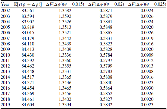
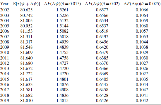
, appear in the last three columns of Tables G1 and G2. We observe that
 $\Delta F(\Delta\psi)$
increases with policyholders’ expected lifespans and decreases with the reinsurance safety loading. Between 2001 and 2019, there is an upward longevity trend, so the expected lifespans of policyholders increase over this period. However, the growth rate of the expected lifespans slows between 2012 and 2019, the growth rate of
 $\Delta F(\Delta\psi)$
also slows in that period, consistent with Remark 4.1 (i) and the results in Djeundje et al. (Reference Djeundje, Haberman, Bajekal and Lu2022). Moreover, relative gains for males are larger than those for females. This difference may reflect that males experience a larger rate of longevity improvement than females.
7. Conclusion
In this paper, we propose a general longevity risk transfer policy for the insurer, aimed at continuously transferring part of benefit payment to the reinsurer to reduce the insurer’s systematic longevity risk exposure. It can be reduced to the traditional longevity risk transfer policies in the recent literature. Compared with the full-transfer policy for the life annuity, the optimal longevity risk transfer policy in this paper leads to lower reinsurance cost and is more acceptable to small- and medium-sized life annuity providers.
Under the expected utility maximization framework with random longevity improvement, we derive that the optimal longevity risk transfer policy takes the form of an excess of age transfer policy. In this way, the insurer is liable for each policyholder’s benefit payment up to a certain age
 $R+T^*$
, and any benefit payment after
 $R+T^*$
is covered by the reinsurer. Therefore, the optimal longevity risk transfer policy exactly offsets the uncertainties in the insurer’s liabilities and reduces the longevity risk exposure. From the reinsurer’s perspective, the optimal excess of age transfer policy reduces the payment burden on the reinsurer and improves the reinsurer’s solvency. We also allow the reinsurer to invest the premium in the financial market and present the condition under which the reinsurer would rationally accept the optimal longevity risk transfer policy proposed by the insurer.
The numerical examples show that the insurer’s relative gains increase when an upward longevity trend exists. In fact, the relative gains
 $\Delta F(\Delta\psi)\gt 0$
when the reinsurance safety loading is relatively low, implying that transferring benefit payment raises the insurer’s terminal wealth when the marginal return exceeds the marginal cost.
We will extend our model to pay-as-you-go pensions. Recent studies such as Alonso-Garcí a et al. (2018) and Morsomme et al. (Reference Morsomme, Alonso-García and Devolder2025) have proposed risk-sharing mechanisms between contributors and retirees to restore the sustainability of pay-as-you-go pension system. The longevity risk transfer policy offers an alternative approach to address the same problem. Given that pay-as-you-go pensions serve as the primary form (first pillar) of life annuity in many countries and are particularly exposed to longevity risk, it is important to apply the longevity risk transfer through reinsurance in this field.
Acknowledgements
This research was supported by the National Natural Science Foundation of China [grant numbers 12371475,12171360, 11871052 and 11771329] and Natural Science Foundation of Tianjin City [grant number 20JCYBJC01160].
Competing interests
We declare that there is no competing interest.
Appendix A. The proof of Proposition 3.1
Proof. From the definition of supremum, there exists a sequence
 $\{g_n(t,b)\}_{n\, \geqslant \, 1}\in\mathcal{G}$
such that
 \begin{equation*} \sup_{g(\cdot,\cdot)\in\mathcal{G}}\mathbb{E}[U(F(g))]=\lim_{n\rightarrow +\infty}\mathbb{E}[U(F(g_n))]\leqslant U(x)\lt +\infty. \end{equation*}
According to Definition 2.1, the sequence
 $\{g_n(t,b)\}_{n\, \geqslant \, 1}$
is uniformly bounded by
 $\sup_{t\in[0,W-R]}\{b(t)\}$
and is uniformly integrable on the closed interval
 $[0,W-R]$
. According to the Dunford–Pettis theorem (Theorem 4.30 in Brézis Reference Brézis2011), there exists a subsequence
 $\{g_{n_k}(t,b) \}_{k\, \geqslant \,1}$
that weakly converges to
 $g^*(t,b)$
in
 $L^1([0,W-R])$
. Then, we obtain that
 $g^*(t,b)\in\mathcal{G}$
, and
 $\lim_{k\rightarrow+\infty}F(g_{n_k})=F(g^*)$
. Applying Fatou’s lemma, we have
 \begin{align*} U(x)-\mathbb{E}[U(F(g^*))]=&\mathbb{E}\left[\lim_{k\rightarrow+\infty}\left(U(x)-U(F(g_{n_k}))\right)\right]\\ \leqslant&\liminf_{k\rightarrow+\infty}\mathbb{E}[U(x)-U(F(g_{n_k}))]\\ =&\mathbb{E}[U(x)]- \sup_{g(\cdot,\cdot)\in\mathcal{G}}\mathbb{E}[U(F(g))], \end{align*}
which implies that
 $\sup_{g(\cdot,\cdot)\in\mathcal{G}}\mathbb{E}[U(F(g))]\leqslant\mathbb{E}[U(F(g^*))]$
. Since
 $\sup_{g(\cdot,\cdot)\in\mathcal{G}}\mathbb{E}[U(F(g))]\, \geqslant \,\mathbb{E}[U(F(g^*))]$
, we obtain
 $\sup_{g(\cdot,\cdot)\in\mathcal{G}}\mathbb{E}[U(F(g))]=\mathbb{E}[U(F(g^*))]$
. Thus,
 $g^*(t,b)$
is the optimal longevity risk transfer policy to Problem (2.5).
Appendix B. The proof of Theroem 3.1
Proof. We first prove that the optimal strategy to problem (2.5) is B
 \begin{align} g^*(t,b)=\left\{ \begin{aligned} &b(t),\quad &H(t;\,g^*)\gt 1+\theta;\\ &0,\quad &H(t;\,g^*)\lt 1+\theta. \end{aligned} \right. \end{align}
For the necessary condition, we assume that
 $g^*(t,b)$
is the optimal strategy to problem (2.5). For any
 $g(t,b)\in \mathcal{G}$
and
 $p\in[0,1]$
, we define the strategy
 $g_p(t,b)=pg^*(t,b)+(1-p)g(t,b)$
, thus
 $g_p(t,b)\in\mathcal{G}$
. The optimality of
 $g^*(t,b)$
implies
 $\frac{\partial \mathbb{E}[U(F(g_p))]}{\partial p}|_{p=1}\, \geqslant \, 0$
, which is equivalent to
 \begin{align} \begin{aligned} 0\leqslant &\mathbb{E}\bigg[U'(F(g^*))\bigg(\frac{1}{n}\sum_{i=1}^n\int_0^{\tau_i(\psi+\Delta\Psi)-R} \mathrm{e}^{-\xi t}[g^*(t,b)-g(t,b)]\mathrm{d} t\\&-(1+\theta)\int_0^\infty \mathrm{e}^{-\xi t}s_R(t+R)[g^*(t,b)-g(t,b)]\mathrm{d} t\bigg)\bigg]\\ =&\frac{1}{n}\sum_{i=1}^n\int_0^\infty\mathbb{E}\left[U'(F(g^*)) \mathrm{e}^{-\xi t}(g^*(t,b)-g(t,b))(\mathbb{I}_{\{t\leqslant\tau_i(\psi+\Delta\Psi)-R\}}-(1+\theta)s_R(t+R))\right]\mathrm{d} t\\ =&\int_0^\infty \mathrm{e}^{-\xi t}(g^*(t,b)-g(t,b))s_R(t+R)\mathbb{E}[U'(F(g^*))]\left(H(t;\,g^*)-(1+\theta)\right)\mathrm{d} t, \end{aligned} \end{align}
where the last equality follows from the fact that
 $\{\tau_i(\psi+\Delta\Psi)\}_{i=1,\ldots,n}$
are conditionally independent and identically distributed. If Equation (3.1) is not satisfied, there exists a nonempty set
 $M\subseteq [0,W-R)$
such that either
 $g^*(t,b)\lt b(t)$
with
 $H(t;\,g^*)\gt 1+\theta$
for all
 $t\in M$
or
 $g^*(t,b)\gt 0$
with
 $H(t;\,g^*)\lt 1+\theta$
for all
 $t\in M$
. In the first case, let
 $g(t,b)=b(t)$
for any
 $t\in M$
and
 $g(t,b)=g^*(t,b)$
for any
 $t\in M^c$
. Therefore, Equation (B.2) turns into
 \begin{align} \int_{M} \mathrm{e}^{-\xi t}(g^*(t,b)-b(t))s_R(t+R)\mathbb{E}[U'(F(g^*))](H(t;\,g^*)-(1+\theta))\mathrm{d} t\lt 0, \end{align}
where the inequality follows from the fact that
 $U'(\!\cdot\!)\gt 0$
,
 $s_R(t+R)\gt 0$
,
 $H(t;\,g^*)-(1+\theta)\gt 0$
and
 $g^*(t,b)-b(t)\lt 0$
for any
 $t\in M$
. This contradicts Equation (B.2). In the second case, let
 $g(t,b)=0$
for any
 $t\in M$
and
 $g(t,b)=g^*(t,b)$
for any
 $t\in M^c$
. We derive the similar contradiction as shown in Equation (B.3) by the fact
 $H(t;\,g^*)-(1+\theta)\lt 0$
and
 $g^*(t,b)\gt 0$
for any
 $t\in M$
.
Hereafter, we focus on the sufficiency of Equation (3.1). If Equation (3.1) is satisfied, based on the concavity of the utility function
 $U(\!\cdot\!)$
, for any
 $g(t,b)\in \mathcal{G}$
, we have
 \begin{align*} &\mathbb{E}[U(F(g^*))]-\mathbb{E}[U(F(g))]\\ \, \geqslant \, &\mathbb{E}\bigg[U'(F(g^*))\bigg(\frac{1}{n}\sum_{i=1}^n\int_0^{\tau_i(\psi+\Delta\Psi)-R} \mathrm{e}^{-\xi t}[g^*(t,b)-g(t,b)]\mathrm{d} t\\ &-(1+\theta)\int_0^\infty \mathrm{e}^{-\xi t}s_R(t+R)[g^*(t,b)-g(t,b)]\mathrm{d} t\bigg)\bigg]\\ =&\int_0^\infty \mathrm{e}^{-\xi t}(g^*(t,b)-g(t,b))s_R(t+R)\mathbb{E}[U'(F(g^*))](H(t;\,g^*)-(1+\theta))\mathrm{d} t\\ \, \geqslant \,& 0. \end{align*}
Therefore,
 $g^*(t,b)$
as defined in Equation (B.1) is the optimal solution to problem (2.5).
Furthermore, the integral
 $\int_t^{t+\Delta t}g(\nu,b)\mathrm{d} \nu$
denotes the transfer amount over period
 $[t,t+\Delta t]$
, and g(t,b) specifies a transfer rate at time t. In later discussion, we can prove that
 $H(t;\,g^*)$
has at most one intersection with
 $1+\theta$
, then the cumulative transfer
 $\int_t^{t+\Delta}g^*(\nu,b)\mathrm{d} \nu$
remains unchanged, regardless of whether
 $g^*(t,b)=0$
or
 $g^*(t,b)=b(t)$
at this intersection point. Therefore, the optimal longevity risk transfer policy
 $g^*(t,b)$
satisfies Equation (3.1) almost everywhere, and its value on the set
 $\{t\in[0,W-R]|H(t;\,g^*)=1+\theta\}$
, which has zero Lebesgue measure, does not affect the cumulative transfer. To match the excess of age transfer policy in Equation (2.2), we set
 \begin{align*} g^*(t,b)=\left\{ \begin{aligned} &b(t),\quad &H(t;\,g^*)\, \geqslant \,1+\theta;\\ &0,\quad &H(t;\,g^*)\lt 1+\theta. \end{aligned} \right. \end{align*}
Appendix C. The proof of Corollary 3.1 and Lemma 3.1
C.1. The proof of Corollary 3.1
Proof. For any
 $t\in[0,W-R]$
, we have
 \begin{align} \begin{aligned} H(t;\,g^*)-(1+\theta)=&\frac{\mathbb{E}\left[U'(F(g))\mathbb{I}_{\{\tau_i(\psi+\Delta\Psi)\, \geqslant \, t+R\}}\right]}{\mathbb{E}\left[U'(F(g))\right]s_R(t+R)}-(1+\theta)\\ \leqslant&\frac{1}{s_R(t+R)}-(1+\theta), \end{aligned} \end{align}
so if
 $t\in[0,T_{\theta}]$
, we have
 $H(t;\,g^*)-(1+\theta)\leqslant 0$
, which implies that
 $g^*(t,b)=0$
.
C.2. The proof of Lemma 3.1
Proof. (i) We find that
 $\lim_{\varepsilon\rightarrow+\infty}H(t+\varepsilon ; \, g)=H(t; \, g)$
, which implies that the function
 $H(t; \, g)$
is a continuous function with respect to t. Since the denominator of
 $H(t; \, g)$
is independent of t, the monotonicity of
 $H(t; \, g)$
depends only on the monotonicity of its numerator. We first introduce the following notation
 \begin{align*} \hat{F}(s_i; \,g)=\int_0^{s_i-R} \mathrm{e}^{-\xi t}(b(t)-g(t,b))\mathrm{d} t+(1+\theta)\int_0^\infty \mathrm{e}^{-\xi t}s_R(t+R) g(t,b)\mathrm{d} t, \end{align*}
 \begin{align*} \hat{H}(t)&=\mathbb{E}\left[U'\left(x-\frac{1}{n}\sum_{j=1}^n\hat{F}(\tau_j(\psi+\Delta\Psi); \,g)\right)\bigg|\tau_i(\psi+\Delta\Psi)\, \geqslant \, t+R,\Delta\Psi=\Delta\psi\right]\\ &=\frac{\int_R^W\ldots\int_{t+R}^W\ldots\int_R^WU'(x-\frac{1}{n}\sum_{j=1}^n\hat{F}(v_j; \,g^*))f(v_1,\ldots,v_n|\Delta\Psi=\Delta\psi)\mathrm{d} v_1\ldots\mathrm{d} v_i\ldots\mathrm{d} v_n}{S_R(t+R;\,\psi+\Delta\psi)}, \end{align*}
where
 $f(v_1,\ldots,v_n|\Delta\Psi=\Delta\psi)$
is the conditional joint distribution for
 $\{\tau_i(\psi+\Delta\psi)\}_{i=1,\ldots,n}$
. For any given
 $\Delta\Psi=\Delta\psi$
, since
 $\{\tau_i(\psi+\Delta\psi)\}_{i=1,\ldots,n}$
are independent and identically distributed, we have
 $f(v_1,\ldots,v_n|\psi+\Delta\psi)=(f_{\tau|\Delta\Psi}(v_j|\psi+\Delta\psi))^n$
, where
 $f_{\tau|\Delta\Psi}(v_j|\psi+\Delta\psi)$
represents the conditional marginal distribution. Then, we have
 \begin{align*} \hat{H}'(t)&=\frac{f_{\tau|\Delta\Psi}(t+R|\psi+\Delta\psi)}{S_R(t+R;\,\psi+\Delta\psi)}\bigg(-\mathbb{E}\left[U'\left(x-\frac{1}{n}\sum_{j=1}^n\hat{F}(\tau_j(\psi+\Delta\Psi); \,g)\right) \bigg|\tau_i(\psi+\Delta\Psi)=t+R,\Delta\Psi \right. \\&=\Delta\psi \bigg. \bigg ] +\hat{H}(t)\bigg) \gt 0, \end{align*}
where the inequality follows from the fact that
 $\hat{F}(v_i; \,g) \lt \hat{F}(t+R; \,g)$
for any
 $v_i\in[t+R,W]$
and
 $U''(\!\cdot\!)\lt 0$
. This implies that
 $H(t; \, g)$
is a strictly increasing function.
(ii) By calculating the limit of
 $\hat{H}(t)$
, we obtain
 \begin{align*} \lim_{t\rightarrow W-R}\hat{H}(t)\,=\,&\lim_{t\rightarrow W-R}\frac{\int_R^W\ldots\int_{t+R}^W\ldots\int_R^WU' \big(x-\frac{1}{n}\sum_{j=1}^n\hat{F}(v_j; \,g^*) \big)f(v_1,{\ldots},v_n|\Delta\Psi=\Delta\psi)\mathrm{d} v_1{\ldots}\mathrm{d} v_i{\ldots}\mathrm{d} v_n}{S_R(t+R;\,\psi+\Delta\psi)}\\ \,=\, &\mathbb{E} \bigg[U' \bigg(x-\frac{1}{n}\hat{F}(W; \,g)-\frac{1}{n}\sum_{j\neq i}\hat{F}(\tau_j(\psi+\Delta\Psi)) \bigg) |\Delta\Psi=\Delta\psi \bigg]. \end{align*}
Obviously, we have
 $\lim_{t\rightarrow W-R}\frac{\mathbb{E}[\hat{H}(t)]}{\mathbb{E}\left[U'(x-\frac{1}{n}\sum_{i=1}^n\hat{F}(\tau_i; \,g))\right]}\gt 1$
and
 $H(0;\,g)=1$
. Since
 $H(t; \, g)$
is an increasing function with respect to t, we derive
 $H(t; \, g)$
is bounded.
Appendix D. The proof of Theorem 3.2
Proof. According to Lemma 3.1, the optimal longevity risk transfer policy defined in Theorem 3.1 can be simplified into an excess of age transfer policy. We aim to show that when substituting Equation (3.3) into Theorem 3.1, the inequality
 $H(t;\,g_{T^*})\lt 1+\theta$
holds for any
 $t\in[0,T^*]$
, and
 $H(t;\,g_{T^*})\gt 1+\theta$
holds for any
 $t\gt T^*$
.
By convention, we set
 $\inf\emptyset=\infty$
. If
 $T^*\leqslant W-R$
, then for any
 $t\in[T_\theta,T^*)$
, we obtain
 $\mathcal{H}(t)\lt 1+\theta$
, and we have
 \begin{align} \begin{aligned} H(t;\,g_{T^*})=&\frac{\mathbb{E}\left[U'\left(x-\frac{1}{n}\sum_{j=1}^n\hat{F}(\tau_j(\psi+\Delta\Psi); \, T^*)\right)|\tau_i(\psi+\Delta\Psi)\, \geqslant \, t+R\right]}{\mathbb{E}\left[U'\left(x-\frac{1}{n}\sum_{j=1}^n\hat{F}(\tau_j(\psi+\Delta\Psi) ; \,{T^*})\right)\right]}\\ =&\lim_{s\uparrow T^*,s\gt t}\frac{\mathbb{E}\left[U'\left(x-\frac{1}{n}\sum_{j=1}^n\hat{F}(\tau_j(\psi+\Delta\Psi);\,s)\right)|\tau_i(\psi+\Delta\Psi)\, \geqslant \, t+R\right]}{\mathbb{E}\left[U'\left(x-\frac{1}{n}\sum_{j=1}^n\hat{F}(\tau_j(\psi+\Delta\Psi);\,s)\right)\right]}\\ \leqslant&\lim_{s\uparrow T^*,s\gt t}\frac{\mathbb{E}\left[U'\left(x-\frac{1}{n}\sum_{j=1}^n\hat{F}(\tau_j(\psi+\Delta\Psi);\,s)\right)|\tau_i(\psi+\Delta\Psi)\, \geqslant \, s+R\right]}{\mathbb{E}\left[U'\left(x-\frac{1}{n}\sum_{j=1}^n\hat{F}(\tau_j(\psi+\Delta\Psi);\,s)\right)\right]}\\ =&\lim_{s\uparrow T^*,s\gt t}\mathcal{H}(s)\\ \lt &1+\theta, \end{aligned} \end{align}
where the first inequality follows from Lemma 3.1. Besides, since
 $H(t; \, g)$
is an increasing function with respect to t, for any
 $t\, \geqslant \, T^*$
, we obtain that
 \begin{equation} H(t;\,g_{T^*})\gt H(T^*; \,g_{T^*})=\mathcal{H}(T^*)\, \geqslant \,1+\theta. \end{equation}
From Equations (D.1) and (D.2) together with Theorem 3.1, the transfer policy defined in Equation (3.3) is the optimal policy to Equation (2.5).
If
 $T^*\gt W-R$
, we have
 $\inf\{T\in[T_\theta,W-R] \, : \, \mathcal{H}(T)\, \geqslant \,1+\theta\}=\emptyset$
, and
 $\mathcal{H}(t)\lt 1+\theta$
for all
 $t\in[T_\theta,W-R]$
. By substituting
 $T^*$
into Equation (3.3), for any
 $t\in[T_\theta,W-R]$
, we derive that
 \begin{align*} 1+\theta\gt &\lim_{s\uparrow W-R}\mathcal{H}(s)\\=&\lim_{s\uparrow W-R}\frac{\mathbb{E}\left[U'\left(x-\frac{1}{n}\sum_{j=1}^n\hat{F}(\tau_j(\psi+\Delta\Psi);\,s)\right)|\tau_i(\psi+\Delta\Psi)\, \geqslant \, s+R\right]}{\mathbb{E}\left[U'\left(x-\frac{1}{n}\sum_{j=1}^n\hat{F}(\tau_j(\psi+\Delta\Psi);\,s)\right)\right]}\\ =&\frac{\lim_{s\uparrow W-R}\mathbb{E}\left[U'\left(x-\frac{1}{n}\sum_{j=1}^n\int_0^{\tau_j(\psi+\Delta\Psi)-R}\mathrm{e}^{-\xi t} b(t)\mathrm{d} t\right)|\tau_i(\psi+\Delta\Psi)\, \geqslant \, s+R\right]}{\mathbb{E}\left[U'\left(x-\frac{1}{n}\sum_{j=1}^n\int_0^{\tau_j(\psi+\Delta\Psi)-R}\mathrm{e}^{-\xi t} b(t)\mathrm{d} t\right)\right]}\\ \, \geqslant \,& H(t;\,g_{T^*}). \end{align*}
Therefore, it follows that the strategy
 $g_{T^*}(t,b)$
is the optimal longevity risk transfer policy, which means that
 $g^*(t,b)=g_{T^*}(t,b)$
. Similar to the discussion in Theorem 3.1, we set that the policy
 $g^*(t,b)=b(t)$
when
 $t=T^*$
. Then, the optimal longevity risk transfer policy is given by
 $g^*(t,b)=b(t)\mathbb{I}_{\{t\, \geqslant \, T^*\}}$
.
Appendix E. The proof of Proposition 3.2
Proof. If either
 $g^{(1)}(t,b)$
or
 $g^{(2)}(t,b)$
is the optimal solutions to Problem (2.5), we have
 \begin{equation*} \mathbb{E}[U(F(g^{(1)}))]=\mathbb{E}[U(F(g^{(2)}))]=M. \end{equation*}
For any
 $p\in(0,1)$
, let
 $\tilde{g}(t,b)=pg^{(1)}(t,b)+(1-p)g^{(2)}(t,b)$
. For convenience, we denote that
 $G(t,b)=g^{(1)}(t,b)-g^{(2)}(t,b)$
. We verify that
 $\tilde{g}(t,b)\in\mathcal{G}$
, and
 $\mathbb{E}[U(F(\tilde{g}))]\leqslant M$
. By the concavity of
 $U(\!\cdot\!)$
, it follows that
 \begin{equation} \mathbb{E}[U(F(\tilde{g}))]\, \geqslant \, p\mathbb{E}[U(F(g^{(1)}))]+(1-p)\mathbb{E}[U(F(g^{(2)}))]=M. \end{equation}
Therefore, the equality in Equation (E.1) is obtained. Furthermore, Equation (E.1) implies that
 $F(g^{(1)})\buildrel \mathrm{a.s.} \over = F(g^{(2)})$
. It leads to
 \begin{equation*} \sum_{i=1}^n\int_0^{\tau_i(\psi+\Delta\Psi)-R} \mathrm{e}^{-\xi t}G(t,b)\mathrm{d} t\buildrel \mathrm{a.s.} \over =(1+\theta)n\int_0^\infty \mathrm{e}^{-\xi t}s_R(t+R) G(t,b)\mathrm{d} t. \end{equation*}
If
 $\theta\gt 0$
, we obtain
 $\mathbb{E}[\int_0^{\tau_i(\psi+\Delta\Psi)-R} \mathrm{e}^{-\xi t}G(t,b)\mathrm{d} t]=0$
. It means that the optimal longevity risk transfer policy is unique in the sense that
 \begin{equation*} \int_0^{\tau_i(\psi+\Delta\Psi)-R}\mathrm{e}^{-\xi t}g^{(1)}(t,b)\mathrm{d} t\buildrel \mathrm{a.s.} \over =\int_0^{\tau_i(\psi+\Delta\Psi)-R}\mathrm{e}^{-\xi t}g^{(2)}(t,b)\mathrm{d} t,\quad \forall i\in\{1,\ldots,n\}. \end{equation*}
If
 $\theta=0$
, we have
 \begin{equation*} \sum_{i=1}^n\int_0^{\tau_i(\psi+\Delta\Psi)-R} \mathrm{e}^{-\xi t}G(t,b)\mathrm{d} t\buildrel \mathrm{a.s.} \over = n\int_0^\infty \mathrm{e}^{-\xi t}s_R(t+R) G(t,b)\mathrm{d} t. \end{equation*}
It implies that
 $\mathbb{P}((\tau_1(\psi+\Delta\Psi)),\ldots,\tau_n(\psi+\Delta\Psi))\in\mathcal{A})=1$
, where
 $\mathcal{A}$
is given by
 \begin{equation*} \mathcal{A}=\left\{(t_1,\ldots,t_n)\in[R,W]^n\, : \,\sum_{i=1}^n\int_0^{t_i-R} \mathrm{e}^{-\xi t}G(t,b)\mathrm{d} t=n\int_0^\infty \mathrm{e}^{-\xi t}s_R(t+R) G(t,b)\mathrm{d} t\right\}. \end{equation*}
If
 $(t_1,\ldots,t_n)=(R,\ldots,R)\in\mathcal{A}$
, we derive
 $\int_0^\infty \mathrm{e}^{-\xi t}s_R(t+R) G(t,b)\mathrm{d} t=0$
, which implies that
 $\int_0^{\tau_i(\psi+\Delta\Psi)-R}\mathrm{e}^{-\xi t}g^{(1)}(t,b)\mathrm{d} t\buildrel \mathrm{a.s.} \over =\int_0^{\tau_i(\psi+\Delta\Psi)-R}\mathrm{e}^{-\xi t}g^{(2)}(t,b)\mathrm{d} t$
holds for all
 $i\in\{1,\ldots,n\}$
.
If
 $(t_1,\ldots,t_n)=(R,\ldots,R)\notin\mathcal{A}$
, there exists a index separation
 $\{i_k\}_{k\, \geqslant \,1}\cup\{j_m\}_{m\, \geqslant \,1}=\{1,2,\ldots,n\}$
, such that
 $\{t_{j_m}=l_{j_m}\}_{m\, \geqslant \,1}\cup\{t_{i_k}=R\}_{k\, \geqslant \,1}\in\mathcal{A}$
holds for some constants
 $l_{j_m}\in(R,W]$
. Since the support of
 $\tau(\psi+\Delta\Psi)$
is [R,W], we have
 \begin{equation} \mathbb{P}((\tau_1(\psi+\Delta\Psi)),\ldots,\tau_n(\psi+\Delta\Psi))\in B(\boldsymbol{\nu},\varepsilon))\gt 0,\quad \forall \boldsymbol{\nu}\in[R,W]^n, \forall\varepsilon\gt 0, \end{equation}
where
 $B(\boldsymbol{\nu},\varepsilon)=\{\mathbf{c}\in[R,W]^n \, : \,||\boldsymbol{c}-\boldsymbol{\nu}||\leqslant\varepsilon\}$
is the n-dimensional open neighborhood of
 $\boldsymbol{\nu}$
. For any fixed
 $l\, \geqslant \,1$
, and take
 $\varepsilon=\frac{1}{l}$
, we obtain
 \begin{equation*} \begin{aligned} { \mathbb{P}}(({\tau_1}(\psi+{\Delta}\Psi)),{\ldots},{\tau_n}(\psi+\Delta\Psi))\in\mathcal{A}{\cap} B(\boldsymbol{R},\varepsilon))=\mathbb{P}(({\tau_1}(\psi+\Delta\Psi)),{\ldots},{\tau_n}(\psi+\Delta\Psi)){\in} B(\boldsymbol{R},{\varepsilon}))\gt {0}. \end{aligned} \end{equation*}
Therefore, there exists a sequence
 $\{t^{(l)}_{j_m}\}_{l\, \geqslant \,1}$
such that
 $\lim_{l\rightarrow+\infty}t^{(l)}_{j_m}=R$
and
 $\{t_{j_m}=t^{(l)}_{j_m}\}_{m\, \geqslant \,1}\cup\{t_{i_k}=R\}_{k\, \geqslant \,1}\in\mathcal{A}$
. We have
 \begin{equation} n\int_0^\infty \mathrm{e}^{-\xi t}s_R(t+R) G(t,b)\mathrm{d} t=\lim_{l\rightarrow+\infty}\sum_{j\in\{j_m\}_{m\, \geqslant \,1}}\int_0^{t^{(l)}_{j}-R} \mathrm{e}^{-\xi t}G(t,b)\mathrm{d} t=0. \end{equation}
Since the optimal longevity risk transfer policy satisfies the excess of age transfer policy, we obtain that
 \begin{equation*} 0=\int_0^\infty \mathrm{e}^{-\xi t}s_R(t+R) b(t)(\mathbb{I}_{\{t\, \geqslant \, T^{(1)}\}}-\mathbb{I}_{\{t\, \geqslant \, T^{(2)}\}})\mathrm{d} t, \end{equation*}
which leads to
 $T^{(1)}=T^{(2)}$
.
Appendix F. The proof of Proposition 5.1
Proof. (i) We observe that
 $\mathbb{E}[-W_R(r;\,\psi+\Delta\Psi)]+\delta\varrho(-W_R(r;\,\psi+\Delta\Psi)-\mathbb{E}[-W_R(r;\,\psi+\Delta\Psi)])$
is a decreasing function with respect to r. Besides, we obtain F
 \begin{equation} \lim_{r\rightarrow +\infty}\mathbb{E}[-W_R(r;\,\psi+\Delta\Psi)]+\delta\varrho(-W_R(r;\,\psi+\Delta\Psi)-\mathbb{E}[-W_R(r;\,\psi+\Delta\Psi)])=-\infty. \end{equation}
This implies that there exists
 $\bar{r}$
as defined in Equation (5.3), thus Equation (5.2) holds for any
 $r\, \geqslant \,\bar{r}$
.
(ii) According to the property of law-invariant coherent risk measure
 $\rho(\!\cdot\!)$
, we have
 \begin{align} {J_R}{(r;\,\psi_1+\Delta\psi)}=&(1-\delta)n\int_0^{\infty }\mathrm{e}^{-\xi t}S_R(t+R;\,\psi+\Delta\psi)b(t)\mathbb{I}_{\{t\gt T^*\}}\mathrm{d} t+\delta\rho\left(\sum_{i=1}^n\int_0^{\tau_i(\psi+\Delta\psi)-R} \right. \nonumber \\&e^{-\xi t}b(t)\mathbb{I}_{\{t\gt T^*\}}{\mathrm{d}t} \left. \right) -(1+\theta) \mathrm{e}^{(r-\xi)T^*}n\int_0^{\infty} {\mathrm{e}}^{-\xi t}s_R(t+R)b(t){\mathbb{I}}_{\{t\gt T^*\}}\mathrm{d} t. \end{align}
Besides, by Kusuoka’s theorem (Theorem 4 in Kusuoka Reference Kusuoka2001), there exists a set of probability measures
 $\mathcal{M}$
on [0,1] such that the second term in Equation (F.2) can be rewritten as
 \begin{equation*} \rho\left(\sum_{i=1}^n\int_0^{\tau_i(\psi+\Delta\psi)-R}e^{-\xi t}b(t)\mathbb{I}_{\{t\gt T^*\}}\mathrm{d} t\right)=\sup_{\mu\in\mathcal{M}}\int_0^1\mathrm{CVaR}_{\alpha}\left(\sum_{i=1}^n\int_0^{\tau_i(\psi+\Delta\psi)-R}e^{-\xi t}b(t)\mathbb{I}_{\{t\gt T^*\}}\mathrm{d} t\right)\mathrm{d}\mu(\alpha). \end{equation*}
Since
 $S_R(t;\,\psi)$
is increasing in
 $\psi$
, for any
 $\Delta\psi\leqslant\Delta\psi'$
, it follows that
 \begin{equation*} \int_0^{\tau_i(\psi+\Delta\psi)-R}e^{-\xi t}b(t)\mathbb{I}_{\{t\gt T^*\}}\mathrm{d} t\leqslant_{\mathrm{FSD}}\int_0^{\tau_i(\psi+\Delta\psi')-R}e^{-\xi t}b(t)\mathbb{I}_{\{t\gt T^*\}}\mathrm{d} t, \end{equation*}
where
 $\leqslant_{\mathrm{FSD}}$
represents the first-order stochastic dominance. Therefore, we derive
 \begin{equation*} \sum_{i=1}^n\int_0^{\tau_i(\psi+\Delta\psi)-R}e^{-\xi t}b(t)\mathbb{I}_{\{t\gt T^*\}}\mathrm{d} t\leqslant_{\mathrm{FSD}} \sum_{i=1}^n\int_0^{\tau_i(\psi+\Delta\psi')-R}e^{-\xi t}b(t)\mathbb{I}_{\{t\gt T^*\}}\mathrm{d} t. \end{equation*}
Since the risk measure
 $\mathrm{CVaR}_{\alpha}(\!\cdot\!)$
preserves first-order stochastic dominance, we have
 \begin{equation} \rho\left(\sum_{i=1}^n \int_0^{\tau_i(\psi+\Delta\psi)-R}e^{-\xi t}b(t)\mathbb{I}_{\{t\gt T^*\}}\mathrm{d} t\right)\leqslant \rho\left(\sum_{i=1}^n\int_0^{\tau_i(\psi+\Delta\psi')-R}e^{-\xi t}b(t)\mathbb{I}_{\{t\gt T^*\}}\mathrm{d} t\right), \end{equation}
which means that
 $\rho\left(\sum_{i=1}^n\int_0^{\tau_i(\psi+\Delta\psi)-R}e^{-\xi t}b(t)\mathbb{I}_{\{t\gt T^*\}}\mathrm{d} t\right)$
is increasing in
 $\Delta\psi$
. Therefore, it follows that
 $J_R(r;\,\psi+\Delta\psi)$
is increasing in
 $\Delta\psi$
.
Appendix G. Numerical example for annual relative gains
${\Delta} \textit{F}(\Delta{\psi})$

Numerical results for female.

Table G1 Long description
A table with 19 rows and 5 columns. The columns are labeled Year, E[τ(ψ + Δψ)], ΔF(Δψ)(θ = 0.015), ΔF(Δψ)(θ = 0.02), and ΔF(Δψ)(θ = 0.025). The table presents data for each year from 2002 to 2019. Each row lists the year, followed by four numerical values corresponding to the columns. Notable trends include a general increase in the values of E[τ(ψ + Δψ)] over the years, indicating an upward longevity trend. The values of ΔF(Δψ) for different θ values also show variations across the years, with a general pattern of increasing and then stabilizing.
Numerical results for male.

Table G2 Long description
A table with 19 rows and 5 columns. The columns are labeled Year, E[τ(ψ + Δψ)], ΔF(Δψ)(θ = 0.015), ΔF(Δψ)(θ = 0.02), and ΔF(Δψ)(θ = 0.025). The table presents data on the expected lifespans and relative gains for males in the United States from 2002 to 2019. Row 1: Year, 2002; E[τ(ψ + Δψ)], 80.625; ΔF(Δψ)(θ = 0.015), 1.5261; ΔF(Δψ)(θ = 0.02), 0.6577; ΔF(Δψ)(θ = 0.025), 0.1066. Row 2: Year, 2003; E[τ(ψ + Δψ)], 80.742; ΔF(Δψ)(θ = 0.015), 1.5226; ΔF(Δψ)(θ = 0.02), 0.6566; ΔF(Δψ)(θ = 0.025), 0.1064. Row 3: Year, 2004; E[τ(ψ + Δψ)], 81.005; ΔF(Δψ)(θ = 0.015), 1.5132; ΔF(Δψ)(θ = 0.02), 0.6534; ΔF(Δψ)(θ = 0.025), 0.1059. Row 4: Year, 2005; E[τ(ψ + Δψ)], 80.952; ΔF(Δψ)(θ = 0.015), 1.5144; ΔF(Δψ)(θ = 0.02), 0.6537; ΔF(Δψ)(θ = 0.025), 0.1060. Row 5: Year, 2006; E[τ(ψ + Δψ)], 81.153; ΔF(Δψ)(θ = 0.015), 1.5082; ΔF(Δψ)(θ = 0.02), 0.6519; ΔF(Δψ)(θ = 0.025), 0.1057. Row 6: Year, 2007; E[τ(ψ + Δψ)], 81.311; ΔF(Δψ)(θ = 0.015), 1.5018; ΔF(Δψ)(θ = 0.02), 0.6497; ΔF(Δψ)(θ = 0.025), 0.1053. Row 7: Year, 2008; E[τ(ψ + Δψ)], 81.317; ΔF(Δψ)(θ = 0.015), 1.4939; ΔF(Δψ)(θ = 0.02), 0.6456; ΔF(Δψ)(θ = 0.025), 0.1044. Row 8: Year, 2009; E[τ(ψ + Δψ)], 81.548; ΔF(Δψ)(θ = 0.015), 1.4839; ΔF(Δψ)(θ = 0.02), 0.6420; ΔF(Δψ)(θ = 0.025), 0.1038. Row 9: Year, 2010; E[τ(ψ + Δψ)], 81.609; ΔF(Δψ)(θ = 0.015), 1.4755; ΔF(Δψ)(θ = 0.02), 0.6379; ΔF(Δψ)(θ = 0.025), 0.1029. Row 10: Year, 2011; E[τ(ψ + Δψ)], 81.640; ΔF(Δψ)(θ = 0.015), 1.4758; ΔF(Δψ)(θ = 0.02), 0.6385; ΔF(Δψ)(θ = 0.025), 0.1030. Row 11: Year, 2012; E[τ(ψ + Δψ)], 81.680; ΔF(Δψ)(θ = 0.015), 1.4727; ΔF(Δψ)(θ = 0.02), 0.6370; ΔF(Δψ)(θ = 0.025), 0.1027. Row 12: Year, 2013; E[τ(ψ + Δψ)], 81.672; ΔF(Δψ)(θ = 0.015), 1.4720; ΔF(Δψ)(θ = 0.02), 0.6366; ΔF(Δψ)(θ = 0.025), 0.1026. Row 13: Year, 2014; E[τ(ψ + Δψ)], 81.722; ΔF(Δψ)(θ = 0.015), 1.4720; ΔF(Δψ)(θ = 0.02), 0.6369; ΔF(Δψ)(θ = 0.025), 0.1027. Row 14: Year, 2015; E[τ(ψ + Δψ)], 81.617; ΔF(Δψ)(θ = 0.015), 1.4801; ΔF(Δψ)(θ = 0.02), 0.6405; ΔF(Δψ)(θ = 0.025), 0.1035. Row 15: Year, 2016; E[τ(ψ + Δψ)], 81.633; ΔF(Δψ)(θ = 0.015), 1.4876; ΔF(Δψ)(θ = 0.02), 0.6445; ΔF(Δψ)(θ = 0.025), 0.1044. Row 16: Year, 2017; E[τ(ψ + Δψ)], 81.581; ΔF(Δψ)(θ = 0.015), 1.4908; ΔF(Δψ)(θ = 0.02), 0.6458; ΔF(Δψ)(θ = 0.025), 0.1047. Row 17: Year, 2018; E[τ(ψ + Δψ)], 81.682; ΔF(Δψ)(θ = 0.015), 1.4836; ΔF(Δψ)(θ = 0.02), 0.6428; ΔF(Δψ)(θ = 0.025), 0.1041. Row 18: Year, 2019; E[τ(ψ + Δψ)], 81.810; ΔF(Δψ)(θ = 0.015), 1.4815; ΔF(Δψ)(θ = 0.02), 0.6426; ΔF(Δψ)(θ = 0.025), 0.1042.

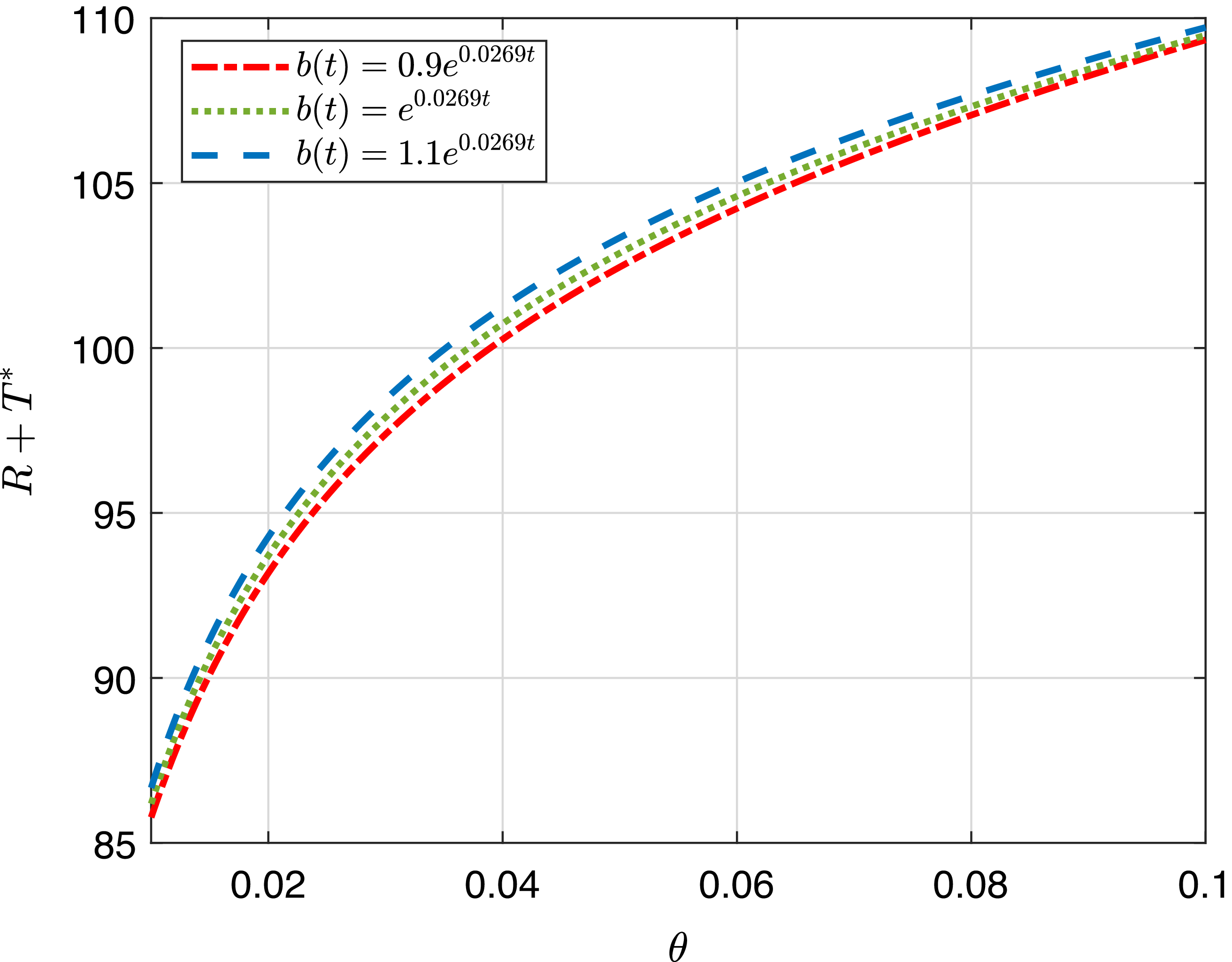
 θ
 T∗
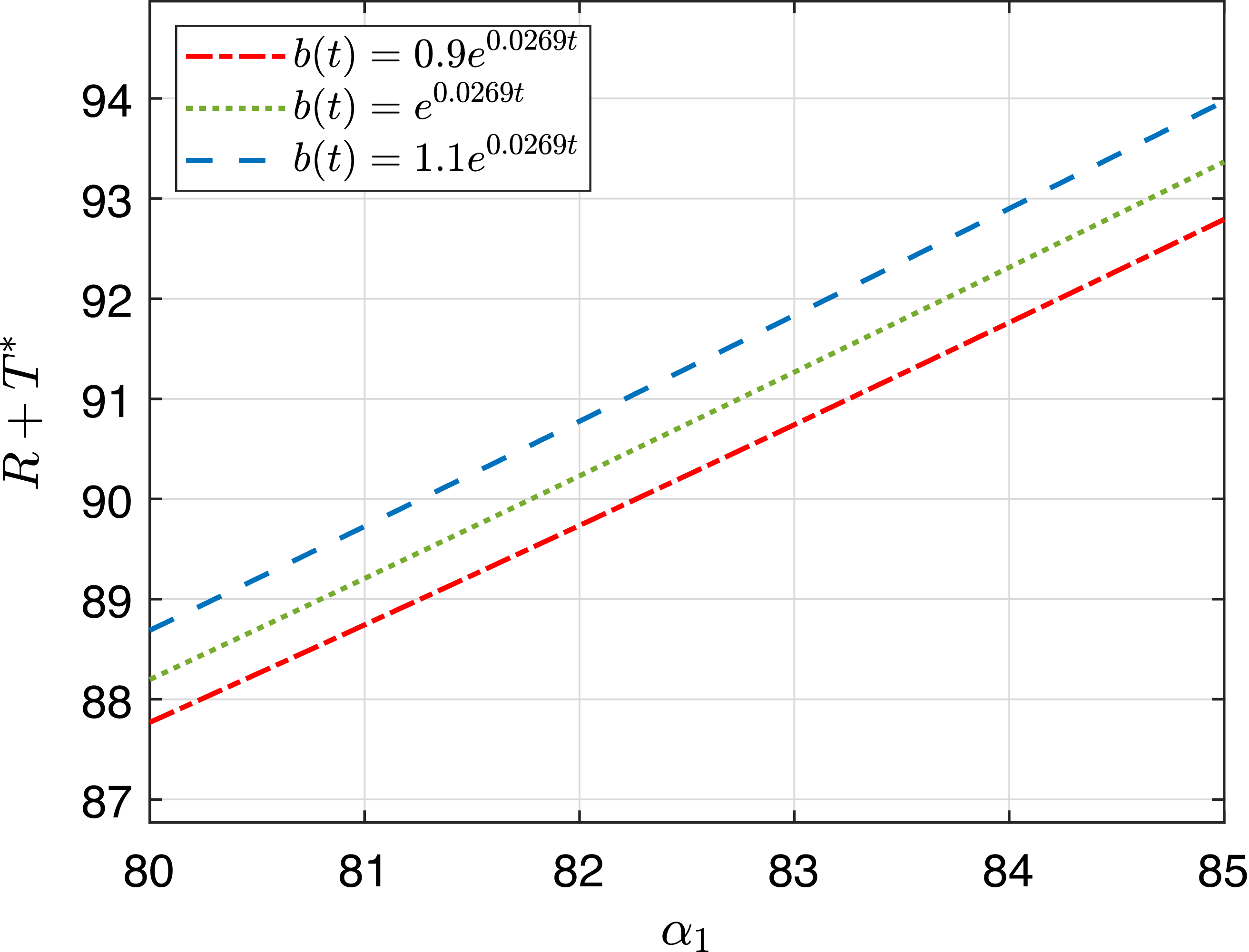
 ψ
 T∗
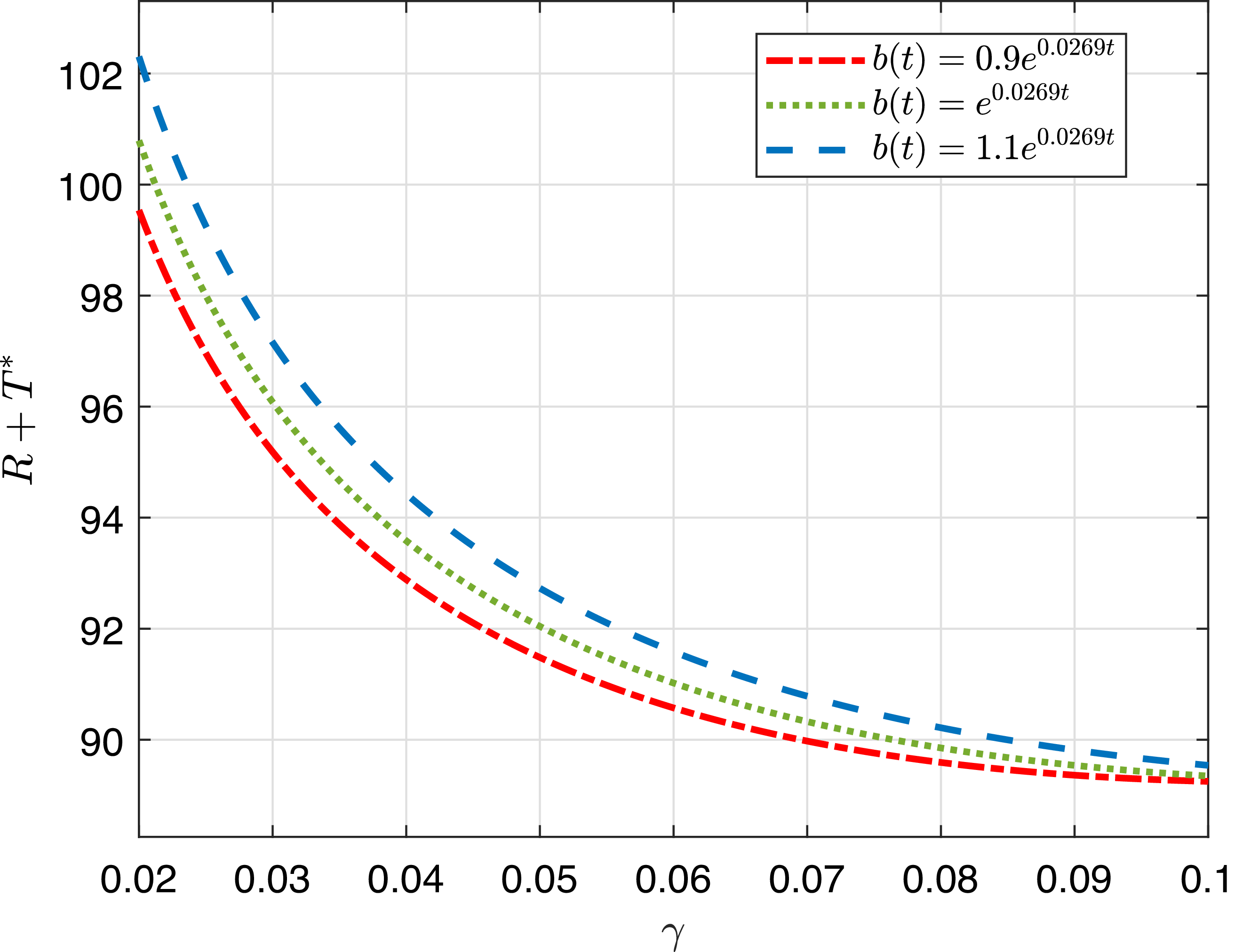
 γ
 R+T∗
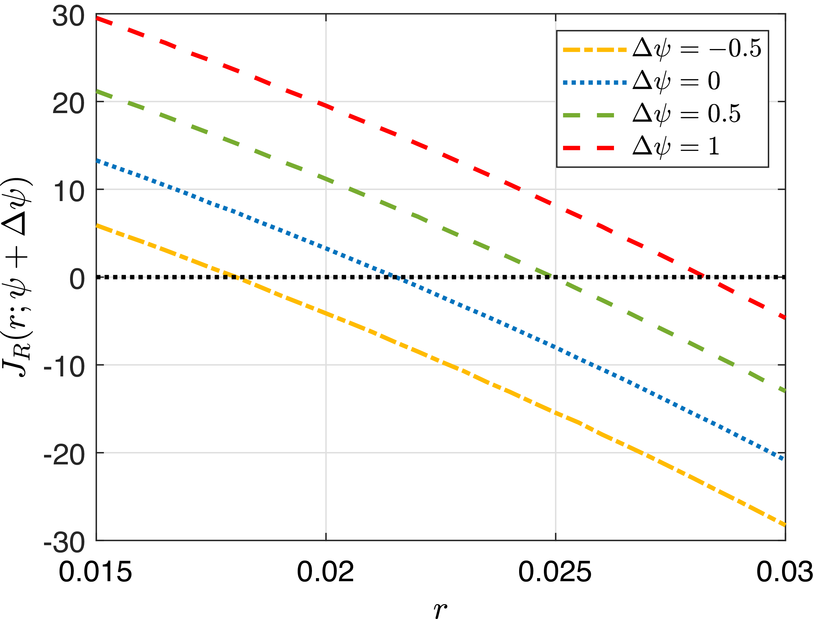
 Δψ
 R+T∗