1. Introduction
The dynamics of elastic particles, both sedimenting and entrained by an ambient flow, attracts a lot of attention owing to the importance of many-particle systems of flexible fibres, vesicles or capsules for industry, biology, medicine and nano-technology, as emphasized e.g. by Dreyfus et al. (Reference Dreyfus, Baudry, Roper, Fermigier, Stone and Bibette2005), Drescher et al. (Reference Drescher, Leptos, Tuval, Ishikawa, Pedley and Goldstein2009), Vlahovska, Podgorski & Misbah (Reference Vlahovska, Podgorski and Misbah2009) and Kantsler & Goldstein (Reference Kantsler and Goldstein2012). Deformation and the existence of constraint forces lead to very complex dynamics even in the case of isolated particles, and to significant modifications of hydrodynamic interactions between such objects. For example, there exist different modes of the dynamics, analysed e.g. by Young & Shelley (Reference Young and Shelley2007), or migration and accumulation of isolated flexible particles in ambient flows, as shown e.g. by Farutin & Misbah (Reference Farutin and Misbah2013) and Słowicka, Wajnryb & Ekiel-Jeżewska (Reference Słowicka, Wajnryb and Ekiel-Jeżewska2013).
For very elongated particles, the effects of bending are of course significant, and the worm-like chain approximation is usually applied, e.g. by Young & Shelley (Reference Young and Shelley2007), Kantsler & Goldstein (Reference Kantsler and Goldstein2012), Słowicka et al. (Reference Słowicka, Wajnryb and Ekiel-Jeżewska2013). However, for compact polymers, the bead–spring model and a simple Hookean dumbbell are often used to reproduce the essential features of their dynamics in the simplest way, see e.g. Jendrejack et al. (Reference Jendrejack, Schwartz, Pablo and Graham2003), Shaqfeh (Reference Shaqfeh2004), Ma & Graham (Reference Ma and Graham2004). Each dumbbell consists of two identical spherical beads, with their centres connected by an infinitely thin spring, which does not interact with the fluid flow. The evolution of elastic dumbbells in various ambient flows has recently been determined as useful simple benchmarks, in analogy to the classical solutions for rigid dumbbells, outlined e.g. in the classical review of Brenner (Reference Brenner1973). It is known that for non-deformable particles entrained by an ambient flow or sedimenting under gravity, oscillating solutions appear, e.g. those constructed by Ma & Graham (Reference Ma and Graham2004) or Holzer & Zimmermann (Reference Holzer and Zimmermann2006), important for the dynamics which starts from a wide range of the initial configurations. In many cases, sedimenting particles which perform quasi-periodic oscillations or complex chaotic Stokesian dynamics seem to be close to periodic solutions, as proposed by Janosi et al. (Reference Janosi, Tel, Wolf and Gallas1997) and further analysed by Ekiel-Jeżewska (Reference Ekiel-Jeżewska, Denier, Find and Mattner2008). Periodic motions of sedimenting particles (Hocking Reference Hocking1963; Jayaweera, Mason & Slack Reference Jayaweera, Mason and Slack1964; Caflisch et al. Reference Caflisch, Lim, Luke and Sangani1988) have fundamental significance for the deeper understanding of the complex dynamics of many-particle systems (Ekiel-Jeżewska Reference Ekiel-Jeżewska2014).
An interesting question is to what extent the dynamics of elastic particles is influenced by the existence (or lack) of periodic solutions similar to those observed for rigid particles. For flexible objects in shear or Poiseuille flows, it was shown that elasticity often prevents the occurrence of periodic motion. Typically, owing to the lack of time-reversal symmetry, there exists a migration of the orbits analysed by Jeffery (Reference Jeffery1922), as discussed e.g. by Ma & Graham (Reference Ma and Graham2004).
The effect of elasticity on systems of sedimenting particles has not yet been systematically investigated. Therefore, the goal of this paper is to determine the influence of elastic constraints on the relative motion of a benchmark system of two heavy dumbbells. We focus on the class of regular initial conditions which was studied before by Hocking (Reference Hocking1963) and Jung et al. (Reference Jung, Spagnolie, Prikh, Shelley and Tornberg2006). There exists a close analogy between periodic relative motion of four heavy point-like beads, found theoretically by Hocking (Reference Hocking1963), and periodic sedimentation of a pair of elongated rigid particles, observed experimentally and numerically by Jung et al. (Reference Jung, Spagnolie, Prikh, Shelley and Tornberg2006). Tracking the ends of elongated particles, it turns out that their periodic relative trajectories are qualitatively similar to the trajectories of four point-like beads, provided that initially they are located at the vertices of a rectangular with vertical sides determined by the corresponding positions of the rigid particles. Therefore, the question arises as to whether the dynamics are similar in the case of two elastic dumbbells, initially at the same positions as the rigid ones. Do periodic solutions also exist? In this work, we characterize the main features of the dynamics of elastic dumbbells at such benchmark initial configurations.
2. System and model
We consider two identical elastic dumbbells falling under gravity in a fluid of viscosity
 ${\it\eta}$
, at low Reynolds number. Each dumbbell consists of two identical heavy beads of radius
 $a$
connected by a spring with a spring constant
 $k$
and equilibrium length
 $L_{0}$
. Therefore, the external force
 $\boldsymbol{F}_{i}$
acting on each bead
 $i$
is the sum of the gravitational force
 $\boldsymbol{G}=(0,0,-G)$
(with
 $G>0$
) and the elastic force
 $\boldsymbol{S}_{i}$
,
 $$\begin{eqnarray}\displaystyle \boldsymbol{F}_{i}=\boldsymbol{G}+\boldsymbol{S}_{i}, & & \displaystyle\end{eqnarray}$$
where
 $$\begin{eqnarray}\displaystyle & \boldsymbol{S}_{1}=-\boldsymbol{S}_{2}=-S\,\hat{\boldsymbol{r}}_{12}, & \displaystyle\end{eqnarray}$$
 $$\begin{eqnarray}\displaystyle & S=k(r_{12}-L_{0}), & \displaystyle\end{eqnarray}$$
 $L_{0}$
, the position of bead
 $i$
denoted as
 $\boldsymbol{r}_{i}$
, and
 $\boldsymbol{ r}_{ij}=\boldsymbol{r}_{i}-\boldsymbol{r}_{j}$
,
 $r_{ij}=|\boldsymbol{r}_{ij}|$
,
 $\hat{\boldsymbol{ r}}_{ij}=\boldsymbol{r}_{ij}/r_{ij}$
. Analogous expressions for the forces
 $\boldsymbol{S}_{3}$
and
 $\boldsymbol{S}_{4}$
are obtained from (2.3) by the replacements
 $1\rightarrow 3$
and
 $2\rightarrow 4$
.
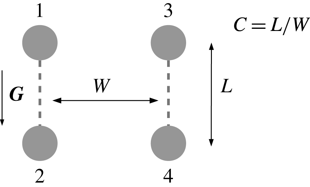
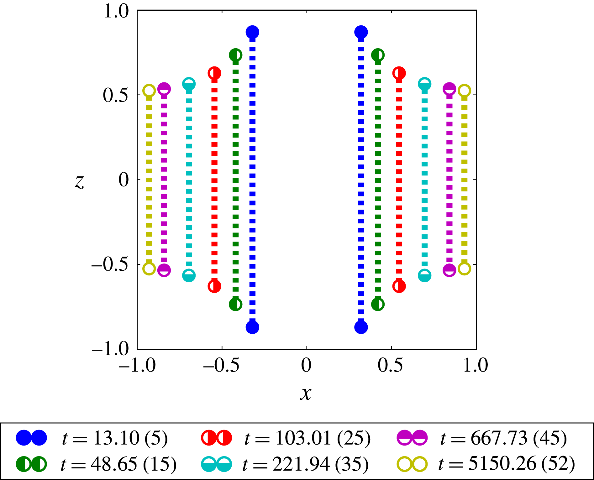
Initially, the dumbbells are oriented vertically, with their centres aligned horizontally, as illustrated in figure 1. The distance
 $L_{in}\equiv L(t=0)$
between the beads within dumbbells is equal to
 $L_{0}$
or
 $1.7L_{0}$
, and the distance
 $W_{in}\equiv W(t=0)$
between the centres of dumbbells spans a range of values determined by the configuration aspect ratio
 $0.9\leqslant C_{in}\equiv L_{in}/W_{in}\leqslant 1.8$
.
The characteristic ‘vertical’ configuration of dumbbells considered in this work.

We assume that the Reynolds number is much smaller than unity. In this case, the bead velocity relaxation time
 ${\it\tau}=m/{\it\zeta}$
, estimated as the bead mass
 $m$
divided by its friction coefficient
 ${\it\zeta}=6{\rm\pi}{\it\eta}a$
, is much smaller than the hydrodynamic time scale, determined by the ratio of the bead radius and its velocity; inertia is irrelevant. The total force (the sum of the hydrodynamic and the external forces) exerted on each bead vanishes. Therefore, the bead velocities are determined by their positions.
In the low-Reynolds-number regime, the fluid velocity
 $\boldsymbol{v}(\boldsymbol{r})$
and pressure
 $p(\boldsymbol{r})$
satisfy the Stokes equations. In general, they are solved with specific boundary conditions imposed on the bead surfaces (typically, it is assumed that the fluid sticks to the solid surfaces of the beads) and at the system boundaries. In our case, there is no ambient flow, the fluid is unbounded and motionless at infinity. The resulting motion of the beads is sometimes called the Stokesian dynamics. It is often determined by the multipole expansion (see Felderhof Reference Felderhof1988), which can be interpreted as multiple ‘reflections’ (see Kim & Karrila Reference Kim and Karrila2005) or ‘scatterings’ (see Felderhof Reference Felderhof1988) of the flow by the bead surfaces. We use the standard dumbbell model, in which the spring is attached to the bead centres. Within this model, there is no external torques exerted on the particles. Therefore, according to the classical mobility problem based on the Stokes equations, see e.g. Felderhof (Reference Felderhof1988) or Kim & Karrila (Reference Kim and Karrila2005), time derivatives of the bead positions, equal to components of their translational velocities, are sums of the corresponding translational–translational mobility coefficients multiplied by the components of the external forces
 $\boldsymbol{F}_{i}$
exerted on each bead
 $i$
, see (2.1)–(2.3). The mobility coefficients and the external forces depend on the bead relative positions, but do not depend on their orientations. Owing to this property, it is possible to determine the translational motion of the beads by solving the system of ordinary differential equations (ODEs) for their time-dependent positions. This can be done without knowing anything about the time-dependent particle orientations: translational motion is decoupled from the rotational motion.
In this work, the distances between any bead centres are much larger than the bead radius
 $a$
. The dumbbell length is at least 10 times larger than
 $a$
. The distances between the centres of the beads forming different dumbbells are also significantly larger than the bead radius. All the beads are spaced well-apart. Therefore, the point-particle approximation is justified.
In the presence of point particles, see e.g. Kim & Karrila (Reference Kim and Karrila2005), the fluid velocity
 $\boldsymbol{v}(\boldsymbol{r})$
and pressure
 $p(\boldsymbol{r})$
satisfy the Stokes equations with the additional sum of the point forces, located at the centres of the beads
 $\boldsymbol{r}_{\boldsymbol{i}}$
,
 $i=1,\dots ,4$
,
 $$\begin{eqnarray}\displaystyle & \displaystyle {\it\eta}{\rm\nabla}^{2}\boldsymbol{v(r)}-\boldsymbol{{\rm\nabla}}p(\boldsymbol{r})=-\mathop{\sum }_{i=1}^{4}\boldsymbol{F}_{i}{\it\delta}(\boldsymbol{r}-\boldsymbol{r}_{\boldsymbol{i}}), & \displaystyle\end{eqnarray}$$
 $$\begin{eqnarray}\displaystyle & \displaystyle \boldsymbol{{\rm\nabla}}\boldsymbol{\cdot }\boldsymbol{v(r)}=0. & \displaystyle\end{eqnarray}$$
 $\boldsymbol{v}(\boldsymbol{r})$
and
 $p(\boldsymbol{r})$
follow as superpositions of the corresponding Green tensors
 $\unicode[STIX]{x1D642}(\boldsymbol{r}-\boldsymbol{r}_{\boldsymbol{i}})$
, contracted with the forces
 $\boldsymbol{F}_{i}$
,
 $i=1,\dots ,4$
. For velocity,
 $\unicode[STIX]{x1D642}$
is the Oseen tensor
 $\unicode[STIX]{x1D64F}(\boldsymbol{r})$
,
 $$\begin{eqnarray}\unicode[STIX]{x1D64F}(\boldsymbol{r})=\frac{1}{|\boldsymbol{r}|}\left(\unicode[STIX]{x1D644}+\frac{\boldsymbol{r}\otimes \boldsymbol{r}}{|\boldsymbol{r}|^{2}}\right).\end{eqnarray}$$
Here and later on, we use dimensionless variables, based on
 $L_{0}$
as the length unit,
 $G/(8{\rm\pi}{\it\eta}L_{0})$
as the velocity unit, and
 $G$
as the force unit. Therefore,
 $8{\rm\pi}{\it\eta}L_{0}^{2}/G$
is the time unit, and
 $G/L_{0}$
is the unit of the spring constant.
In the point-particle model, each bead is advected by the superposition of the fluid flows generated by all the other point-like beads, plus a self-term, proportional to the single-particle mobility and the external force. Therefore, velocity
 $\boldsymbol{V}_{i}$
of particle
 $i$
has the form
 $$\begin{eqnarray}\boldsymbol{V}_{i}=\frac{4}{3a}\boldsymbol{F}_{i}+\mathop{\sum }_{j\neq i}\unicode[STIX]{x1D64F}(\boldsymbol{r}_{ij})\boldsymbol{\cdot }\boldsymbol{F}_{j}.\end{eqnarray}$$
Positions
 $\boldsymbol{r}_{i}$
of beads
 $i=1,\dots ,4$
as functions of time are determined by the set of ODEs
 $$\begin{eqnarray}\displaystyle \frac{\text{d}\boldsymbol{r}_{i}}{\text{d}t}=\boldsymbol{V}_{i}. & & \displaystyle\end{eqnarray}$$
In (2.7), the bead radius enters only into the self-term, through the single-bead mobility coefficient. In the absence of elasticity, a frame of reference moving with a single bead can be chosen, i.e. with velocity
 $G/(6{\rm\pi}{\it\eta}a)$
. In this frame, the dynamics does not depend on the bead radius, see Ekiel-Jeżewska (Reference Ekiel-Jeżewska2014). This means that the relative motion does not depend on the bead radius. However, in the presence of the time-dependent spring forces
 $\boldsymbol{ S}_{i}$
, such a reasoning cannot be applied. Taking into account that
 $S\ll G$
(as will be explained in § 3.4) we conclude that in the presence of elastic forces, the relative motion of the beads depends on
 $a$
, but this effect is very small.
The equations of motion (2.7)–(2.8) are solved numerically using the fourth-order adaptive Runge–Kutta method. When solving, we impose the symmetry of the dumbbell configurations with respect to reflection in the vertical plane
 $x=0$
, and we keep the centres of the beads in the plane
 $y=0$
.
3. Results
3.1. Basic features of the dynamics
Before analysing the dynamics of the system of two dumbbells, we first discuss the motion of a single dumbbell. Equations (2.7) and (2.8) lead to the conclusion that a single elastic dumbbell keeps its initial orientation all the time, and its off-equilibrium length
 $L_{s}$
monotonically approaches the equilibrium value
 $L_{0}=1$
. The time-dependence of the dumbbell length
 $L_{s}$
follows from the relation,
 $A|L_{s}-1|\left(L_{s}-(3a/2)\right)^{-3a/2}=\text{exp}[-(4k(2-3a)/3a)t],$
where the constant
 $A$
is determined by the initial extension of the spring
 $L_{s,in}-1\neq 0$
, with
 $L_{s,in}\geqslant 2a$
. For small deviations from the equilibrium and small bead radii, the time scale of the exponential decay
 ${\it\tau}\approx 3a/(8k)$
.
Now we move on to discuss the dynamics of the system of two dumbbells, introduced in § 2.
Assume that initially four beads are placed at the corners of a vertical rectangle as shown in figure 1, and consider pairs of the beads 1–2 and 3–4 as ‘dumbbells’. Let us first discuss the dynamics for
 $k=0$
, i.e. for separate beads without any constraint forces, analysed by Hocking (Reference Hocking1963) and Tory, Kamel & Tory (Reference Tory, Kamel and Tory1991) and shown as videos by Ekiel-Jeżewska & Sikora (Reference Ekiel-Jeżewska and Sikora2010), and for
 $k=\infty$
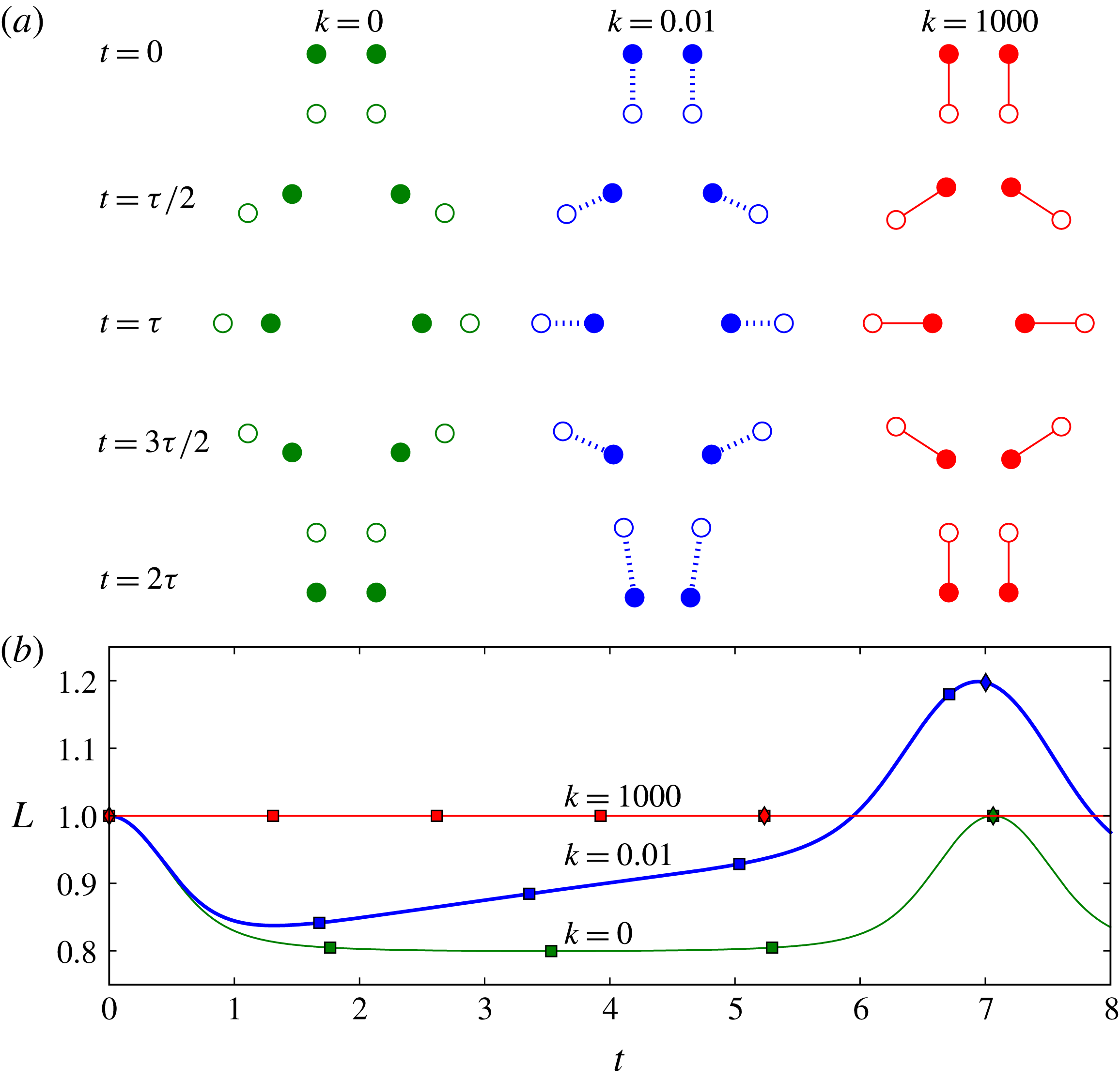
, i.e. for two rigid dumbbells, which model rods, investigated by Jung et al. (Reference Jung, Spagnolie, Prikh, Shelley and Tornberg2006). At the initial configuration hydrodynamic interactions between the beads lead to contraction of the upper side of the rectangle and elongation of the bottom one, so an isosceles trapezoid is formed. Then, the upper side expands a bit, while the bottom side expands even more. The beads from the upper side move faster than the others, the height of the trapezoid monotonically diminishes and the dumbbells rotate. At the same time, hydrodynamic interactions lead to drifting apart of the right and left dumbbells and the trapezoid expands in the horizontal direction. For
 $k=0$
, the dumbbell length
 $L$
shrinks, while for
 $k=\infty$
, it is constant. After a certain time
 ${\it\tau}$
, the trapezoid flattens to a single horizontal line and the largest horizontal distance between the beads reaches the maximum.
For larger times,
 ${\it\tau}+t$
, the particle positions coincide with the earlier positions of the particles at time
 ${\it\tau}-t$
, reflected in the horizontal plane in which all the particles are located at time
 ${\it\tau}$
. This property follows from the symmetry of the Stokes equations with respect to time reversal, as explained e.g. by Caflisch et al. (Reference Caflisch, Lim, Luke and Sangani1988). Therefore, the internal beads move faster than the external ones and an upside-down trapezoid is formed. The left and right dumbbells rotate and approach each other, and after the tumbling time
 $2{\it\tau}$
they again form the initial rectangle, but with the flipped dumbbells: now beads 2 and 4 are at the top, see the left and right plots of figure 2(a).
Evolution of pairs of separate beads (
 $k=0$
), elastic dumbbells (
 $k=0.01$
) and almost rigid dumbbells (
 $k=1000$
), for
 $a=0.1$
,
 $C_{in}=1.0$
and
 $L_{in}=1.0$
. (a) Snapshots taken at equal time intervals
 ${\it\tau}/2$
(equal to 1.8 for
 $k=0$
, 1.7 for
 $k=0.01$
and 1.3 for
 $k=1000$
). (b) Evolution of the dumbbell length
 $L$
, with squares corresponding to the snapshots, and diamonds to vertical configurations. For
 $k=0.01$
, the motion is not periodic.

Basic features of this tumbling dynamics are also recovered by sedimenting elastic dumbbells as they move from a vertical configuration to a horizontal one and vice versa. The essential difference is that, owing to the presence of the elastic forces (2.3), there is no symmetry between the relative motion of the beads at
 ${\it\tau}-t$
and
 ${\it\tau}+t$
. Therefore, there is no periodicity of the relative positions, and consecutive tumbling times are not equal to each other. In figure 2(a), the lack of symmetry is evident in the middle plot, where the initial vertical dumbbell configuration at
 $t=0$
is not reproduced at
 $t=2{\it\tau}$
. It is also clearly visible in figure 2(b) as the non-symmetric curve of the time-dependent dumbbell length
 $L$
for
 $k=0.01$
. In particular, the second vertical configuration on this curve (marked by the last diamond) corresponds to time larger than
 $2{\it\tau}$
(marked by the last square). For comparison, we also show the symmetric curve for separate beads (
 $k=0$
), and the almost constant curve for
 $k=1000$
, to illustrate that such a dumbbell can in practice be considered as rigid; indeed, in this case
 $L$
changes by
 $3\times 10^{-5}$
only.
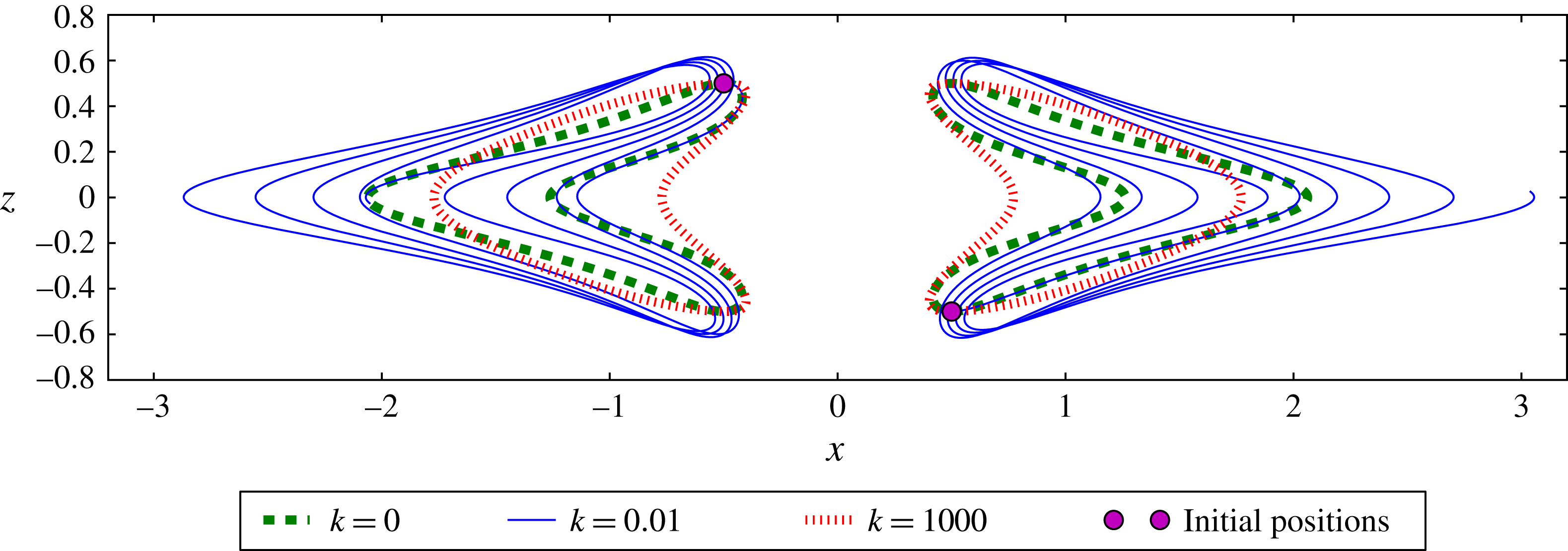
It is convenient to analyse the influence of elasticity on the motion, using the centre-of-mass reference frame, so periodicity is easily visible as closed trajectories. In figure 3, we plot the centre-of-mass trajectories of two beads from different dumbbells. For
 $k=1000$
(dotted line) the trajectories, plotted for 16 tumbling times, are practically closed, and their shape is qualitatively similar (but not identical) to the closed trajectories of the periodic motion of separate beads (
 $k=0$
, dashed line). Beads of the elastic dumbbells (
 $k=0.01$
, solid line) perform a non-periodic motion and their trajectories are not closed. Until the second tumbling, the trajectories stay close to their analogues for
 $k=0$
and
 $k=1000$
, but later they systematically deviate from the periodic shapes and become wider, as shown in figure 3. The widening of trajectories has been observed during the whole time of simulations and for all intermediate values of
 $k$
, so it seems to be an intrinsic property of the studied system. The widening is correlated with the increase of the trajectory length between subsequent tumbling times, increase of the tumbling time, and increase of the maximal horizontal distance between the dumbbells, reached at their horizontal orientations.
3.2. Relaxation to a universal trajectory
As the motion of elastic dumbbells is not periodic, the parameters
 $C$
,
 $L$
and
 $W$
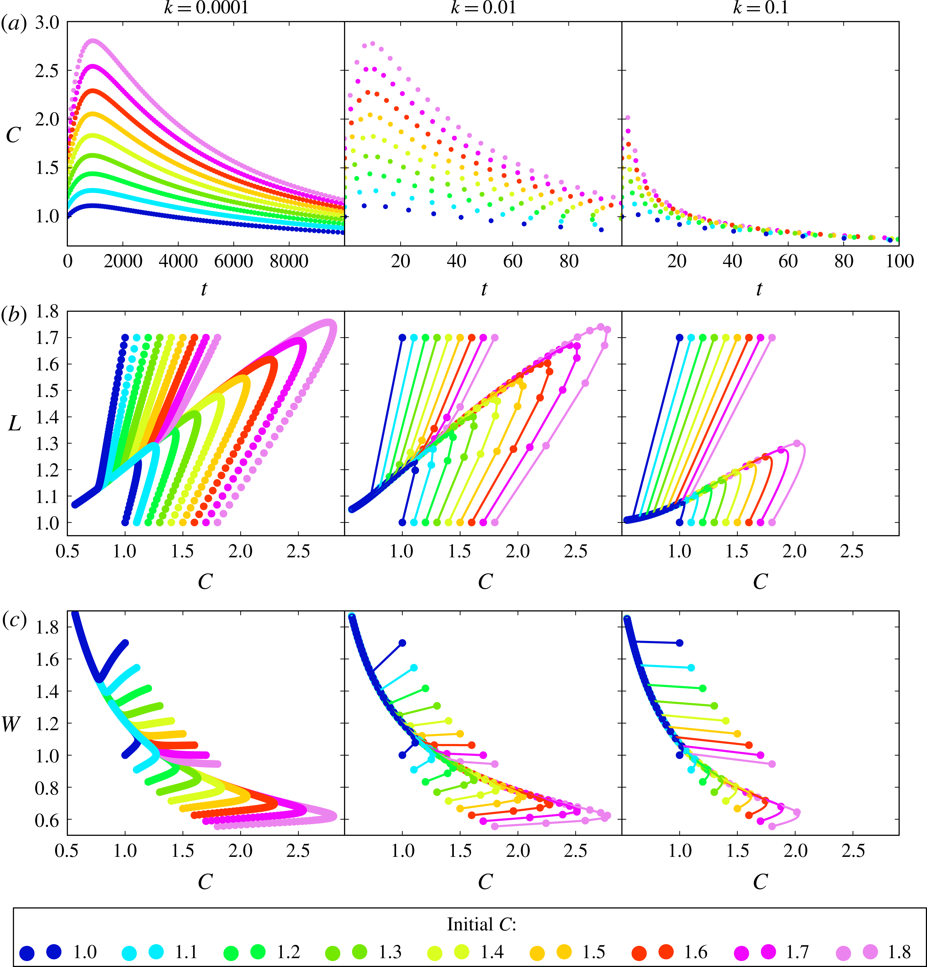
, measured in vertical configurations (shown in figure 1), change over time and can be used to describe evolution of the dynamics. The results are shown in figure 4. Here, the simulation time
 $t=10\,000$
and
 $a=0.1$
. Two main phases of the dynamics are clearly visible. For a given
 $k$
, the system converges to a single universal time-dependent solution.
Trajectories of two beads from different dumbbells, in the centre-of-mass reference frame (drawn to scale). They are closed (periodic) for separate beads and rigid dumbbells, but non-closed (non-periodic) for elastic dumbbells. Here,
 $a=0.1$
,
 $C_{in}=1$
,
 $L_{in}=1$
.

The system relaxation to a universal time-dependent solution. The dots represent consecutive vertical configurations with time-dependent aspect ratio
 $C$
, height
 $L$
and width
 $W$
. (a) Evolution of
 $C$
(for
 $L_{in}=1$
); (b)
 $L$
versus
 $C$
(for
 $L_{in}=1$
or 1.7); (c)
 $W$
versus
 $C$
(for
 $L_{in}=1$
or 1.7).

In figure 4(a), the time-dependent aspect ratio
 $C$
of various vertical configurations with
 $L_{in}=1$
is shown. During the first phase, the value of
 $C$
rises. The relaxation occurs, since the state when vertical dumbbells keep their equilibrium length
 $L_{0}$
does not seem to be ‘natural’ for the studied system. As illustrated in figure 2(b), elastic dumbbells tend to be stretched in vertical orientations. In the second phase, the value of
 $C$
monotonically decreases and approaches a
 $k$
-specific limit,
 $C_{0}$
. The stiffer the dumbbells are, the shorter the relaxation time is, as shown in figure 4(a) (note different time scales displayed at different values of
 $k$
). This behaviour is observed for
 $0.0001\leqslant k\leqslant 1$
.
To investigate the dynamics after the relaxation time in figures 4(b) and 4(c) we plot
 $L$
versus
 $C$
and
 $W$
versus
 $C$
, measured at consecutive vertical configurations. The essential feature following from these plots is that all the initial vertical configurations converge to a single, universal trajectory.
Independently of the initial values
 $L_{in}$
of the dumbbell length, and
 $C_{in}$
of the system aspect ratio, after a certain relaxation time,
 $C$
monotonically decreases in consecutive vertical configurations. Then, the evolution of the trajectories
 $W(C)$
and
 $L(C)$
is the same and depends only on the spring constant
 $k>0$
. The same vertical configurations lead to identical, universal time-dependent evolution in between. Relaxation of the system, clearly visible in figure 4(b,c), takes place on a time scale which can be estimated from figure 4(a).
3.3. Hydrodynamic repulsion
From figure 4 it follows that in consecutive vertical configurations of the universal trajectory, the distance
 $W$
between the dumbbells increases with time. This behaviour can be interpreted as an effective horizontal repulsion of elastic dumbbells, caused by their hydrodynamic interactions. The effect is clearly visible in figure 5, where relative positions of the beads are shown in successive (but not consecutive) vertical configurations. Systematically, for a larger time, the distance between vertically oriented dumbbells is larger. The hydrodynamic repulsion can be significant; e.g. as illustrated in figure 4, it can lead to a tripling of the distance
 $W$
between the dumbbells in vertical configurations. The speed of the repulsion is largest for
 $k=0.01{-}0.1$
.
Snapshots of elastic dumbbells in successive vertical configurations, after the indicated time and number of flips. The dumbbells move away from each other during the motion. Here,
 $k=0.01$
,
 $a=0.1$
,
 $C_{in}=1.8$
and
 $L_{in}=1.0$
. For the sake of clarity, the bead size is reduced by a factor three.

More information about hydrodynamic repulsion and other features of the dynamics of two sedimenting elastic dumbbells can be found in two online supplementary movies available at http://dx.doi.org/10.1017/jfm.2015.31, which illustrate the motion in the centre-of-mass reference frame. The evolution of two initial aspect ratios,
 $C_{in}=1$
and
 $C_{in}=1.8$
, is shown for two values of the spring constant,
 $k=0.01$
and
 $k=0.1$
. Initially, the dumbbells have the equilibrium length
 $L_{in}=1$
, but it is clearly visible that their length
 $L$
changes with time while the dumbbells tumble. This effect is pronounced for
 $C_{in}=1.8$
and
 $k=0.01$
.
At the beginning, the dumbbell length
 $L$
at consecutive vertical positions increases with time. This behaviour corresponds to the relaxation phase, in agreement with figure 4. Later, when the universal trajectory is approached, the value of
 $L$
at consecutive vertical positions decreases monotonically. For
 $C_{in}=1.8$
, the initial horizontal distance
 $W_{1}$
between vertical dumbbells is much smaller than
 $W_{2}$
in the case of
 $C_{in}=1$
. Therefore, the universal trajectory is approached at a smaller value of
 $W_{1}$
, and more time is needed for the system to reach the larger value
 $W_{2}$
. Comparing the movies for
 $C_{in}=1.8$
and
 $C_{in}=1$
, we can observe that along the universal trajectory, the tumbling time significantly increases when
 $W$
evolves and becomes larger. In our movies, the largest speed of the hydrodynamic repulsion is observed for
 $k=0.1$
and
 $C_{in}=1.8$
. This effect results from an interplay of the corresponding slopes of the
 $W(C)$
and
 $C(t)$
curves in the relevant regimes.
Along the universal trajectory, the parameter
 $C$
decreases with time; this change leads to universal patterns of trajectory widening, including the increase of its length and the maximal horizontal size
 $d_{max}$
. An analogous dependence of the trajectory width and the tumbling time on the parameter
 $C$
was observed by Ekiel-Jeżewska (Reference Ekiel-Jeżewska2014) for a wider class of regular systems of separate beads.
3.4. How large are elastic forces in comparison to gravity?
The significant hydrodynamic repulsion effect shown in figure 5 is entirely due to elastic forces between the beads which form a dumbbell (it is absent in the case of rigid constraints or separate beads). Therefore, in this section we investigate how large are the elastic forces
 $S$
in comparison to gravity
 $G$
. As shown in (2.3),
 $S$
is proportional to the deviation of the spring length from its equilibrium value,
 $r_{12}-L_{0}$
. This quantity depends on the system dynamics, i.e. evolution of all the bead positions. While evolving, the system adjusts these positions in a way which depends on all the system parameters (in particular, also on the bead radius).
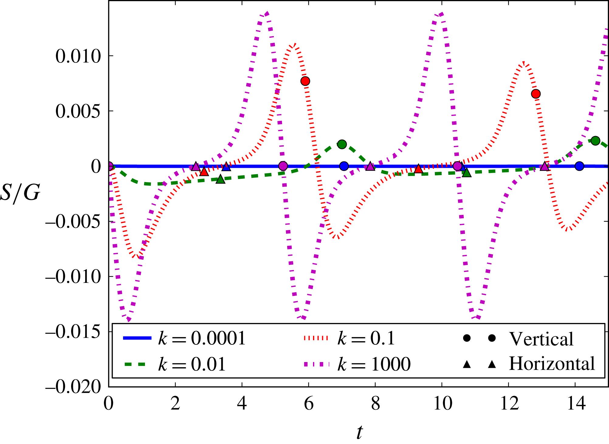
It is remarkable that a large hydrodynamic repulsion is observed even though the elastic force is an order of magnitude smaller than gravity, as we discuss below. The following arguments are valid in the case of the bead radius
 $a\ll r$
, where
 $r$
is the distance between beads. The velocity of bead with the label 1 is given by
 $$\begin{eqnarray}\boldsymbol{V}_{1}=\frac{4}{3a}(\boldsymbol{S}_{1}+\boldsymbol{G})+\unicode[STIX]{x1D64F}(\boldsymbol{r}_{13})\boldsymbol{\cdot }(\boldsymbol{G}+\boldsymbol{S}_{3})+\unicode[STIX]{x1D64F}(\boldsymbol{r}_{14})\boldsymbol{\cdot }(\boldsymbol{G}+\boldsymbol{S}_{4})+\unicode[STIX]{x1D64F}(\boldsymbol{r}_{12})\boldsymbol{\cdot }(\boldsymbol{G}+\boldsymbol{S}_{2}).\end{eqnarray}$$
The velocity of bead 2 of the same dumbbell is easily obtained from (3.1) by the replacements:
 $1\rightarrow 2,2\rightarrow 1$
. The maximum value of elastic force
 $S=k(L-L_{0})$
is reached when
 $\text{d}L/\text{d}t=0$
, i.e. when the relative translational velocity of the beads of each dumbbell has a vanishing component parallel to the dumbbell. (In general, the maximum does not occur for vertical configurations.) After rearrangement we obtain
 $$\begin{eqnarray}\displaystyle & & \displaystyle \hat{\boldsymbol{r}}_{12}\boldsymbol{\cdot }(\boldsymbol{V}_{2}-\boldsymbol{V}_{1})=\hat{\boldsymbol{r}}_{12}\boldsymbol{\cdot }\left[S\frac{-8}{3a}\hat{\boldsymbol{r}}_{12}-G\left(\unicode[STIX]{x1D64F}(\boldsymbol{r}_{23})+\unicode[STIX]{x1D64F}(\boldsymbol{r}_{24})-\unicode[STIX]{x1D64F}(\boldsymbol{r}_{13})-\unicode[STIX]{x1D64F}(\boldsymbol{r}_{14})\right)\boldsymbol{\cdot }\hat{\boldsymbol{z}}\right.\nonumber\\ \displaystyle & & \displaystyle \quad \left.+\,S\left(2\unicode[STIX]{x1D64F}(\boldsymbol{r}_{12})\boldsymbol{\cdot }\hat{\boldsymbol{r}}_{12}+\unicode[STIX]{x1D64F}(\boldsymbol{r}_{23})\boldsymbol{\cdot }\hat{\boldsymbol{r}}_{34}-\unicode[STIX]{x1D64F}(\boldsymbol{r}_{24})\boldsymbol{\cdot }\hat{\boldsymbol{r}}_{34}-\unicode[STIX]{x1D64F}(\boldsymbol{r}_{13})\boldsymbol{\cdot }\hat{\boldsymbol{r}}_{34}+\unicode[STIX]{x1D64F}(\boldsymbol{r}_{14})\boldsymbol{\cdot }\hat{\boldsymbol{r}}_{34}\right)\vphantom{\frac{-8}{3a}}\right]=0.\nonumber\\ \displaystyle & & \displaystyle\end{eqnarray}$$
On the right-hand side of (3.2), the first and the third terms are proportional to the elastic forces
 $S$
. The first term scales as
 ${\sim}(1/a)$
and the following ones scale as
 $T(\boldsymbol{r})\sim (1/r)$
. Therefore, for
 $a\ll r$
, the third term can be neglected. Given that the relative translational velocity of the beads along the dumbbell vanishes, we obtain
 $(|S|/a)\sim (G/r)\Rightarrow (|S|/G)\sim (a/r)\ll 1$
, so when the bead radius is small, the maximal value of elastic force is much smaller than gravity. Figure 6 illustrates that in our simulations with
 $a\leqslant 0.1$
, the elastic forces are indeed much weaker than gravity. For
 $a\ll r$
, by neglecting the third term in (3.2), we obtain the approximate dynamics which depends on the spring constant
 $k$
and the bead radius
 $a$
only through the ratio
 $k/a$
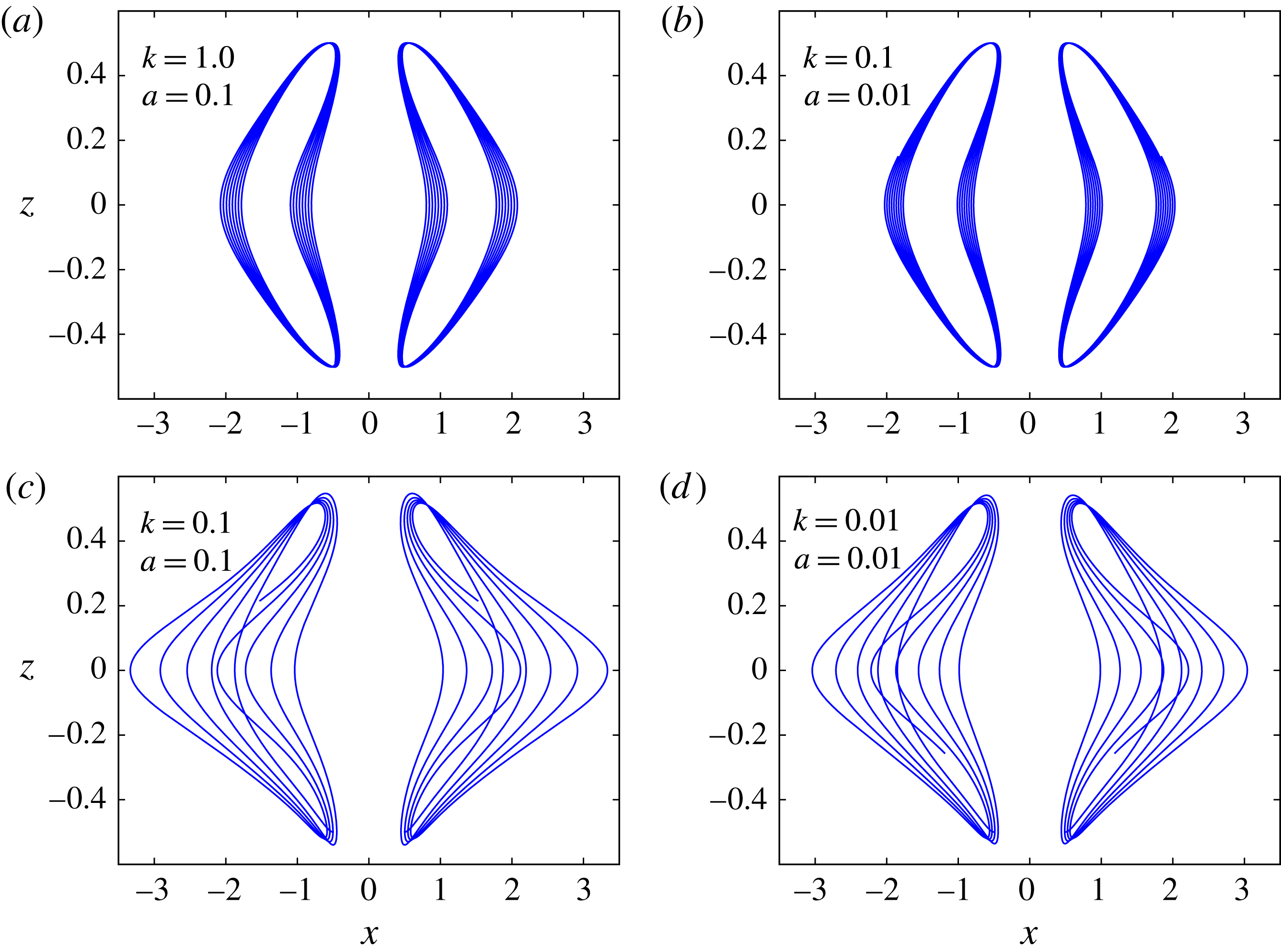
. The applicability of this approximation is consistent with our observations of trajectories with
 $r\sim 1$
in the centre-of-mass reference frame for different values of
 $k$
and
 $a\leqslant 0.1$
, shown in figure 7. The beads trajectories corresponding to the same ratio
 $k/a$
are almost the same.
The time-dependent ratio
 $S/G$
of the elastic to gravitational forces is shown to be much smaller than one. Symbols: vertical and horizontal dumbbell configurations.

Trajectories of dumbbell beads in the centre-of-mass reference frame are in practice determined only by the ratio
 $k/a$
, provided that
 $a\ll 1$
. (a,b) Different values of
 $k$
, but the same ratio
 $k/a=10$
; (c,d) different values of
 $k$
, but the same ratio
 $k/a=1.0$
.

3.5. Critical value of the aspect ratio
 $C$

Vertical configurations with
 $W$
much greater than
 $L$
(i.e. with very small aspect ratios
 $C=L/W$
) do not lead to the dumbbell tumbling. For elastic dumbbells, similarly to the case of separate beads, described by Hocking (Reference Hocking1963) and Ekiel-Jeżewska (Reference Ekiel-Jeżewska2014), there exists a critical value
 $C_{0}\approx 0.55$
. For
 $C<C_{0}$
, there is no tumbing and the motion of the dumbbells decouples. They move away from each other with a decreasing velocity, and finally each of them tends to behave as a single dumbbell.
For separate beads, an approximate analytic solution close to the critical point
 $C=C_{0}$
was derived by Ekiel-Jeżewska (Reference Ekiel-Jeżewska2014). It was shown that for
 $C>C_{0}$
oscillations appear, but for
 $C<C_{0}$
they are absent. For two elastic dumbbells, the critical value of
 $C_{0}$
is of the same order as for four separate beads. This result could be associated with small values of the elastic forces in comparison to gravity, in agreement with the conclusions from § 3.4.
4. Discussion and concluding remarks
In this work we report the novel finding of horizontal hydrodynamic repulsion of two elastic dumbbells which settle under gravity in a viscous fluid. The general remark following from our point-particle simulations is that the replacement of rigid links between the dumbbell beads by elastic springs significantly changes the dynamics. The periodic tumbling, observed by Jung et al. (Reference Jung, Spagnolie, Prikh, Shelley and Tornberg2006) for two rigid sedimenting dumbbells, is replaced by a more complex pattern of non-periodic oscillations when elastic dumbbells are initially located in the same configuration. In the limit of vanishing spring constant
 $k$
, when there are no constraints, we recover periodic tumbling, found by Hocking (Reference Hocking1963). The striking effects of elasticity are observed even though the elastic forces are very small in comparison to gravity (as demonstrated in § 3.4).
We have shown that for each value of
 $k$
, there exists a universal time-dependent solution to which the system dynamics converges, as displayed in figure 4. We have discovered an increase of the distance between the elastic dumbbells in their consecutive vertical configurations (shown in figure 5), correlated with the systematic increase of the trajectory width (visible in figure 3) at times corresponding to horizontal orientations of the dumbbells. The dumbbell length oscillates and very slowly tends to its equilibrium value. The maximal distance between dumbbells in vertical configurations is limited by the dumbbell length divided by the critical aspect ratio
 $C_{0}$
; for
 $C<C_{0}$
tumbling motions do not occur. The hydrodynamic repulsion is faster for higher values of
 $C$
, when the tumbling time is shorter. The hydrodynamic repulsion has been also observed for all values of
 $k$
, with the largest speed for
 $k=0.01{-}0.1$
. The behaviour described above takes place for a wide range of values of
 $k$
and
 $a$
, and at the lowest order, it depends only on the ratio
 $k/a$
, of course as long as the point-particle approximation is justified.
The question arises of what is the physical meaning of the dimensionless values of the spring constant,
 $k=0.1$
and
 $k=0.01$
, for which the maximum repulsion effect is observed between sedimenting dumbbells. For example, let us consider springs made of DNA strands, which were used e.g. by Dreyfus et al. (Reference Dreyfus, Baudry, Roper, Fermigier, Stone and Bibette2005) to construct artificial microswimmers. Within the Hookean regime, the spring constant of a DNA chain was measured e.g. by Bustamante et al. (Reference Bustamante, Smith, Liphardt and Smith2000), with values equal to
 $10^{-6}{-}10^{-5}~\text{pN}~\text{nm}^{-1}$
corresponding to decreasing the chain length from 100 to
 $10~{\rm\mu}\text{m}$
. Constructing the dumbbells from
 $50~{\rm\mu}\text{ m}$
long strands of DNA, and beads twice as dense as water and radii around
 $5~{\rm\mu}\text{m}$
, we recover values of the dimensionless spring constant in the range
 $k=0.01{-}0.1$
.
The mechanism of the observed convergence to the universal solution will be analysed elsewhere for a more general system of many elastic dumbbells.
Acknowledgement
This work was supported in part by the Polish National Science Centre, Grant No. 2011/01/B/ST3/05691. Scientific benefits from the activities of the COST Action MP1106 are acknowledged.
Supplementary movies
Supplementary movies are available at http://dx.doi.org/10.1017/jfm.2015.31.