


1. Introduction
Solar-like stars are composed of an inner radiative zone surrounded by an outer convective envelope, with the photosphere marking the upper boundary of this convective region and the chromosphere lying just above it. These stars exhibit global oscillations, particularly pressure (p) modes, which are stochastically excited and damped by turbulent convection in their outer layers (e.g. Goldreich and Keeley Reference Goldreich and Keeley1977). The properties of these modes are sensitive to small perturbations in the stellar interior, making them powerful diagnostics for probing internal structure. Asteroseismology uses these oscillations to infer fundamental stellar parameters. This requires long, high-precision time series of stellar brightness or radial velocity that capture the surface signatures of the oscillations. By transforming the time series into the frequency domain using Fourier analysis, the power spectral density (PSD) can be computed. In the PSD, pressure modes appear as distinct peaks, whose frequencies, amplitudes, and linewidths provide detailed information about the star’s internal structure and dynamics (García Reference García2015). In addition to their oscillations, solar-like stars display magnetic activity at the surface, with features that vary over a range of spatial and temporal scales. These variations are closely associated with magnetic activity cycles and have measurable effects on the properties of oscillation modes. As magnetic activity increases, mode frequencies tend to rise, while amplitudes and energies decrease (García et al. Reference García, Salabert, Mathur, Régulo and Ballot2013; Salabert et al. Reference Salabert, García and Turck-Chièze2015; Régulo et al. Reference Régulo, García and Ballot2016; Santos et al. Reference Santos, Campante, Chaplin, Cunha and van Saders2019). These changes can affect asteroseismic inferences of stellar properties such as mass, radius, and age (Bétrisey et al. Reference Bétrisey, Broomhall, Breton, García, Davenport and Kochukhov2025). Properly accounting for the influence of magnetic activity is therefore essential, especially in the context of upcoming space missions such as PLAnetary Transits and Oscillations of stars (PLATO) (Rauer et al. Reference Rauer, Aerts, Cabrera, Deleuil and Erikson2025), which are scheduled for launch in December 2026. PLATO aims to detect and characterize terrestrial exoplanets orbiting solar-type stars. Achieving the mission’s science goals will depend on accurately determining the fundamental properties of the host stars, which in turn requires a robust understanding of how magnetic activity affects oscillation modes. Previous helioseismic studies have already revealed unexpected behavior in the Sun’s oscillation spectrum. Data from the InterPlanetary Helioseismology by IRradiance measurements (IPHIR) experiment (Fröhlich et al. Reference Fröhlich, Bonnet, Bruns, Delaboudinière and Domingo1988) aboard the PHOBOS satellite, and from the first 310 days of observations by the Global Oscillations at Low Frequencies (GOLF) instrument (Gabriel et al. Reference Gabriel, Grec, Charra, Robillot and Roca Cortés1995; García et al. Reference García, Turck-Chièze, Boumier, Robillot and Bertello2005) on the Solar and Heliospheric Observatory (SoHO) (Domingo et al. Reference Domingo, Fleck and Poland1995), showed evidence of correlated excitation among low-degree p modes (Baudin et al. Reference Baudin, Gabriel, Gibert, Palle and Regulo1996; Foglizzo Reference Foglizzo1998). Such correlations were unexpected under the assumption of purely stochastic excitation. This led Foglizzo (Reference Foglizzo1998) to propose the existence of an additional excitation mechanism, possibly linked to solar eruptive phenomena such as coronal mass ejections (CMEs), which occur on large spatial scale and are associated to high kinetic energy. Surfaca waves were already observed The Sun, being the most comprehensively observed solar-like star, provides a unique opportunity to investigate these effects in detail. In this study, we revisit the assumption of purely stochastic excitation and explore potential connections between mode energy, magnetic activity, and solar eruptive events. Our analysis is based on more than 28 years of Sun-as-a-star observations from SoHO, covering solar cycles 23, 24, and the first half of cycle 25. This work has been published in Panetier et al. (Reference Panetier, García, Breton, Jiménez and Foglizzo2025) and readers are referred to that paper for a complete description and detailed analysis.
2. Retrieving the energy time-series of the modes
This study makes use of data collected by two instruments on board the Solar and Heliospheric Observatory (SoHO), launched in December 1995. The Sun PhotoMeters of the Variability of Solar Irradiance and Gravity Oscillations (VIRGO/SPM) monitor variations in solar irradiance (Fröhlich et al. Reference Fröhlich, Romero, Roth, Wehrli and Andersen1995), while the Global Oscillations at Low Frequencies (GOLF) measure solar Doppler velocity. We focused on acoustic modes with radial orders between
 $n=14$
and
 $n=25$
and angular degrees
 $\ell=0$
, 1, and 2. The time series for these modes were reconstructed using a technique based on the method described by Foglizzo et al. (Reference Foglizzo, Garcia, Boumier, Charra and Gabriel1998). For each mode, we applied a frequency-domain filter by selecting a 8
 $\mu$
Hz-spectral window, centred on the mode frequency
 $\nu$
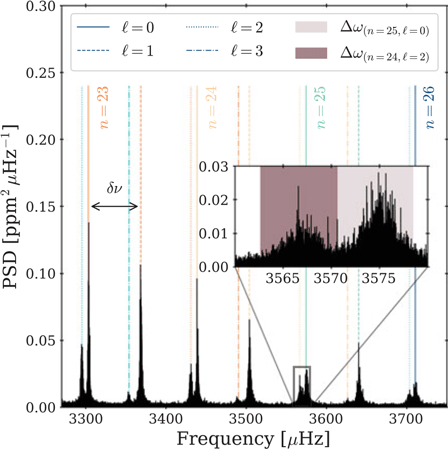
, as identified in the peakbagging analysis of Lazrek et al. (Reference Lazrek, Baudin, Bertello, Boumier and Charra1997). This filtering process is visualized in Figure 1. The mode energy was estimated with the inverse Fourier transform of the filtered signal leading
 $E_{n,\ell} = 2|f_v(t)|^2$
, where
 $f_\nu(t)$
represents the reconstructed time series in the time domain. This approach provides a temporal resolution of roughly 1.45 days. In the subsequent analysis, all mode energy time series were normalized by their respective mean values.
PSD of the VIRGO/SPMs light curve (23.01.1996–23.11.2023) showing frequencies between 3270 and 3750
 $\mu$
Hz, highlighting the large frequency separation (
 $\delta\nu$
) between modes
 $\ell=0$
and
 $\ell=1$
for
 $n=23$
. Modes are marked by vertical lines with colors for
 $n=22$
(light blue),
 $n=23$
(orange),
 $n=24$
(yellow),
 $n=25$
(cyan), and
 $n=26$
(dark blue); line styles indicate degree:
 $\ell=0$
(solid),
 $\ell=1$
(dashed),
 $\ell=2$
(dotted),
 $\ell=3$
(dot-dashed). Inset shows the
 $8\,\mu$
Hz window used to reconstruct mode energies around (
 $n=25$
,
 $\ell=0$
) and (
 $n=24$
,
 $\ell=2$
).

Figure 1 Long description
Panel: A line graph displays the power spectral density (PSD) of the VIRGO/SPMs light curve from January 23, 1996, to November 23, 2023. The horizontal axis represents frequency in microhertz (μHz) ranging from 3270 to 3750 μHz, and the vertical axis represents PSD in parts per million squared microhertz (ppm^2 μHz^-1). The graph highlights the large frequency separation (δν) between modes with vertical lines indicating different modes. Colors denote different radial orders (n=22 in light blue, n=23 in orange, n=24 in yellow, n=25 in cyan, and n=26 in dark blue). Line styles indicate the degree (ℓ=0 as solid, ℓ=1 as dashed, ℓ=2 as dotted, ℓ=3 as dot-dashed). An inset zooms in on an 8 μHz window around the modes (n=25, ℓ=0) and (n=24, ℓ=2), showing detailed mode energies.
3. Kolmogorov-Smirnov (KS) Statistical tests
If a mode is purely stochastically excited, its energy
 $E_{n,\ell}$
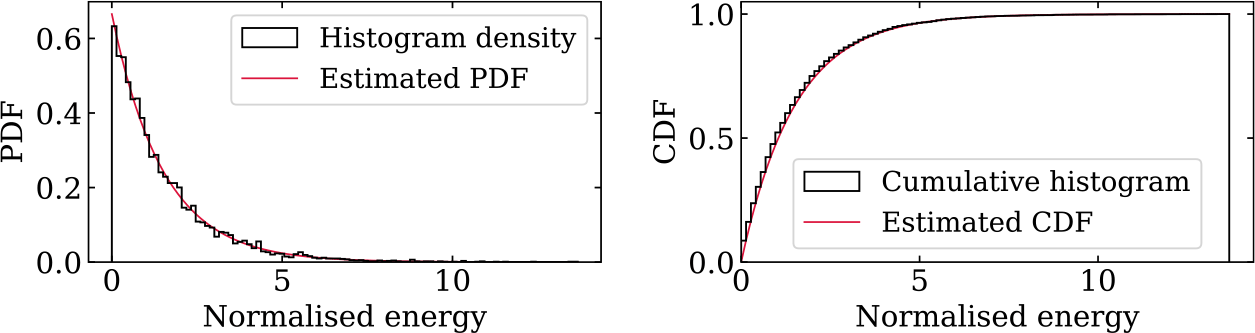
is expected to follow an exponential probability distribution (Chaplin et al. Reference Chaplin, Elsworth, Howe, Isaak, McLeod, Miller and New1997; Foglizzo Reference Foglizzo1998). To evaluate this, we applied the Kolmogorov–Smirnov (KS) test (Massey Reference Massey1951), which compares the empirical cumulative distribution function of the observed energies with that of an ideal exponential distribution. An illustrative example for the mode with
 $n=22$
and
 $\ell=0$
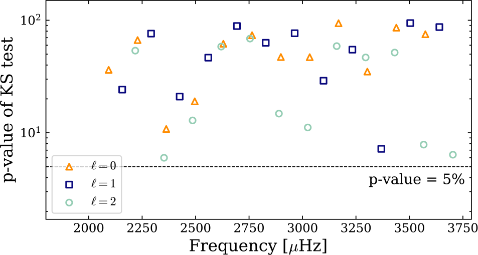
is presented in Figure 2. Figure 3 shows that at a significance level of 5%, all tested time series returned p-values consistent with the null hypothesis, indicating no significant deviation from the expected exponential behavior. These results support the assumption of stochastic excitation for all analyzed modes.
Probability (left) and cumulative (right) distributions for mode
 $n=22$
,
 $\ell=0$
. Black histograms are observed data and red curves show fitted theoretical exponential distributions.

Resulting p-values of the Kolmogorov-Smirnov tests comparing reconstructed time series distributions with exponential distributions. Orange triangles stand for
 $\ell=0$
modes, dark blue squares for
 $\ell=1$
modes, and light blue circles for
 $\ell=2$
modes. The threshold of rejection of 5 % is drawn as a dashed black line

4. The combined energy time-series of the modes
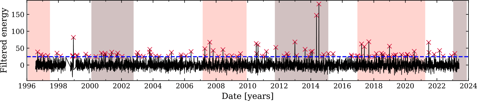
To investigate potential correlations in mode excitation, we combined the 36 reconstructed mode energy time series into a single composite dataset. To account for long-term energy variations caused by solar magnetic activity, the combined time series was normalized by its 1-year moving mean. This produced a normalized time series, denoted
 $S_{\mathrm{phot}}$
, which enhances short-term fluctuations and reveals prominent energy peaks, as shown in Figure 4. Under the assumption of fully stochastic excitation,
 $S_{\mathrm{phot}}$
is expected to follow a
 $\Gamma$
-distribution with shape parameter
 $k=36$
, corresponding to the sum of 36 independent, exponentially distributed mode energies. To test for deviations from this theoretical distribution and assess the influence of magnetic activity, we isolated two sub-samples from
 $S_{\mathrm{phot}}$
corresponding to low and high magnetic activity periods. We compared each sub-sample to the expected
 $\Gamma_{k=36,\mathrm{th}}$
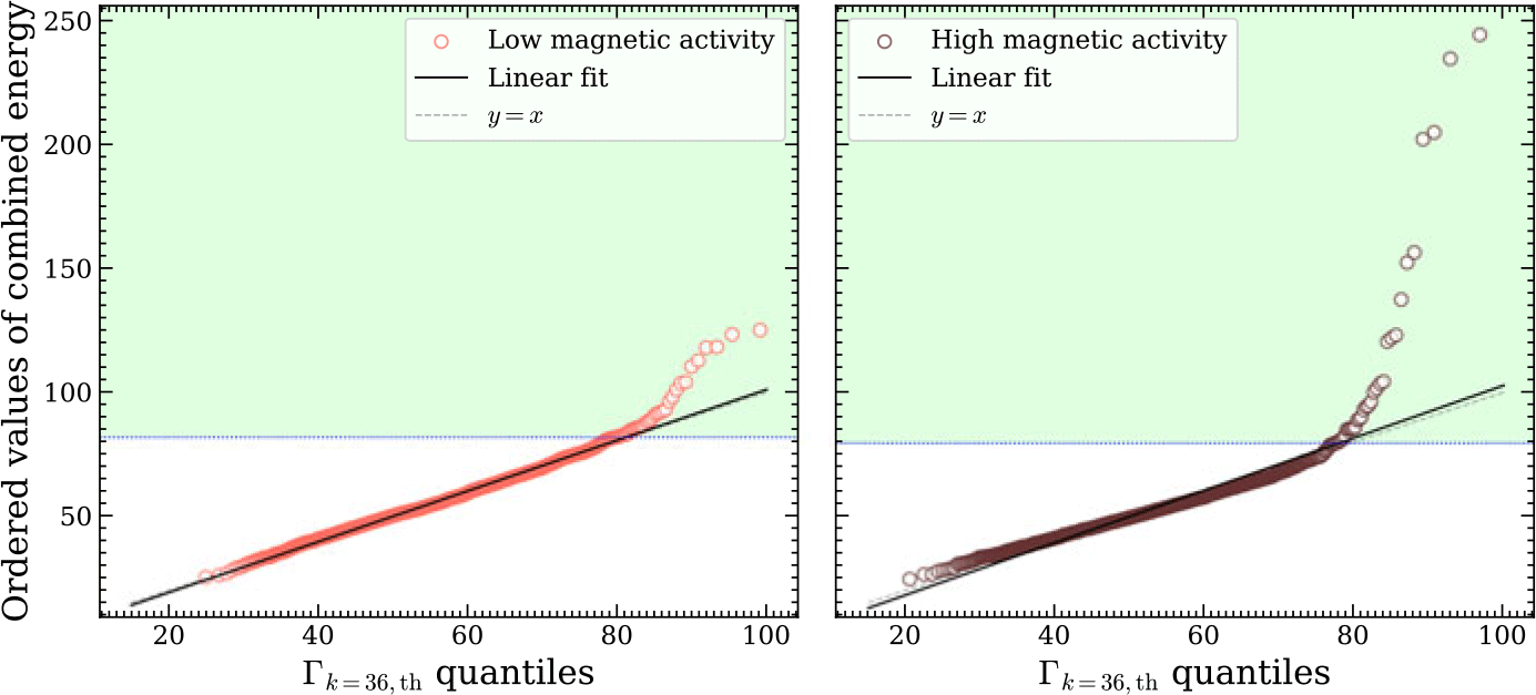
-distribution using quantile–quantile (Q–Q) plots, shown in Figure 5. In both cases, the data deviate from the
 $y = x$
line at high energies, indicating a systematic excess of high-energy events. These discrepancies are similar for both subsets regardless of magnetic activity level. To quantify this excess, we adopted a high-energy threshold corresponding to the 98th percentile of the theoretical distribution. This threshold, indicated by blue dotted lines in Figures 4 and 5, allowed us to identify 108 extreme events out of 6612 data points in
 $S_{\mathrm{phot}}$
. The expected probability of such events occurring purely by chance (
 $P < 10^{-3}$
) is significantly lower than the observed 1.6% rate, confirming their statistical significance and suggesting a departure from purely stochastic excitation.
Combined time series of the 36 analysed modes. This time series was normalised by its one-year moving mean. The blue dashed line shows the 98th percentile and the red crosses mark the studied higher energy points. Periods of low and high magnetic activity, inferred from the solar radio flux index
 $F_{10.7}$
(Tapping Reference Tapping2013) used as a proxy for solar activity, are highlighted in pink and brown, respectively.

Q-Q plot comparing the combined energy time series with
 $\Gamma_{k=36, \mathrm{th}}$
distributions. Panels correspond to two selected sub-samples: low magnetic activity (pink, left) and high magnetic activity (brown, right). The general trend of the Q-Q plot was fitted with a least square regression to the data and is shown as a black line on all panels. The grey dashed line shows the line
 $y=x$
, and the blue dotted line shows the value of the 98th-percentile for each period. The green regions in both panels indicate areas where the observed and theoretical distributions diverge significantly, highlighting their incompatibility.

5. Possible explanations to the excess of energy
To investigate the origin of the observed excess in mode energy, we considered the potential contribution of non-modal disturbances, such as photon noise or transient signals (e.g., particle hits or cosmic rays), which are expected to appear at unrelated frequencies. As a control, we constructed 36 time series using the same temporal windowing as for the modal analysis but shifted by 4500,
 $\mu$
Hz, well outside the p-mode range, to generate a representative noise time series. Comparing the 98th-percentile peaks of this noise series with the 108 high-energy events detected in
 $S_{\mathrm{phot}}$
, we identified 26 coincident peaks likely due to instrumental or environmental noise, leaving 82 events that remain unaccounted for. To examine whether these remaining events are of solar origin, we cross-referenced them with reconstructed time series coming from GOLF observations. This comparison revealed 14 temporal coincidences, suggesting that these events may be linked to intrinsic solar excitation. We further assessed their association with solar eruptive phenomena using a 1.45-day window. Among the 82 unexplained peaks, 22 coincided with coronal mass ejections (CMEs), 8 with solar flares, and only 2 with events also seen in the GOLF data, indicating limited overlap between flare/CME activity and solar-driven mode excitation detectable in both instruments. To explore the excitation depth, we divided the p-mode frequency range into three bands: 2090–2620, 2620–3160, and 3160–3710
 $\mu$
Hz, and reconstructed composite energy time series for each. Within these bands, we found 20, 23, and 28 of the unexplained peaks, respectively, pointing to a modest concentration of energy excess in higher-frequency modes, which are more sensitive to the upper convective layers. However, no significant correlation was observed between the occurrence of these peaks and the solar activity cycle.
6. Conclusions
The primary objective of this study was to examine the influence of surface activity features on mode excitation. Our analysis uncovered deviations from the standard theory of stochastic excitation, revealing that modes are occasionally excited simultaneously at significantly higher rates than predicted. These high-excitation events cannot be fully explained by transient increases in photon noise and do not appear to be directly linked to the solar magnetic cycle. While some events coincide with coronal mass ejections (CMEs) or solar flares, such associations are not systematic. Interestingly, the excess excitation tends to originate more frequently from the outermost layers of the convective zone.
Acknowledgements
The GOLF, VIRGO/SPMs, and LASCO instruments on SoHO represent a collaborative effort between ESA and NASA, with key support from CNES for GOLF. E.P. and R.A.G. thank the GOLF/SoHO and PLATO CNES grants, while S.N.B. acknowledges support from the PLATO ASI-INAF agreement no. 2022-28-HH.0. We also thank the Kepler team, KASC, and NASA for their mission funding. Data from NOAA’s NGDC GOES solar flare X-ray database were used, and we acknowledge Christensen-Dalsgaard et al. (Reference Christensen-Dalsgaard, Dappen, Ajukov, Anderson and Antia1996) for sharing their solar model online.
 μ
 δν
 ℓ=0
 ℓ=1
 n=23
 n=22
 n=23
 n=24
 n=25
 n=26
 ℓ=0
 ℓ=1
 ℓ=2
 ℓ=3
 8μ
 n=25
 ℓ=0
 n=24
 ℓ=2
 n=22
 ℓ=0
 ℓ=0
 ℓ=1
 ℓ=2
 F10.7
 Γk=36,th
 y=x


