

I. Introduction
An integral part of American exceptionalism has been the fact that persons from all walks of life could succeed. Barriers to intergenerational income mobility have historically been perceived to be small. Observers beginning famously with Alexis de Tocqueville and continuing to modern times have spoken of American egalitarianism, manifesting itself in what is often called the American Dream.
With the passage of time, Americans increasingly saw the completion of a good education as being very useful, if not an absolute prerequisite, to the pursuit of economic success. That manifested itself with the common school movement associated with Horace Mann and others, and, with respect to higher education, by government involvement with universities, an effort present since colonial times that increased substantially after the passage of the Morrill Act in 1862 that granted federal lands to the states for the purpose of establishing public universities.Footnote 1 Nonetheless, higher education still remained open only to a small percentage of the population, and the most financially successful men in America before World War II were mostly not college graduates — Cornelius Vanderbilt, John D. Rockefeller, Andrew Carnegie, J. P. Morgan, and Henry Ford are good examples of fabulously wealthy persons with no college background, some of whom (e.g., Rockefeller and Vanderbilt) came from relatively humble family backgrounds.
The GI Bill of 1944 and a frenetic increase in the number and size of universities in the postwar era, however, led to a marked expansion in the number of college graduates, and the development of the view that a college education was a prerequisite for economic success. Beginning with the Higher Education Act of 1965, taxpayer-funded grants and loans became available to low- and middle-income college students, helping to further promulgate the idea that college is the key to social mobility.Footnote 2 While as late as 1970, only about 10 percent of adult Americans had bachelor’s degrees or more, that proportion roughly tripled over the next four decades to around 30 percent, as depicted in Figure 1. This rapid rise in college attainment is attributable to a number of factors, including public policies intended to promote greater attendance, a rising wage differential between college and high school educated workers, and a growing perception that a college degree is necessary for economic success.
U.S. Adult College Attainment Rate, 1940–2011.

It has become an article of faith that higher education is a major vehicle for promoting a path to the middle class and income equality in America. Although those promoting greater government in financing college had done so for many reasons, providing a taxpayer-funded ticket to a middle class, prosperous life to those who cannot afford the cost of attending college as a means to reduce inequality has been a persistent and oft-repeated argument. Both sides of the political aisle have been supportive of these endeavors. For instance, more than 85 percent of the House of Representatives voted in favor of the 1965 Higher Education Act, including 83 percent of the minority Republican members. The bill also easily passed the Senate with 82 percent of the members voting in favor.Footnote 3
The highest-level policymakers in the U.S. government have made proclamations of this nature recently in advocating for greater government support of higher education to promote increased attendance. Speaking at Harvard in 2008, the Chairman of the Federal Reserve Board Ben Bernanke said that “the best way to improve economic opportunity and to reduce inequality is to increase the educational attainment and skills of American workers.”Footnote 4 In pushing to further increase the proportion of adults with college degrees, President Barack Obama, in his 2009 State of the Union address, argued that this “will open the doors of opportunity for our children.”Footnote 5 The Obama Administration reiterated similar claims in its August 2013 higher education policy agenda by declaring that a “college education continues to be the ticket to the middle class.”Footnote 6
In this essay, we explore the economic theory and empirical evidence on the relationship between college attainment and income inequality in the United States, finding that the theoretical relationship is ambiguous and empirical evidence seems to support the existence of a U-shaped inequality-attainment curve. Next is a discussion of related theory, followed by empirical evidence in Section III. The penultimate section offers some policy implications, and Section V concludes.
II. Economic Theory
Advocates for a greater government role in promoting college attendance have often argued that a college education provides greater economic opportunities, and that by reducing inequality of educational opportunity, greater equality of income will follow.Footnote 7 This implies that there is an inverse relationship between inequality of income and the proportion of the population with college degrees. If greater numbers of persons go to college, it is reasoned, the educational and skill advantages previously largely the domain of the richer members of society will expand to a larger segment of the population. With greater educational equality will follow greater economic equality, manifested in a reduced dispersion in the distribution of income.
Policymakers and other public intellectuals espousing such views seem to be echoing the assertions of some academics who have addressed this issue. The most prominent and comprehensive affirmation comes from Claudia Goldin and Lawrence Katz, who observe that income inequality has risen sharply in the United States since 1980, and that this is largely explainable by increasing inequality in the distribution of work-related income.Footnote 8 Economists have often explained this rise in wage inequality as an outcome of skill-biased technological change, hereafter SBTC. The SBTC theory suggests that the incomes of workers with high levels of technological skills rise disproportionately from technological change relative to low skill workers, acting to increase inequality.Footnote 9
Some authors, including Goldin and Katz, contend that the sharp rise in the income differential between high school and college graduates is attributable to SBTC, suggesting that college graduates learn skills that make them better equipped to take advantage of technological change than high school graduates. The implication is that the college-high school income differential is substantially a consequence of inadequate growth in college degree attainment, and that faster growth in college attainment would have spawned greater income equality since more workers would have been equipped to adapt to the technological change that emerged beginning in the 1980s. This argument has been accepted relatively uncritically by several other authors of significant works relating to the economics of higher education in promoting greater equality through an expansion of government finance of higher education.Footnote 10
While SBTC as an explanation for rising inequality may be considered conventional wisdom, a few economists have nonetheless challenged the view that college education imparts the skills necessary to adapt to technological change, showing that rises in educational attainment can lead to greater inequality when education is used by employers as a signaling mechanism. Paul Krugman, for instance, notes that this “could easily be misinterpreted as exogenous skill-biased technological change.”Footnote 11
Building on the screening/signaling theory of Michael Spence,Footnote 12 several authors have constructed models to show that as the number of high ability workers completing a college education rises, the number of high ability workers in the uneducated pool is reduced. Given that wages equal the average expected marginal productivity in equilibrium and education is the only signal of productivity, the average wage level of the uneducated pool declines with a rise in the attainment level. Meanwhile, the pool of educated workers rises along with their average wage level. Such a process would lead to a widening wage differential between the two groups, leading to an increase in inequality. In discussing education as a screening mechanism, Joseph Stiglitz suggested that it “tends to increase inequality.”Footnote 13 Krugman notes: “Anything that encourages good workers to get educated can set in motion a cumulative process of growing inequality.”Footnote 14 Igal Hendel, Joel Shapiro, and Paul Willen show how this process works through policies intended to make college more affordable by reducing credit constraints or subsidizing tuition.Footnote 15
J. B. Knight and R. H. Sabot argue that the overall effect of an increase in educational attainment on inequality depends on the relative strength of the composition and wage compression effects.Footnote 16 The former is the change in inequality resulting from a change in the educational composition of the labor force evaluated at the original educational wage structure, while the latter is the change in inequality resulting from compression of the wage structure evaluated at the original composition. As the relative size of the educated group grows, the compression effect unambiguously generates greater equality while the composition effect initially results in greater inequality, but upon reaching a critical attainment level, additional increases in the attainment rate reduce inequality. The critical attainment rate is higher the lower the education wage premium.Footnote 17 The human capital model of income distribution suggests that an increase in average attainment has an ambiguous effect on inequality, depending on the evolution of rates of return to education.Footnote 18
Most economic theory related to education and inequality has focused on income differences between education groups. Caroline Hoxby and Bridget Terry find, however, that income inequality among college graduates has also grown over time, suggesting that distributional differences both within and between education group contribute to rising income inequality.Footnote 19 The signaling model of Andreas Bergh and Günther Fink, who show that the emergence of private institutions as a means of providing a costly elite signal of ability has an ambiguous effect on inequality as the share of educated workers rises, provides one theoretical avenue through which within-group inequality could rise with the attainment rate if aggregate attainment rates do not account for heterogeneity of the education signal.Footnote 20 This additional dynamic further confounds how increases in college attainment will affect inequality.
Thus, it is not clear a priori what the effect of increasing the college attainment rate will have on income inequality, and empirical evidence has also been mixed.Footnote 21 Nor is it evident that the relationship between the two is linear, as it is possible that the marginal effects depend on the current level of attainment, composition of the labor force and wage structure, and other education-related factors contributing to heterogeneous incomes.Footnote 22 Next we discuss basic economic principles and some rather fundamental observations about human behavior that collectively suggest that in small to medium-sized doses, the notion that greater college attainment promotes income equality is broadly true, but it is clearly untrue when higher education expands beyond a certain point. Pictorially, what may exist is something more like a U-shaped curve that contains both a negatively and positively sloped relationship between higher education attainment and income inequality. This is very similar to a famous graph in economics, the Laffer Curve, which argues that raising tax rates increases tax revenues for a while, but at some point further rate increases become high enough that taxpayers substitute away from production and labor to leisure, shrinking the tax base and reducing tax revenues.
But does a U-shaped inequality-college attainment curve make any sense on broader theoretical grounds? Two basic behavioral realities suggest that the nonlinear, parabolic nature of the equality-higher education relationship makes sense. First, there is a huge gap between the rhetoric of American egalitarianism found in the Declaration of Independence (“all men are created equal”) and elsewhere, and the reality with respect to the innate and acquired abilities of individuals to be economically productive and thus derive income. Cognitive abilities, as measured by IQ tests and other widely used aptitude exams such as the SAT, GRE, and Armed Forces Qualification Test, exhibit a great amount of variation. With economic growth, demand has risen sharply for those possessing cognitive skills relative to those whose “comparative advantage” derives from other skills, especially those requiring physical strength, endurance, or dexterity. Related to this, the ability of students to successfully master higher-order forms of knowledge or critical thinking skills, such as those requiring advanced mathematics, is highly dependent on cognitive ability.
This point ties in with the second behavioral reality: the Law of Diminishing Returns. When university attendance is low, say 5 percent of the population of eighteen- to twenty-two-year-olds, a doubling of that attendance will likely lead many bright persons (with high cognitive skills) to go to college that previously were deprived of that opportunity. Even when 10 percent of the relevant cohort is attending college, most college students are likely to be from the top quartile of the distribution of cognitive skills, and the average IQ of college students may be perhaps 120 — well above the national average of 100. The incremental students benefit hugely from a college education and they generally fulfill relatively high paying jobs requiring university training. When attendance is already very high and a similar 5 percent increase is experienced, from say, 50 percent of the college-aged cohort to 55 percent, by mathematical necessity the number of students admitted of average and even below average levels of cognitive skills rises. The incremental students almost certainly have average IQs of 100 or lower. They are generally far less capable of mastering higher-order skills requiring intellectual rigor. Universities are no longer dominated by, relatively speaking, the cognitively elite. The incremental students no longer generally get high paying jobs that will advance them, and their families, up the economic ladder.
To deal with this situation and avoid massive dropouts, universities offer remedial instruction, lower their grading standards, and water down the curriculum. Students, aware of their academic limitations, increasingly avoid “analytically challenging” subjects such as physics, mathematics, or mechanical engineering, and major in less rigorous subjects such as communication, education, marketing, or recreational management.
Empirical evidence supports this. There is pretty solid evidence that the typical grade point average of undergraduate students has risen from about 2.5 (on a 4 point scale) around 1950 to over 3.0 today, despite the vast increase in the number of students, which almost inevitably required some lowering in the average cognitive abilities of the college-age cohort.Footnote 23 Similarly, the proportion of college students majoring in academically challenging and demanding fields such as the STEM disciplines (science, technology, engineering, and mathematics) has declined. For example, since the mid-1960s, the proportion of college freshmen indicating that they intended to pursue a career in scientific research has fallen by about 50 percent.Footnote 24 Still other evidence suggests that recent college students spend less time on academic pursuits than students did half a century ago — on average, less qualified students work less but receive much higher grades.Footnote 25
We would add that personality traits other than declining average levels of cognitive skills similarly show changes that point in the direction of less rigorous academic preparation. Human beings vary widely in their self-discipline, in their ambition, and in their interest in promoting long-run potential gains to their utility (satisfaction) as opposed to very short-term forms of satisfaction. When college attendance is low, one would suspect that those attending college on average have relatively high quantities of such noncognitive attributes as ambition and a strong work ethic, but as enrollments expand to encompass a majority of the population, that is distinctly less so, particularly as the curricula become less rigorous and require less effort on behalf of the student.
As the proportion of adults with a college degree rises, college completion becomes a less reliable screening device because the ability of employers to predict the likely productivity attributes of college graduates declines as those graduates become less distinctive from the general population. To overcome this challenge, employers begin to use additional criteria to screen applications such as reputation of the university attended and possession of an advanced graduate degree. Students attending elite private colleges or pursuing advanced degrees are likely to be brighter, more industrious, and so on, than those attending nonselective state institutions or those with a terminal bachelor degree. In response, students increasingly pursue admittance to elite private colleges and/or graduate education as a means to enhance their signal to prospective employers.
A good deal of evidence suggests that the perceived quality gap between typical state universities and the elite private institutions has widened a good deal. For example, in 1988, eight of the top twenty-five national universities in the U.S. News and World Report rankings were public universities; today, only three are public. Resources per student have grown faster for the private schools, particularly as state appropriation growth for public universities has slowed significantly from earlier generations. Recipients of Pell Grants are typically from relatively low-income families, and government statistics show that the proportion of Pell Grant recipients at prestigious private schools is dramatically lower than at state schools. For example, at a sample of twenty-five elite private schools that we examined (Harvard, Yale, Princeton, Dartmouth, Columbia, Pennsylvania, Cornell, Brown, Williams, Swarthmore, Pomona, Amherst, M.I.T., Stanford, Duke, Chicago, Northwestern, Notre Dame, Emory, Vanderbilt, Cal Tech, Washington University in St. Louis, Bowdoin, Washington and Lee, and Wellesley), on average 15 percent of their undergraduates received Pell Grants (with a range between 6 and 23 percent). At twenty-five distinctly less prestigious state universities (schools ranked below 500 among the 650 institutions included in the 2013 Forbes rankings) surveyed, by contrast, the average proportion of students on Pell Grants was 40 percent, with a range between 22 and 76 percent. Thus, as enrollments grow and merely having a college diploma means less, students from upper-income families disproportionately circumvent that problem by attending elite schools still known for having bright, highly motivated students. Students from these institutions disproportionately get the best jobs. This could lead to greater income inequality, although Bergh and Fink develop a model depicting a similar situation, showing that this process exerts a theoretically ambiguous impact on inequality, depending on the educational composition of the workforce, education premium and relative cost of attending an elite private versus public college.Footnote 26
The general lowering of the intellectual capital of college graduates that has accompanied expanding enrollments is also verified by some empirical evidence. The Adult Literacy Survey administered roughly once each decade by the U.S. Department of Education has shown declining literacy among college graduates over time. Similarly, the evidence of little growth in cognitive learning skills among college graduates in modern day America was vividly demonstrated recently by Richard Arum and Josipa Roksa.Footnote 27
Besides the decline in cognitive and other highly productive skills by the average college graduate, another factor is at work. Underemployment by the college educated is on the rise, aided undoubtedly by some of the aforementioned factors such as grade inflation and a decline in average cognitive ability and work effort among graduates, but also a disconnect between the supply and demand conditions of the labor market. The growth in what might be termed high skilled jobs typically associated with a college education has been much slower than the growth in the supply of college graduates, forcing an increasing proportion of those graduates to take relatively low paying unskilled jobs. As of 2010, 1,048,000 retail salespersons held a bachelor’s degree — nearly one-fourth of the total and five times the proportion prevailing in 1970. Less than one percent of taxi drivers had degrees in 1970, a figure that now exceeds 15 percent. Additionally, more than 115,000 “janitors and cleaners” have four-year degrees or more.Footnote 28 Broader based data support this conclusion. For example, from 2008 to 2011, the college/high school earnings differential for young college graduates (twenty-five to thirty-four years of age) fell noticeably, following earlier periods of increase.Footnote 29 As college graduates increasingly staff lower-paying positions that were previously staffed by persons without postsecondary credentials, the value of many college degrees and the career options for those without a college credential is diminished, potentially acting to increase inequality.
Thus it is theoretically possible that public policy designed to increase the college attainment rate as a means to promote greater equality could result in achievement of the opposite effect, an unintended consequence to say the least. Next we take to the data to examine the empirical relationship between college attainment and income inequality in the United States.
III. Empirical Evidence
A casual inspection of historical data over the six decades since the mid-twentieth century tells two different stories. Figure 2 plots the national college attainment rate against two measures of family income inequality over the period 1950–2010.Footnote 30 The family income Gini coefficient, a measure of relative income inequality among families that takes a value between 0 and 1 where the former represents perfect equality and the latter perfect inequality, is the measure used in panel A, whereas the ratio of the shares of income received by the top to bottom quintiles (80/20 ratio) of families is indicated in panel B.Footnote 31 Both figures reveal a similar trend, namely a continual rise in the college attainment rate over the entire period and a general decline in inequality into the early 1970s, a trend that reversed during the middle of the decade.
College Attainment vs. Family Income Inequalty, 1950–2010.
The growth in college attainment in the post-war era has been influenced by public policies such as the GI Bills of 1944 and 1952 that provided tuition subsidies for military veterans, the Higher Education Act of 1965 that provided low-income students with taxpayer-funded grants and scholarships to attend college, and the 1978 Middle Income Student Assistance Act that extended government loans to all students, regardless of need.Footnote 32 Several of these policies are reflected in Figure 2. There was also an explosion in state and local government subsidies for public colleges and universities over the time period, as real per capita expenditures by state and local governments on higher education increased from $67 to $659, a nearly ninefold increase between 1950 and 2008. Expressed in per-student terms, real state and local government expenditures grew from $4,392 to $10,474, a real increase of 140 percent.Footnote 33
We observe a negative relationship between income inequality and college attainment at the national level during the two decades spanning 1950–1970, but a positive relationship since then.Footnote 34 It is interesting to note that inequality generally exhibited a downward trend prior to 1965 when the federal government entered the student finance sector on a large scale, and that it began to rise as the federal government became increasingly involved in financing student tuition. Both income inequality and college attainment increased in all fifty states since 1970, although the growth in each varied by state. In general, the states exhibiting the largest gains in college attainment over the period, such as Connecticut, Massachusetts and New Jersey, also exhibited the largest increases in inequality. Figure 3 depicts this trend, plotting the change in the family income Gini against the change in college attainment over the period 1970–2004 by state.Footnote 35
Change in Inequality vs. College Attainment, 1970–2004.
We must be careful not to draw too strong conclusions from these data, as many other factors likely impacted the distribution of income, including changes in the structure of the economy and characteristics of the population. To gain a better understanding of the relationship between college attainment and income inequality, we turn to multivariate regression analysis as a means to control for some of these other factors that likely influenced the distribution of income. We constructed a panel dataset spanning the period 1970–2004 using the fifty states as the unit of analysis to accomplish this task. We use fixed effects regression techniques that allow us to exploit variation within states over time to examine the correlations between multiple independent variables and the dependent variable, income inequality.
Equation 1 gives the general form of the partial effects to be estimated, where s and t denote the state and year, respectively, Y is the dependent variable, X is an (N × T) × K matrix of independent variables, β a K × 1 vector of partial effects, c s an unobserved fixed state effect and e s,t an idiosyncratic error term.Footnote 36 The term vt in the equation represents a deterministic time trend and controls for the effect of time on inequality, as the data exhibit a general upward trend.Footnote 37
 $$Y_{s,t} = X'_{s,t} \beta + \nu t + c_s + e_{s,t} $$
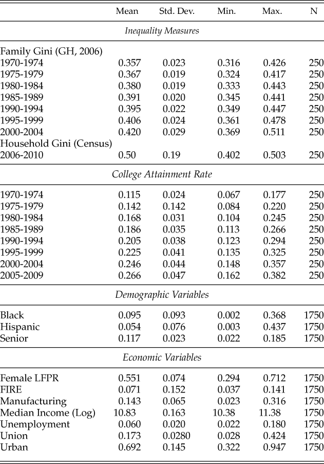
James Galbraith and Travis Hale estimate annual family income Gini coefficients for all fifty states over the period 1970–2004.Footnote 38 We use this data as our primary measure of income inequality in the analysis below. The independent variable of interest is the college attainment rate (college). State-level attainment data are from the 1970–2000 decennial Censuses of the Population and 2006–2010 American Community Surveys. Missing years are interpolated using the compound rate of growth between observable periods. In addition, we control for a number of additional economic and demographic variables that have been associated with income inequality in the literature. This includes the female labor force participation (female LFPR) and unemployment rates, natural log of median income (median income), percentages of the population that are African American (black), Hispanic (Hisp) and senior citizens (senior), the share of persons employed in the manufacturing and finance, insurance and real estate (FIRE) sectors, union density (union), and urbanization rate (urban). Details about these data and sources are given in the Appendix. Descriptive statistics for all of the state-level data are given in Table 1.
Summary Statistics
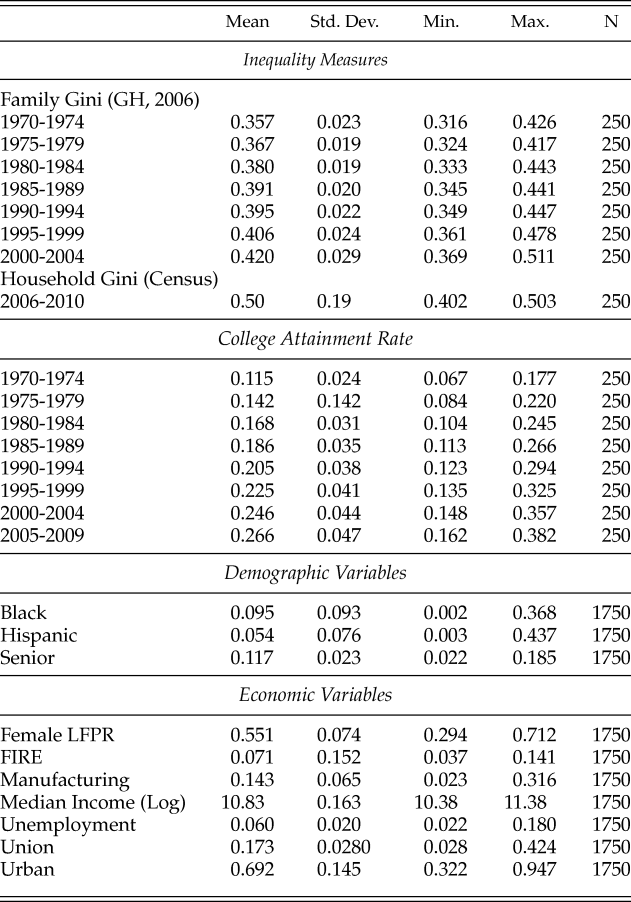
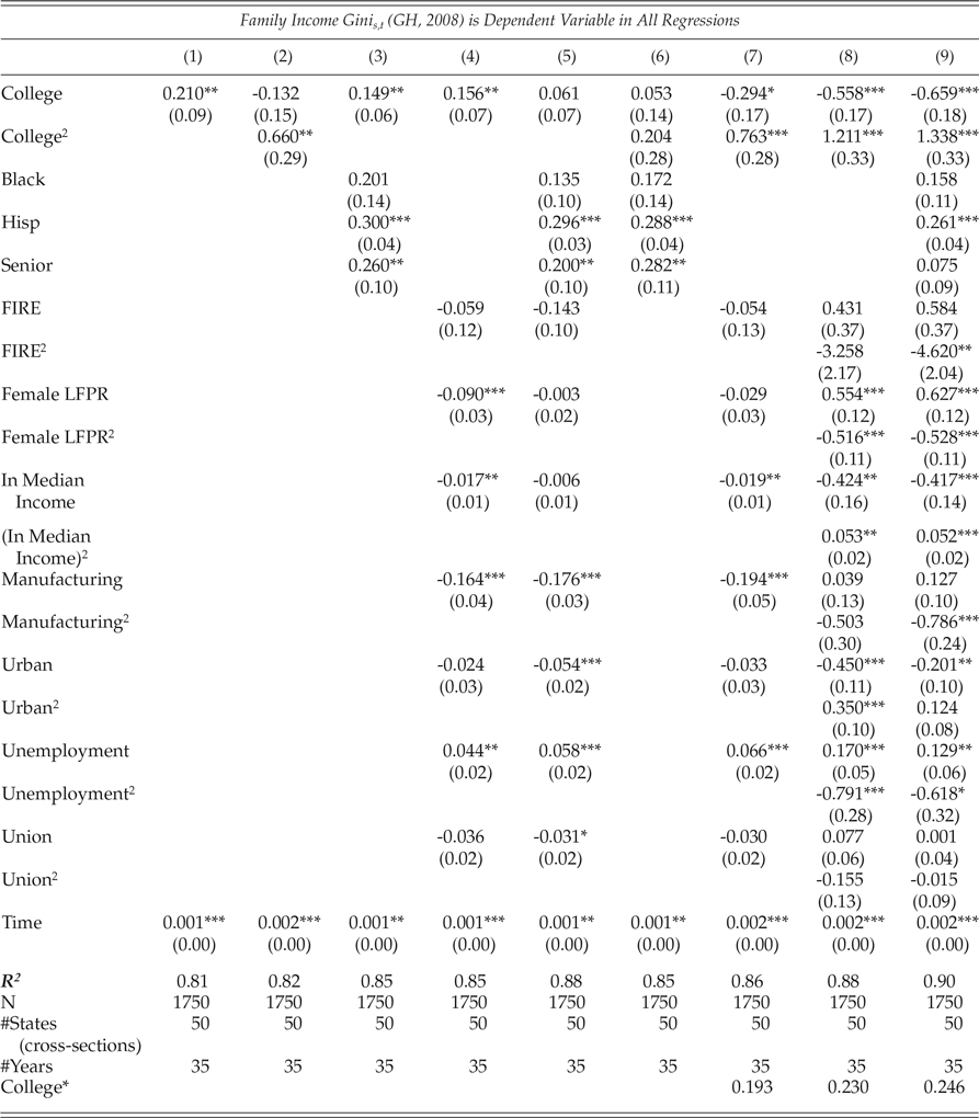
Table 2 reports the estimates using the entire panel of data. Column 1 includes college and the deterministic time trend (time), both of which are positive and statistically significant at 5 percent or better. Column 2 adds the college squared term, allowing for a nonlinear relationship. The linear and squared college terms have negative and positive coefficients, respectfully, forming a U-shaped inequality-attainment curve, although only the squared term is statistically significant.Footnote 39 Column 3 adds a set of three demographic variables (black, Hisp and senior) to the equation from column 1. Each has a positive sign but only the latter two are statistically significant. The linear college term remains positive and significant, although the magnitude of the partial effect is reduced relative to column 1. Column 4 adds a set of economic variables (FIRE, female LFPR, median income, manufacturing, urban, unemployment and union) to column 1 and the linear college term remains significant. Column 5 includes both the demographic and economic variables. The partial effect of college on inequality becomes insignificant in this specification.
Fixed-Effects Regression Results I
Clustered standard errors in parenthesis. Partial Effects assumed to be time invariant.
* p < 0.10,** p < 0.05,*** p < .01.
Columns 6–9 return to the nonlinear college-inequality specification from column 2. Column 6 includes the set of demographic variables. The estimates for the demographic variables are similar to those in column 3, but both college terms are positive and neither is significant. Column 7 adds the set of economic variables to the quadratic specification. The partial effects of the economic variables are qualitatively similar to those from column 4. Both the linear and squared college terms are significant at 10 percent or better in this specification, with the former negative and the latter positive, indicating a U-shaped inequality-attainment curve. Column 8 adds squared terms for each of the economic variables to account for potential nonlinear effects of these variables. The college and college square terms are both significant at one percent in this specification and maintain the U-shaped relationship. Column 9 adds the set of demographic variables to column 8. The college-inequality curve holds, as both college terms are significant at one percent.
The regressions from Table 2 explain 81 to 90 percent of the within-state variation in income inequality, depending on the specification, with column 9 having the highest R 2 value. Columns 7, 8, and 9 provide statistical evidence that there is a U-shaped relationship between college attainment and income inequality. This suggests that increases in college attainment from an initially low level act to reduce income inequality, but there are diminishing social returns such that there is an inequality-minimizing attainment rate, above which additional increases act to increase inequality. Using the partial effects from columns 7–9, we estimated the college attainment rate at which the partial effect of college attainment on inequality changes from negative to positive. We refer to this as the inequality-minimizing attainment rate and denote it as college* in the results. College* ranges from 0.193 to 0.246 in columns 7–9, suggesting that the current national college attainment rate of 30 percent is to the right of the inequality-minimizing curve such that additional increases in attainment are associated with more income inequality.
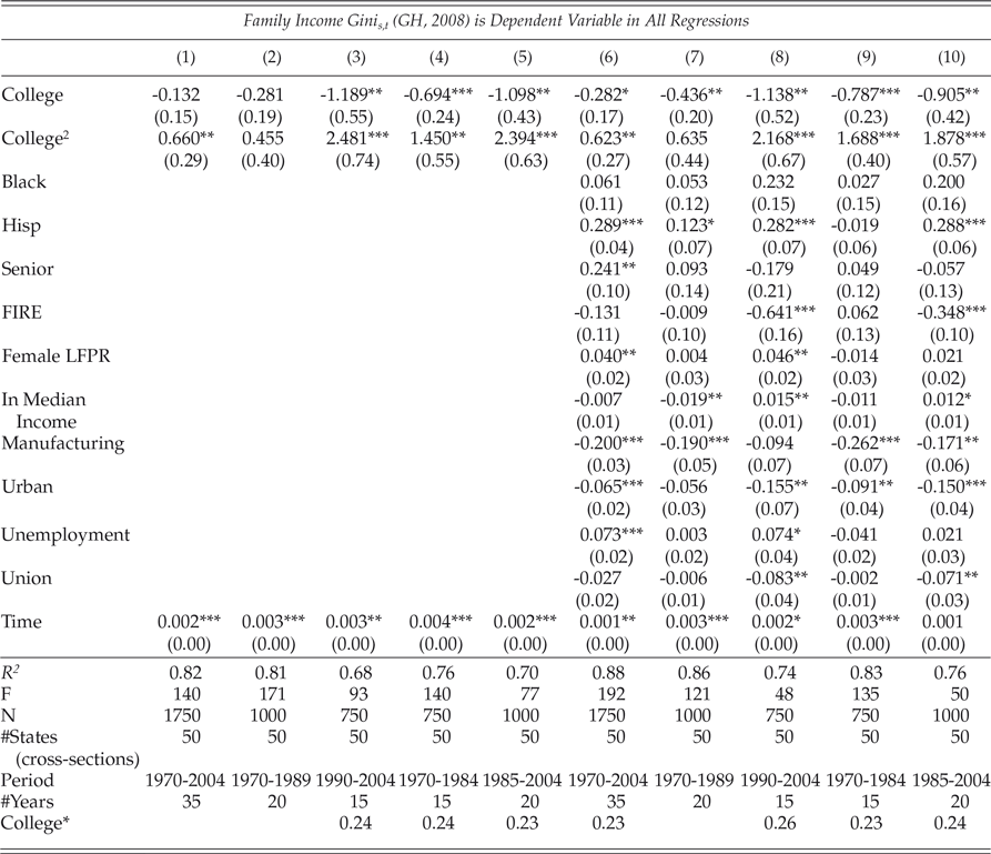
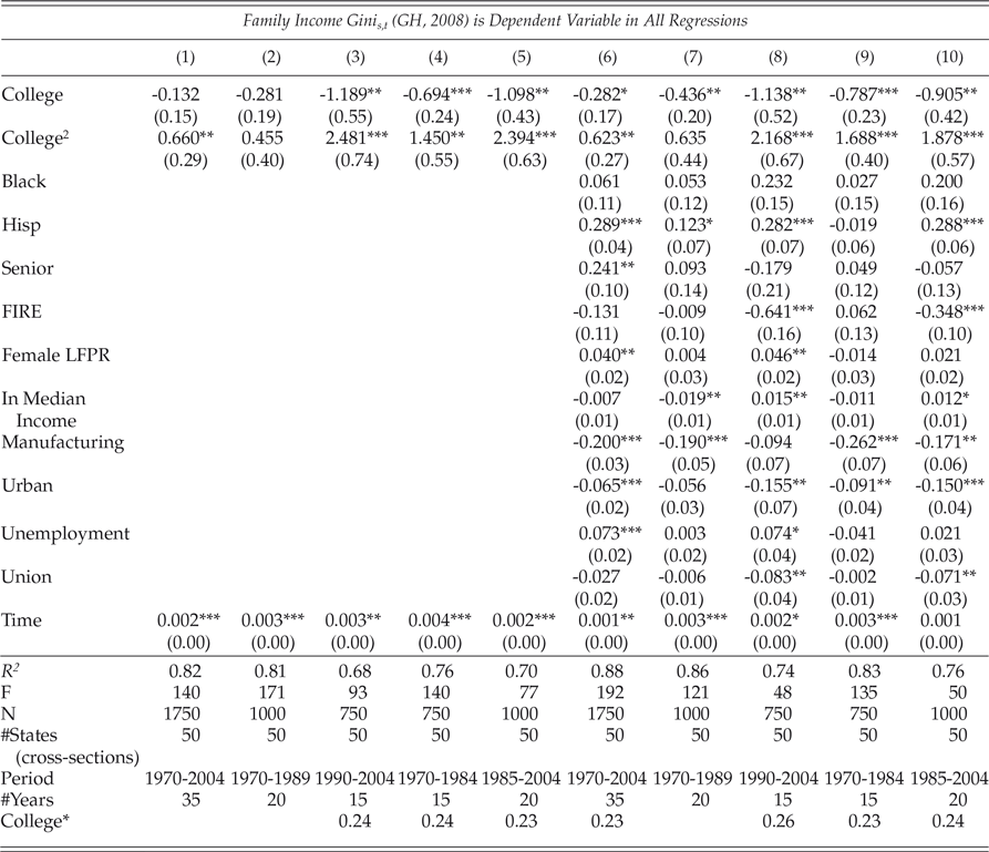
We further examine the college-inequality curve in Table 3 by examining subsets of the period. Columns 1–5 only include the linear and squared college terms. Column 1 reproduces the estimates from column 2 of Table 2, which utilized the entire 1970–2004 time period. Columns 2 and 3 repeat this specification but are restricted to the 1970–1989 and 1990–2004 periods, respectively. The U-shaped curve is present in both regressions, but the college terms are only significant (at 5 percent or better) in column 3. Columns 4 and 5 repeat this specification but are restricted to the periods 1970–1984 and 1985–2004, respectively. In both columns 4 and 5, the linear and squared college terms are significant (at 5 percent or better), with the former negative and the latter positive.
Fixed-Effects Regression Results II
Clustered standard errors in parenthesis. Partial Effects assumed to be time invariant.
College* is the estimated inflection point at which additional increases in college attainment exert a positive effect on income inequality.
* p < 0.10,** p < 0.05,*** p < .01.
Columns 6–10 add additional demographic and economic control variables. Column 6 serves as the baseline, as it includes all observations spanning the 1970–2004 time period. Columns 7 and 8 repeat the baseline for the sub-periods 1970–1989 and 1990–2004, respectively. As was the case in columns 2 and 3, both college terms are significant only in the latter time period, although the linear term is negative and significant in column 7. Columns 9 and 10 repeat the baseline for the sub-periods 1970–1984 and 1985–2004, respectively. Similar to columns 4 and 5, both college terms are significant at 5 percent or better for each period.
The results from Table 3 provide additional evidence of the existence of an inequality-minimizing college attainment rate.Footnote 40 These results suggest however that the inequality-minimizing attainment rate remains constant for relatively long periods of time — up to thirty-five years. Figure 4 plots the family income Gini against the college attainment rate for five-year intervals beginning in 1970. Casual observation of these graphs suggests that the relationship between the two variables has changed over time and that the inequality-minimizing attainment rate may have increased over time. This seems practical given that the structure of the economy changes over time and changes in the education level of the workforce influence the composition of workers and their wages, as suggested by economic theory.
Family Income Gini vs. College Attainment Rate, 1970–2004.
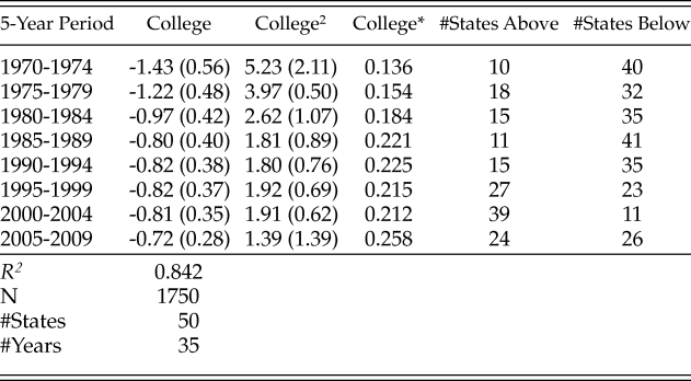
Next we estimate the inequality-minimizing college attainment rate by five-year period. We do so by interacting the linear and quadratic college terms with a series of seven dummy variables equal to one if the observation occurs during the five-year interval dj,j = [1970–1974, 1975–1979, ... , 2000–2004], and zero otherwise. Equation 2 describes the regression to be estimated. Table 4 gives the results, including the number of states below and above college* for each period. It also includes the results from a separate regression using annual state household income Gini measures from the American Community Survey as the dependent variable over the period 2006–2010 in column 8. All of the college terms are significant at 5 percent or better and the equation explains about 84 percent of the within-state variation of income inequality.
 $$Gini_{s,t} = \mathop \sum \limits_{j = 1}^7 \left[ {\beta _j \left( {College_{s,t} \times dj} \right) + \mu _j \left( {College_{s,t}^2 \times dj} \right)} \right] + \gamma t + c_s + u_{s,t} $$
Inequality-Minimizing Attainment Rate
Clustered standard errors in parenthesis.
College* is the estimated inequality-minimizing attainment rate. The 2005-2009 period uses household income Gini coefficients from the American Community Survey as dependent variables. The remaining results were derived using family income Gini coefficiens (GH, 2008) as the dependent variable. Deterministic time trend was included in both regressions - results omitted.
* p < 0.10,** p < 0.05,*** p < .01.
Prior to the latter part of the 1990s, most states had an average attainment rate below the inequality-minimizing point, suggesting that the states could have experienced additional increases in attainment without exacerbating inequality (indeed, moderately reducing it). College* was 0.136 during the first half of the 1970s and only ten states had an attainment rate above 13.6 percent.Footnote 41 By the latter part of the decade, the inequality-minimizing rate increased to 0.154 and another eight states moved to the right of college*. Footnote 42 The inflection point increased to 0.184 during the first part of the 1980s, although three fewer states achieved an attainment rate above college*.Footnote 43 The inequality-minimizing rate grew to 0.22 in the latter part of the 1980s and first half of the 1990s before rescinding slightly to 0.21 in the late 1990s and first five years of the new millennium. College attainment continued to grow and by the latter part of the 1990s, the majority of states surpassed the estimated inflection point. In the early 2000s, thirty-nine states had achieved an attainment rate above college*, suggesting that the inequality-reducing dimension of higher education had largely been exceeded and diminishing returns set in. The inequality-minimizing rate for the period 2005–2009 pertains to household income inequality as opposed to family income inequality. Although measures of the former typically suggest greater inequality than the latter, the estimates nonetheless suggest that approximately half of the states exceeded college* during the period.Footnote 44
IV. Policy Implications
Public policy designed to increase college enrollment and completion may be done with good intentions, but it can lead to unintended consequences. As discussed above, one consequence has been a watering down of the curriculum to accommodate less academically prepared students. This has coincided with grade inflation. These trends have reduced the potential of human capital gains of a college education as well as distorted the signal that a college credential sends to employers about the ability and work effort of a prospective employee.
The upward shift in the supply of college-credentialed workers has exceeded the increase in demand from the labor force. Rather than drive down the wage level of college workers and raise the wages of the non-college-educated workers, working to decrease inequality as a static analysis would predict, this largely government-induced disequilibrium has instead resulted in the displacement of non-college-educated workers with college-credentialed workers. Given the choice between hiring college and high-school educated workers to fill relatively low paying and low skill positions, employers are increasingly hiring the former as evidenced by rising underemployment of college graduates. As a result, the latter group has a harder time finding employment in sectors that have historically been open to them. Thus, policies designed to induce greater college attendance as a means to open the doors of opportunity and promote more equality may result in the opposite effect.
Another factor contributing to fundamental changes in the equality-higher education attainment relationship over time is the rising cost of college. Over the past thirty years or so, tuition fees have risen at roughly double the rate of inflation. More importantly, the growth in tuition fees greatly exceeds the growth in median family income. To be sure, net (after tuition discounts) fees have risen somewhat less dramatically, but there is evidence that students applying for college are heavily influenced by “sticker” prices — undiscounted tuition fees, since the amount of scholarship aid is unknown at the time of original application.
Sensitivity to prices generally falls as income rises. In this context, the increase in tuition fees, even relative to income levels, has no doubt disproportionately led some lower income Americans to avoid college on the grounds that it is too expensive. Federal data painstakingly analyzed by Thomas Mortenson suggests that in 1970, about 12 percent of twenty-four-year olds with college degrees came from the bottom quartile of the income distribution, compared with a meaningfully smaller proportion (about 10 percent) in 2011.Footnote 45 Colleges are becoming far more unequal economically, the rhetoric of college presidents notwithstanding.
Space does not permit an elaborate analysis of the determinants of rising college costs. One very likely culprit, however, is the explosive growth in federal student assistance programs, a view commonly accredited to former Secretary of Education William Bennett who was the first to publicly express it in an editorial more than twenty-five years ago.Footnote 46 While there is definitely divided opinion on the veracity of the Bennett Hypothesis, the best recent studies we have seen are generally at least partially supportive of it.Footnote 47 No one questions that federal student aid increases the demand for higher education, and given restraints on educational supply (e.g., selective admissions, accrediting rules restraining new college entrants), on theoretical grounds the net effect of enhanced federal student financial aid is almost certainly an increase in prices (tuition fees) as well as enrollments. The federal government makes low cost loan money available to young persons, who feel they now can “afford” to go to college. The colleges, seeing this, raise their fees from what would otherwise be the case, pushing up prices. Since much of the lending is being done to middle class and even moderately affluent students and parents, the net effect to lower-income student enrollments may be that the government’s impact on pushing fees up may more than offset any positive impact of student financial aid to lower-income students. Thus, the federal student financial aid program’s explosive growth (5.4 percent real annual compound rate since 1971) may have had the unintended consequence of making higher education more a haven for the affluent, reducing intergenerational income mobility and actually increasing income inequality.Footnote 48
V. Conclusions
The analysis presented here indicates that the relationship between college attainment and income inequality probably has changed over time, which is plausible since changes in the structure and composition of the workforce exert an impact on the dynamic real economy. Theory and empirical evidence suggest that there may be a higher education Laffer Curve. Expanding college attainment may act to reduce income inequality to some extent, but there may exist a critical attainment rate beyond which additional growth in college attainment may exacerbate income inequality, particularly if the supply of college-educated workers grows faster than the demand. We estimated this critical point and find that prior to the mid-1980s, most states were able to sustain increases in college attainment without increasing inequality. Since then the attainment rate has soared nationally, influenced significantly by the vast expansion of federal student financial assistance, particularly the provision of government loans to middle- and high-income families. By the latter part of the 1990s, the majority of states achieved an attainment rate exceeding the critical point such that additional increases in college completion may be acting to exacerbate inequality.
Higher education is becoming more and more an oasis for higher- and middle-income kids. Whereas at one time a degree from, say, Slippery Rock State College was not vastly less impressive to employers than one from, say, Harvard, that is no longer the case. Relatively fewer lower-income students graduate, and they increasingly attend colleges perceived as qualitatively inferior. Egged on by propaganda from colleges, high-school guidance counselors, political leaders, and some foundations, students increasingly borrow large sums of money, and yet a large portion fail to graduate or, if they do, take low paying jobs previously staffed by noncollege graduates, contributing to rising student loan default rates. The less affluent students increasingly are finding college a bad deal — contributing to the probability that increased college attainment actually promotes greater income inequality.
While there are certainly many factors contributing to the rise of income inequality, the analysis presented here should at least cause us to pause and rethink the role of public policy designed to promote greater college attainment as a means to achieve greater equality. The decades-long expansion of federal subsidization of higher education enrollment could be triggering the opposite effect.
Appendix: Data Sources
In the statistical analyses, we control for a number of other demographic and economic variables that may influence the distribution of income. These data and their sources are described in this appendix. Summary statistics for all of the data are presented in Table 1 above.
The economic variables include the female labor force participation rate (LFPR), the shares of employment in the finance, insurance and real estate (FIRE) and manufacturing industries, real log median income, the annual average state unemployment rate, the urbanization rate and union density.
The female LFPR is defined as the share of the civilian, noninstitutional females above sixteen years of age in the labor force in each state. The data come from two sources. The primary source is the U.S. Bureau of Labor Statistics’ (BLS) Current Population Survey, which provides the annual average of monthly labor force participation rates over the period 1976–2010, although several years (1977, 1980, 1981, 1989, 1997, 2006) were not available.Footnote 49 Next, the 1970 Census of the Population provides state-level female LFPRs. State-level female LFPRs were not available for the 1971–1975 period in addition to the individual years indicated above. National female LFPRs were, however, available annually for the entire 1970–2010 period.Footnote 50
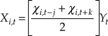
Data for the missing years was interpolated using equation 3, where X i,t is the interpolated female LFPR for state i in year
t, Y t is the national LFPR in year t,  $\chi _{i,t} = X_{i,t} /Y_{i,t} $ is the ratio of the LFPR in state i in year
t to the national LFPR in year t, and
j and k are the number of years since the
last and next, respectively, actual state-level female LFPRs are available.Footnote 51
 $$X_{i,t} = \left[ {{{\chi _{i,t - j} + \chi _{i,t + k} } \over 2}} \right]Y_t $$
The FIRE and manufacturing shares of employment ratios are computed using annual state-level data from the Bureau of Economic Analysis, with both having total employment as the denominator. Due to the change in industry classification codes in 1997, industry employment data are not directly comparable over the entire period of study, although the total employment figures are identical under both systems. U.S. Federal statistical agencies adopted the North American Industry Classification System (NAICS) in 1997, replacing the Standard Industrial Classification (SIC) system that had been in place since 1937. The BEA provides SIC data from 1969–2001, and NAICS data from 1990–2010. The total employment data for the two classifications matches for the overlapping years, but the FIRE and manufacturing employment data differ. Because our analysis covers the period 1970–2004, we need to make an adjustment in order to make the data comparable over the period of study. We do so using data from the period 1990–2001 since it is available for both systems.
The SIC FIRE employment data are given under the broad industry heading “Finance, Insurance and Real Estate.” The corresponding NAICS figure used in the present analysis is the sum of the “Finance and Insurance” and “Real Estate and Leasing” industry categories in an effort to match the corresponding sectors encompassing the respective classification systems. Both the SIC and NAICS systems report manufacturing employment numbers, but the two figures differ due to the reclassification of sectors.
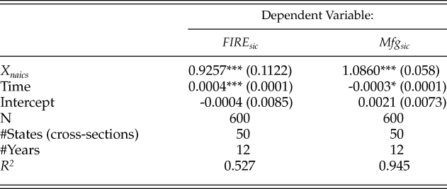
The correlation between the FIRE employment shares under the two classification systems for the overlapping years is 0.956 for the period 1990–2001, with the correlation coefficients for the individual years ranging from 0.921 in 1994 to 0.985 in 2001.Footnote 52 The correlation between the manufacturing employment shares under the two classifications for the period 1990–2001 is 0.990, with the correlation for single years ranging from 0.984 in 1991 to 0.994 in 1997. Thus, the ratios for both variables between the two datasets are highly correlated. As such, we employ a fixed effects regression model to predict the SIC employment ratios for post-2001 years using the NAICS employment ratios and deterministic trend as a control variable to account for employment trends. The model is given by equation 4, where X sic and X naics are the employment ratios for the SIC and NAICS systems, respectively, and t is deterministic trend such that t=1 represents 1990. The results from the regression are reported in Table 5.
 $$X_{sic_{s,t} } = \beta X_{naics_{s,t} } + \nu t + c_s + e_{s,t} $$
Predict SIC Ratios
Nominal state median household income data for 1975 and the period 1984–2010 are from U.S. Census Bureau's Current Population Survey, and are augmented by decennial state median income measures for 1969 and 1979. Figures for the missing years spanning 1970–1974, 1976–1978 and 1980–1983 were interpolated using the average annual compound growth rate between observation years to estimate the missing measures. Nominal median income figures were adjusted to constant 2011 dollars using the CPI-U. The natural log of the real median income figure is used. Median income is included as a measure of the level of income in a state.
Annual state unemployment rate data spanning the period 1970–2010 were collected from the Statistical Abstract of the United States.Footnote 53 Urban population data are from the 1969–2009 decennial Censuses of the Population. We use the annual compound growth rates between Censuses to linearly interpolate the between-Census figures.Footnote 54 Union density data are from Hirsch, MacPherson, and Vroman (2001), who estimate the share of non-agricultural unionized labor annually by state.Footnote 55
We include age, race, and ethnic characteristics of the population to control for state demographic trends. Age data are reported annually by the Population Distribution Branch of the U.S. Census Bureau. We use the share of the population above age sixty-five (senior) as a control variable. We also control for racial and ethnic characteristics of the population by including the percent of the population that is black and Hispanic. Data for these two variables are from the decennial Censuses, with between Census observations interpolated using the annual compound state growth rate for each variable.