1 Introduction
The determination of laminar to turbulent transition in supersonic flows is crucial for the aero- and aerothermodynamic design of re-entry vehicles (Pate Reference Pate1977; Khan & Reshotko Reference Khan, Reshotko, Eppler and Fasel1980). The predicted heat flux, which can be higher by more than just one order of magnitude in turbulent compared to laminar boundary layers, is an essential design parameter (Wurster Reference Wurster1981; Lin, Grabowsky & Yelmgren Reference Lin, Grabowsky and Yelmgren1984; Bouslog et al. Reference Bouslog, An, Hartmann and Derry1991). Since experimental wind tunnel data of boundary layer transition are known to be affected by tunnel noise (Reshotko Reference Reshotko1994; Fedorov Reference Fedorov2003, Reference Fedorov2011; Ma & Zhong Reference Ma and Zhong2003a ,Reference Ma and Zhong b , Reference Ma and Zhong2005; Zhong & Wang Reference Zhong and Wang2012; Fedorov et al. Reference Fedorov, Ryzhov, Soudakov and Utyuzhnikov2013), i.e. it strongly influences the region of transition (Schneider Reference Schneider2001, Reference Schneider2008a ,Reference Schneider b ), it is necessary to know the noise inherent to the test facility to properly evaluate and interpret the experimental results. Furthermore, knowledge of wind tunnel noise is essential to numerically compute the receptivity phenomenon for the specific noise of the wind tunnel and, thus, to improve the comparability between experiment and simulation.
The noise level of supersonic wind tunnels is mostly described by normalised root-mean-square (nRMS) pressure fluctuations measured by blunt axisymmetric transducers facing the flow. The supersonic nature of the flow leads to a detached shock wave upstream of the transducer increasing the entropy and reducing the total pressure of the flow. Therefore, a blunt stagnation point probe (SPP) measures the postshock total pressure and its fluctuations caused by postshock acoustic waves. Since free stream acoustic waves undergo modulation during the transmission through the shock wave, the measured disturbances do not represent the free stream and require a calibration, i.e. a transfer function relating free stream and postshock disturbances. Note that also entropy and vorticity disturbances in the free stream cause postshock acoustic waves (McKenzie & Westphal Reference McKenzie and Westphal1968; Chaudhry & Candler Reference Chaudhry and Candler2017). The modal decomposition of the measured data is a major goal of ongoing research and strongly related to this work (Schilden & Schröder Reference Schilden and Schröder2017). Nevertheless in this study, the focus lies on transfer functions relating inclined slow acoustic waves and postshock total pressure fluctuations measured by SPPs since this type of disturbance is radiated by the turbulent nozzle boundary layer in supersonic wind tunnels and constitutes a great portion of the measured tunnel noise (Laufer Reference Laufer1961; Duan, Choudhari & Wu Reference Duan, Choudhari and Wu2014). If these acoustic disturbances are orders of magnitude higher than the entropy or vorticity disturbances, the transfer functions can be directly applied to measured data. If the wind tunnel noise composition is more homogeneous, the transfer functions are plugged into modal decomposition methods to decompose measured data into the disturbance modes (Kovasznay Reference Kovasznay1953; Logan Reference Logan1988; Schilden & Schröder Reference Schilden and Schröder2017). Either way, the calibration of SPPs by adequate transfer functions is crucial to determine tunnel noise. In the remaining part of this section, investigations considering noise radiated by turbulent boundary layers will be revisited and approaches and challenges to derive transfer functions between radiated noise and SPP measurements are elaborated.
The determination of acoustic waves radiated by supersonic boundary layers goes back to Laufer (Reference Laufer1961). Laufer performed hot-wire measurements in supersonic wind tunnel flows ranging from Mach numbers of
 $1.6$
to
 $5$
. He found the correlation between mass-flow and total temperature fluctuations to be approximately
 $-1$
. By investigating the eigenfunctions of the free stream disturbance modes regarding the corresponding correlation, he could relate the observed disturbances to the slow acoustic wave. Furthermore, he was able to determine the inclination of the radiated waves by exploiting the dispersion relation of acoustic waves and taking into account that hot-wires are only sensitive to the velocity disturbances in the mean flow direction. The inclination differs from the Mach wave inclination and can be related to a source velocity denoting the velocity of effective sound sources in the turbulent boundary layer. More details about his analysis and results are given in § 2.1.
Recently, Duan et al. (Reference Duan, Choudhari and Wu2014) numerically investigated the noise radiated by turbulent supersonic boundary layers (Zhang & Duan Reference Zhang and Duan2015; Huang et al.
Reference Huang, Zhang, Duan and Choudhari2017; Duan et al.
Reference Duan, Choudhari, Chou, Muñoz, Ali, Radespiel, Schilden, Schröder, Marineau and Casper2018). Space–time correlations of pressure fluctuations in the free stream were used to extract the dominant inclination of the radiated acoustic field and the corresponding source velocities. In comparison with the source velocity computed by Laufer (Reference Laufer1964), the agreement at Mach
 $2.5$
is excellent and the numerical result at Mach
 $6$
corroborates the linear relation of free stream Mach number and source velocity found by Laufer (Duan & Choudhari Reference Duan and Choudhari2013). Furthermore, spectral analysis and comparisons were conducted. The slow acoustic waves radiated by a turbulent boundary layer cover a wide range of frequency and amplitude, whereas the inclination shows a distinct Mach number dependence.
To compute the transfer function between the radiated acoustic waves and postshock pressure fluctuations measured by SPPs, Stainback & Wagner (Reference Stainback and Wagner1972) proposed a reduced-order method employing the Rayleigh Pitot-tube formula for high Mach numbers. Assuming quasi-steady changes of the flow, a low frequency limit for inclined slow acoustic waves was derived. Unfortunately, Stainback & Wagner overlooked a sign error and it will be shown in § 2.3 that the derived relation underestimates free stream acoustic waves. In a similar correct manner, Chaudhry & Candler (Reference Chaudhry and Candler2017) derived low frequency limits of non-inclined acoustic and entropy waves for SPPs by taking into account the full Rayleigh Pitot-tube formula. Naturally, reduced-order low frequency limits do not account for unsteady effects as, e.g. resonance. Furthermore, also the wave modulation occurring at higher wavenumbers due to the interaction of shock waves and slow acoustic waves is neglected (McKenzie & Westphal Reference McKenzie and Westphal1968). These drawbacks can be eliminated by direct numerical simulations (DNS).
Numerical simulations of non-inclined acoustic and entropy waves incident to a blunt body in supersonic flow were performed by Chaudhry & Candler (Reference Chaudhry and Candler2017) and later by Schilden & Schröder (Reference Schilden and Schröder2017). For any incident disturbance type, at certain frequencies oscillating acoustic waves in the subsonic region between shock wave and SPP lead to significant positive interference. The resonant behaviour of the transfer function is dictated by the duration of an acoustic wave travelling downstream from the shock wave to the probe, being reflected and propagating upstream to the shock wave. Using this time scale, the shock standoff frequency or Strouhal number can be determined. At integer multiples
 $n$
of the shock standoff Strouhal number destructive interference occurs whereas constructive interference arises for
 $n-0.5$
times the standoff Strouhal number. The offset of
 $0.5$
follows from an additional phase shift of
 $\unicode[STIX]{x03C0}$
during the reflection at the shock wave. The finding of significant resonance contradicts Morkovin’s (Reference Morkovin1960) hypothesis of intense damping during the reflection at the shock wave and rather scattered than focused acoustic waves downstream of the shock wave, but Chaudhry & Candler postulate a focusing effect due to the inward refraction of the postshock acoustic waves to strengthen the hitherto underrated interference. The positive interference was also found experimentally by Ali et al. (Reference Ali, Zárate Cárdenas, Radespiel, Schilden and Schröder2018). The demand of the transfer function for the ongoing research regarding the determination of tunnel noise, the recent numerical results revealing the shortcomings of reduced-order models like low frequency limits (Chaudhry & Candler Reference Chaudhry and Candler2017) and the popular disputable relation by Stainback & Wagner (Reference Stainback and Wagner1972) serve as motivation to expand the preceding numerical investigations of Schilden & Schröder (Reference Schilden and Schröder2017) to the numerical simulation of the interaction of inclined slow acoustic waves and SPPs.
The flow of the preceding numerical investigations was axisymmetric and could be computed at moderate computational costs. Investigations of the perception of inclined acoustic waves by SPPs are much more costly. The flow is three-dimensional and although symmetry can be exploited, the computational core hours rise by orders of magnitude depending on the degrees of freedom required by the numerical method to resolve the circumference. To circumvent this cost increase, a new axisymmetric boundary condition is proposed reducing the problem, i.e. the determination of transfer functions between inclined free stream acoustic waves and fluctuations measured by SPPs, to two dimensions while accounting for inclination related unsteady effects when evaluated in axisymmetric DNS. It will be shown in § 3 that the transfer functions at the stagnation point based on this axisymmetric concept are the exact transfer functions of the three-dimensional problem if linearity is ensured. Furthermore, exact circumferential averages can be attained within this concept.
The paper is organised as follows. In § 2, theoretical considerations on inclined slow acoustic waves incident to SPPs are discussed to characterise the interaction. Subsequently, the new axisymmetric boundary condition is presented and the underlying equations are derived in § 3. Then, the SPP of this investigation, the computational set-up and the flow condition are presented in § 4. In § 5, the results of the investigation are discussed. Finally, the essential findings are summarised. Scientists seeking practical information are referred to figures 8–10 and their discussion in §§ 5.2.1 and 5.2.2.
2 Inclined acoustic waves incident to an SPP
The propagation of low amplitude acoustic waves is accurately described by the linearised Euler equations. They are derived from the Navier–Stokes equations of a compressible fluid by neglecting friction and thermal conduction and by splitting the flow variables into mean and fluctuating parts. Higher-order terms are neglected to yield a linear system of equations. For uniform mean flow, e.g. free stream, and isentropic changes of state, the equations can be reduced to a single linear differential equation for pressure fluctuations
 $p^{\prime }$
featuring advection and wave propagation of the pressure field. For an ideal gas, the equation reads
 $$\begin{eqnarray}\left[\left(\frac{\unicode[STIX]{x2202}}{\unicode[STIX]{x2202}t}+\boldsymbol{u}_{\infty }\boldsymbol{\cdot }\unicode[STIX]{x1D735}\right)^{2}-a_{\infty }^{2}\unicode[STIX]{x1D6E5}\right]p^{\prime }=0.\end{eqnarray}$$
The quantity
 $\boldsymbol{u}_{\infty }$
denotes the constant unperturbed velocity and
 $a_{\infty }$
the speed of sound in the free stream. Plane acoustic waves radiated by a turbulent boundary layer propagate according to (2.1). They are described by a wave vector
 $\boldsymbol{k}$
and an angular frequency
 $\unicode[STIX]{x1D714}$
via
 $$\begin{eqnarray}p^{\prime }\propto \text{e}^{\text{i}(\boldsymbol{k}\boldsymbol{\cdot }x-\unicode[STIX]{x1D714}t)}.\end{eqnarray}$$
Inserting (2.2) into (2.1), the dispersion relation for plane acoustic waves reads
 $$\begin{eqnarray}(\boldsymbol{u}_{\infty }\boldsymbol{\cdot }\boldsymbol{k}-\unicode[STIX]{x1D714})^{2}=a_{\infty }^{2}\boldsymbol{k}\boldsymbol{\cdot }\boldsymbol{k}.\end{eqnarray}$$
Using
 $\unicode[STIX]{x1D719}$
as the inclination angle between wave vector and free stream velocity
 $u_{\infty }=|\boldsymbol{u}_{\infty }|$
, the two-dimensional wave vector
 $$\begin{eqnarray}\boldsymbol{k}=\frac{\unicode[STIX]{x1D714}}{u_{\infty }\cos (\unicode[STIX]{x1D719})\pm a_{\infty }}\left(\begin{array}{@{}c@{}}\cos (\unicode[STIX]{x1D719})\\ \sin (\unicode[STIX]{x1D719})\end{array}\right)\end{eqnarray}$$
can be determined. The positive sign denotes fast acoustic waves and the negative sign represents slow acoustic waves. The angular frequency
 $\unicode[STIX]{x1D714}$
can be expressed as Strouhal number
 $$\begin{eqnarray}Sr=\frac{\unicode[STIX]{x1D714}l_{ref}}{2\unicode[STIX]{x03C0}u_{\infty }}\end{eqnarray}$$
based on the reference length
 $l_{ref}$
and free stream velocity
 $u_{\infty }$
.
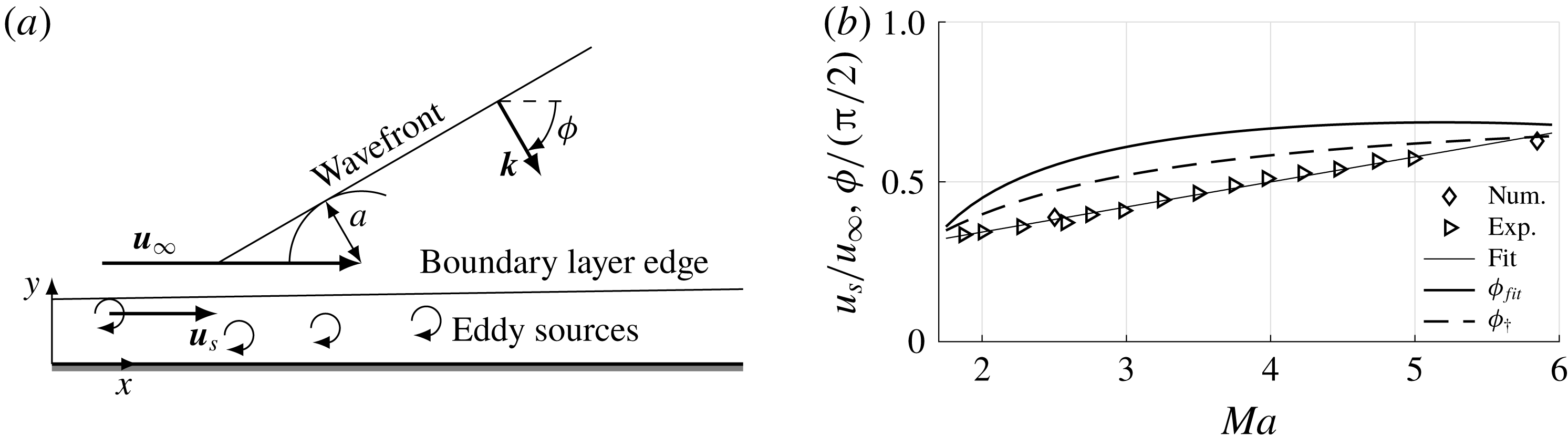
Plane acoustic waves radiated by eddy sources of a turbulent boundary layer: (a) the eddy sound sources propagate with
 $u_{s}$
in the boundary layer of a free stream velocity
 $u_{\infty }$
. Relative to the moving source, the radiated wave is a Mach wave; (b) non-dimensional source velocity
 $u_{s}/u_{\infty }$
and radiation angle
 $\unicode[STIX]{x1D719}_{fit}$
obtained by a linear fit of the data ‘Exp’ by Laufer (Reference Laufer1961) and ‘Num’ by Duan & Choudhari (Reference Duan and Choudhari2013), the critical angle of incidence
 $\unicode[STIX]{x1D719}_{\dagger }$
follows from (2.11).

Knowing the angle of inclination of the radiated waves, wave propagation and interaction theory is helpful to a priori analyse the impact of acoustic waves. The analysis can be conducted in two dimensions defined by the streamwise and normal coordinate
 $x$
and
 $y$
shown in figure 1(a). Although our model is two-dimensional, the
 $y$
-direction will be referred to as radial direction.
In the following, acoustic waves radiated by turbulent boundary layers are described and the subsequent interaction with the shock wave upstream of the probe in supersonic flow is revisited.
2.1 Inclined acoustic waves radiated by a turbulent boundary layer in supersonic flow
The incidence angle of radiated acoustic waves is linked to a source velocity
 $u_{s}$
denoting the velocity of eddies which act as acoustic sources in a turbulent boundary layer (Laufer Reference Laufer1961). Regarding the dispersion relation (2.3), the source velocity is the phase velocity of the radiated acoustic wave along the wall parallel coordinate
 $u_{s}=\unicode[STIX]{x1D714}/k_{x}$
. For slow acoustic waves, the dispersion relation requires source velocities in the interval
 $0\leqslant u_{s}\leqslant u_{\infty }-a$
. The radiation inclination can be linked to the source velocity
 $u_{s}$
by
 $$\begin{eqnarray}\cos (\unicode[STIX]{x1D719})=\left(1-\frac{u_{s}}{u_{\infty }}\right)^{-1}Ma^{-1},\end{eqnarray}$$
using the dispersion relation and the Mach number
 $Ma=u_{\infty }/a_{\infty }$
. Figure 1(a) shows this relation between
 $\unicode[STIX]{x1D719}$
and
 $u_{s}$
by a Mach wave construction illustration. Note that only the negative solution for
 $\unicode[STIX]{x1D719}$
of (2.6) describes a radiated wave since the wall normal
 $y$
component of the direction of energy propagation, i.e. the group velocity
 $\unicode[STIX]{x2202}\unicode[STIX]{x1D714}/\unicode[STIX]{x2202}\boldsymbol{k}$
, needs to be positive to be radiated from the boundary layer into the free stream. Then, the wave vector
 $\boldsymbol{k}$
of the radiated noise is directed towards the wall. The lower bound of the source velocity
 $u_{s}\rightarrow 0$
denotes the upper bound of
 $\unicode[STIX]{x1D719}=\cos ^{-1}(1/Ma)$
, i.e. a Mach wave, whereas the upper limit
 $u_{s}\rightarrow u_{\infty }-a$
causes a slow acoustic wave without inclination
 $\unicode[STIX]{x1D719}=0$
. An estimate of the Mach number dependence of the non-dimensional source velocity
 $u_{s}/u_{\infty }$
can be obtained by a linear fit of the experimental and numerical data by Laufer (Reference Laufer1961) and Duan & Choudhari (Reference Duan and Choudhari2013). In the range from
 $2\leqslant Ma\leqslant 6$
 $$\begin{eqnarray}\frac{u_{s}}{u_{\infty }}=0.0784\,Ma+0.1861\end{eqnarray}$$
can be used. The reference data, the fit (2.7) and the resulting inclination angle
 $\unicode[STIX]{x1D719}_{fit}$
based on (2.6) are shown in figure 1(b). Having defined the generated waves, their interaction with an SPP can be analysed.
2.2 Non-dimensional wavenumber map
To gain a simple and illustrative classification of the interaction of an SPP and inclined acoustic waves, besides the inclination angle
 $\unicode[STIX]{x1D719}$
and the Strouhal number
 $Sr$
, wavenumbers should be considered in the analysis. Assuming the bow shock upstream of the SPP to be a normal shock wave, the non-dimensional wave vector based on the diameter of the probe
 $\boldsymbol{k}_{D}=\boldsymbol{k}D/(2\unicode[STIX]{x03C0})$
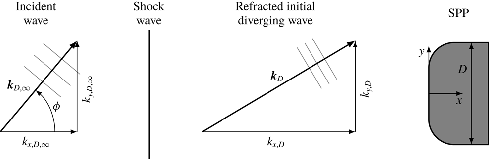
defining the transmitted acoustic wave immediately downstream of the shock wave can analytically be determined. Figure 2 illustrates the incident inclined acoustic wave in the free stream, the shock wave upstream of the SPP, the acoustic wave immediately downstream of the shock wave, i.e. the refracted initial diverging acoustic wave, and the SPP. In general, the term initial diverging is more appropriate than transmitted since the acoustic wave following from the initial interaction of the incident wave with the shock wave also occurs for incident entropy waves (Schilden & Schröder Reference Schilden and Schröder2017).
Illustration of the underlying model for § 2.2. The shock wave is approximated as a normal shock to analyse the interaction with the incident inclined acoustic wave. The radial wavenumber remains constant
 $k_{y,D}=k_{y,D,\infty }$
, whereas the axial wavenumber
 $k_{x,D,\infty }$
is altered to
 $k_{x,D}$
by refraction at the shock wave. Both wavenumbers are based on the diameter
 $D$
of the SPP. The grey lines indicate lines of constant phase being multiples of
 $2\unicode[STIX]{x03C0}$
.

The radial component of the non-dimensional wave vector, i.e. the radial wavenumber
 $k_{y,D}$
, defines the number of waves distributed over the radial extent of the probe. Note that the radial wavenumber is not altered by the interaction with the shock wave as indicated in figure 2 (McKenzie & Westphal Reference McKenzie and Westphal1968). From (2.4), the non-dimensional radial wavenumber can be derived
 $$\begin{eqnarray}k_{y,D}=\frac{Ma\,Sr\sin (\unicode[STIX]{x1D719})}{Ma\cos (\unicode[STIX]{x1D719})-1}.\end{eqnarray}$$
The reference length of the Strouhal number
 $Sr$
is the diameter of the probe.
Chaudhry & Candler (Reference Chaudhry and Candler2017) showed that the Strouhal number determines the resonance, i.e. constructive and destructive interference, of bidirectionally oscillating acoustic waves. For non-inclined incident plane waves the Strouhal number defines the phase difference
 $\unicode[STIX]{x0394}\unicode[STIX]{x1D711}$
between the initial diverging postshock acoustic wave and its shock reflected acoustic wave (Schilden & Schröder Reference Schilden and Schröder2017). This phase difference and the Strouhal number are linked via the axial wavenumbers of postshock slow (sa) and fast (fa) acoustic waves, i.e. body and shock reflected acoustic waves oscillating between shock wave (sw) and stagnation point (sp), by
 $$\begin{eqnarray}\unicode[STIX]{x0394}\unicode[STIX]{x1D711}=\int _{sp}^{sw}k_{x,sa}(x)\,\text{d}x+\int _{sw}^{sp}k_{x,fa}(x)\,\text{d}x+\arg (c_{I}).\end{eqnarray}$$
The term
 $\arg (c_{I})$
denotes an additional phase difference introduced by the transfer function
 $c_{I}$
by the reflection of acoustic waves incident to the shock wave from the downstream (Schilden & Schröder Reference Schilden and Schröder2017). The wavenumbers
 $k_{x,sa}$
and
 $k_{x,fa}$
in (2.9) also depend on the inclination of the acoustic waves since the free stream axial wavenumber of an acoustic wave is heavily modulated by refraction when it passes the shock wave. The refraction induced by the shock wave is defined by the change of velocity and speed of sound in the dispersion relation (2.3). The non-dimensional postshock axial wavenumber
 $k_{x,D}$
is derived by coupling the dispersion relations of the free stream and postshock acoustic waves for constant Strouhal numbers and radial wavenumbers as illustrated in figure 2. The relation reads
 $$\begin{eqnarray}k_{x,D}=\frac{Ma_{2}MaSr}{\unicode[STIX]{x1D705}(Ma_{2}^{2}-1)}+\sqrt{\left(\frac{MaSr}{\unicode[STIX]{x1D705}(Ma_{2}^{2}-1)}\right)^{2}+\frac{k_{y,D}^{2}}{Ma_{2}^{2}-1}},\end{eqnarray}$$
where
 $Ma_{2}$
is the Mach number downstream of a normal shock wave and
 $\unicode[STIX]{x1D705}=a_{2}/a_{\infty }$
denotes the ratio of postshock and free stream speed of sound.
A critical angle of incidence
 $\unicode[STIX]{x1D719}_{\dagger }$
is reached when the discriminant of (2.10) becomes zero (Robinet & Casalis Reference Robinet and Casalis2001). For angles
 $\unicode[STIX]{x1D719}>\unicode[STIX]{x1D719}_{\dagger }$
, the axial wavenumber is complex, the real part of
 $k_{x,D}$
remains constant, whereas the imaginary part grows further with increasing angle of incidence. The imaginary part of the axial wavenumber causes an axial attenuation of the transmitted wave. Such waves are therefore called attenuated waves or evanescent waves. Moore (Reference Moore1954) terms such waves pressure waves rather than acoustic waves, since they do not propagate at the speed of sound. A relation for the critical angle is derived from the discriminant and (2.10)
 $$\begin{eqnarray}\left.\begin{array}{@{}c@{}}\displaystyle \unicode[STIX]{x1D719}_{\dagger }=\cos ^{-1}\left(\frac{\unicode[STIX]{x1D6FD}}{\sqrt{1+(\unicode[STIX]{x1D6FD}Ma)^{2}}}\right)-\tan ^{-1}((\unicode[STIX]{x1D6FD}Ma)^{-1})\\ \displaystyle \unicode[STIX]{x1D6FD}=\left(\unicode[STIX]{x1D705}\sqrt{1-Ma_{2}^{2}}\right)^{-1}.\end{array}\right\}\end{eqnarray}$$
The Mach number dependence of the critical angle
 $\unicode[STIX]{x1D719}_{\dagger }$
is shown in figure 1(b). In the considered Mach number range,
 $\unicode[STIX]{x1D719}_{\dagger }$
is always smaller than the angle of the acoustic waves radiated by a turbulent boundary layer.
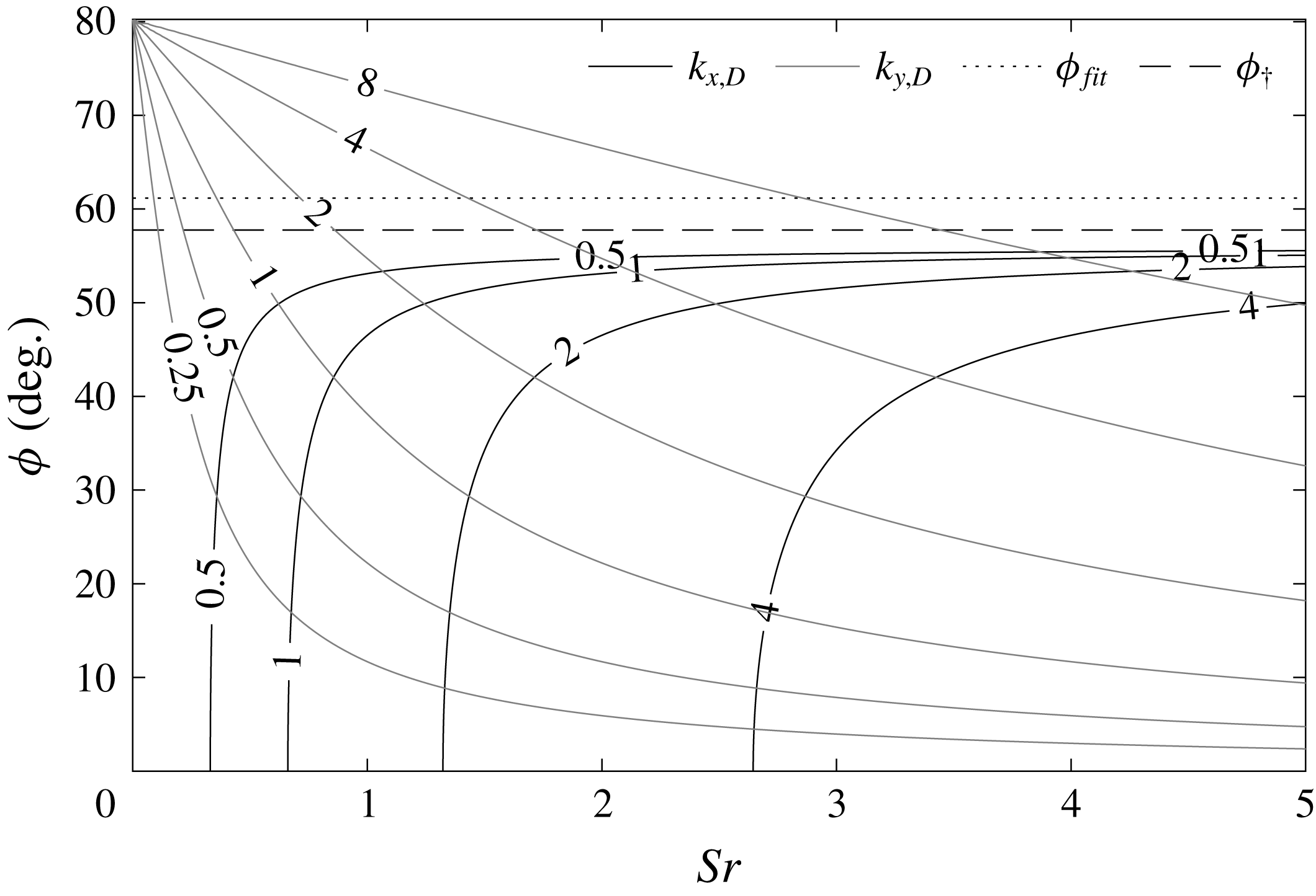
Using an additional set of parameters, i.e. the postshock wavenumbers (2.8) and (2.10), to describe the incident wave and the critical angle of interaction (2.11) to classify the type of interaction, the non-dimensional wavenumber map in figure 3 is generated for an SPP in
 $Ma=5.9$
flow. Grey lines denote constant radial wavenumbers and constant axial postshock wavenumbers are drawn in black. Isolines for axial wavenumbers at
 $\unicode[STIX]{x1D719}>\unicode[STIX]{x1D719}_{\dagger }$
are not shown. The critical incidence angle
 $\unicode[STIX]{x1D719}_{\dagger }$
is the dashed horizontal line. The fit for acoustic waves radiated by a turbulent boundary layer employing (2.7) is included as dotted line. In the following, the wavenumber map is discussed and implications to detect incident waves are made based on the presented theory.
Non-dimensional wavenumber map of a probe in Mach
 $5.9$
flow exposed to inclined slow acoustic waves. The black solid lines define constant axial wavenumbers
 $k_{x,D}$
for
 $\unicode[STIX]{x1D719}<\unicode[STIX]{x1D719}_{\dagger }$
. The grey lines denote constant radial wavenumbers
 $k_{y,D}$
. The dashed line is the critical angle of wave refraction
 $\unicode[STIX]{x1D719}_{\dagger }$
and the dotted line represents the estimate of radiated noise based on (2.7).

For low radial and axial wavenumbers, the probe perceives the disturbance as quasi-steady deviation from the free stream. In this regime, reduced-order methods like the low frequency limit accurately describe the transfer function. This regime is located on the left of figure 3 confined by either low axial or radial wavenumbers. An analytic expression of the low frequency limit will be given in § 2.3. A result for the validity range of the reduced-order method based on a critical deviation and parameters of the incident wave does not exist.
At zero inclination, resonance was found to be important. Let the axial wavenumber
 $k_{x,D,ac}$
be the postshock wavenumber at the shock standoff Strouhal number
 $Sr_{ac}$
. For
 $k_{x,D}=k_{x,D,ac}(n-0.5)$
,
 $n$
being a positive integer, constructive interference occurs and for
 $k_{x,D}=k_{x,D,ac}n$
postshock acoustic waves superpose destructively. The radial wavenumber is
 $k_{y,D}$
zero. Increasing the inclination angle from zero towards the dotted line in figure 3, i.e. the inclination of radiated waves, at constant Strouhal number, the radial wavenumber increases and the axial wavenumber decreases. At small inclination angles in the depicted
 $k_{x,D}$
range, the axial wavenumber is insensitive to the change of inclination. Significant changes in the resonant behaviour cannot be expected. This statement will be confirmed in § 5. From a certain angle on towards
 $\unicode[STIX]{x1D719}_{fit}$
, the lines of constant axial wavenumber rapidly turn to higher Strouhal numbers. For
 $k_{x,D}=0.5$
, high deviations from the Strouhal number at
 $\unicode[STIX]{x1D719}=0$
start to occur above
 $40^{\circ }$
. With increasing axial wavenumber, high deviations start to arise at lower inclination angles, e.g.
 $20^{\circ }$
for
 $k_{x,D}=4$
. Following the assumption that the resonant behaviour is determined by the axial wavenumber, changes of the type of interference might be suspected with increasing inclination angle, i.e. the resonant valleys and peaks are shifted to higher Strouhal numbers. On the other hand, the flow between shock and probe is neither uniform nor quiescent and the axial wavenumbers in (2.9) might not be well represented by (2.10), e.g. further refraction occurs during the reflection at the shock wave (Robinet & Casalis Reference Robinet and Casalis2001). Furthermore, the transfer function of the reflection of acoustic waves incident from downstream of the shock wave
 $c_{I}$
is important for the resonance behaviour. At zero inclination, the transfer function is real and negative thus introducing the phase shift of
 $\unicode[STIX]{x03C0}$
between incident and reflected wave in (2.9) (Chaudhry & Candler Reference Chaudhry and Candler2017). With increasing angle of incidence, the transfer function increases to values greater than zero before it decreases to negative values again which also alters the resonant behaviour (McKenzie & Westphal Reference McKenzie and Westphal1968; Robinet & Casalis Reference Robinet and Casalis2001). Altogether, even for this simple SPP–acoustic-wave interaction, the resonant behaviour for high inclination angles below the critical angle
 $\unicode[STIX]{x1D719}_{\dagger }$
is difficult to investigate and thus, will be analysed by DNS in § 5.2.3.
Acoustic waves radiated by turbulent boundary layers possess a high inclination. For
 $Ma=5.9$
, (2.7) results in
 $\unicode[STIX]{x1D719}_{fit}=61.16^{\circ }$
, i.e. it is higher than the critical angle
 $\unicode[STIX]{x1D719}_{\dagger }=57.76^{\circ }$
of the interaction of the normal shock with the inclined slow acoustic wave. At low Strouhal numbers, the low frequency limit holds but the radial wavenumber distribution along
 $\unicode[STIX]{x1D719}_{fit}$
increases rapidly with advancing Strouhal number. For non-inclined waves, resonance and the focusing effect lead to an amplification of incident waves at low Strouhal numbers
 ${<}Sr_{ac}$
. The higher
 $Sr$
, the more applicable the linear theory of interaction of acoustic waves with shock waves by McKenzie & Westphal (Reference McKenzie and Westphal1968), since the detached bow shock locally appears more straight in comparison to the wavelength of the incident wave. According to the linear theory, the interaction of the radiated waves at
 $\unicode[STIX]{x1D719}_{fit}$
with a normal shock wave generates attenuated waves downstream of the shock and therefore, low transfer functions can be expected. Furthermore, transfer functions of the linear theory considering the transmission of plane waves are independent of the Strouhal number. For postshock attenuated waves, the spatial decay of pressure fluctuations is prescribed by the imaginary part of the axial wavenumber, and thus a Strouhal number dependence at a fixed distance downstream of the shock wave occurs. On the other hand, the curved bow shock interacts with the incident waves at varying angles over the radial and circumferential extent before the wave ultimately reaches the probe. Again, various effects compete and impede a clear assessment of the Strouhal number effect at inclination angles of waves radiated by turbulent boundary layers. The transition between low and high Strouhal number effects for these waves is investigated by DNS in § 5.2.1.
Furthermore, with increasing Strouhal number at radiation inclination or in general with increasing inclination angle at constant Strouhal number, growing radial wavenumbers lead to averaging effects since transducers have a finite size. The fluctuations caused by the inclined wave possess phase differences on the surface resulting in cancellation. The larger the wavenumber on the surface or the larger the transducer area, the larger the phase differences become and the effect of averaging increases. This effect will also be quantified in § 5. Next, the low frequency limit is derived before the DNS are presented.
2.3 Low frequency limit for inclined slow acoustic waves
The transfer function
 $r_{p}$
is defined as the non-dimensional ratio of stagnation point pressure fluctuation
 $p_{t}^{\prime }$
and free stream density fluctuations
 $\unicode[STIX]{x1D70C}_{\infty }^{\prime }$
 $$\begin{eqnarray}r_{p}=\frac{p_{t}^{\prime }}{p_{t}}\frac{\unicode[STIX]{x1D70C}_{\infty }}{\unicode[STIX]{x1D70C}_{\infty }^{\prime }}.\end{eqnarray}$$
Assuming sinusoidal fluctuations, the primed values are represented by complex numbers and the absolute value
 $|r_{p}|$
is the ratio of fluctuation amplitudes. The density based scaling yields a common formulation for incident acoustic and entropy modes (Schilden & Schröder Reference Schilden and Schröder2017). Low frequency limits for
 $r_{p}$
can be derived by differentiating relations for steady flows, i.e. quasi-steady small changes are assumed. For high Mach numbers, the Rayleigh Pitot-tube formula can be reduced to
 $p_{t}\propto \unicode[STIX]{x1D70C}_{\infty }u_{\infty }^{2}$
and gives the desired relation between free stream density and postshock total pressure (Stainback & Wagner Reference Stainback and Wagner1972). Logarithmic differentiation leads to
 $$\begin{eqnarray}\frac{\text{d}p_{t}}{p_{t}}=\frac{\text{d}\unicode[STIX]{x1D70C}_{\infty }}{\unicode[STIX]{x1D70C}_{\infty }}+2\frac{\text{d}u_{\infty }}{u_{\infty }}.\end{eqnarray}$$
A formulation of (2.13) using nRMS values is given in the original work of Stainback & Wagner (Reference Stainback and Wagner1972) in their equation (11). Employing shock wave theory, only the shock normal velocity perturbation
 $\text{d}u_{x,\infty }$
is taken into account. Introducing for a slow acoustic wave
 $\text{d}u_{x}=-\text{cos}(\unicode[STIX]{x1D719})a\,\text{d}\unicode[STIX]{x1D70C}/\unicode[STIX]{x1D70C}$
into (2.13) yields the low frequency limit
 $\unicode[STIX]{x1D712}_{\unicode[STIX]{x1D719}}$
of
 $r_{p}$
 $$\begin{eqnarray}\unicode[STIX]{x1D712}_{\unicode[STIX]{x1D719}}=1-\frac{2\cos (\unicode[STIX]{x1D719})}{Ma},\end{eqnarray}$$
where
 $\cos (\unicode[STIX]{x1D719})$
of (2.6) needs to be inserted. The corresponding derivation by Stainback & Wagner misses the sign of the last term of (2.14) considering their different definition of (2.6). Using the present definition of the transfer function in (2.12), the low frequency limit (2.14) is the square root of the last term of Stainback & Wagner’s (13).
Whereas the present definition agrees very well with the formulation of Chaudhry & Candler (Reference Chaudhry and Candler2017) for non-inclined waves at
 $Ma=5.9$
, i.e. (2.14) gives
 $0.661$
and (4.18) of Schilden & Schröder (Reference Schilden and Schröder2017)
 $0.669$
, the relation given by Stainback & Wagner (Reference Stainback and Wagner1972) yields
 $1.339$
. The low frequency limit of inclined waves monotonically increases with
 $\unicode[STIX]{x1D719}$
and exceeds the low frequency limit of slow acoustic waves without inclination. The highest value holds for Mach waves and is
 $1-2/Ma^{2}$
resulting in
 $0.926$
. To further investigate the pressure transfer function between inclined slow acoustic waves and SPPs at any Strouhal number, the axisymmetric superposition of inclined slow acoustic waves is presented.
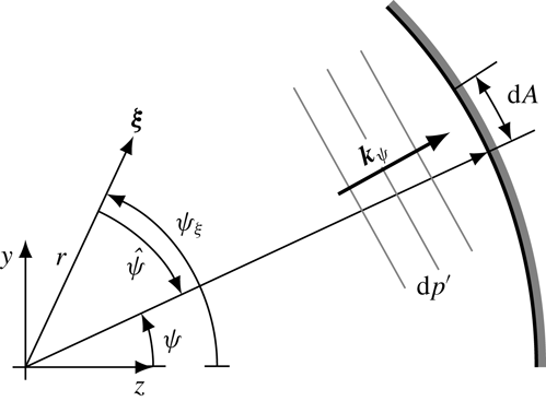
Sketch of an incremental plane wave. The origin of the coordinate system is located on the wind tunnel centreline and the outer arc represents the wall. The position vector
 $\unicode[STIX]{x1D743}=(x,y,z)^{T}$
and wave vector
 $\boldsymbol{k}_{\unicode[STIX]{x1D713}}$
are projected into the
 $y-z$
plane. Each wind tunnel wall increment
 $\text{d}A$
radiates an incremental plane acoustic wave. The resulting acoustic field can be obtained by circumferential integration of the incremental waves.

3 Axisymmetric superposition of inclined slow acoustic waves
The fundamental idea is based on the superposition of plane waves radiated by the turbulent boundary layer of a cylindrical nozzle wall. Each tunnel wall increment
 $\text{d}A$
located at the circumferential angle
 $\unicode[STIX]{x1D713}$
is presumed to radiate a plane acoustic wave of strength
 $|\text{d}p^{\prime }|\propto \text{d}A$
possessing the wave vector
 $\boldsymbol{k}_{\unicode[STIX]{x1D713}}$
as sketched in figure 4. Using
 $\text{d}A\propto \text{d}\unicode[STIX]{x1D713}$
, the pressure fluctuation induced by an incremental wave at the position
 $\unicode[STIX]{x1D743}=(x,y,z)^{T}$
and time
 $t$
can be written
 $$\begin{eqnarray}\text{d}p^{\prime }\propto \frac{1}{2\unicode[STIX]{x03C0}}\text{e}^{\text{i}(\boldsymbol{k}_{\unicode[STIX]{x1D713}}\boldsymbol{\cdot }\unicode[STIX]{x1D743}-\unicode[STIX]{x1D714}t)}\,\text{d}\unicode[STIX]{x1D713}.\end{eqnarray}$$
For convenience, the amplitude is defined as a small portion of the free stream pressure
 $\unicode[STIX]{x1D716}p_{\infty }$
and (3.1) is reformulated
 $$\begin{eqnarray}\text{d}p^{\prime }=\frac{\unicode[STIX]{x1D716}p_{\infty }}{2\unicode[STIX]{x03C0}}\text{e}^{\text{i}(\boldsymbol{k}_{\unicode[STIX]{x1D713}}\boldsymbol{\cdot }\unicode[STIX]{x1D743}-\unicode[STIX]{x1D714}t)}\,\text{d}\unicode[STIX]{x1D713}.\end{eqnarray}$$
The perturbations of the free stream pressure field follow from circumferential integration of (3.2)
 $$\begin{eqnarray}p^{\prime }=\frac{\unicode[STIX]{x1D716}p_{\infty }}{2\unicode[STIX]{x03C0}}\mathop{\oint }_{0}^{2\unicode[STIX]{x03C0}}\text{e}^{\text{i}(\boldsymbol{k}_{\unicode[STIX]{x1D713}}\boldsymbol{\cdot }\unicode[STIX]{x1D743}-\unicode[STIX]{x1D714}t)}\,\text{d}\unicode[STIX]{x1D713}.\end{eqnarray}$$
The wave vector can be formulated in terms of an axial and radial wavenumber
 $\boldsymbol{k}_{\unicode[STIX]{x1D713}}=(k_{x},k_{r}\sin (\unicode[STIX]{x1D713}),k_{r}\cos (\unicode[STIX]{x1D713}))^{T}$
whose values depend on the frequency and inclination angle
 $\unicode[STIX]{x1D719}$
related by the dispersion relation (2.3). Introducing
 $\unicode[STIX]{x1D713}=\unicode[STIX]{x1D713}_{\unicode[STIX]{x1D709}}+\hat{\unicode[STIX]{x1D713}}$
and
 $\unicode[STIX]{x1D743}=(x,r\sin (\unicode[STIX]{x1D713}_{\unicode[STIX]{x1D709}}),r\cos (\unicode[STIX]{x1D713}_{\unicode[STIX]{x1D709}}))^{T}$
, we obtain
 $$\begin{eqnarray}p^{\prime }=\frac{\unicode[STIX]{x1D716}p_{\infty }}{2\unicode[STIX]{x03C0}}\text{e}^{\text{i}(k_{x}x-\unicode[STIX]{x1D714}t)}\mathop{\oint }_{0}^{2\unicode[STIX]{x03C0}}\text{e}^{\text{i}k_{r}r\cos (\hat{\unicode[STIX]{x1D713}})}\,\text{d}\hat{\unicode[STIX]{x1D713}}.\end{eqnarray}$$
For the density perturbation the isentropic relation
 $\unicode[STIX]{x1D70C}^{\prime }=p^{\prime }/a^{2}$
holds. The axial and radial velocity fluctuations follow from integration of
 $$\begin{eqnarray}\displaystyle & \displaystyle \text{d}u_{x}^{\prime }=-\text{cos}(\unicode[STIX]{x1D719})(\unicode[STIX]{x1D70C}_{\infty }a_{\infty })^{-1}\,\text{d}p^{\prime } & \displaystyle\end{eqnarray}$$
 $$\begin{eqnarray}\displaystyle & \displaystyle \text{d}u_{r}^{\prime }=-\!\sin (\unicode[STIX]{x1D719})(\sin (\unicode[STIX]{x1D713})\sin (\unicode[STIX]{x1D713}_{\unicode[STIX]{x1D709}})+\cos (\unicode[STIX]{x1D713})\cos (\unicode[STIX]{x1D713}_{\unicode[STIX]{x1D709}}))(\unicode[STIX]{x1D70C}_{\infty }a_{\infty })^{-1}\,\text{d}p^{\prime }. & \displaystyle\end{eqnarray}$$
The resulting acoustic perturbations do not depend on
 $\unicode[STIX]{x1D713}_{\unicode[STIX]{x1D709}}$
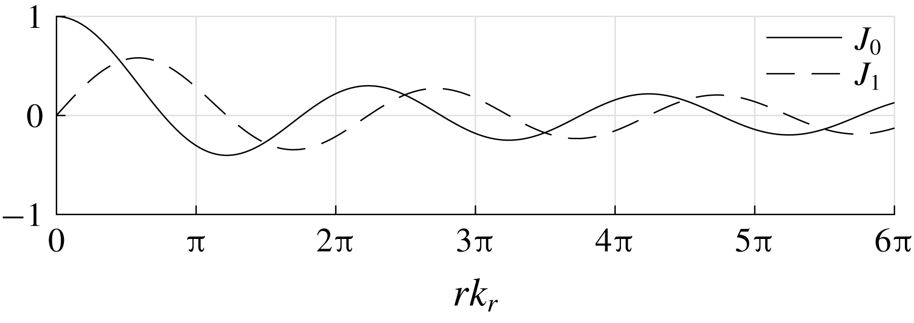
and can be expressed by Bessel functions of first kind. The complete disturbance field reads
 $$\begin{eqnarray}\displaystyle & \displaystyle p^{\prime }=\unicode[STIX]{x1D716}p_{\infty }\text{e}^{\text{i}(k_{x}x-\unicode[STIX]{x1D714}t)}J_{0}(k_{r}r) & \displaystyle\end{eqnarray}$$
 $$\begin{eqnarray}\displaystyle & \displaystyle \unicode[STIX]{x1D70C}^{\prime }=\frac{\unicode[STIX]{x1D716}p_{\infty }}{a_{\infty }^{2}}\text{e}^{\text{i}(k_{x}x-\unicode[STIX]{x1D714}t)}J_{0}(k_{r}r) & \displaystyle\end{eqnarray}$$
 $$\begin{eqnarray}\displaystyle & \displaystyle u_{x}^{\prime }=\frac{-\unicode[STIX]{x1D716}p_{\infty }}{\unicode[STIX]{x1D70C}_{\infty }a_{\infty }}\cos (\unicode[STIX]{x1D719})\text{e}^{\text{i}(k_{x}x-\unicode[STIX]{x1D714}t)}J_{0}(k_{r}r) & \displaystyle\end{eqnarray}$$
 $$\begin{eqnarray}\displaystyle & \displaystyle u_{r}^{\prime }=\frac{-\unicode[STIX]{x1D716}p_{\infty }\text{i}}{\unicode[STIX]{x1D70C}_{\infty }a_{\infty }}\sin (\unicode[STIX]{x1D719})\text{e}^{\text{i}(k_{x}x-\unicode[STIX]{x1D714}t)}J_{1}(k_{r}r). & \displaystyle\end{eqnarray}$$
The magnitudes of the radial distribution of pressure, density and velocity perturbations are sketched in figure 5 in terms of the corresponding Bessel function. Since both distributions are real valued, the incremental plane waves radially superpose to a standing wave. In time, there is a phase shift of
 $\unicode[STIX]{x03C0}/2$
between both types of distributions whose sign depends on the inclination angle via
 $-\text{sin}(\unicode[STIX]{x1D719})\text{i}$
. At
 $r=0$
, all plane waves have identical phase and interfere to maximal pressure fluctuations. The radial velocity vanishes at
 $r=0$
. Axially, the noise propagates with the common phase velocity of each increment
 $\unicode[STIX]{x1D714}/k_{x}$
.
Pressure and velocity distribution of the superposed inclined slow acoustic waves. The pressure, density and axial velocity magnitude distributions are prescribed by the Bessel function of first kind and zeroth order
 $J_{0}$
. The radial velocity magnitude distribution can be expressed by the Bessel function of first kind and first order
 $J_{1}$
. In time, there is a phase shift of
 $\unicode[STIX]{x03C0}/2$
between both types of distributions shown in (3.10).

The analysis of the resulting disturbances downstream of the shock wave is not as straightforward as for incident waves at zero angle of inclination. At any position in the flow field, the perturbation is a superposition of the contributions of all incremental plane waves. For an incremental plane wave, the transfer function in (2.12) is expressed via the complex non-dimensional transfer function
 $r_{p}(\unicode[STIX]{x1D743})$
 $$\begin{eqnarray}r_{p}=\frac{\text{d}p^{\prime }}{p_{t}}\frac{\unicode[STIX]{x1D70C}_{\infty }}{\text{d}\unicode[STIX]{x1D70C}_{\infty }^{\prime }}.\end{eqnarray}$$
Using the ansatz (3.2), the equation of state for an ideal gas
 $\unicode[STIX]{x1D70C}=\unicode[STIX]{x1D6FE}p/a^{2}$
, the identity
 $\text{d}\hat{\unicode[STIX]{x1D713}}=\text{d}\unicode[STIX]{x1D713}$
, and
 $\unicode[STIX]{x1D70C}^{\prime }=p^{\prime }/a^{2}$
for an acoustic wave, (3.11) can be rewritten to
 $$\begin{eqnarray}r_{p}=\frac{2\unicode[STIX]{x03C0}\unicode[STIX]{x1D6FE}}{p_{t}\unicode[STIX]{x1D716}}\,\frac{\text{d}p^{\prime }}{\text{d}\hat{\unicode[STIX]{x1D713}}}.\end{eqnarray}$$
Note that the time dependence
 $\exp (-\text{i}\unicode[STIX]{x1D714}t)$
cancels and the complexity of
 $r_{p}$
accounts for the phase shift in space. The determination of the integral transfer functions requires probe surface averaged data to account for the radial wavenumber of the flow disturbances. The complex averaged transfer function
 $\overline{r}_{p}$
is defined
 $$\begin{eqnarray}\overline{r}_{p}=\frac{1}{\unicode[STIX]{x03C0}r_{e}^{2}}\int _{0}^{r_{e}}\mathop{\oint }_{0}^{2\unicode[STIX]{x03C0}}r_{p}\,\text{d}\hat{\unicode[STIX]{x1D713}}r\,\text{d}r,\end{eqnarray}$$
 $r_{e}$
being the extent of the area of averaging. Eliminating the inner integral in (3.13) by using (3.12), the integral transfer function can be rewritten
 $$\begin{eqnarray}\overline{r}_{p}=\frac{2\unicode[STIX]{x1D6FE}}{\unicode[STIX]{x1D716}r_{e}^{2}}\int _{0}^{r_{e}}\frac{p^{\prime }}{p_{t}}r\,\text{d}r.\end{eqnarray}$$
The radial distribution of perturbed pressure is the circumferential integral over
 $\text{d}\unicode[STIX]{x1D713}$
, i.e. all incremental plane waves for
 $\unicode[STIX]{x1D713}_{\unicode[STIX]{x1D709}}=\text{const}$
. In other words, it also denotes the circumferential integral over
 $\text{d}\unicode[STIX]{x1D713}_{\unicode[STIX]{x1D709}}$
of a single incremental plane wave for
 $\unicode[STIX]{x1D713}=\text{const}$
. It cannot be decomposed into the circumferential distribution of a single incremental wave. On the axis of rotation, the transfer function
 $r_{p}$
does not depend on
 $\hat{\unicode[STIX]{x1D713}}$
, i.e. all waves contribute in phase, and therefore, (3.12) can be integrated directly and solved for the transfer function of inclined incident waves at the stagnation point to
 $$\begin{eqnarray}r_{p}=\frac{p^{\prime }\unicode[STIX]{x1D6FE}}{p_{t}\unicode[STIX]{x1D716}}.\end{eqnarray}$$
Note that the transfer functions
 $r_{p}$
and
 $\overline{r}_{p}$
are complex numbers. Thus, the desired ratio of free stream to postshock amplitude is the absolute value of
 $r_{p}$
and
 $\overline{r}_{p}$
. The complex pressure distribution
 $p^{\prime }$
in (3.14) and (3.15) can be obtained by performing a discrete Fourier transform of the DNS results.
To analyse the response of the probe to a single pulse of (3.4) and (3.8) to (3.10), the phase
 $\unicode[STIX]{x1D711}=\boldsymbol{k}_{\unicode[STIX]{x1D713}}\boldsymbol{\cdot }\unicode[STIX]{x1D743}-\unicode[STIX]{x1D714}t$
in (3.2) is processed by the filter function
 $f(\unicode[STIX]{x1D711})$
. A single pulse is contained in
 $\unicode[STIX]{x0394}\unicode[STIX]{x1D711}=\unicode[STIX]{x03C0}$
and for the ansatz (3.2) the filter function is
 $$\begin{eqnarray}f(\unicode[STIX]{x1D711})=\left\{\begin{array}{@{}ll@{}}\unicode[STIX]{x1D711}-\unicode[STIX]{x1D711}_{0}+\unicode[STIX]{x03C0}/2, & \text{if }\unicode[STIX]{x1D711}_{0}-\unicode[STIX]{x03C0}<\unicode[STIX]{x1D711}<\unicode[STIX]{x1D711}_{0},\\ \unicode[STIX]{x03C0}/2, & \text{else},\end{array}\right.\end{eqnarray}$$
with
 $\unicode[STIX]{x1D711}_{0}=\min (\boldsymbol{k}_{\unicode[STIX]{x1D713}}\boldsymbol{\cdot }\unicode[STIX]{x1D743})-\unicode[STIX]{x1D714}t_{0}$
. The pulse enters the domain at the most upstream position with respect to the pulse propagation at the time of insertion
 $t_{0}$
. The filtered equivalent of (3.4)
 $$\begin{eqnarray}p^{\prime }=\frac{\unicode[STIX]{x1D716}p_{\infty }}{2\unicode[STIX]{x03C0}}\mathop{\oint }_{0}^{2\unicode[STIX]{x03C0}}\text{e}^{\text{i}f(k_{x}x-\unicode[STIX]{x1D714}t+k_{r}r\cos (\hat{\unicode[STIX]{x1D713}}))}\,\text{d}\hat{\unicode[STIX]{x1D713}}\end{eqnarray}$$
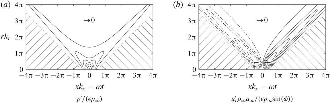
describes the perturbation of the pressure field and is depicted in figure 6(a) as a function of radial
 $rk_{r}$
and axial–temporal
 $xk_{x}-\unicode[STIX]{x1D714}t$
phase contribution. Since the real part of the integrand of (3.17) is larger or equal to zero in the range of
 $f(\unicode[STIX]{x1D711})$
, only positive pressure perturbations occur. For
 $xk_{x}-\unicode[STIX]{x1D714}t\geqslant rk_{r}+\unicode[STIX]{x03C0}/2$
and
 $xk_{x}-\unicode[STIX]{x1D714}t\leqslant -(rk_{r}+\unicode[STIX]{x03C0}/2)$
no fluctuations arise, i.e. the wave either did not reach the region yet or already passed. Both regions are shaded and confined by dotted lines. Between these limiting regions the pressure distribution is non-zero. For
 $rk_{r}-\unicode[STIX]{x03C0}/2\leqslant xk_{x}-\unicode[STIX]{x1D714}t\leqslant \unicode[STIX]{x03C0}/2-rk_{r}$
, i.e. in the vicinity of
 $rk_{r}=0$
and
 $xk_{x}-\unicode[STIX]{x1D714}t=0$
where all incremental waves interfere constructively to the highest pressure fluctuation, the filter is not effective and the Bessel function
 $J_{0}$
can be used to calculate (3.17). In the remaining
 $rk_{r}-xk_{x}-\unicode[STIX]{x1D714}t$
space, the filter suppresses contributions from incremental plane waves radiated in certain regions
 $\unicode[STIX]{x0394}\hat{\unicode[STIX]{x1D713}}$
, i.e. the filter function can be shifted to the limits of the integral to allow efficient numerical integration. The two branches evident in the pressure distribution can be related to superposing incremental plane waves from the region in the vicinity of
 $\hat{\unicode[STIX]{x1D713}}=0$
on the left and
 $\hat{\unicode[STIX]{x1D713}}=\unicode[STIX]{x03C0}$
on the right. Furthermore, interpreting the
 $rk_{r}$
axis as a
 $yk_{y}$
axis, the left branch resembles the continuation of the right branch at negative values of
 $y$
.
Pressure and velocity distribution generated by a single pulse according to (3.17) and (3.18) as a function of radial
 $rk_{r}$
and axial–temporal
 $xk_{x}-\unicode[STIX]{x1D714}t$
wavenumber: (a) no pressure fluctuations occur in the shaded area below the dotted lines; in between, the solid lines denote multiples of
 $0.15$
and the maximum at
 $(0,0)$
is
 $1$
; (b) the radial velocity perturbations vanish in the shaded area and possess positive (solid) and negative (broken) values, the lines denote multiples of
 $0.05$
and the extrema are approximately
 $\pm 0.3011$
at
 $(\pm 0.3525\unicode[STIX]{x03C0},0.4225\unicode[STIX]{x03C0})$
obtained by numerical integration.

Density and axial velocity perturbations are related to the pressure fluctuation as in (3.8) and (3.9). The filtered radial velocity distribution
 $$\begin{eqnarray}u_{r}^{\prime }=\frac{-\unicode[STIX]{x1D716}p_{\infty }}{2\unicode[STIX]{x03C0}\unicode[STIX]{x1D70C}_{\infty }a_{\infty }}\sin (\unicode[STIX]{x1D719})\mathop{\oint }_{0}^{2\unicode[STIX]{x03C0}}\cos (\hat{\unicode[STIX]{x1D713}})\text{e}^{\text{i}f(k_{x}x-\unicode[STIX]{x1D714}t+k_{r}r\cos (\hat{\unicode[STIX]{x1D713}}))}\,\text{d}\hat{\unicode[STIX]{x1D713}}\end{eqnarray}$$
is confined in figure 6(b) by the identical relations of
 $rk_{r}$
and
 $xk_{x}-\unicode[STIX]{x1D714}t$
. The velocity distribution of both branches has an opposing sign due to the additional term
 $\cos (\hat{\unicode[STIX]{x1D713}})$
assigning a negative sign to velocity fluctuations from
 $\unicode[STIX]{x03C0}/2<\hat{\unicode[STIX]{x1D713}}<3\unicode[STIX]{x03C0}/2$
in the integrand of (3.18). The interpretation of the branches is analogous to the pressure perturbation, where the change of sign follows from the transformation of the radial velocity to the velocity fluctuation in the
 $y$
-direction.
Like for the unfiltered continuous formulation, the pressure perturbation caused by an incremental plane wave at
 $r=0$
and circumferentially averaged quantities can be obtained by the axisymmetric boundary condition. For the filtered formulation, real valued time dependent pressure transfer functions
 $r_{p}(x,r=0,t)$
and
 $\overline{r}_{p}(x,r_{e},t)$
are defined as in (3.14) and (3.15) and will be employed to investigate the response of the SPP to single pulses of inclined waves.
Thus, although the dimensions of the original problem are reduced, no approximations are introduced and the obtained transfer functions are exact as long as linearity is ensured. Linearity was shown to prevail by Chaudhry & Candler (Reference Chaudhry and Candler2017) and was also found in the present results and Schilden & Schröder (Reference Schilden and Schröder2017). In the following, the set-up and the results of corresponding DNS are presented.
4 Computational set-up
The numerical method and the flow configuration are identical to Schilden & Schröder (Reference Schilden and Schröder2017) which is why they are only briefly described.
The DNS are based on the three-dimensional Navier–Stokes equations. The system of equations is closed by the equation of state for an ideal gas. For air, the ratio of specific heats is
 $\unicode[STIX]{x1D6FE}=1.4$
and the Prandtl number is
 $0.72$
. The governing equations are approximated by a finite-volume unstructured Cartesian grid method (Hartmann, Meinke & Schröder Reference Hartmann, Meinke and Schröder2008; Lintermann et al.
Reference Lintermann, Schlimpert, Grimmen, Günther, Meinke and Schröder2014; Schneiders et al.
Reference Schneiders, Günther, Meinke and Schröder2016). For supersonic flows, the numerical method has been employed and validated for the flow past a cone (Schilden et al.
Reference Schilden, Schröder, Ali, Wu, Schreyer and Radespiel2016) and around blunt bodies, e.g. the SPP in Schilden & Schröder (Reference Schilden and Schröder2017) and a re-entry capsule in Hein et al. (Reference Hein, Theiss, Di Giovanni, Schilden, Schröder, Paredes, Choudhari, Li and Reshotko2018).
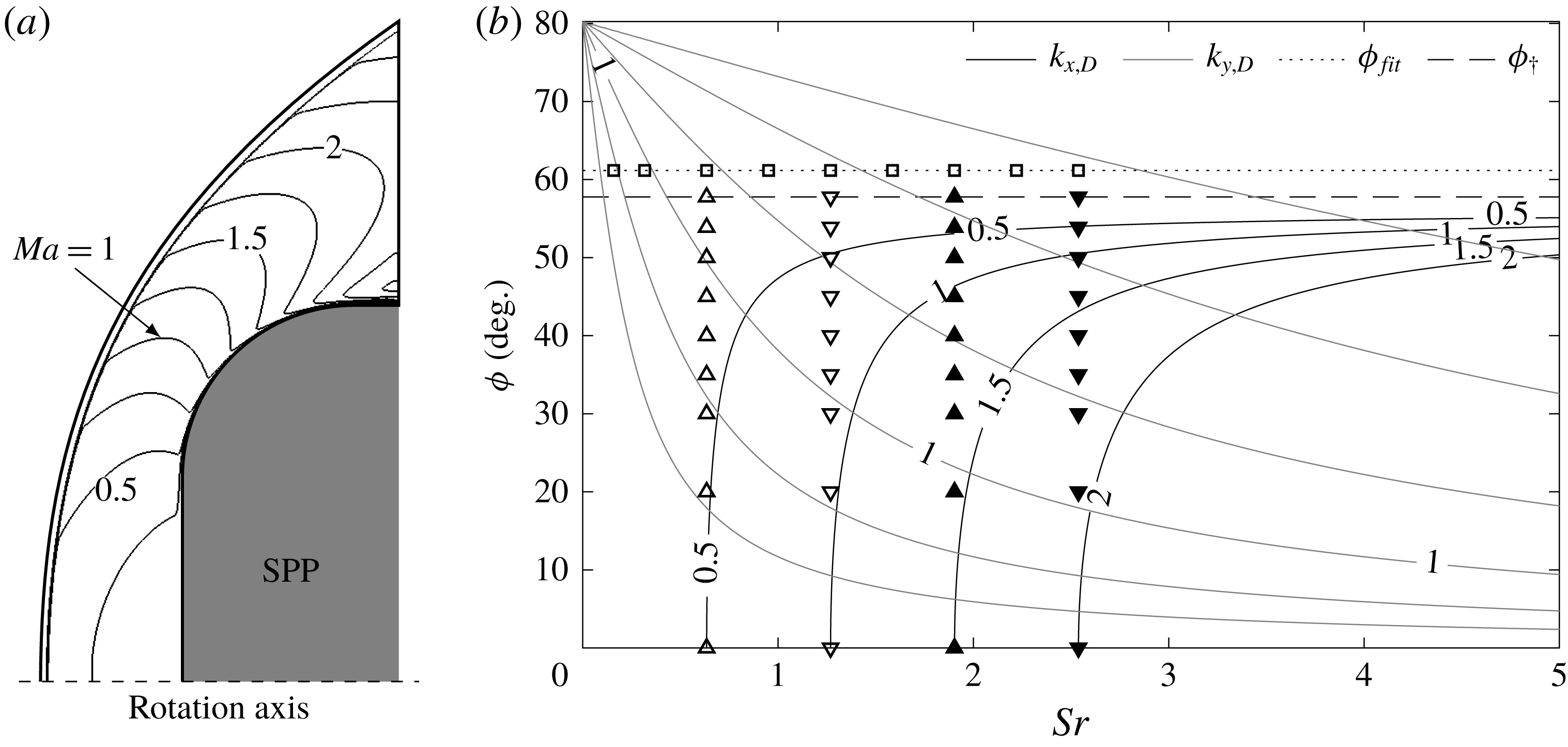
Unperturbed flow field from Schilden & Schröder (Reference Schilden and Schröder2017) and cases of perturbed flow: (a) lines of constant Mach number of the unperturbed flow downstream of the shock wave,
 $\unicode[STIX]{x0394}Ma=0.25$
between the isolines; (b) cases of the investigation in the non-dimensional wavenumber map. The axial wavenumber is scaled according to (5.1). ▫: acoustic waves at
 $\unicode[STIX]{x1D719}=61.16^{\circ }$
inclination representing noise radiated by a turbulent boundary layer. ▵: acoustic waves at
 $Sr_{3}=0.634\,(72.1\,\text{kHz})$
; at
 $\unicode[STIX]{x1D719}=0^{\circ }$
this Strouhal number defined the first peak of constructive interference. ▿: acoustic waves at
 $Sr_{5}=1.269\,(144.1~\text{kHz})$
; at
 $\unicode[STIX]{x1D719}=0^{\circ }$
this Strouhal number defined the first valley of destructive interference. ▴: acoustic waves at
 $Sr_{7}=1.904\,(216.2~\text{kHz})$
; at
 $\unicode[STIX]{x1D719}=0^{\circ }$
this Strouhal number defined the second peak of constructive interference. ▾: acoustic waves at
 $Sr_{9}=2.538\,(288.3~\text{kHz})$
; at
 $\unicode[STIX]{x1D719}=0^{\circ }$
this Strouhal number defined the second valley of destructive interference.

The free stream is assumed laminar at a Mach number
 $Ma=5.9$
. The SPP is schematically shown in figure 7(a) and the axis of rotation is aligned with the flow. The Reynolds numbers based on the diameter is
 $Re_{D}=50\,000$
. In the experiments of Ali et al. (Reference Ali, Zárate Cárdenas, Radespiel, Schilden and Schröder2018), the probe is equipped with a PCB pressure transducer having a rectangular sensor area. In the axisymmetric context, the transducer extent is approximated by a circle having the same area and the outer radius is
 $r_{e}/D=0.0564$
. Since the flow is axisymmetric, a periodic boundary condition formulation for Cartesian meshes by Pogorelov, Meinke & Schröder (Reference Pogorelov, Meinke and Schröder2015) is used to reduce the circumferential extent of the three-dimensional computational domain to a small segment. The axisymmetric inclined slow acoustic waves of § 3 are imposed on the free stream upstream of the detached shock wave.
Furthermore, DNS based on the two-dimensional Navier–Stokes equations are included in the analysis. The plane configuration of the SPP resembles a blunt leading edge of a plate. In these simulations, the complete flow between the shock and the SPP is resolved, i.e. symmetry is not exploited, and inclined slow acoustic waves can be directly imposed on the free stream. The data are denoted ‘2D SPP’.
5 Results
For the sake of clarity, the most important features of the unperturbed flow from Schilden & Schröder (Reference Schilden and Schröder2017) are summarised, first. Please refer to the original source for more information. Second, the perturbed flow solutions are discussed.
5.1 Unperturbed flow
The supersonic velocity field around the blunt SPP is characterised by the detached bow shock and the large subsonic region downstream of the shock wave. Figure 7(a) shows the Mach number contours. Close to the inflow they all collapse and show the location of the shock wave. The flow in the subsonic region downstream of the bow shock is accelerated to supersonic speed half-way along the rounded edge. At the outflow downstream of the shock wave Mach numbers of approximately
 $2.5$
are reached.
From the distributions of the axial velocity and speed of sound between shock wave and stagnation point along the axis of rotation an a priori estimate of the acoustic standoff frequency can be calculated for the duration
 $t_{sa}+t_{fa}$
of a non-inclined acoustic wave travelling upstream from the stagnation point to the shock wave as a slow acoustic wave and then back to the stagnation point as a fast acoustic wave. From
 $t_{ac}=t_{sa}+t_{fa}$
, the shock standoff Strouhal number can be computed to be
 $Sr_{ac}=1.269\,(144.1~\text{kHz})$
.
For the two-dimensional plane configuration, the shock standoff distance is larger since it lacks the circumferential direction for the postshock flow to diverge in increasing normal coordinate direction, i.e. the radius
 $r$
in axisymmetric flow. Therefore,
 $t_{ac}$
is larger than in three-dimensional axisymmetric flow and the shock standoff Strouhal number is
 $Sr_{ac}=0.578\,(65.58~\text{kHz})$
.
5.2 Perturbed flow
Numerical simulations are performed for selected Strouhal numbers
 $Sr$
and wave inclination angles
 $\unicode[STIX]{x1D719}$
. An overview in the wavenumber map is given in figure 7(b). Note that the postshock axial wavenumber (2.10) is scaled by the postshock axial wavenumber at the first valley of destructive interference for non-inclined incident waves and reads
 $$\begin{eqnarray}\tilde{k}_{x,D}=\frac{k_{x,D}}{k_{x,D,ac}}.\end{eqnarray}$$
First, the Strouhal number dependence of the transfer functions
 $r_{p}$
and
 $\overline{r}_{p}$
is investigated for waves at high angles of inclination marked as squares in figure 7(b). The angle of inclination
 $61.16^{\circ }$
was chosen based on (2.6) and (2.7) for
 $Ma=5.9$
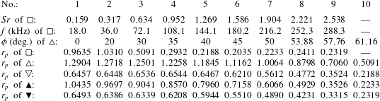
and thus represents acoustic waves radiated by a supersonic boundary layer. The Strouhal numbers reach up to the second Strouhal number of destructive interference of non-inclined acoustic waves and are summarised in table 1. The fifth Strouhal number
 $Sr_{5}$
is the shock standoff Strouhal number
 $Sr_{ac}$
. The remaining triangle marker cases in figure 7(b) cover four characteristic Strouhal numbers of de- and constructive interference for non-inclined incident waves and inclination angles from zero to radiation inclination, i.e. the cases at radiation inclination in line with the triangle cases are included. The inclination angles are listed in table 1. The last but one inclination angle is the critical angle of incidence for normal shock waves
 $\unicode[STIX]{x1D719}_{\dagger }$
of (2.11). The Strouhal numbers of the triangle marker cases are
 $Sr_{3}=0.634$
,
 $Sr_{5}=1.269$
,
 $Sr_{7}=1.904$
and
 $Sr_{9}=2.538$
. The vertical alignment of the triangle markers indicate the type of interference, i.e. upward facing triangles for peaks and downward facing triangles for valleys of the transfer function of non-inclined incident waves. Furthermore, simulations of single pulses of inclined acoustic waves are performed for all cases at
 $Sr_{3}$
,
 $Sr_{5}$
,
 $Sr_{7}$
and
 $Sr_{9}$
.
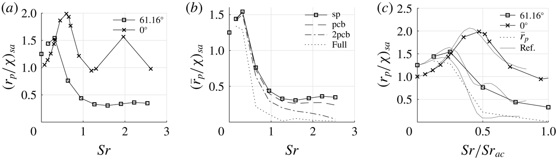
Transfer functions
 $r_{p}$
and
 $\overline{r}_{p}$
scaled by the low frequency limit of non-inclined slow acoustic waves
 $\unicode[STIX]{x1D712}_{sa}$
: (a) comparison of stagnation point data
 $r_{p}$
of radiated acoustic waves ‘
 $61.16^{\circ }$
’ to non-inclined cases ‘
 $0^{\circ }$
’ from Schilden & Schröder (Reference Schilden and Schröder2017) plus further lower Strouhal number results, the disconnected square at
 $Sr=0$
is the low frequency limit of (2.14); (b) comparison of
 $r_{p}$
at the stagnation point ‘sp’ to surface averaged transfer functions
 $\overline{r}_{p}$
, ‘pcb’ denotes averaging over the sensitive are of the pressure transducer, ‘2pcb’ has twice the size, and ‘Full’ denotes the complete flat front of the SPP; (c) comparison of the transfer functions
 $r_{p}$
and
 $\overline{r}_{p}$
with reference data ‘Ref’ from Duan et al. (Reference Duan, Choudhari, Chou, Muñoz, Ali, Radespiel, Schilden, Schröder, Marineau and Casper2018).

Strouhal numbers
 $Sr$
and inclination angles
 $\unicode[STIX]{x1D719}$
of the investigated cases shown in figure 7(b). Strouhal numbers and frequency of the cases marked as squares at
 $\unicode[STIX]{x1D719}=61.16^{\circ }$
. The inclination angles
 $\unicode[STIX]{x1D719}$
belong to the triangle marker cases at
 $Sr_{3}=0.634$
,
 $Sr_{5}=1.269$
,
 $Sr_{7}=1.904$
and
 $Sr_{9}=2.538$
. The values of the transfer functions
 $r_{p}$
of all the cases from figure 7(b) are given.

5.2.1 Frequency response: acoustic waves radiated by a turbulent boundary layer
The transfer functions
 $r_{p}$
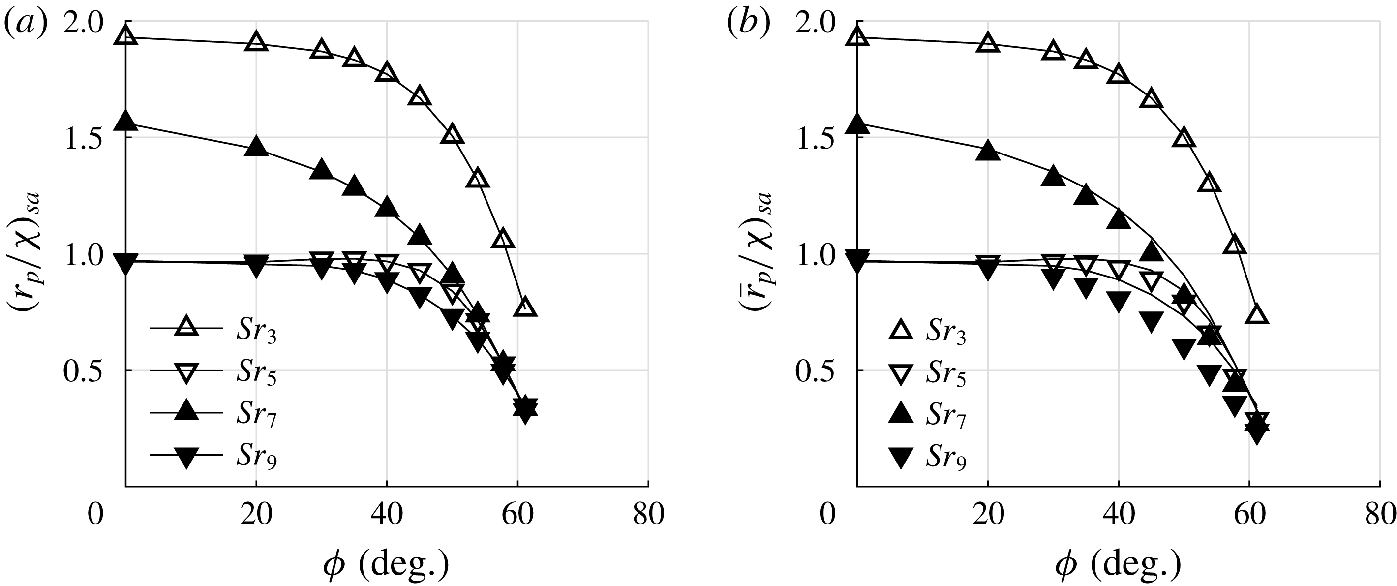
for acoustic waves radiated by the turbulent boundary layer and the effect of surface averaging are shown in figure 8. In figure 8(a), the stagnation point data
 $r_{p}$
are compared to the non-inclined cases from Schilden & Schröder (Reference Schilden and Schröder2017). In Schilden & Schröder (Reference Schilden and Schröder2017), the present and one higher Reynolds number were investigated. The Reynolds number effect on the pressure transfer function was negligible and therefore both datasets are combined. The resonant behaviour defined by constructive interference at
 $Sr=0.634$
and
 $Sr=1.904$
and destructive interference at
 $Sr=1.269$
and
 $Sr=2.538$
is evident. Furthermore, lower Strouhal number cases – not included in the aforementioned paper – are added. The square at
 $Sr=0$
denotes the low frequency limit of (2.14) for the wave inclination angle
 $\unicode[STIX]{x1D719}=61.16^{\circ }$
. As expected from the derivation of the low frequency limit, the transfer function of highly inclined acoustic waves exceeds that of the non-inclined cases at low Strouhal numbers. It is evident from figure 7(b) that an expression for the range of validity of the reduced-order method cannot be provided. The effect of the inclination angle is later discussed for Strouhal numbers
 ${>}0.634\,(Sr_{3})$
. For these Strouhal numbers, the transfer functions for
 $\unicode[STIX]{x1D719}=0^{\circ }$
and
 $\unicode[STIX]{x1D719}=61.16^{\circ }$
in figure 8(a) are highly influenced by transient effects. Starting from the low frequency limit, the transfer function further increases for higher Strouhal number. After peaking at a low Strouhal number having a lower maximum transfer function than the non-inclined data, the transfer function decays and remains at approximately
 $r_{p}/\unicode[STIX]{x1D712}\approx 0.35$
for Strouhal numbers
 $Sr>1$
. Near
 $Sr=2$
another slight increase is observed.
Since pressure transducers have a finite extent of sensitive area, the distribution of
 $r_{p}$
over the respective area needs to be averaged according to (3.14). In figure 8(b), the stagnation point transfer function
 $r_{p}$
is compared to three radial extents of averaging. For the PCB pressure transducer used by Ali et al. (Reference Ali, Zárate Cárdenas, Radespiel, Schilden and Schröder2018) denoted by ‘pcb’, the averaging effect starts to be visible at approximately
 $Sr\approx 1$
and is moderate in the higher Strouhal number range of the investigation. The value at the highest Strouhal number reduces to
 $68\,\%$
of the stagnation point value. For a sensitive area with twice the radius ‘2pcb’, averaging effects are evident over the whole Strouhal number range and the maximum decrease is up to
 $12\,\%$
. When the pressure fluctuations from the complete flat surface of the SPP are averaged, the averaging effect is intense for Strouhal numbers
 $Sr>0.5$
and evident for low Strouhal numbers, where higher values than the low frequency limit still occur.
Moreover, in figure 8(c), a comparison to a result of three-dimensional DNS in Duan et al. (Reference Duan, Choudhari, Chou, Muñoz, Ali, Radespiel, Schilden, Schröder, Marineau and Casper2018) of a similar configuration is shown. The reference data ‘Ref’ are for a cylindrical SPP in
 $Ma=6$
flow and inclined slow acoustic waves at
 $\unicode[STIX]{x1D719}=0^{\circ }$
and
 $\unicode[STIX]{x1D719}=60^{\circ }$
angle of incidence. The transfer function on the ordinate is scaled by the low frequency limit for non-inclined slow acoustic waves, i.e. the Mach number difference is accounted for. To consider the different geometry, i.e. the flow field possesses a different shock standoff distance, the Strouhal number on the abscissa is scaled by the shock standoff Strouhal number which is approximately
 $Sr_{ac}\approx 0.92$
for the data in Duan et al. (Reference Duan, Choudhari, Chou, Muñoz, Ali, Radespiel, Schilden, Schröder, Marineau and Casper2018). The non-inclined cases
 $\unicode[STIX]{x1D719}=0^{\circ }$
compare well. The flow is axisymmetric and neither method relies on further assumptions concerning the numerical method. At the inclination of radiated waves
 $\unicode[STIX]{x1D719}\approx 60^{\circ }$
, the comparison shows good agreement of the transfer function obtained in three-dimensional and the axisymmetric simulations. The normalisation used for the comparison was proposed by Chaudhry & Candler (Reference Chaudhry and Candler2017) for non-inclined incident waves but seems to also hold at high inclination angles. Also the averaging effect is captured well in
 $\overline{r}_{p}$
. Note that the data in Duan et al. (Reference Duan, Choudhari, Chou, Muñoz, Ali, Radespiel, Schilden, Schröder, Marineau and Casper2018) are averaged over
 $96\,\%$
of the radial extent while the flat surface of the SPP extends to
 $54\,\%$
. Due to this good agreement, the axisymmetric boundary condition derived in § 3 is considered appropriate. Furthermore, the results were tested with respect to grid convergence, see figure 12(b), and linearity which is the only assumption in the derivation of the axisymmetric boundary condition. Considering the aforementioned expression for the validity range of the low frequency limit of the transfer function, figure 8(c) suggests a formulation based on
 $Sr/Sr_{ac}$
.
At this point, the calibration of the SPP for the measurement of acoustic waves radiated by a
 $Ma=5.9$
boundary layer is completed. It can be concluded that the transfer function for highly inclined waves drops drastically at approximately
 $Sr\approx 0.5$
. In this Strouhal number region, the transfer function depends strongly on the Strouhal number. Furthermore, the
 $r_{p}$
range is wider than for the non-inclined wave. There is a ratio of
 $4.73$
of the highest and lowest value. These properties of
 $r_{p}$
necessitate experimental data in the form of power spectral density (PSD) distributions or bandwidth filtered nRMS values to accurately compute free stream tunnel noise. Broad bandwidth filtered data in the vicinity of
 $Sr\approx 0.5$
should be avoided.
Compared to non-inclined fast acoustic waves, the
 $r_{p}$
values of the inclined radiated slow acoustic waves are smaller, especially at Strouhal numbers
 $Sr>1$
. The values of the non-inclined fast waves can be obtained by multiplying the ‘
 $0^{\circ }$
’ data in figure 8(a) with the low frequency limit ratio of non-inclined fast and slow acoustic waves
 $\unicode[STIX]{x1D712}_{fa}/\unicode[STIX]{x1D712}_{sa}$
of approximately two. For instance, at
 $Sr\approx 2$
, the
 $r_{p}$
of the non-inclined fast acoustic wave is one order of magnitude greater than the value for inclined radiated slow acoustic waves. Therefore, in the presence of non-inclined fast acoustic waves, e.g. progressive sound waves emanating from the subsonic part of the wind tunnel, the choice of transfer function has to be reconsidered since even in the case of dominating inclined disturbances, the weaker fast acoustic waves might contribute to the measured pressure fluctuations in the same order of magnitude.
Having compared the extreme cases, i.e. the non-inclined and highly inclined cases, the sensitivity to the inclination angle is investigated next.
5.2.2 Frequency response: effect of wave inclination
The impact of wave inclination at constant Strouhal numbers is depicted in figure 9. It shows how the transfer function decreases from the non-inclined waves to radiation inclination for four distinct Strouhal numbers, i.e. the Strouhal numbers of the first two maxima and minima of the transfer function of the non-inclined incident waves. The Strouhal numbers are given in table 1 and are denoted
 $0.5\,Sr_{ac}=Sr_{3}$
for the first maximum,
 $Sr_{ac}=Sr_{5}$
for the first minimum,
 $1.5\,Sr_{ac}=Sr_{7}$
for the second maximum, and
 $2\,Sr_{ac}=Sr_{9}$
for the second minimum. The stagnation point transfer function
 $r_{p}$
in figure 9(a) shows monotonically decreasing data except for cases at the Strouhal number of the first minimum
 $Sr_{5}$
. These data exhibit a local maximum at
 $\unicode[STIX]{x1D719}=35^{\circ }$
. On the contrary, the low frequency limit for inclined slow acoustic waves (2.14) increases monotonically from
 $\unicode[STIX]{x1D719}=0$
towards the Mach angle. Hence, between
 $Sr\rightarrow 0$
and
 $Sr=0.634$
the trend of
 $r_{p}$
over
 $\unicode[STIX]{x1D719}$
changes fundamentally. This statement is corroborated by figure 8(a) considering the higher
 $r_{p}$
values for inclined waves for Strouhal number up to
 $Sr=0.317$
and the following drastic decay.
Transfer functions
 $r_{p}$
and
 $\overline{r}_{p}$
of triangle cases from figure 7(b); (a) local data
 $r_{p}$
from the stagnation point; (b) averaged data
 $\overline{r}_{p}$
over the sensitive area of the PCB probe mounted inside the SPP, the lines represent
 $r_{p}$
of (a).

At small angles of inclination, the transfer function in figure 9(a) is not sensitive to the inclination angle, whereas at radiation inclination
 $|\text{d}r_{p}/\text{d}\unicode[STIX]{x1D719}|$
is significantly larger. For the four Strouhal numbers,
 $\text{d}r_{p}/\text{d}\unicode[STIX]{x1D719}<0$
holds and since the low frequency limit monotonically increases, the derivative is
 $\text{d}r_{p}/\text{d}\unicode[STIX]{x1D719}>0$
. Performing a Taylor series expansion of (2.12), the deviation of the free stream density fluctuation
 $\unicode[STIX]{x0394}\unicode[STIX]{x1D70C}_{\infty }^{\prime }/\unicode[STIX]{x1D70C}_{\infty }^{\prime }$
, i.e. the signed relative error, can be related to the uncertainty in the inclination angle
 $\unicode[STIX]{x0394}\unicode[STIX]{x1D719}$
by
 $$\begin{eqnarray}\frac{\unicode[STIX]{x0394}\unicode[STIX]{x1D70C}_{\infty }^{\prime }}{\unicode[STIX]{x1D70C}_{\infty }^{\prime }}=\frac{-1}{r_{p}}\,\frac{\text{d}r_{p}}{\text{d}\unicode[STIX]{x1D719}}\unicode[STIX]{x0394}\unicode[STIX]{x1D719}.\end{eqnarray}$$
For the Strouhal numbers in figure 9(a), the factor
 $(\text{d}r_{p}/\text{d}\unicode[STIX]{x1D719})/r_{p}$
can be approximated using the discrete data points. The low frequency limit (2.14) of
 $r_{p}$
can be used to analytically determine the corresponding value for
 $Sr\rightarrow 0$
. The values are tabulated in table 2 for
 $\unicode[STIX]{x1D719}=61.16^{\circ }$
. Towards
 $Sr\rightarrow 0$
, the error in the free stream density amplitude is
 ${<}1\,\%$
per degree uncertainty in
 $\unicode[STIX]{x1D719}$
. Compared to the higher Strouhal number data, the transfer function range of
 $\unicode[STIX]{x1D712}_{\unicode[STIX]{x1D719}}$
is narrow in the investigated inclination angle range. Scaled with the low frequency limit for non-inclined waves, the highest low frequency limit at radiation inclination is
 $\unicode[STIX]{x1D712}_{\unicode[STIX]{x1D719}}/\unicode[STIX]{x1D712}=1.25$
and thus, both elements of the error propagation estimate, i.e.
 $r_{p}^{-1}$
and the derivative, are benign. For the four Strouhal numbers, the propagation of uncertainty in the inclination angle towards the free stream disturbance amplitude is between
 $10$
and
 $20\,\%$
per degree error in
 $\unicode[STIX]{x1D719}$
. This means that the inclination angle is extremely important to determine the transfer function
 $r_{p}$
. This significance has to be considered to estimate the error of the calibration of the SPP, e.g. approximations or models like (2.7) and the uncertainty in the determination of the radiation angle in experiments and numerical simulations.
Transfer function
 $\overline{r}_{p}$
of triangle cases from figure 7(b) averaged over the entire flat front of the SPP, the lines represent
 $r_{p}$
of figure 9(a): (a) shown versus the inclination angle
 $\unicode[STIX]{x1D719}$
; (b) shown versus the radial wavenumber
 $k_{y,D}$
from (2.8).

Propagation of the uncertainty in the choice of inclination angle
 $\unicode[STIX]{x1D719}$
into the relative error of the free stream density amplitude
 $\unicode[STIX]{x1D70C}_{\infty }^{\prime }$
based on (5.2) at
 $\unicode[STIX]{x1D719}=61.16^{\circ }$
. For
 $Sr\rightarrow 0$
the value follows from (2.14) whereas the remaining values are calculated from the discrete data points in figure 9(a,b).

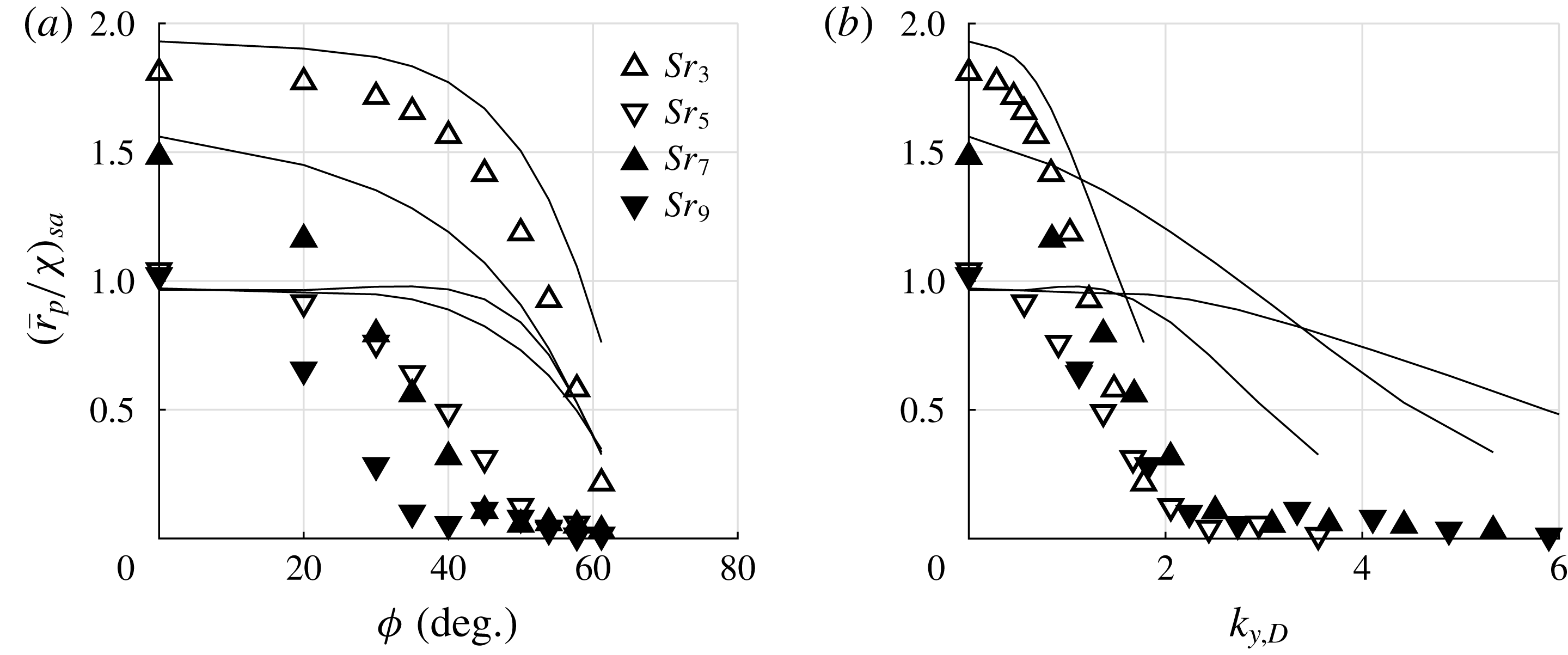
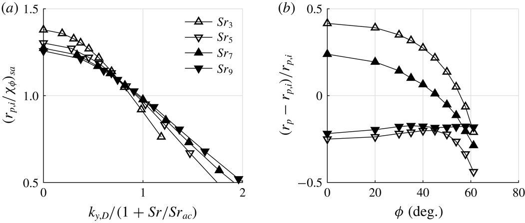
The effect of averaging on the detection of inclined waves is depicted in figure 9(b) for the PCB sensor and in figure 10(a) for the entire flat front of the SPP. Both figures show the averaged data as symbols and the local transfer functions of figure 9(a) are included as solid lines. Averaging over the active area of the PCB transducer has a moderate effect at inclination angles higher than
 $20^{\circ }$
for the highest Strouhal numbers. The propagation of uncertainty in the inclination angle towards the free stream disturbance amplitude considering the surface averaged data is shown in the second row of data in table 2 and shows a slight increase of the absolute value. This increase is small compared to the sensitivity of the stagnation point data. Averaging over the entire flat front strongly alters the detection of the acoustic waves by the SPP. Except for the Strouhal number of the first peak
 $Sr_{3}$
, above
 $40^{\circ }$
all transfer functions decrease to values below
 ${\approx}50\,\%$
of the stagnation point value. Furthermore, the transfer functions are very small when intense averaging takes place.
The impact of intense averaging can be analysed best when the transfer function is plotted versus the radial wavenumber
 $k_{y,D}$
from (2.8) as shown in figure 10(b). At
 $k_{y,D}\approx 2$
, the transfer functions show intense averaging effects comparable to the corresponding radial wavenumber of the area of integration being
 $D/(D-2R)=1.84$
. Thus, the radial wavenumber proves valuable for the estimation of intense averaging effects.
The analysis of the resonant behaviour in § 2.2 based on investigating the postshock axial wavenumber
 $k_{x,D}$
suggested a possible change of the resonant behaviour with increasing inclination angle, i.e. the local extrema are shifted to higher Strouhal numbers. The present results do not show this behaviour. To further analyse the resonant behaviour and the detection of slow acoustic waves in general, the propagation of single pulses as derived in § 3 is investigated next.
5.2.3 Response to single pulses of inclined waves
Single pulses of inclined axisymmetric acoustic waves, e.g.
 $[0,\unicode[STIX]{x03C0}]$
of a sinusoidal wave on the axis of rotation as described in § 3, are added to the free stream and the subsequent interaction with the shock wave and the propagation in the postshock region are analysed. To draw conclusions from the pulse response, the validity of the underlying assumption of linear superposition of pulse responses to the signal of continuous incident acoustic waves has to be verified. To reconstruct the continuous signal from the pulse response, the knowledge of the continuous incident fluctuations being composed of single pulses is exploited. Under these circumstances, the convolution of the sinusoidal input and the impulse response, i.e. the unknown response to the Dirac delta function, and the subsequent determination of the transfer function
 $r_{p}$
can be reformulated into a Fourier transform of the pulse response. The reconstructed transfer functions
 $r_{p}$
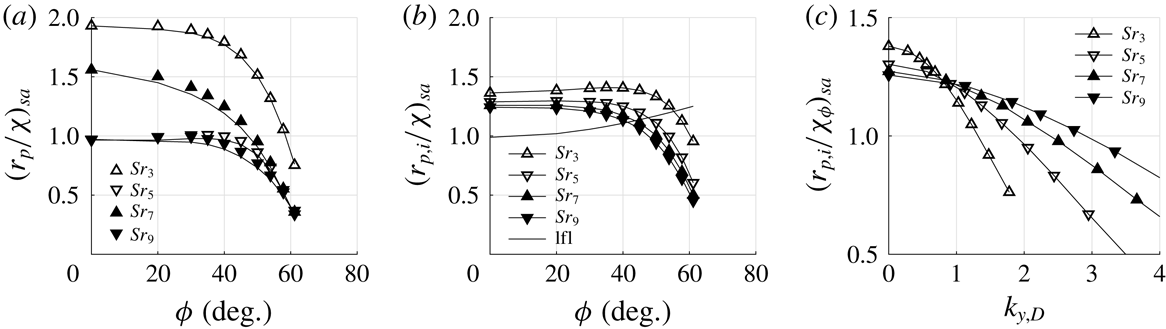
are compared to the data of continuous axisymmetric acoustic waves in figure 11(a). The data clearly match qualitatively but slight quantitative deviations are evident. The relative deviation increases with Strouhal number from
 $1.7$
to
 $7\,\%$
. An explanation can be found in the linear theory of shock–acoustic-wave interaction by McKenzie & Westphal (Reference McKenzie and Westphal1968). The shock is assumed to be continuously oscillating which gives a relative speed between shock and flow in the computation of wave transmission and reflection. In the present simulations, the shock is initially stationary and needs to be accelerated during transmission and reflection. The higher the Strouhal number, the higher is the shock velocity and its acceleration, which agrees with the trend in deviation with Strouhal number. Despite the slight discrepancy, the superposition of the pulse response satisfactorily represents the transfer function and will be further analysed to decompose
 $r_{p}$
into its contributions.
Transfer function
 $r_{p}$
: (a) comparison of
 $r_{p}$
reconstructed from the pulse response (symbol) and the data of continuous axisymmetric acoustic waves (line); (b) amplitude of the initially diverging acoustic wave at the stagnation point
 $r_{p,i}=\max (|r_{p}(t)|)$
, the low frequency limit from (2.14) is shown as ‘lfl’; (c) amplitude of the initially diverging acoustic wave scaled by the low frequency limit for inclined waves as a function of the radial wavenumber.

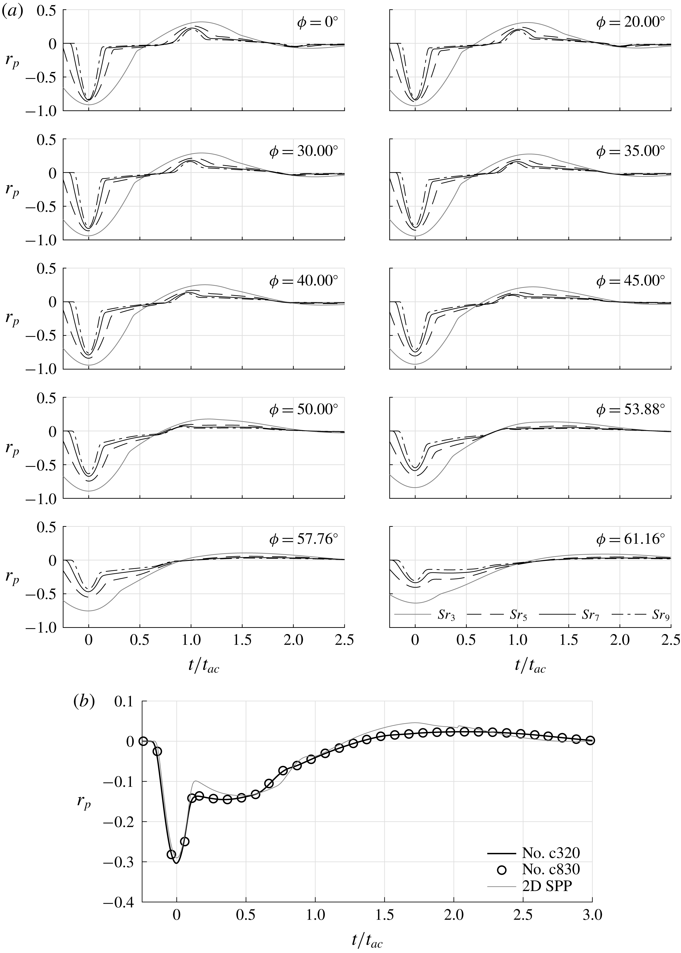
Time series of
 $r_{p}(t/t_{ac})$
of all pulse simulations are summarised in figure 12(a). The most intense fluctuation arises when the initially diverging acoustic wave is reflected. This incident is defined to occur at
 $t/t_{ac}=0$
and the corresponding absolute value
 $r_{p,i}$
is depicted in figure 11(b). Furthermore, the low frequency limit (2.14) is included. This comparison is valid since the low frequency limit denotes quasi-steady deviations from the unperturbed state. Therefore, a sinusoidal pulse with
 $Sr\rightarrow 0$
in the free stream translates directly into a sinusoidal response at the stagnation point. All remaining effects after the initial pulse in figure 12(a), e.g. the second pulse due to the shock reflected acoustic wave at
 $t/t_{ac}\approx 1$
, happen immediately compared to the period of the
 $Sr\rightarrow 0$
acoustic wave since
 $t_{ac}$
is constant and the period of the incident wave tends towards infinity. This is visualised in figure 12(a) by the vanishing separation of the initial pulse and the reflected pulse at
 $t/t_{ac}\approx 1$
as the Strouhal number decreases. For acoustic waves at
 $Sr\rightarrow 0$
, the pulse response consists only of the initial pulse and the frequency response collapses with the amplitude of the pulse response. With increasing Strouhal number, the initial pulse and following effects separate and the initial amplitude
 $r_{p,i}$
evolves from the low frequency limit to the DNS data. For the cases of figure 11(b), the separation is evident from figure 12(a).
Time traces of pressure fluctuations caused by pulses of inclined slow acoustic waves at the stagnation point: (a) the angle on incidence increases from top left to bottom right; (b) detailed view of the highest Strouhal number data
 $Sr_{9}=2.538$
from
 $\unicode[STIX]{x1D719}=61.16^{\circ }$
of (a), the symbols denote a validation simulation using a finer grid having
 $830$
cells on the axis of rotation between shock and stagnation point, ‘2D SPP’ denotes the two-dimensional configuration of the probe with an incident pulse at identical inclination angle and
 $Sr/Sr_{ac}$
.

For all inclination angles
 $\unicode[STIX]{x1D719}$
, the initial amplitude decreases with increasing Strouhal number and seems to converge to be Strouhal number independent. The focusing effect acts most intense at the lowest Strouhal number and with increasing Strouhal number, the linear interaction theory becomes more relevant and thus, the Strouhal number dependence vanishes. In the investigated range, complete Strouhal number independence is not reached. Like in the low frequency limit, the two lower Strouhal number cases in figure 11(b) show an initially slight increase of
 $r_{p,i}$
with inclination angle. Compared to the low frequently limit, the DNS
 $r_{p,i}$
are higher at low to moderate inclination angles and lower at high inclination angles. Towards
 $\unicode[STIX]{x1D719}=61.16^{\circ }$
, the initial amplitude rapidly decreases causing the
 $r_{p}$
trend of the continuous data in figure 9(a), i.e. the first transmission of the pulse through the shock wave accounts for the decay of
 $r_{p,i}$
at inclination angle. To analyse this decay, the three-dimensional flow has to be considered.
Whenever an incident plane pulse is transmitted by a curved bow shock, there is a point of normal incidence, e.g. for an axisymmetric flow field and a non-inclined incident wave this point coincides with the rotation axis. With increasing inclination angle, the interaction takes place further off the rotation axis with weaker portions of the curved bow shock. With decreasing shock strength, the transmission coefficient also decreases (McKenzie & Westphal Reference McKenzie and Westphal1968). For the present configuration, an inclination angle of
 $\unicode[STIX]{x1D719}=23.57^{\circ }$
leads to the normal incidence at approximately
 $y/R=0.85$
. This location defines the limit between postshock sub- and supersonic flow. For higher inclination angles, the interaction with the shock wave upstream of the subsonic part of the flow field always occurs at an incidence which is also known to influence the transmission coefficient (McKenzie & Westphal Reference McKenzie and Westphal1968). Furthermore, the path and development of the transmitted acoustic wave towards the stagnation point in the non-uniform postshock flow field are not trivial to determine, i.e. the relevant region of shock–acoustic-wave interaction defining the initial amplitude
 $r_{p,i}$
is hard to compute. Moreover, the circumferentially averaged transfer functions prevent the analysis off the rotation axis. Therefore, a definite rigorous explanation for the decay of
 $r_{p,i}$
cannot be given, yet.
(a) Initial pulse amplitude of the transfer function
 $r_{p,i}$
scaled by the low frequency limit of inclined waves
 $\unicode[STIX]{x1D712}_{\unicode[STIX]{x1D719}}$
versus the radial wavenumber
 $k_{y,D}$
scaled by
 $1+Sr/Sr_{ac}$
; (b) relative change between
 $r_{p}$
and
 $r_{p,i}$
due to pulse response superposition.

To define a criterion for the type of detection of an incident wave, i.e. initial amplitudes
 $r_{p,i}$
being higher or lower than the low frequency limit, the data of figure 11(b) are further analysed. The intersection of the DNS data with the low frequency limit shifts to lower angles with increasing Strouhal number and can be interpreted as the onset of the decay of
 $r_{p,i}$
. The initial amplitude scaled by the low frequency limit of inclined waves
 $\unicode[STIX]{x1D712}_{\unicode[STIX]{x1D719}}$
of (2.14) as a function of the radial wavenumber
 $k_{y,D}$
is analysed in figure 11(c). All transfer functions intersect in a narrow region at
 $k_{y,D}\approx 0.9$
. This value is more conservative compared to the intersection with the low frequency limit in figure 11(b), i.e. these points of intersection can be found at
 $r_{p,i}/\unicode[STIX]{x1D712}_{\unicode[STIX]{x1D719}}=1$
for
 $k_{y,D}>0.9$
in figure 11(c). The equidistant spacing starting at
 $k_{y,D}=1$
of these points suggests a Strouhal number based scaling as shown in figure 13(a). The intersection of the initial amplitude
 $r_{p,i}$
with the low frequency limit occurs when
 $k_{y,D}=1+Sr/Sr_{ac}$
. Given the fact that
 $Sr_{ac}$
can be estimated from the shock standoff distance and the postshock speed of sound, the empirical formula can be directly evaluated. It can easily be validated from figures 3 and 9(a) that both criteria from figures 11(c) and 13(a) work at the inclination angle of radiated waves.
The second suggested scaling of the radial wavenumber implies further information. First, it is evident that with increasing
 $Sr_{ac}$
the intersection with the low frequency limit shifts to higher Strouhal numbers and tends towards the first criterion. Moreover, a physical interpretation of the mutual point in figure 13(a) can be deduced by reformulating it
 $$\begin{eqnarray}Sr(1/Sr_{y}-1/Sr_{ac})=1,\end{eqnarray}$$
using (2.8) and the Strouhal number
 $Sr_{y}=D/(t_{y}u_{\infty })$
. The quantity
 $t_{y}$
denotes the duration of an incident wave to pass the probe radially
 $t_{y}=Dk_{y}/\unicode[STIX]{x1D714}$
. For
 $1/Sr_{y}\leqslant 1/Sr_{ac}$
, (5.3) can never be satisfied, and thus
 $1/Sr_{y}=1/Sr_{ac}$
represents the upper border of inclination angles with
 $r_{p,i}/\unicode[STIX]{x1D712}_{\unicode[STIX]{x1D719}}\geqslant 1$
. Since the radial phase velocity
 $\unicode[STIX]{x1D714}/k_{y}$
in
 $t_{y}$
only depends on the inclination angle of the incident wave, a limiting angle defines this border. The corresponding angle of incidence
 $\unicode[STIX]{x1D719}_{\star }$
follows from
 $$\begin{eqnarray}\unicode[STIX]{x1D719}_{\star }=\cos ^{-1}\left(\frac{1}{Ma\sqrt{Sr_{ac}^{2}+1}}\right)-\tan ^{-1}(Sr_{ac}).\end{eqnarray}$$
It is
 $\unicode[STIX]{x1D719}_{\star }=32.22^{\circ }$
for the current configuration. Relying on (5.3), for angles of incidence
 $\unicode[STIX]{x1D719}\leqslant \unicode[STIX]{x1D719}_{\star }$
, the abrupt decay of the transfer function cannot be expected. For the physical interpretation of
 $1/Sr_{y}=1/Sr_{ac}$
, the inverse Strouhal number is interpreted as a non-dimensional time. Under these conditions, the incident wave requires
 $t_{ac}$
to pass the SPP.
Furthermore, the transfer function
 $r_{p}$
is affected by resonance. Subsequent pulses interfere with the fluctuations following the initial pulse evident in figure 12(a). In general, the peak fluctuation of the superposed pulse responses does not necessarily occur exactly when the initial wave is reflected. Given the dominant fluctuation level of the initial pulse, the peak fluctuation of the superposed pulse responses can be found in the immediate vicinity. Therefore, the effect of resonance is quantified as the relative difference between the reconstructed transfer function
 $r_{p}$
and the initial pulse amplitude
 $r_{p,i}$
. The distribution of the effect of interference is shown in figure 13(b). Values
 ${<}0$
denote destructive interference, whereas values
 ${>}0$
mean resonant amplification. In addition to the highest initial peak amplitude, the lowest Strouhal number also shows by far the most intense resonant amplification. At
 $\unicode[STIX]{x1D719}=0^{\circ }$
, the remaining cases do not differ significantly showing values of approximately
 $\pm 0.25$
. Starting from the non-inclined cases at
 $\unicode[STIX]{x1D719}=0^{\circ }$
, the destructive and constructive interference decrease towards zero below
 $\unicode[STIX]{x1D719}=40^{\circ }$
but the initial type of interference is maintained, i.e. constructive or destructive. The decay of interference is more intense for constructive interference at
 $Sr_{3}$
and
 $Sr_{7}$
. In § 2.2, it was argued that, due to the inclination of the postshock wave, the postshock axial wavenumber distribution changes and modifies the phase difference of the superposing waves. This effect can be verified by comparing the time series of stagnation point pressure in figure 12(a) from
 $\unicode[STIX]{x1D719}=0^{\circ }$
to
 $\unicode[STIX]{x1D719}=45^{\circ }$
. The second peak at
 $t/t_{ac}$
shifts towards lower times, i.e. lower axial wavenumbers as the phase speed increases. This result agrees with the illustration of analytic isolines of constant axial wavenumber in figure 3. At higher inclination angles between
 $45^{\circ }$
and
 $50^{\circ }$
the
 $Sr_{7}$
data change the type of interference in figure 13(b). Discussing the effect of the postshock axial wavenumber in § 2.2, a change of type of interference was predicted by the same mechanism as the initial decay of interference of any type. On the contrary, none of the destructive cases
 $Sr_{5}$
and
 $Sr_{9}$
shows constructive interference. Therefore, the significance of the postshock axial wavenumber in the wavenumber map is limited to the prediction of the insensitivity of the resonant behaviour towards changes of the inclination angle at low inclination angles.
With increasing inclination angle, another effect supersedes the shift of the second peak in figure 12(a) and the simple underlying model of oscillating plane waves does not capture the resonant behaviour at high inclination angles. The time series in figure 12(a) show a plateau of the pressure fluctuations after the initial pulse. The end of the plateau hardly depends on the Strouhal number, but introduces a new time scale causing resonance. Since the new plateau follows the initial pulse with identical sign, the interference with the following pulse, i.e.
 $[\unicode[STIX]{x03C0},2\unicode[STIX]{x03C0}]$
, is of destructive type. The most prominent case of the investigation at the highest Strouhal number and inclination angle is highlighted in figure 12(b). The symbols represent a validation simulation using a much finer grid. The Strouhal number is high enough to have another pulse, i.e.
 $[2\unicode[STIX]{x03C0},3\unicode[STIX]{x03C0}/2]$
, which interferes with the pressure fluctuations at approximately
 $t/t_{ac}=0.5$
. Therefore, the destructive interference is weakened and the corresponding case in figure 13(b)
 $Sr_{9}$
does not gain destructive interference. The overall effect of this amplification is small. This can be seen in figure 8(a) by the slight increase of the inclined transfer function at higher Strouhal numbers and in figure 9(a) by the approach of the
 $Sr_{9}$
data towards the
 $Sr_{7}$
data.
To determine the mechanism of the new type of interference, the axisymmetric ansatz suffers from the disadvantage of a circumferentially integrated perturbation field. However, the two-dimensional configuration of the SPP shows very similar results. Although the transfer function
 $r_{p}$
is not identical comparing the two and three-dimensional configurations especially at low angles of inclination, the resonant behaviour can be essentially reproduced. In figure 12(b), also the pulse response of the two-dimensional simulation at identical inclination angle and
 $Sr/Sr_{ac}$
is shown to substantiate the following explanation. The new type of interference originates from two types of waves downstream of the shock wave occurring at high inclination angles, i.e. low radial phase velocities
 $\unicode[STIX]{x1D714}/k_{y}$
. First, there is the fast initially diverging acoustic wave causing the initial pulse during the reflection while propagating past the probe surface. Second, a slower non-acoustic pressure disturbance follows the initial pulse over the SPP causing the aforementioned plateau in figure 12(b).
The change of detection of an incident pulse by the probe determining the resonant behaviour is further illustrated in figure 14(a)–(d) by lines of constant
 $r_{p}$
drawn in a plane spanned by the time and rotation axis
 $(t/t_{ac},x/D)$
for several inclination angles at the highest Strouhal number. The contour levels are in per cent of
 $r_{p,i}$
, dash-dotted lines denote negative and solid lines positive values. In figure 14(a), the non-inclined transmitted pulse propagates from the lower left towards the stagnation point at
 $(0,0)$
and reflects back and forth between probe and shock wave. The focusing effect is evident as the transfer function increases towards the stagnation point. The second peak is, as predicted by
 $t_{ac}$
, at
 $(1,0)$
. At
 $\unicode[STIX]{x1D719}=45^{\circ }$
in figure 14(b), the low inclination detection of the incident pulse is still evident. As aforementioned and shown in figure 12(a), the decreasing axial wavenumber causes the period between reflections at the stagnation point to decrease in figure 14(b). The focusing effect is absent for the initially diverging acoustic wave but acts on the first shock reflected wave. The phase shift, i.e. the change of sign, at the shock wave is apparent for both angles of inclination.
Lines of constant transfer function
 $r_{p}$
: (a)–(d) show time and rotation axis plane; the transfer function is scaled by the absolute value of the extremum at the stagnation point
 $r_{p}/r_{p,i}$
and is given in %; dash-dotted lines denote negative and solid lines positive values; (e) lines of constant transfer function of the two-dimensional configuration at
 $\unicode[STIX]{x1D719}=61.16^{\circ }$
, the plane is spanned by the time and the coordinate along the flat surface of the probe, the dashed line denotes a phase speed of
 $1.25a_{0}$
and the dash-dotted line represents the radial phase speed
 $\unicode[STIX]{x1D714}/k_{y}$
of the incident wave.

For the inclination angle
 $\unicode[STIX]{x1D719}=53.88^{\circ }$
in figure 14(c), the explicit wave pattern is disturbed. The initially diverging acoustic wave and its reflected acoustic wave still show the back and forth behaviour at lower axial wavenumbers. However, the shock reflected wave is only indicated by the isolines of
 $-8$
and
 $1$
in the range
 $0.5<t/t_{ac}<1.5$
. The wave passing the stagnation point at
 $(1.5,0)$
is much clearer illustrated. This is the shock reflected wave of the wave reflected from the rounded corner of the SPP. The interaction happens at a low angle of incident further off the rotation axis and therefore, the model in § 2.2 based on the postshock axial wavenumber cannot explain the temporal development of the wave. At
 $\unicode[STIX]{x1D719}=61.16^{\circ }$
in figure 14(d), the initially diverging wave propagates perpendicular to the rotation axis. Since
 $\unicode[STIX]{x1D719}$
exceeds
 $\unicode[STIX]{x1D719}_{\dagger }$
on the rotation axis, an evanescent wave passes downstream of the shock wave at
 $t/t_{ac}=0$
. Then, the transmitted wave reflected from the probe interacts with the shock wave. From the isoline with the value
 $-70$
emanating from
 $(0,0)$
, a value of
 $t/t_{ac}=0.3$
can be determined. The wave pattern still follows the theory from § 2.2, but the shock reflected wave is insignificant. At times
 $t/t_{ac}>1.3$
, the acoustic wave caused by the rounded corner appears. The newly occurring pressure wave is located in the vicinity of
 $(0.3,0)$
. When the initial wave outruns the evanescent wave at she shock and the new pressure wave at the SPP, the latter two jointly propagate.
To further analyse the new pressure wave using the aforementioned two-dimensional SPP configuration, the wave speed is determined by lines of constant pressure fluctuations in the plane spanned by the time and the
 $y$
coordinate parallel to the probe surface in figure 14(e). The wave front approximated by the dashed line represents the reflection of the initially diverging fast acoustic wave. From the slope of the dashed line, its phase speed
 $1.25a_{0}$
can be estimated. The new pressure wave follows the acoustic wave at lower phase velocity. The slope of the dash-dotted line is determined by the radial phase velocity
 $\unicode[STIX]{x1D714}/k_{y}=0.747$
imposed by the free stream disturbance and shows agreement with the spatial evolution of the pressure wave which is too slow for an acoustic wave. Furthermore, when the acoustic wave reduces its amplitude, the pressure wave gains strength. The mechanism causing the non-acoustic pressure wave remains unclear. On the one hand, the wave could be generated during the reflection of the acoustic wave in the non-uniform flow field downstream of the shock wave. In this scenario, the agreement of the radial phase velocity with the evanescent wave seems arbitrary since the acoustic wave gained phase speed before its reflection. On the other hand, the pressure wave might constitute a direct consequence of the postshock evanescent wave that was predicted to occur at angles
 ${>}\unicode[STIX]{x1D719}_{\dagger }$
in § 2.2 and observed in the analysis of figure 14(d). It also constitutes a non-acoustic pressure wave and propagates with the radial phase velocity of the incident wave. At any rate, the wave is imposed by the free stream disturbance and poses an additional source for interference at high angles of inclination.
6 Conclusion
The calibration in form of a transfer function
 $r_{p}$
relating stagnation point pressure fluctuations of SPPs to inclined slow acoustic waves in the free stream, which are, e.g. radiated by turbulent supersonic boundary layers, is conducted by DNS. To lower the computational effort, a new formulation for boundary conditions is derived to reduce the three-dimensional flow to an axisymmetric problem.
Using numerical data from Duan & Choudhari (Reference Duan and Choudhari2013) and experiments by Laufer (Reference Laufer1961), the inclination angle of acoustic waves radiated by a turbulent supersonic boundary layer is determined
 $\unicode[STIX]{x1D719}=61.16^{\circ }$
. An analytical low frequency limit
 $\unicode[STIX]{x1D712}_{\unicode[STIX]{x1D719}}(\unicode[STIX]{x1D719})$
for
 $r_{p}$
is derived from a high Mach number formulation of the Rayleigh Pitot-tube formula.
Then, DNS of the flow around a cylindrical SPP with a rounded edge are presented. The transfer function
 $r_{p}$
as a function of the Strouhal number for the inclination of the radiated waves exceeds its low frequency limit at low Strouhal numbers. However, at approximately
 $Sr=0.5$
, the transfer function decreases abruptly. The comparison to numerical data of Duan et al. (Reference Duan, Choudhari, Chou, Muñoz, Ali, Radespiel, Schilden, Schröder, Marineau and Casper2018) for a different blunt configuration shows good agreement and suggests the normalisation proposed by Chaudhry & Candler (Reference Chaudhry and Candler2017) to hold at high inclination angles. The effect of wave inclination is also defined by a sudden steep decrease of the transfer function towards high inclination angles.
Four important implications considering the measurement of tunnel noise are made. First, the wide range of the transfer function
 $r_{p}$
necessitates experimental data in the form of power spectral density (PSD) distributions or bandwidth filtered nRMS values to accurately account for the frequency dependence. Second, broad bandwidth filtered data in the range of
 $Sr=0.5$
should be avoided. Third, since the transfer functions of non-inclined fast acoustic waves and slow acoustic waves at radiation inclination differ by one order of magnitude at high Strouhal numbers, the choice of transfer function for the calibration has to be thoroughly considered. Fourth, the propagation of uncertainty in the inclination angle of the radiated waves, that are to be measured, has a pronounced impact on the resulting free stream pressure amplitude. The choice of the inclination angle to determine the transfer function
 $r_{p}$
is extremely important and should carefully be considered to estimate the error of the calibration of the SPP. Altogether, to accurately determine tunnel noise, the type and order of magnitude of the disturbances present in the free stream have to be known a priori to choose an appropriate method and select adequate transfer functions. Therefore, the idea of the existence of an all-embracing transfer function for SPPs must be questioned rendering tunnel noise measurements a very delicate subject.
Considering the severe decay of the transfer function for inclination angles of radiated waves and the decrease for increasing angle of incidence, the relation
 $k_{y,D}=1+Sr/Sr_{ac}$
is found to describe its onset. The criterion yields a limiting angle
 $\unicode[STIX]{x1D719}_{\star }$
. For inclination angles less than
 $\unicode[STIX]{x1D719}_{\star }$
, no decay of the transfer function can be expected.
The impact of averaging is investigated first for a PCB pressure transducer. The effect is not negligible but not massive, i.e. the distribution of the stagnation point data is maintained. Averaging over the complete flat surface of the probe causes a severe decay of the transfer function to very low values. The onset of intense cancellation collapses for the radial wavenumber of
 $k_{y,D}=2$
with the wavenumber of the flat surface being
 $1.84$
.
Finally, the influence of resonance is analysed. The behaviour at low angles of inclination is dominated by postshock oscillating waves. For radiation inclination, destructive interference dominates at all four Strouhal numbers caused by a pressure wave occurring at the probe surface. The shock reflected wave which is responsible for the resonant behaviour at low inclination angles diminishes. The new time scale introduced by the pressure wave mainly depends on the inclination angle. In accordance with this observation, the radial phase speed of the incident wave
 $\unicode[STIX]{x1D714}/k_{y}$
, which is only a function of the inclination angle, agrees with the speed of the pressure wave along the probe surface.
The current results shed light on the application of SPPs for tunnel noise measurements in supersonic testing facilities by discussing transfer functions, error approximations and mechanisms.
Acknowledgements
This work has been funded by the German Research Foundation (DFG) within the HYPTRANS PAK742. The support is gratefully acknowledged. Computing resources were provided by the High Performance Computing Centre Stuttgart (HLRS) and the Jülich Supercomputing Centre.