1. Introduction
The dynamics of hydraulic fracturing is a particularly interesting problem and has attracted significant research attention during the past several decades (e.g. Spence & Sharp Reference Spence and Sharp1985; Lister Reference Lister1990a ; Savitski & Detournay Reference Savitski and Detournay2002; Lai et al. Reference Lai, Zheng, Dressaire, Wexler and Stone2015; OKeeffe & Linden Reference OKeeffe and Linden2017). There has been significant interest during the past decade to explore unconventional fluid-phase resources such as shale gas and tight oil in industry, and this technology is crucial to fracture porous rocks to create more permeable pathways for gas and oil to flow (e.g. Bickle et al. Reference Bickle, Goodman, Mair, Roberts, Selley, Shipton, Thomas and Younger2012; Patzek et al. Reference Patzek, Male and Marder2013; Cueto-Felgueroso & Juanes Reference Cueto-Felgueroso and Juanes2013). A closely related environmental issue is that once pressure is released after an initial period of fracturing, the injected fluid flows back, driven by elastic stresses, carrying possibly pollutants and chemicals up to the drinking water layers and the ground surface (e.g. Bickle et al. Reference Bickle, Goodman, Mair, Roberts, Selley, Shipton, Thomas and Younger2012; Lai et al. Reference Lai, Zheng, Dressaire, Ramon, Huppert and Stone2016a ). The influence of seismic waves, generated during subsurface injection activities, also draws concerns (e.g. Schultz et al. Reference Schultz, Atkinson, Eaton, Gu and Kao2018). Also, in geophysical contexts, for several decades, the theory of hydraulic fracturing has been applied to explain the formation of magma-driven dykes and laccoliths (e.g. Lister & Kerr Reference Lister and Kerr1991; Rubin Reference Rubin1995), the migration of the tidal grounding line between ice sheets and bedrocks (e.g. Warburton Reference Warburton2020) and the drainage of glacier lakes underneath ice sheets in polar regions (e.g. Rice et al. Reference Rice, Tsai, Fernandes and Platt2015; Lai et al. Reference Lai, Stevens, Chase, Creyts, Behn, Das and Stone2021). All of these applications provide additional motivations to understand the fundamentals of the coupled process of fluid flow and material deformation.
Many previous studies were dedicated to understand the dynamics of hydraulic fracturing in elastic solids, including theoretical (e.g. Spence & Sharp Reference Spence and Sharp1985; Lister Reference Lister1990a ; Savitski & Detournay Reference Savitski and Detournay2002), experimental (e.g. Lai et al. Reference Lai, Zheng, Dressaire, Wexler and Stone2015; OKeeffe & Linden Reference OKeeffe and Linden2017), numerical efforts and a combination of them. These studies typically focused on the model problem of hydraulic fracturing in infinite elastic and brittle materials. The influence of viscous flow, elastic deformation and material breaking at a frature’s tip (in the form of material toughness) were clarified gradually. Detailed asymptotic structures were also obtained by solving a boundary value problem of a nonlinear non-local ordinary differential system to describe a fracture’s profile shape at the self-similar stage and the pressure distribution within the fluid film (e.g. Spence & Sharp Reference Spence and Sharp1985; Lister Reference Lister1990a ; Savitski & Detournay Reference Savitski and Detournay2002). Scaling analyses are also found to be particularly useful to quickly estimate typical values and the parametric dependence of a fracture’s length and thickness evolution and the fluid pressure within a fracture. The predictions were often found to compare favourably with laboratory experimental data of hydraulic fracturing in transparent elastic solids such as gelatins (e.g. Lai et al. Reference Lai, Zheng, Dressaire, Wexler and Stone2015,Reference Lai, Zheng, Dressaire and Stone2016b ; Tanikella & Dressaire Reference Tanikella and Dressaire2022) and hydrogels (e.g. OKeeffe & Linden Reference OKeeffe and Linden2017; OKeeffe et al. Reference OKeeffe, Huppert and Linden2018), or in-between two thick layers of polymethyl methacrylate (PMMA) /glass blocks that are cemented together (e.g. Bunger & Detournay Reference Bunger and Detournay2008).
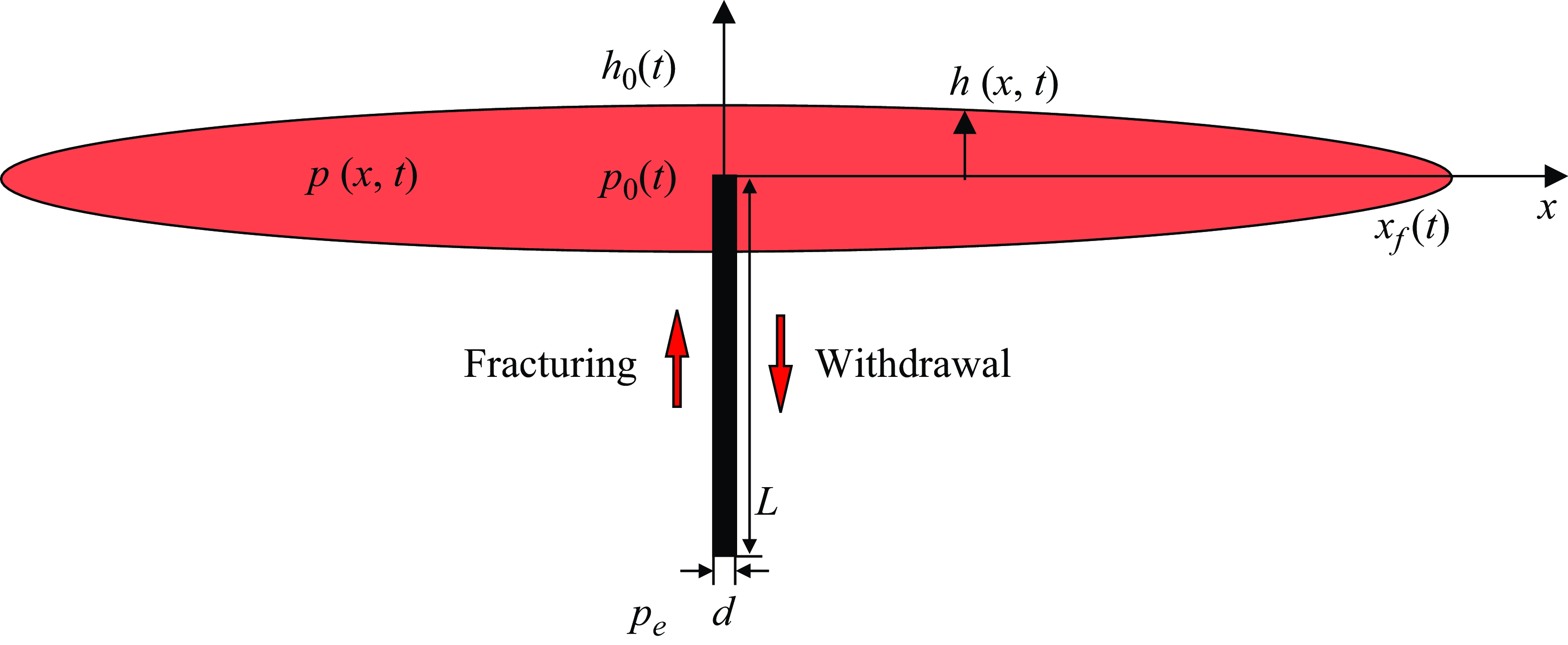
Sketch of a deflating fracture subject to fluid withdrawal through a narrow conduit of width
 $d$
and length
 $L$
located at the centre
 $(x=0)$
. The profile shape is denoted by
 $h(x,t)$
and the pressure distribution is denoted by
 $p(x,t)$
within a fracture. The front of the fluid film locates at
 $x=x_f(t)$
, which is also the tip of the fracture here. The rate of fluid injection/withdrawal depends on the pressure difference
 $\triangle p \equiv p_0(t) - p_e$
between the inlet and outlet of the conduit.

The current work focuses on the viscous backflow process during fracture deflation once pressure is released, as shown in figure 1, which is much less studied. Upon pressure release at the outlet of the conduit, the fracturing fluid flows out of the elastic solid through the narrow conduit, and the fracture deflates. In a previous work (Zheng Reference Zheng2024b ), we considered the viscous regime when the influence of material toughness is negligibly small. We found that with fluid extraction the fracture’s thickness at the location of the conduit approaches zero as fluid removal proceeds, while the fracture’s front continues to propagate. As time progresses, the dipole moment becomes conserved eventually for this system of coupled flow and deformation. A self-similar solution of the dipole type can also be obtained to describe the universal dynamics for the coupled evolution of the profile shape and the pressure distribution within the fluid film at intermediate times. Here, we further consider the influence of the material toughness on the dynamics of fracture deflation when the elastic solid is also brittle. We demonstrate that the theory presented here is consistent with previous experimental observations of backflows from transparent solid gelatins with fixed frontal locations (e.g. Lai et al. Reference Lai, Zheng, Dressaire, Ramon, Huppert and Stone2016a ).
This paper is structured as follows. In § 2 we first present a theoretical model that considers thin film flow, elastic deformation and material breaking at the tip. The novel ingredients are to couple the description of fluid removal through a narrow conduit at the centre, and to consider appropriately the propagation condition at the fracture’s front. In § 3 we then describe the behaviours at two limiting regimes that exhibit dipole-flow and fixed-length dynamics, respectively, with fluid extraction, and in both regimes, self-similar solutions can be obtained to describe the universal behaviours at intermediate times. We then explore a special situation of purely elasticity-driven fracture deflation without suction and obtain a different set of self-similar solutions to describe intermediate behaviours now with the zero pressure at the conduit. Comparison between theoretical predictions and available experimental observations is then briefly discussed for the evolution of the profile shape and fluid volume. In § 4 we conclude the paper with a brief summary and final remarks on potential implications.
2. Theoretical model
2.1. Governing equations
It is well documented (e.g. Spence & Sharp Reference Spence and Sharp1985) that, during hydraulic fracturing of an infinite elastic solid (see figure 1), time evolution of the profile shape
 $h(x,t)$
and pressure distribution
 $p(x,t)$
within the fluid film can be described by a coupled partial differential–integral system:
 \begin{align} \frac {\partial h}{\partial t} - \frac {1}{3\mu }\frac {\partial }{\partial x}\left (h^3\frac {\partial p}{\partial x}\right ) = 0, \end{align}
 \begin{align} p(x,t) = -\frac {E}{2(1-\sigma ^2)} \frac {1}{\pi }\int _{-x_f(t)}^{x_f(t)} \frac {1}{s-x}\frac {\partial h}{\partial s}\textrm { d}s. \end{align}
Here
 $\mu$
denotes the viscosity of the fluid,
 $E$
and
 $\sigma$
denote the Young’s modulus and Poisson ratio of the elastic solid, respectively. Physically, (2.1a
) describes the lubricating thin film flow, while (2.1b
) describes the pressure evolution due to elastic deformation within the fluid film.
The influence of a constant far-field normal stress can also be considered based on the current model by defining appropriately a net pressure, which leads to the presence of a lag region ahead of the fluid front rather than allowing for the existence of a pressure singularity (e.g. Spence & Sharp Reference Spence and Sharp1985; Lister Reference Lister1990a ). We refer the interested reader to, e.g., Garagash (Reference Garagash2006) for detailed discussions. In the limit of the far-field compressive stress being infinite compared with the elastic pressure, the length of the lag region approaches zero and the overall dynamics approaches that of Spence & Sharp (Reference Spence and Sharp1985). We must also note that there is no clear evidence of a lag region being significantly developed in the experiments performed by Lai et al. (Reference Lai, Zheng, Dressaire, Wexler and Stone2015,Reference Lai, Zheng, Dressaire and Stone2016b ) and OKeeffe et al. (Reference OKeeffe, Huppert and Linden2018) for the parameter ranges considered. In these experiments, no external compressive stress was imposed but the weight of the elastic solids might be relevant.
Equations (2.1a , b ) must be solved subject to
 \begin{align} h(x,0) = 0, \end{align}
 \begin{align} h(\pm x_f(t),t) = 0, \end{align}
 \begin{align} \int _{-x_f(t)}^{x_f(t)} h(x,t)\, {\textrm {d}}x = 2qt. \end{align}
Furthermore, note that
 $x_f(0) = 0$
for the initial frontal location. Initial condition (2.2a
) indicates that there exists no fluid within the elastic solid before fracturing, boundary condition (2.2b
) indicates that there exists a couple of propagating fronts (i.e. fracture tips) at
 $x = \pm x_f(t)$
, and the global volume constraint (2.2c
) indicates that the total fluid volume within a fracture increases linearly and is proportional to the area rate of injection
 $q$
in the positive/negative half-domain of the two-dimensional configuration. It is also convenient to modify condition (2.2c
) to describe hydraulic fracturing under a time-dependent injection rate
 $q(t)$
. The integral condition (2.2c
) can also be modified appropriately to provide a flux boundary condition at the location of the conduit
 $x=0$
as
 $-(3\mu )^{-1}\, h^3 \partial p/\partial x|_{x=0} = q$
, knowing that the flux at the front
 $x=x_f(t)$
is zero. This is more convenient to apply in finite volume schemes to solve (2.1a
,
b
) subject to initial and boundary conditions (IBCs) (2.2a
–
c). A similar treatment has been employed previously to study the injection regimes of a gravity current into a confined porous layer, which leads similarly to the flux condition (2.10) at the source in Zheng et al. (Reference Zheng, Guo, Christov, Celia and Stone2015).
When fluid withdrawal is allowed through a narrow conduit of width
 $d$
and length
 $L$
at the centre
 $(x=0)$
, as sketched in figure 1, a fracture deflates gradually as fluid removal continues, driven by the pressure difference between the inlet and outlet of the conduit. For the one-dimensional viscous flow within the conduit, the rate of fluid removal is given by
 \begin{equation} q_0(t) = \frac {d^3}{12 \mu } \frac {p_0(t)-p_e}{L}, \end{equation}
where
 $p_0(t)$
and
 $p_e$
denote the pressure at the inlet and outlet of the conduit, respectively, in the two-dimensional configuration. It is important to note that the elastic pressure
 $p_0(t)$
depends on the deformation evolution
 $h(x,t)$
of the elastic solid, which is coupled with the elasto-hydrodynamic description (2.1a
,
b
) at any particular time of interest. This flux condition could be appropriately integrated into the description of (2.1a
,
b
) as a flux boundary condition at the centre, as described in an earlier work (Zheng Reference Zheng2024b
), when the influence of material toughness is negligibly small
 $(K_c=0)$
.
When an elastic solid is also brittle, on the basis of (2.1a
,
b
) with IBCs (2.2a
–c), the propagation of a hydraulic fracture must satisfy an additional propagation condition that is related to a material property named material toughness
 $K_c$
(e.g. Rice Reference Rice and Liebowitz1968; Lister Reference Lister1990a
):
 \begin{equation} K_I \equiv \frac {E}{2^{3/2}(1-\sigma ^2)}\frac {h}{(x_f-x)^{1/2}} = K_c,\,\,\,\mbox {as}\,\,\, x\to x_f^-. \end{equation}
Physically, (2.4) indicates that to break the material at the tip (for a crack to propagate), the fluid pressure (or, more precisely, the stress intensity factor
 $K_I$
) must be large enough to supply enough energy. This is an important feature of hydraulic fracturing in elastic and brittle materials (e.g. Spence et al. Reference Spence, Sharp and Turcotte1987; Lister Reference Lister1990b
; Savitski & Detournay Reference Savitski and Detournay2002), which could significantly impact the fracturing dynamics and makes it fundamentally different from the propagation of a viscous gravity current (e.g. Huppert Reference Huppert1982; Lister Reference Lister1992). The current work focuses particularly on the influence of material toughness
 $K_c$
on the dynamics of fracture deflation during fluid withdrawal.
2.2. Non-dimensionalisation
To be consistent with Zheng (Reference Zheng2024b
) in the viscous regime with
 $K_c=0$
, the model problem here is also non-dimensionalised based on the final state after an initial fracturing period of
 $t \in [0, t_i]$
. The characteristic time scale is chosen as
 $t_c = t_i$
, and the characteristic length, thickness and pressure scales are chosen based on that of a fracture at the end of the fracturing process. Following a scaling analysis of (2.1a
,
b
) subject to (2.2a–
c), the characteristic scales are chosen as
 \begin{align} x_c = t_i^{2/3} \left [\frac {Eq^3}{6\pi \mu (1-\sigma ^2)}\right ]^{1/6},\qquad h_c = t_i^{1/3}\left [\frac {6\pi \mu q^3(1-\sigma ^2)}{E}\right ]^{1/6},\\ \nonumber p_c = t_i^{-1/3}\left [\frac {3\mu E^2}{4\pi ^2(1-\sigma ^2)^2}\right ]^{1/3}. \end{align}
These results for the initial fracturing process are standard and consistent with those obtained by, e.g. Spence & Sharp (Reference Spence and Sharp1985); Detournay (Reference Detournay2004); and Garagash (Reference Garagash2006). These results are also analogous to standard scaling results for the growth of penny-shaped hydraulic fractures in elastic solids (e.g. Spence & Sharp Reference Spence and Sharp1985; Savitski & Detournay Reference Savitski and Detournay2002; Lai et al. Reference Lai, Zheng, Dressaire, Wexler and Stone2015; OKeeffe et al. Reference OKeeffe, Huppert and Linden2018). We then define dimensionless variables as
 $\bar {t} \equiv t/t_i$
,
 $\bar {x} \equiv x/x_c$
,
 $\bar {h} \equiv h/h_c$
,
 $\bar {p} \equiv p/p_c$
, and arrive at a dimensionless system for the initial period of hydraulic fracturing as
 \begin{align} \frac {\partial \bar {h}}{\partial \bar {t}} - \frac {\partial }{\partial \bar {x}}\left (\bar {h}^3\frac {\partial \bar {p}}{\partial \bar {x}}\right ) = 0, \end{align}
 \begin{align} \bar {p}(\bar {x},\bar {t}) = - \int _{-\bar {x}_f(\bar {t})}^{\bar {x}_f(\bar {t})} \frac {1}{s-\bar {x}}\frac {\partial \bar {h}}{\partial s}\textrm { d}s, \end{align}
subject to
 \begin{align} \bar {h}(\bar {x},0) = 0, \end{align}
 \begin{align} \bar {h}(\pm \bar {x}_f(\bar {t}),\bar {t}) = 0, \end{align}
 \begin{align} \int _{-\bar {x}_f(\bar {t})}^{\bar {x}_f(\bar {t})} \bar {h}(\bar {x},\bar {t})\, \textrm { d}\bar {x} = 2\bar {t}, \end{align}
for the time period of
 $\bar {t} \in [0,1]$
.
Since the problem is symmetric about the
 $z$
axis, it is convenient to consider only the positive half-domain, and in this case the elasticity equation (2.6b
) is rewritten as
 \begin{equation} \bar {p}(\bar {x},\bar {t}) = - \int _{0}^{\bar {x}_f(\bar {t})} \frac {2s}{s^2-\bar {x}^2}\frac {\partial \bar {h}}{\partial s}\textrm { d}s, \end{equation}
with the contribution of elastic deformation on the negative half-domain appropriately accounted for. Also, the global mass conservation equation (2.7c
) can be rewritten as a flux condition at
 $\bar {x}=0$
as
 \begin{equation} -\bar {h}^3\frac {\partial \bar {p}}{\partial \bar {x}}\bigg |_{\bar {x} = 0} = 1, \end{equation}
which is more convenient to impose in finite volume schemes to numerically solve the governing system of the evolution type (e.g. Zheng Reference Zheng2024a
). Similar treatment has been employed previously in analogous problems of fluid injection and gravity current spreading in porous layers (e.g. Zheng et al. Reference Zheng, Guo, Christov, Celia and Stone2015). For the initial fracturing process, we then solve the differential–integral system (2.6a
) and (2.9) subject to IBCs (2.7a
,
b
) and (2.9) for the time period of
 $\bar {t} = [0,1]$
to obtain the coupled time evolution of
 $\bar {h}(\bar {x}, \bar {t})$
and
 $\bar {p} (\bar {x}, \bar {t})$
.
For the backflow process after initial fracturing, meanwhile, the rate of fluid removal becomes
 \begin{equation} -\bar {h}^3\frac {\partial \bar {p}}{\partial \bar {x}} \bigg |_{\bar {x}=0} \equiv -\frac {1}{2}\bar {q}_0(\bar {t}) = - \Pi _c\, \bar {p}_0(\bar {t}) - \Pi _e, \end{equation}
where
 $\bar {q}_0 \equiv q_0/q$
and the two dimensionless parameters
 $\Pi _c$
and
 $\Pi _e$
are defined as
 \begin{equation} \Pi _c \equiv \frac {E^{2/3} d^3}{[48\pi \mu (1-\sigma ^2)]^{2/3}\,q L\, t_i^{1/3}} \quad \mbox {and}\quad \Pi _e \equiv -\frac {p_e d^3}{12\mu q L}. \end{equation}
Note that the flux condition (2.10) is written for the fracture evolution system (2.6a
,
b
), while the flow rate (2.3) is written for the viscous flow within the conduit. A positive flow rate in the conduit indicates fluid removal from the fracture, which is why we must include a negative sign in condition (2.10) for the fracture’s evolution. Note also that since we now consider only the positive half-domain, we use half the flow rate (2.3) in the conduit that could impact the backflow dynamics, which is why we include a prefactor of 1/2 for the second term in condition (2.10). The procedure is exactly the same as that of Zheng (Reference Zheng2024b
), where we arrived at exactly the same dimensionless parameters
 $\Pi _c$
and
 $\Pi _e$
. Physically,
 $\Pi _c$
measures the influence of elasticity-driven backflow compared with the thin film flow within a fracture, while
 $\Pi _e$
measures the influence of ambient-pressure-driven backflow (when
 $p_e \lt 0$
) compared with the thin film flow, i.e. the influence of external extraction (suction), when
 $\Pi _e \gt 0$
. The definition and physical meaning of
 $\Pi _c$
and
 $\Pi _e$
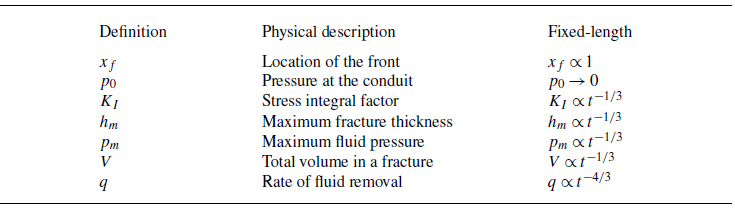
are included in table 1.
The three dimensionless parameters
 $\Pi _c$
,
 $\Pi _e$
,
 $\Pi _k$
for the process of viscous backflow and fracture deflation following hydraulic fracturing of an infinite elastic and brittle solid.

2.3. The influence of material toughness
The novel ingredient here, compared with Zheng (Reference Zheng2024b ), is the inclusion of the propagation condition (2.4), which can also be made dimensionless as
 \begin{equation} \bar {K}_I \equiv \frac {\bar {h}}{(\bar {x}_f-\bar {x})^{1/2}} = \Pi _k,\,\,\,\mbox {as}\,\,\, \bar {x} \to \bar {x}_f^-, \end{equation}
where the dimensionless material toughness
 $\Pi _k$
is defined as
 \begin{equation} \Pi _k \equiv \frac {2^{3/2}K_c(1-\sigma ^2)}{E}\frac {x_c^{1/2}}{h_c} = K_c\left [\frac {32(1-\sigma ^2)^3}{3\pi \mu qE^3}\right ]^{1/4}. \end{equation}
We also continue to use the same characteristic time, length and thickness scales of (2.5), obtained for the initial fracturing process. The definition and physical meaning of
 $\Pi _k$
are included also in table 1.
The focus of the current work is on the influence of the dimensionless material toughness
 $\Pi _k$
on the dynamics of flowback. Of particular interest is the toughness-dominated regime of
 $\Pi _k \gg 1$
, since the viscous regime (
 $\Pi _k = 0$
) has already been studied in Zheng (Reference Zheng2024b
). But before we move on with detailed numerical and analytical efforts, we briefly note that the influence of material toughness on the growth of hydraulic fractures has already been discussed in previous studies with (e.g. Spence et al. Reference Spence, Sharp and Turcotte1987; Lister Reference Lister1990a
,Reference Lister
b
; Roper & Lister Reference Roper and Lister2007) and without (e.g. Spence & Sharp Reference Spence and Sharp1985; Detournay Reference Detournay2004) the influence of buoyancy. In particular, in a neutrally buoyant environment, the influence of flow becomes negligible in the toughness-dominated regime when
 $\Pi _k \gg 1$
, as a fracture propagates in a quasi-steady fashion that always maintains an elliptic shape (e.g. Howell et al. Reference Howell, Kozyreff and Ockendon2008). There are also observations from laboratory experiments on the propagation dynamics of penny-shaped hydraulic fractures in blocks of elastic and brittle solids such as the transparent gelatins (e.g. Gelatin type A, ThermoFisher Scientific) and hydrogels (e.g. prepared from free radical polymerization of acrylamide monomer and cross-linker, Sigma Aldrich) (e.g. Lai et al. Reference Lai, Zheng, Dressaire, Wexler and Stone2015,Reference Lai, Zheng, Dressaire and Stone2016b
; OKeeffe & Linden Reference OKeeffe and Linden2017; OKeeffe et al. Reference OKeeffe, Huppert and Linden2018; Tanikella & Dressaire Reference Tanikella and Dressaire2022), along with analogous theoretical descriptions in the radial configuration (e.g. Spence & Sharp Reference Spence and Sharp1985; Savitski & Detournay Reference Savitski and Detournay2002).
Another type of experiments that was performed involved in two thick layers of transparent solid blocks (e.g. PMMA or borosilicate glass blocks) cemented together using a thin layer of transparent epoxy (e.g. Araldite K3600 of 0.01 mm in thickness) (e.g. Bunger & Detournay Reference Bunger and Detournay2008). The design of these experiments were more like the peeling-elastica experiments (e.g. McEwan & Taylor Reference McEwan and Taylor1966; Pihler-Puzovic et al. Reference Pihler-Puzovic, Illien, Heil and Juel2012), but with very thick elastic layers. The profile shapes measured in these experiments also appear to agree well with theoretical predictions of the same models in both the viscous and toughness regimes (e.g. Spence & Sharp Reference Spence and Sharp1985; Savitski & Detournay Reference Savitski and Detournay2002).
Representative numerical solutions showing the influence of
 $\Pi _k$
on the profile shape evolution with extraction (
 $\Pi _e \gt 0$
). We used the same
 $\{\Pi _c, \Pi _e\}$
in all subfigures (a, b, and c), the values of which do not influence the qualitative trend of the frontal dynamics during fracture deflation. The value of
 $\Pi _k$
impacts significantly the frontal dynamics and distinguishes the limiting regimes that exhibit dipole-flow and fixed-length behaviours in (a) and (c), respectively. We used 150–200 grids for these results for a sense of the numerical error.

2.4. Numerical observations
We then solve the dimensionless system of (2.6a
,
b
) subject to appropriate IBCs and propagation conditions for a rich set of fracture deflation phenomena during fluid withdrawal through a conduit. A finite volume scheme is employed, similar to those described in the appendices of Zheng (Reference Zheng2024a
,Reference Zhengb) on different but related problems of hydraulic fracturing, and we do not repeat the descriptions here. The initial condition is imposed in a consistent way, taken as the final state after an initial fracturing period of
 $\bar {t} \in [0,1]$
. In all cases, it is also ensured that the constraint
 $\bar {h}(\bar {x}, \bar {t}) \geqslant 0$
is imposed in the scheme for the profile thickness throughout the time evolution. This is particularly relevant at the source when
 $\Pi _e \gt 0$
, without which possibly negative and unphysical values of
 $\bar {h}(0, \bar {t}) \geqslant 0$
would result from imposing the extraction condition (2.10), similar to the analogous problem of gravity current extraction at a point source (e.g. Dudfield & Woods Reference Dudfield and Woods2012,Reference Dudfield and Woods2014). The dynamics is under the influence of three dimensionless parameters
 $\{\Pi _c, \Pi _e, \Pi _k\}$
.
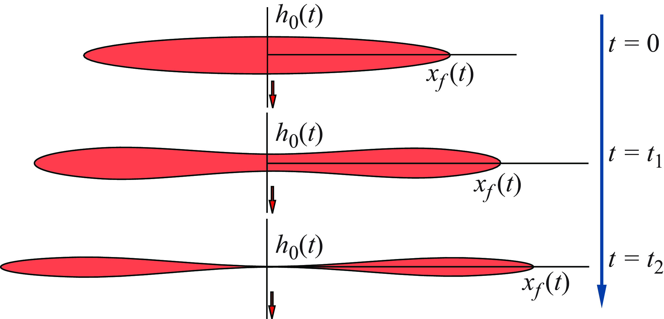
Here we present representative solutions for the profile shape evolution, as shown in figure 2, imposing appropriate values of the dimensionless control parameters. These numerical solutions shed light on two different limiting regimes of fracture deflation at intermediate times when
 $\Pi _e \gt 0$
(with external extraction), where self-similar behaviours are observed, as we discuss later in § 3: (i) when
 $\Pi _k=0$
, the front continues to grow as backflow proceeds (figure 2
a), and (ii) for finite
 $\Pi _k \gt 0$
, the front approaches a pinned location after an initial time period of spreading (figure 2
b) and, for sufficiently large
 $\Pi _k$
, the frontal location remains unchanged as time proceeds (figure 2
c). The self-similar regimes are possibly under the influence of
 $\Pi _k$
but are independent of the values of
 $\{\Pi _c, \Pi _e\}$
. The numerical solutions also illustrate different transient behaviours in between the two limiting regimes: For intermediate values of
 $\Pi _k$
, the frontal location increases for an initial period before it remains unchanged thereafter (figure 2
b).
Before we move on to discuss the backflow regimes during fracture deflation, we note briefly that in the present work we have neglected any possible oscillatory behaviours, even though we have observed that the fracture thickness approaches zero at intermediate times at the location of the conduit (
 $\bar {x}=0$
) under external extraction. In the analogous problem of fluid withdrawal through viscous gravity currents, oscillation is not reported based on experimental observations (e.g. Dudfield & Woods Reference Dudfield and Woods2012). In the experiments of flowback from penny-shaped hydraulic fractures in solid gelatins without external extraction, as performed by Lai et al. (Reference Lai, Zheng, Dressaire and Stone2016b
), oscillation is not observed either. Nevertheless, in a recent study of elastic Hele–Shaw flows, it has been observed in the experiments that flow-induced choking is possible during fluid withdrawal, associated with significant oscillatory behaviours (e.g. Box et al. Reference Box, Peng, Pihler-Puzovic and Juel2020). In our one-dimensional model of coupled viscous flow and elastic deformation, oscillatory dynamics is not predicted without introducing any kind of perturbations.
3. The backflow regimes during fracture deflation
In this section we describe the two limiting regimes of fracture deflation upon fluid withdrawal through a conduit, which exhibit the dipole-flow and fixed-length dynamics at intermediate times, respectively. The selection criterion depends on the dimensionless material toughness
 $\Pi _k$
.
The dipole-flow regime with extraction/suction (
 $\Pi _e \gt 0$
) as the fracture thickness approaches zero at the centre
 $h_0(t) \to 0^+$
, while the front continues to propagate. The dipole moment remains conserved at intermediate times.

3.1.
The dipole-flow regime: when
 $\Pi _k=0$

Without the influence of material toughness (i.e.
 $\Pi _k = 0$
), it can be shown that with extraction when
 $\Pi _e \gt 0$
, the fracture’s thickness at the location of the conduit approaches zero eventually, i.e.
 $h_0(t) \to 0^+$
, while its front continues to propagate, as shown in figure 3. At intermediate times, the deflation process evolves into a self-similar stage that conserves the dipole moment, i.e.
 \begin{equation} M(t) \equiv \int _0^{x_f(t)} x h(x, t)\,\textrm { d} x \propto 1, \end{equation}
when
 $t \to \infty$
. In particular, the fracture’s front propagates according to
 $x_f \propto t^{1/9}$
, the maximum thickness decreases according to
 $h_m \propto t^{-2/9}$
, the maximum pressure decreases according to
 $p_m \propto t^{-1/3}$
, the total fluid volume decreases according to
 $V \propto t^{-1/9}$
and the rate of fluid removal decreases according to
 $q \propto t^{-10/9}$
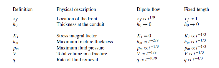
, as can be obtained conveniently based on a scaling analysis of the governing partial differential–integral system (2.1a
,
b
) and the condition of dipole moment conservation (3.1). Detailed discussions on this dipole-flow regime were provided in a recent work (Zheng Reference Zheng2024b
), the physics of which could be related to the dipole-flow regime of a viscous gravity current (e.g. King & Woods Reference King and Woods2003; Dudfield & Woods Reference Dudfield and Woods2012). Interestingly, the self-similarity of the dipole type is an incomplete one, for which we can only determine the scaling exponents at intermediate times, while the prefactors are under the influence of the initial condition (e.g. Barenblatt Reference Barenblatt1996).
3.2.
The fixed-length regime: when
$\Pi _k \gg 1$

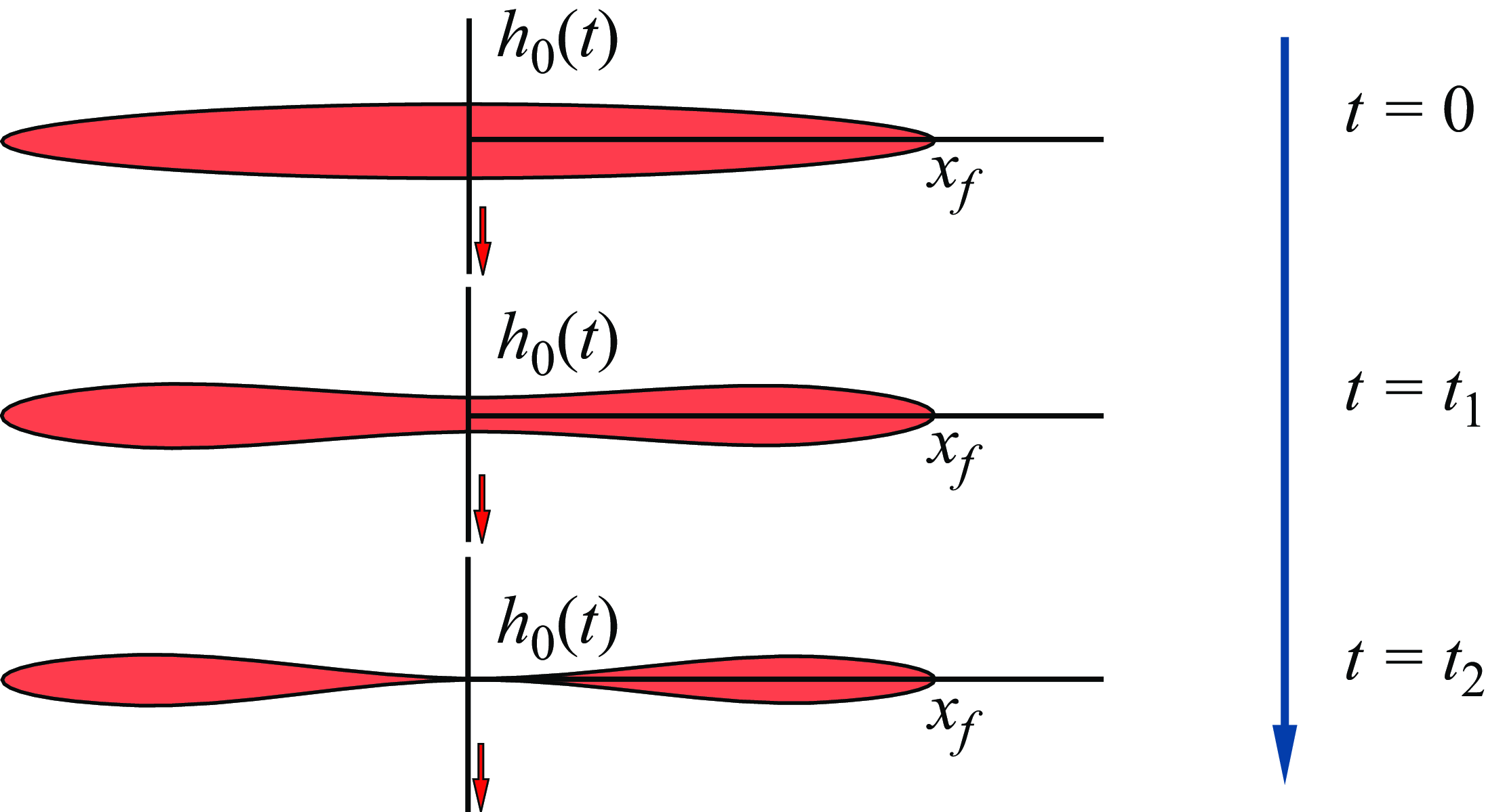
When the elastic solid is also brittle but does not heal at the fracture’s tip once broken, upon fluid removal through a conduit, the fracture evolves eventually into a pinned-front regime, as shown in figure 4.
3.2.1. Scaling analysis
The fixed-length regime of viscous backflows with extraction/suction when
 $\Pi _e \gt 0$
following hydraulic fracturing, when the brittle material does not recover its toughness after fracturing. The fracture’s thickness approaches zero at the centre
 $h_0(t) \to 0^+$
eventually, while the frontal location
 $x_f$
remains pinned in the toughness-dominated regime (
 $\Pi _k \gg 1$
) without material healing.

In the current context of fluid removal following creation of a plane fracture, we observed that, imposing the propagation condition (2.4) in the numerical scheme with
 $\Pi _k\gt 0$
, the front eventually becomes pinned after an initial spreading period. If
 $\Pi _k$
is sufficiently large, in particular, the extent of initial spreading in such a toughness-dominated regime becomes negligibly small as if the front remains pinned during the entire process of fluid removal, as shown in figure 4. That is, when
 $\Pi _e \gt 0$
(with extraction), the fracture thickness approaches zero at intermediate times at both the inlet (
 $x=0$
) of the conduit and the location of the pinned front (
 $x=x_f$
), while the fracture length remains pinned (i.e.
 $x_f$
is now time independent). This is illustrated by the time-dependent numerical solutions in figure 5, where we used
 $(\Pi _c,\Pi _e) = (1,40)$
and
 $\Pi _k = 2$
as a representative example. We note also that since there exists no fluid film for the region of
 $x \in (x_f(t),\infty )$
ahead of the fluid front, the value of
 $p(x,t)$
in this region is not really fluid pressure, but is the normal stress
 $\sigma _{yy}(x,y=0,t)$
induced at point
 $x$
within the solid due to a fracture aperture
 $h(x,t)$
in the region of
 $x \in [0, x_f(t))$
. This is true for all related figures in the present work.
It is of interest to note that we would expect a
 $h \propto t^{-1/3}$
scaling for this stage of fluid drainage and fracture deflation. Accordingly, the pressure
 $p$
and stress intensity factor
 $K$
also decrease according to the
 $t^{-1/3}$
power law. Hence, we expect that
 \begin{equation} x \propto 1, \qquad h \propto t^{-1/3},\qquad p \propto t^{-1/3}\quad \mbox {and}\quad K \propto t^{-1/3} \end{equation}
at intermediate times. It is also of interest to understand the time evolution of the total fluid volume within the fracture and rate of fluid removal, which now scale as
 \begin{equation} V = \int _{-x_f}^{x_f} h(x,t)\,\textrm { d}x \propto t^{-1/3}\quad \mbox {and}\quad q \propto t^{-4/3} \end{equation}
at intermediate times. These scaling behaviours are also consistent with our time-dependent numerical solutions with
 $\Pi _k = 2$
after an initial transition period, as shown in figure 6, where we have tracked the frontal location
 $\bar {x}_f$
, maximum thickness
 $\bar {h}_m$
, maximum pressure
 $\bar {p}_m$
, the stress intensity factor
 $\bar {K}$
and the total volume
 $\bar {V}$
of the fluid. The parameters were made dimensionless here using the same characteristic length, time and pressure scales as those in (2.5) for dipole fractures, when the material toughness is
 $\Pi _k = 0$
.
Numerical solutions for the time evolution of the profile shape
 $\bar {h}(\bar {x}, \bar {t})$
and pressure distribution
 $\bar {p}(\bar {x}, \bar {t})$
for
 $(\Pi _c,\Pi _e,\Pi _k)=(1,40,2)$
at
 $\bar {t} = 0.2 \times \{0-8\}$
. We used
 $N=200$
for a domain of length
 $L_d=1$
here. The inset of (b) shows the evolution of the pressure singularity at the fracture’s front, the accuracy of which depends significantly on the grid size.

In addition, we can rescale the raw numerical solutions of
 $\bar {h}(\bar {x}, \bar {t})$
and
 $\bar {p}(\bar {x}, \bar {t})$
in figure 6 based on the maximum values of
 $\bar {h}_m(\bar {t})$
and
 $\bar {p}_m(\bar {t})$
, and this leads to very good collapse onto universal curves, as shown in figure 7. Later, we show that indeed self-similar solutions exist for both the fracture’s profile shape and the pressure distribution within the liquid film. We also included the prediction of the self-similar solutions in the same figure 7, which illustrates very good agreement with the collapsed time-dependent numerical solutions. The physics of this regime of self-similar drainage with fixed length is then related to the dynamic drainage of a gravity current from a finite edge (e.g. Zheng et al. Reference Zheng, Soh, Huppert and Stone2013).
3.2.2. Self-similar solution with fixed length
We can also explore self-similar solutions for such a fixed-length regime by denoting
 $\zeta \equiv \bar {x} \in [0,\zeta _f]$
, where
 $\zeta _f = \bar {x}_f$
. The self-similar profile shape and pressure are then explored in the form of
 $\bar {h}(\bar {x}, \bar {t}) = \bar {t}^{-1/3} \mathcal {K}(\zeta )$
and
 $\bar {p}(\bar {x}, \bar {t}) = \bar {t}^{-1/3} \mathcal {G}(\zeta )$
. The partial differential–integral system (2.6a
) and (2.9) now becomes
 \begin{align} \frac {1}{3} \mathcal {K} + \frac {\textrm { d}}{\textrm { d} \zeta }\left (\mathcal {K}^3\frac {\textrm { d} \mathcal {G}}{\textrm { d} \zeta }\right ) = 0, \end{align}
 \begin{align} \mathcal {G}(\zeta ) = - \int _{0}^{1} \frac {2s}{s^2-\zeta ^2}\frac {\textrm { d} \mathcal {K}}{\textrm { d} s}\textrm { d} s, \end{align}
subject also to the zero thickness conditions
 \begin{equation} \mathcal {K}(0) = 0\quad \mbox {and}\quad \mathcal {K}(\zeta _f) = 0. \end{equation}
Numerical solutions for the time evolution of the frontal location
 $\bar {x}_f(\bar {t})$
, maximum thickness
 $\bar {h}_m(\bar {t})$
, maximum pressure
 $\bar {p}_m(\bar {t})$
and the total fluid volume
 $\bar {V}(\bar {t})$
for representative values of
 $(\Pi _c,\Pi _e,\Pi _k)$
when
 $\Pi _k\gt 0$
(with extraction). The slopes in the log-log plots approach the predicted values after an initial transition period for all cases considered here.

We employ the numerical scheme described in the appendices of Zheng (Reference Zheng2024a ,Reference Zheng b ), which also illustrates the stability of the self-similar solutions. The key idea is to transform (2.6a ) and (2.9) into another time-dependent system, i.e.
 \begin{align} -\frac {\partial K}{\partial \tau } + \frac {1}{3} K + \frac {\partial }{\partial \zeta }\left (K^3\frac {\partial G}{\partial \zeta }\right ) = 0, \end{align}
 \begin{align} G(\zeta ,\tau ) = - \int _{0}^{1} \frac {2s}{s^2-\zeta ^2}\frac {\partial K}{\partial s}\textrm { d} s, \end{align}
using a new transform
 $\tau = \mbox {ln}\, \bar {t}$
and
 $\zeta = \bar {x}$
. Similar transforms have been employed previously to study the development of finite-time singularities of thin fluid threads (e.g. Eggers & Fontelos Reference Eggers and Fontelos2009). The only difference between (3.4a
,
b
) and (3.6a
,
b
) is the addition of an unsteady term
 $- \partial K/\partial \tau$
in (3.6a
) for the transformed profile shape. Note also that now
 $K(\zeta ,\tau )$
and
 $G(\zeta ,\tau )$
both also depend on
 $\tau$
in (3.6a
,
b
), with this new transform retaining the time dependence, and we then solve (3.6a
,
b
) until there is no time evolution observed for the (normalised) numerical solutions
 $K_m^{-1}K(\zeta /\zeta _f,\tau )$
and
 $G_m^{-1}G(\zeta /\zeta _f,\tau )$
based on the maximum values
 $K_m(\tau )$
and
 $G_m(\tau )$
at any particular time
 $\tau$
. The resulting time-independent solutions
 $K_m^{-1}K(\zeta /\zeta _f,$
 $\tau \to \infty )$
and
 $G_m^{-1}G(\zeta /\zeta _f,\tau \to \infty )$
for sufficiently large
 $\tau$
then provide the (normalised) self-similar solutions
 $\mathcal {K}_m^{-1}\mathcal {K}(\zeta /\zeta _f)$
and
 $\mathcal {G}_m^{-1}\mathcal {G}(\zeta /\zeta _f)$
of the original ordinary-differential–integral system (3.4a
,
b
) subject to boundary conditions (3.5a,b
).
We must also consider the propagation condition (2.12) due to the influence of material toughness, which is now transformed into
 \begin{equation} \frac {K(\zeta ,\tau )}{(\zeta _f-\zeta )^{1/2}} \bigg |_{\zeta \to \zeta _f^-}= e^{1/3\tau }\, \Pi _k. \end{equation}
Meanwhile, the flux boundary condition (2.10) at the location of the conduit is transformed into
 \begin{equation} K^3\frac {\partial G}{\partial \zeta }\bigg |_{\zeta =0} = -e^{\tau } \,\Pi _c\, G(0,\tau ) - e^{4\tau /3}\, \Pi _e. \end{equation}
The normalised self-similar solutions are also included in figure 7, which show good agreement with the appropriately rescaled and collapsed time-dependent numerical solutions.
The rescaled numerical solutions for the time evolution of both the profile shape
 $\bar {h}(\bar {x}, \bar {t})/\bar {h}_m(\bar {t})$
and pressure distribution
 $\bar {p}(\bar {x}, \bar {t})/\bar {p}_m(\bar {t})$
as a function of dimensionless horizontal location
 $\eta = \bar {x}/\bar {x}_f(\bar {t})$
. The rescaled time-dependent numerical solutions in figure 5(a,b) collapse onto universal curves at intermediate times, which also agree reasonably well with the self-similar solutions. We used 220 grids to calculate the self-similar solutions.

Note that this self-similar solution does not explicitly include the influence of material toughness
 $K_c$
. Its subtle influence is that the location of the front
 $\bar {x}_f$
now remains constant after an initial transition period. We hence expect that this solution develops first in the region near the conduit (
 $\bar {x} = 0$
) where the influence of flow is most important. This solution then develops gradually towards the location of the front (
 $\bar {x} = \bar {x}_f$
). Equivalently, there always exists a tip region of elliptic shape as
 $\bar {x} \to \bar {x}_f^-$
, the length of which shrinks with time as the self-similar solution develops. This is verified through the appropriately rescaled and collapsed time-dependent numerical solutions of (2.1a
,
b
) subject to IBCs (2.2a
–c), now also with the propagation condition (2.12). Indeed, good agreement also appears with the self-similar solutions of
 $\mathcal {K}(\zeta )$
and
 $\mathcal {G}(\zeta )$
. As a comparison, we have also included the elliptic shape
 \begin{equation} \mathcal {K}(\zeta ) = 2\left [\frac {1}{4}-\left (\zeta -\frac {1}{2}\right )^2\right ]^{1/2} \end{equation}
in figure 7(a), which actually provides a very good estimate for the profile shape for almost the entire domain after an initial transition period.
The regime diagram of viscous backflows following hydraulic fracturing of an elastic solid with extraction when
 $\Pi _e \gt 0$
: (I) the dipole-flow regime when the front continues to grow (
 $\Pi _k \to 0$
), and (II) the fixed-length regime (
 $\Pi _k \to \infty$
). Representative transient behaviours are also included for intermediate
 $\Pi _k$
.

3.3. Backflow regimes following hydraulic fracturing
We have thus identified two different limiting regimes with extraction when
 $\Pi _e \gt 0$
, as shown in figure 8, depending on the value of the dimensionless material toughness
 $\Pi _k \equiv K_c[32(1-\sigma ^2)^3/3\pi \mu qE^3]^{1/4}$
. In both regimes, self-similar solutions can be obtained to describe the intermediate behaviours, with key scaling behaviours also summarised in table 2, including the scaling results for the location of the fracture’s front
 $x_f(t)$
, maximum fracture thickness
 $h_m(t)$
, maximum fluid pressure
 $p_m(t)$
, total fluid volume within the fracture
 $V(t)$
and rate of fluid removal
 $q(t)$
. We also observed that the value of
 $(\Pi _c,\Pi _e, \Pi _k)$
could impact the duration of the transient period for the thickness of the fracture to approach zero at the conduit (
 $x=0$
) and, hence, the time needed for the development of the self-similar behaviours.
Key features of fracture deflation at intermediate times during fluid removal through a narrow conduit at the centre when
 $\Pi _e\gt 0$
(with extraction). We summarise the scaling results in both the dipole-flow and fixed-length regimes.

For intermediate values of
 $\Pi _k$
, different transient behaviours are expected and also observed from numerical solutions of the partial differential–integral system (2.6a
,
b
) with appropriate IBCs and propagation condition. For example, once pressure is released at the outlet of the conduit, the length of a fracture is observed to grow for an initial period of time before it remains constant at intermediate times. These transient behaviours are included also in the regime diagram, which connects the two limiting regimes that exhibit dipole-flow and fixed-length behaviours, respectively. In any scenarios described here with extraction (
 $\Pi _e \gt 0$
), eventually, once the front becomes pinned, the profile shape and pressure evolution can both be described by the self-similar solution presented in this section.
3.4.
Purely elasticity-driven fracture deflation when
$\Pi _e=0$

As of now the discussion has focused primarily on the backflow situation with extraction/suction when
 $\Pi _e \gt 0$
. A primary feature is that the thickness of the fracture approaches zero at the centre
 $\bar {x} = 0$
at intermediate times, i.e.
 $\bar {h}(0,\bar {t}) \to 0$
, which allows analytical progress to be made with and without the influence of material toughness. We also recognise that it could be of interest to further discuss the situation of purely elasticity-driven backflow during fracture deflation without the influence of extraction, when
 $\Pi _e = 0$
. Such a situation is related to the laboratory experiments in transparent solid gelatins performed by Lai et al. (Reference Lai, Zheng, Dressaire, Ramon, Huppert and Stone2016a
), as we discuss briefly before we close this section. In particular, we report a different self-similar solution that is consistent with previous experimental observations.
Numerical solutions for the time evolution of the profile shape
 $\bar {h}(\bar {x}, \bar {t})$
and pressure distribution
 $\bar {p}(\bar {x}, \bar {t})$
when
 $(\Pi _c,\Pi _e,\Pi _k)=(1,0,2)$
at
 $\bar {t} = 0.2 \times \{0-8\}$
for purely elasticity-driven fracture deflation. We used
 $N=200$
for a domain of length
 $L_d=1$
here. The inset of (b) shows the evolution of the pressure singularity at the fracture’s front, the accuracy of which depends significantly on the grid size.

The rescaled numerical solutions for the profile shape
 $\bar {h}(\bar {x}, \bar {t})/\bar {h}_m(\bar {t})$
and pressure distribution
 $\bar {p}(\bar {x}, \bar {t})/\bar {p}_m(\bar {t})$
as a function of dimensionless horizontal location
 $\eta = \bar {x}/\bar {x}_f(\bar {t})$
for purely elasticity-driven fracture deflation. The rescaled time-dependent numerical solutions in figure 9(a,b) collapse onto universal curves at intermediate times, which also agree reasonably well with the self-similar solutions. We used 220 grids to calculate the self-similar solutions.

3.4.1. Self-similar solutions
Our time-dependent numerical solutions indicate that the thickness of the fracture remains positive at the location of the conduit (
 $\bar {x}=0$
), while the local pressure approaches zero at intermediate times, i.e.
 $\bar {p}(0,\bar {t}) \to 0$
, as shown in figure 9 when we impose
 $(\Pi _c,\Pi _e,\Pi _k)=(1,0,2)$
. This is an important feature of purely elasticity-driven fracture deflation and is fundamentally different from the situations with extraction. Correspondingly, when
 $\Pi _e = 0$
, the asymptotic behaviour at intermediate times would be different from the self-similar behaviours from solving (3.4a,
b
) subject to (3.5a,b
) when
 $\Pi _e \gt 0$
, as discussed in the previous section, because the zero thickness boundary condition (3.5a
), which corresponds to
 $\bar {h}(0,\bar {t}) \to 0$
, no longer applies.
Nevertheless, our numerical solutions also indicate that the time-dependent profile shapes and pressure distributions can still be rescaled appropriately (normalised) to collapse onto universal shapes at intermediate times, which suggests the existence of self-similarity for purely elasticity-driven fracture deflation. An example calculation is shown in figure 10, when we rescale the time-dependent numerical solutions of figure 9 based on the maximum thickness
 $\bar {h}_m(\bar {t})$
and pressure
 $\bar {p}_m(\bar {t})$
. The time-dependent numerical solutions also suggest the same scaling behaviours (3.2) and (3.3) for the time evolution of the frontal location
 $\bar {x}_f(\bar {t})$
, maximum thickness
 $\bar {h}_m(\bar {t})$
, maximum pressure
 $\bar {p}_m(\bar {t})$
and total fluid volume
 $\bar {V}(\bar {t})$
, as shown in figure 11 and summarised in table 3.
Numerical solutions for the time evolution of the frontal location
 $\bar {x}_f(\bar {t})$
, maximum thickness
 $\bar {h}_m(\bar {t})$
, maximum pressure
 $\bar {p}_m(\bar {t})$
and the total fluid volume
 $\bar {V}(\bar {t})$
for representative values of
 $(\Pi _c,\Pi _k)$
when
 $\Pi _e=0$
for purely elasticity-driven fracture deflation. The slopes in the log-log plots approach the predicted values after an initial transition period for all cases considered here.

Key features of purely elasticity-driven fracture deflation at intermediate times during fluid removal through a narrow conduit without suction (
 $\Pi _e = 0$
). The scaling behaviours summarised here apply when the influence of material toughness is included (
 $\Pi _k \gt 0$
).

We hence expect that the definition of the self-similar solutions
 $\bar {h}(\bar {x}, \bar {t}) = \bar {t}^{-1/3} \mathcal {K}(\zeta )$
and
 $\bar {p}(\bar {x}, \bar {t}) = \bar {t}^{-1/3} \mathcal {G}(\zeta )$
continues to apply here, where
 $\zeta \equiv \bar {x} \in [0,\zeta _f]$
. Moreover, the corresponding self-similar solutions
 $\mathcal {G}(\zeta )$
and
 $\mathcal {K}(\zeta )$
can also be obtained from solving the same ordinary-differential–integral system (3.4a
,
b
), but now subject to a different set of boundary conditions
 \begin{equation} \mathcal {G}(0) = 0\quad\mbox {and}\quad \mathcal {K}(\zeta _f) = 0, \end{equation}
which indicate zero pressure at the centre and zero thickness at the front. Interestingly, the (normalised) self-similar solutions
 $\mathcal {K}_m^{-1}\mathcal {K}(\zeta /\zeta _f)$
and
 $\mathcal {G}_m^{-1}\mathcal {G}(\zeta /\zeta _f)$
can still be obtained from solving the time-dependent system of (3.6a
,
b
) with appropriately transformed flux conditions at both ends of the domain and the propagation condition (3.7). Again, the idea is to solve the time-dependent system until there is no time evolution, and indeed the new boundary conditions (3.10a,b
) are satisfied eventually.
To further illustrate these interesting behaviours, we then rescale appropriately the time-dependent numerical solutions in figure 9 when
 $(\Pi _c,\Pi _e,\Pi _k)=(1,0,2)$
, and we have indeed observed very good collapse of the rescaled numerical solutions at intermediate times, as shown in figure 10. The self-similar solutions from solving (3.6a
,
b
) are also included in the same figure, which shows reasonable agreement with the normalised and collapsed time-dependent numerical solutions for both the profile shape and pressure distribution. As a comparison, we also included the elliptic solution (3.9) in figure 10(a), which approximates reasonably well the self-similar profile shape in a region close to the front (
 $\zeta = \zeta _f$
). Near the conduit (
 $\zeta = 0$
) however, the elliptic solution (3.9) fails to describe the profile shape, as the inlet thickness remains positive. We also note that the inlet thickness
 $\mathcal {K}_m^{-1}\mathcal {K}(0) \approx 0.89$
(with 220 space grids imposed) of the normalised similarity solution appears to be independent of the value of
 $(\Pi _c,\Pi _k)$
, based on further numerical tests. This seems reasonable, because both the time-independent governing equations (3.4a
,
b
) and the boundary conditions (3.10a,b
) for the similarity solutions are independent of
 $(\Pi _c,\Pi _k)$
.
3.4.2. Experimental observations
We provide brief comments here on available experimental observations from literature on viscous backflows from elastic solids during fracture deflation (e.g. Lai et al. Reference Lai, Zheng, Dressaire, Ramon, Huppert and Stone2016a ). These experiments were typically performed in elastic solids such as transparent solid gelatins of relatively large size, such that radial fractures of the penny shape are typically generated. The theory here is made in the Cartesian configuration but is able to explain the key trends of the experimental observations qualitatively.
Upon pressure release, the fracturing fluid flows out of a penny-shaped fracture through a narrow conduit located approximately at the centre of the fracture. A meniscus is generated between the fracturing fluid and air within the long conduit, which is different from the current model. But this is not expected to significantly influence the qualitative trend of the fracture shape evolution as well. It is typically observed that a fracture takes approximately an elliptic shape initially for backflow with its front located at approximately a fixed location within the time scale of the experiments. As time progresses in these experiments, the central region near the location of the conduit starts to become flat and the profile shape departs slightly from being perfectly elliptic. These experiments proceeded typically until there was less than 10 % of the fracturing fluid by volume within the elastic solid.
Our theoretical model generates very similar results for fracture shape evolution by imposing a relatively large dimensionless material toughness
 $\Pi _k$
and relatively small
 $\Pi _c$
that describes the relative strength of elasticity-driven backflow. Typical numerical results of (2.6a
,
b
) were provided in figure 12(b) for the profile shape evolution, imposing
 $\{\Pi _c,\Pi _e,\Pi _k\} = \{1,0,2\}$
for the subsequent process of backflow without suction. The numerical results compare well the experimental observations in figure 12(a), qualitatively. The universal profile shape shown in figure 10(a) after appropriate rescaling also appears to be consistent with the experimental observations at intermediate times. Meanwhile, we can also track the total volume of the fluid within the elastic solid, as shown in figure 12(b) as well, which provides good agreement with experimental observations in figure 12(a) as well. The
 $\bar {V} \propto \bar {t}^{-1/3}$
scaling law is also observed at late times, when viscous thin film flow is dominant within the fracture. We consider that these theoretical and experimental observations are in accord. However, it is not appropriate to apply the scaling laws to the transient stage, when the influence of viscous flow within the conduit is still important.
Comparison between (a) experimental observations of the evolution of the profile shapes and rescaled fluid volume within a fracture in Lai et al. (Reference Lai, Zheng, Dressaire, Ramon, Huppert and Stone2016a
) and (b) numerical solutions of (2.6a
,
b
) with appropriate IBCs and propagation condition without healing, imposing
 $\{\Pi _c,\Pi _e,\Pi _k\} = \{1,0,2\}$
, where we tracked the time evolution of the profile shapes
 $\bar {h}(\bar {x}, \bar {t})$
and the total fluid volume
 $\bar {V}(\bar {t})$
within the elastic solid as well. We used 200 grid points on a domain of
 $\bar {x} \in [0,1]$
in (b) for a sense of the numerical error. In (a),
 $w(r,t)$
represents the half-thickness of a fracture.

For a more quantitative comparison between theoretical and experimental results of penny-shaped fracture deflation, one could consider analogous models in the radial configuration. One major difference, compared with the Cartesian configuration of the present work, lies in the kernel of the integral equation for elastic pressure. In the radial geometry, complete elliptic integrals of the first and second kinds present in the pressure equation, as shown in Spence & Sharp (Reference Spence and Sharp1985). The Reynolds equation and global mass conservation equation also need to be slightly modified accordingly to address the influence of radial geometry, but this is well understood for any type of gravity current and thin film problems. For the injection/fracturing process, it has been shown that scaling analysis can still be applied to obtain quick insights on the growth laws for the length and thickness evolution of penny-shaped hydraulic fractures and parametric dependence (e.g. Spence & Sharp Reference Spence and Sharp1985; Lai et al. Reference Lai, Zheng, Dressaire, Wexler and Stone2015; OKeeffe et al. Reference OKeeffe, Huppert and Linden2018). However, detailed asymptotic solutions for the profile shape and pressure distribution could vary significantly between plain strain fractures and penny-shaped radial fractures (e.g. Spence & Sharp Reference Spence and Sharp1985; Savitski & Detournay Reference Savitski and Detournay2002; Detournay Reference Detournay2004). Detailed theoretical analysis on the deflation of penny-shaped hydraulic fractures from fluid withdrawal through narrow conduits could still be of interest for future work.
4. Summary and final remarks
4.1. Brief summary
We have provided a theoretical model to describe the dynamics of viscous backflows following hydraulic fracturing of an elastic solid upon fluid withdrawal through a narrow conduit located at the centre (
 $x=0$
). The current work deals primarily with the influence of material toughness at the fracture tip, compared with a previous work focusing primarily on the coupled balance of viscous flow and elastic deformation (Zheng Reference Zheng2024b
). This is characterised first by an additional dimensionless control parameter, i.e. the dimensionless toughness
 $\Pi _k$
. In the toughness-dominated regime
 $(\Pi _k \gg 1)$
, the model leads to an additional limiting regime of fluid removal at intermediate times, i.e. the fixed-length regime. This regime is summarised also in a regime diagram in figure 8, together with the dipole-flow regime when
 $\Pi _k = 0$
, as identified in Zheng (Reference Zheng2024b
).
Of particular interest is that we can find self-similar solutions to describe the intermediate dynamics in both the dipole-flow and fixed-length regimes when
 $\Pi _e \gt 0$
with external extraction (suction). The similarity solutions are verified based on the rescaled numerical solutions of the original partial differential–integral system (2.6a
,
b
), imposing appropriate IBCs and propagation condition. Key features in these limiting regimes of self-similar backflows during fracture deflation are also summarised in table 2 with a focus on the time evolution of scales of important physical properties. The observed transient behaviours for intermediate
 $\Pi _k$
are also briefly discussed, which are consistent with the regime diagram of figure 8.
We also explored the special situation of purely elasticity-driven fracture deflation without suction when
 $\Pi _e = 0$
. In this case, it is found that at intermediate times the local pressure approaches zero, i.e.
 $\bar {p}(0,\bar {t}) \to 0$
, at the location of the conduit. This is completely different from the situation with extraction when the fracture thickness approaches zero at intermediate times, i.e.
 $\bar {h}(0,\bar {t}) \to 0$
. Different self-similar solutions are obtained, as summarised also in figure 13, to describe the profile shape and pressure evolution for purely elasticity-driven fracture deflation but with the same scaling behaviours. These predictions appear to be consistent with previous experimental observations of viscous backflows from hydraulic fractures in solid gelatins.
Self-similar solutions from hydraulic fracturing towards fracture deflation in the material toughness-dominated regime (
 $\Pi _k \gg 1$
): (a) with the influence of external extraction (
 $\Pi _e \gt 0$
) as discussed in § 3.2, and (b) without suction (
 $\Pi _e = 0$
) as discussed in § 3.4.

4.2. The influence of finite thickness/pressure values at the conduit
In our numerical results, we have observed that with extraction (
 $\Pi _k\gt 0$
), the thickness approaches zero at the location of the conduit (
 $\bar {x} = 0$
), while pressure
 $\bar {p}_0 (\bar {t}) \equiv \bar {p}(0,\bar {t})$
approaches a constant that is related to the value of
 $\Pi _e$
. In contrast, without suction (
 $\Pi _k=0$
), the pressure approaches zero at the conduit, while the thickness
 $\bar {h}_0(\bar {t}) \equiv \bar {h}(0,\bar {t})$
decreases but remains finite. Nevertheless, it is also observed that the prediction of the scaling analysis and self-similar solutions work reasonably well in both cases at intermediate times, even with the existence of these finite values at
 $\bar {x} = 0$
. This is not surprising because of the following two different limiting regimes of fracture deflation at intermediate times: (i) When
 $\Pi _k\gt 0$
, the maximum pressure scales as
 $\bar {p}_m \propto \bar {t}^{-1/3}$
, and hence, the ratio
 $\bar {p}_0/\bar {p}_m \to \infty$
when
 $\bar {t} \gg 1$
. We could also obtain an estimate for the length of the transient time as
 $\bar {t} \gg \Pi _e^{-3}$
for
 $\bar {p}_0/\bar {p}_m \to \infty$
to apply, and it is seen that a greater extraction parameter
 $\Pi _e$
corresponds to a shorter transient time period, which is consistent with the time-dependent numerical results. (ii) When
 $\Pi _k=0$
, the maximum thickness scales as
 $\bar {h}_m \propto \bar {t}^{-1/3}$
, and it appears that
 $\bar {h}_0 \propto \bar {t}^{-1/3}$
as well, such that
 $\bar {h}_0/\bar {h}_m$
approaches a constant. Hence, the finite thickness/pressure values at the location of the conduit do not actually introduce additional scales at intermediate times (
 $\bar {t} \gg 1$
), and eventually their influence on the existence of self-similarity becomes negligible.
4.3. Fracture deflation due to fluid leakage into permeable solids
The pinned-front behaviour in the toughness-dominated regime is also consistent with previous understanding known as the Stevenson condition for fracture deflation (e.g. Roper & Lister Reference Roper and Lister2007). Nevertheless, fluid leakage into elastic solids could possibly lead to distinct deflation dynamics such as the frontal receding behaviours. This is an important situation of practical interest and has been the focus of a series of previous studies (e.g. Peirce & Detournay Reference Peirce and Detournay2022a ,Reference Peirce and Detournay b ,Reference Peirce and Detournay c ; Peirce Reference Peirce2022), dealing with different interesting variations of the coupled thin film flow, elastic deformation, material breaking and fluid leakage. From the modelling point of view, instead of imposing an appropriate flux boundary condition at the origin to account for fluid removal through a conduit, appropriate sink terms are needed to be incorporated into the Reynolds equation for the profile shape evolution to account for the influence of fluid leakage into permeable elastic solids. Notably, analogous problems exist in the gravity current literature (see, e.g. Pritchard et al. Reference Pritchard, Woods and Hogg2001; Yu et al. Reference Yu, Zheng and Stone2017; Liu et al. Reference Liu, Zheng and Stone2017), where fluid volume of a gravity current decreases due to leakage and frontal receding dynamics is also observed at intermediate times.
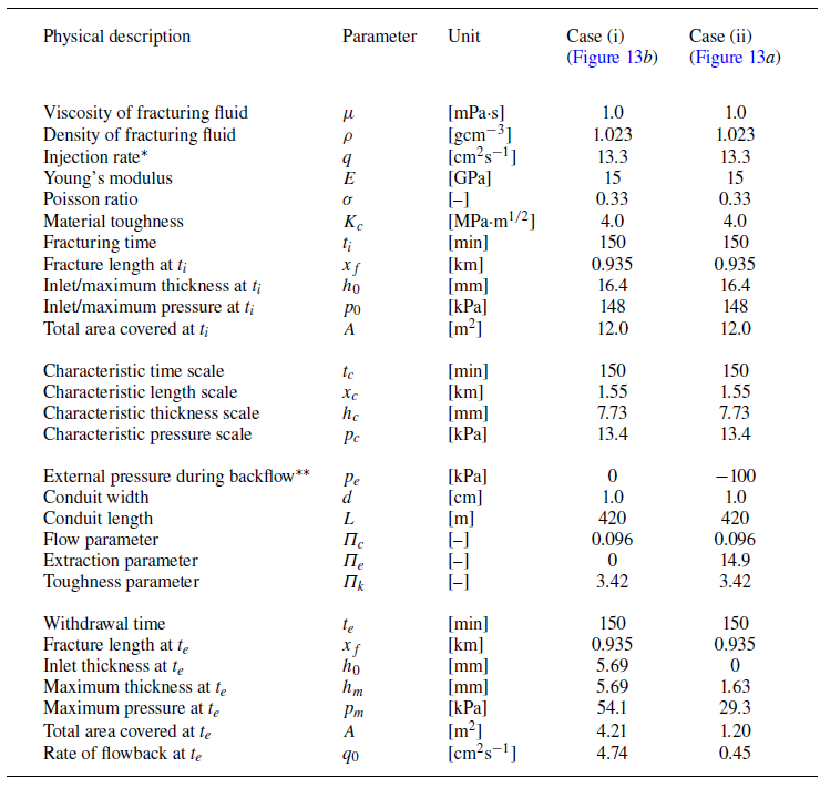
Example calculations of fluid withdrawal from an initial fracture in a rock formation: (i) without external extraction as discussed in § 3.2, and (ii) with extraction as discussed in § 3.4. *The injection rate
 $q$
into the positive half-domain is estimated by a volumetric rate of 0.0265 m
 $^3$
s−1 divided by a length of 200 m perpendicular to the plane of paper. **The external pressure
 $p_e$
is estimated based on the atmospheric pressure. We used
 $N=150$
for a domain of length
 $L_d=1$
here for a sense of the numerical error.

4.4. Potential implications
The model and solutions might find applications in environmental and industrial processes such as hydraulic fracturing of rock formations for the recovery of fluid-phase resources such as crude oil, shale gas and geothermal energy (e.g. Bickle et al. Reference Bickle, Goodman, Mair, Roberts, Selley, Shipton, Thomas and Younger2012) and underground energy storage in hydraulic fractures (e.g. Bunger et al. Reference Bunger, Lau, Wright and Schmidt2023). For example, the fracture length evolution predicted is related to the outreach into a rock formation upon pressure release, which is an important factor in the amount of resources that could potentially be recovered. The fracture thickness evolution is related to the permeability of pathways for fracturing fluid to flow out and faster transport of gas and thermal energy to occur. Such information could be of use to evaluate the performance of resource recovery technologies and potential environmental risks. We do not continue detailed discussions here and conclude this paper by pointing out that (i) geophysical and operational data need to be substituted into the dimensionless model to obtain solutions with units, and (ii) one needs to choose the correct solutions in appropriate regimes based on the specific values of the dimensionless parameters.
Before we end this paper, we provide an example calculation of fluid withdrawal from an initially created hydraulic fracture in a rock formation that is 420 m underneath the ground surface, with detailed geophysical and operational parameters summarised in table 4, estimated based on previous reports (e.g. Lister Reference Lister1990b
; Savitski & Detournay Reference Savitski and Detournay2002; Bunger et al. Reference Bunger, Lau, Wright and Schmidt2023). The Young’s modulus is
 $E = 15\,\rm GPa$
, the Poisson ratio is
 $\sigma = 0.33$
and material toughness is
 $K_c = 4.0$
MPa
 $\cdot$
m
 $^{1/2}$
for the rock, which is initially fractured by a fracturing fluid of viscosity
 $\mu = 1.0\,\rm mPa.s$
and density
 $\rho = 1.023\,\rm g\,cm^-{^3}$
. We consider two cases for fracture deflation with fluid removal through a conduit of length
 $L = 420\,\rm m$
and width
 $d=1\,\rm cm$
, with the only difference being the external pressure imposed at the outlet of the narrow conduit: In case (i) we consider
 $p_e = 0\,\rm MPa$
without suction, while in case (ii) we consider
 $p_e = -0.1\,\rm MPa$
for the influence of external extraction based on the atmospheric pressure. The initial fracturing time is fixed at
 $t_i = 150$
min, while the extraction time is also set as
 $t_e = 150$
min in both cases. Other geophysical and operational parameters are also maintained as the same for both cases, and within the conduit we have
 $Re_d \approx 1330$
, so the flow is laminar and (2.3) applies for the flow rate.
In the corresponding situations, we obtain
 $\Pi _c \approx 0.096$
and
 $\Pi _k \approx 3.42$
for cases (i) and (ii), while we obtain
 $\Pi _e = 0$
for case (i) and
 $\Pi _e \approx 14.9$
for case (ii). The characteristic time scale is chosen as
 $t_c = 150\,\rm min$
, while the characteristic length, thickness and pressure scales are obtained as
 $x_c \approx 1.55\,\rm km$
,
 $h_c \approx 7.73\,\rm mm$
and
 $p_c \approx 13.4\,\rm kPa$
. All of these values seem reasonable, compared with field data. We then numerically solve the problem of coupled thin film flow and elastic deformation to provide the time evolution of the profile shape and pressure distribution based on the present model, with key features of the numerical results summarised in table 4 as well, now with units. As we can see that with extraction the fracture’s thickness at the conduit could become significantly smaller than its maximum value during fluid withdrawal, which leads eventually to fracture closing. It is sometimes observed in the field that a fracture can close at the well bore during backflow, which is then consistent with the present theory and its occurrence could be significantly under the influence of external extraction.
Acknowledgements
We would like to thank the anonymous reviewers for very helpful comments on this work.
Funding
Partial support is acknowledged from a QJMAM award (No. 1017777) and NSFC (No. 12272235). This work was also partially supported by the Program for Professor of Special Appointment (Eastern Scholar, No. TP2020009) at Shanghai Institutions of Higher Learning.
Declaration of interests
The authors report no conflict of interest.
Appendix A. Numerical scheme
We briefly present a finite volume scheme that is employed to solve the nonlinear non-local system (2.6a
,
b
) subject to appropriate IBCs and propagation conditions for the coupled evolution of the fracture’s profile shape and pressure distribution within the fluid film. Very similar schemes have been employed in previous studies of hydraulic fracturing in Hele–Shaw cells (Zheng Reference Zheng2024
a) and gravity current propagation in porous layers (e.g. Zheng et al. Reference Zheng, Guo, Christov, Celia and Stone2015; Hinton & Woods Reference Hinton and Woods2018). In this section we remove the bars for the dimensionless variables
 $x$
,
 $t$
,
 $h$
and
 $p$
for simplicity.
We solve the problem within the domain of
 $x \in [0,L_d]$
, and the grid size is chosen as
 $\triangle x = L_d/N$
, where
 $N$
is the grid number. The time step is chosen as
 $\triangle t = c \triangle x^3$
, with the constant
 $c$
typically being of order
 $10^{-2}$
to obtain stable solutions in our code (which is explicit in time). Numerical solutions for
 $h(x,t)$
and
 $p(x,t)$
, denoted by
 $h_n^i$
and
 $p_n^i$
, respectively, are then provided at discretised locations of each space grid
 $x_n = (n-1/2)\triangle x$
for
 $n=1,2,\ldots N$
and time step
 $t_i = i \triangle t$
for
 $i = 0,1,2,\ldots ,I$
. The simulation then ends at any target time
 $t_f = I\triangle t$
of interest. Then, the discretised form of the Reynolds equation (2.6a
) is given by
 \begin{equation} h_n^{i+1} = h_n^i - \frac {\triangle t}{\triangle x} \left (q_{n+1/2}^i - q_{n-1/2}^i\right ) \end{equation}
for
 $i=0,1,2,\ldots ,I$
and
 $n=2,3,4,\ldots ,N-1$
, where the fluxes are defined at the boundary between two neighbouring cell-centred grids as
 \begin{equation} q_{n+1/2}^i = -\left (\frac {h_{n+1}^i+h_{n}^i}{2}\right )^3\frac {p_{n+1}^i-p_n^i}{\triangle x}\quad\mbox {and}\quad q_{n-1/2}^i = -\left (\frac {h_{n}^i+h_{n-1}^i}{2}\right )^3\frac {p_{n}^i-p_{n-1}^i}{\triangle x}. \end{equation}
At the two ends of the domain
 $n=1$
and
 $n=N$
, the fluxes are provided by
 $q_{1/2}^i=1$
and
 $q_{N+1/2}^i=0$
for the initial fracturing process. For the subsequent process of fracture deflation (backflow), the flux
 $q_{1/2}^i$
is modified to
 $q_{1/2}^i = -\Pi _c p_1^i - \Pi _e$
to account for the influence of fluid withdrawal through the conduit. For physical reasons, it is also required that
 $h_n^i \geqslant 0$
for any
 $n$
and
 $i$
throughout the evolution. The discretised pressure
 $p_n^i$
, meanwhile, is provided by the integral equation (2.6b
) as
 \begin{equation} p_n^i = - \left [\sum _{k=1}^{n_f} \frac {h_{k+1}^i-h_k^i}{(x_{k+1}+x_k)/2-x_n} + \sum _{k=1}^{n_f} \frac {h_{k+1}^i-h_k^i}{(x_{k+1}+x_k)/2+x_n}\right ], \end{equation}
where
 $n_f \in [1,N]$
denotes the location of the front where the fracture thickness is zero. Note that the form of (A3) has accounted for the contribution of elastic deformation on pressure from both the negative and positive sides of the domain. Providing any initial condition such as
 $h_n^{0} = 0$
, the aforementioned scheme is ready to provide numerical solutions for the coupled evolution of profile shape
 $h_n^i$
and pressure distribution
 $p_n^i$
. The scheme is explicit in time and second order in space.
When the influence of material toughness is non-negligible, we must also include a propagation condition (2.12), which is given by
 \begin{equation} \frac {h_{n_f-1}^i}{(x_{n_f}-x_{n_f-1})^{1/2}} = \Pi _k. \end{equation}
This is included as an additional justification on whether the fracture propagates or not at any time step
 $i$
. At each time step, if the dimensionless stress intensity factor (left-hand side of (A4)) is smaller than
 $\Pi _k$
, no propagation is allowed so
 $n_f$
remains as its previous value. In contrast, if it is greater than
 $\Pi _k$
, propagation is allowed, and the evolution of
 $h(x,t)$
and
 $p(x,t)$
and the frontal location
 $n_f$
are then determined by the finite volume scheme with appropriate flux conditions imposed at the two ends of the domain. This is the only difference between the present work and the previous work on the dipole self-similarity of fracture deflation (effectively by setting
 $\Pi _k=0$
) without the influence of material toughness (Zheng Reference Zheng2024b
). Typically, a grid number N between 150–300 is chosen such that a reasonably good convergence is observed for the numerical solutions of
 $h_n^i$
and
 $p_n^i$
in the bulk region and the frontal location
 $x_f(t)$
. The grid number
 $N$
in the present work seems to be slightly greater than typical values in previous studies of hydraulic fracturing (e.g. Spence & Sharp Reference Spence and Sharp1985; Spence et al. Reference Spence, Sharp and Turcotte1987; Lister Reference Lister1990a,Reference Listerb
; Roper & Lister Reference Roper and Lister2007), and we are able to obtain stable solutions within a reasonable amount of time with Matlab on a personal computer. We must note the pressure singularity near the front
 $n_f$
is still under the influence of further grid refinement. However, numerical solutions of
 $h_n^i$
and
 $p_n^i$
in the bulk region and the frontal location are not significantly under the influence of grid refinement any more, which is of primary interest in the present work.
Example results of the initial fracturing process at three representative times
 $\bar {t} = \{0.8,0.9,1.0\}$
: (a) when
 $\Pi _k = 0$
in the viscous regime, and (b) when
 $\Pi _k = 2$
with significant influence of material toughness. The profiles shown here cover approximately 200–400 space grids for a sense of numerical error, in particular for the pressure singularity near the propagating front. The normalised profile shapes and pressure distributions are plotted against well-known self-similar solutions, shown as the symbols, in both the viscous regime in (a) and toughness regime in (b). The self-similar solutions are obtained from previous studies (e.g. Spence & sharp Reference Spence and Sharp1985; Detournay Reference Detournay2004). Note also that figure 14(a) was also included in the appendix of Zheng (Reference Zheng2024b
) to show how the numerical scheme works in the viscous regime.

To illustrate the influence of material toughness on the initial fracturing process, we include example results in figure 14 at three representative times
 $\bar {t} = \{0.8,0.9,1.0\}$
. The only difference between figures 14(a) and 14(b) is that in figure 14(a) we imposed
 $\Pi _k = 0$
such that hydraulic fracturing occurs in the viscous regime and fracture propagation is resisted only by the viscous drag of the thin film flow, while in figure 14(b) we impose
 $\Pi _k = 2$
such that fracturing is under significant influence of material toughness and fracture propagation is resisted predominantly by breaking the elastic material at the tip. It is clearly shown in figure 14(a,b) that as hydraulic fracturing approaches the toughness regime (
 $\Pi _k \to \infty$
), the profile shape approaches the elliptic shape as predicted successfully by quasi-steady theory and linear elastic fracture mechanics of a type I crack sustained by normal stresses, and the pressure remains approximately a constant within the domain of the fracture. One can also compare the rescaled solutions to verify the self-similar behaviours in either the viscous or the toughness regime and check also the corresponding frontal propagation laws. For example, we have included the well-known self-similar solutions for the profile shape and pressure distribution (e.g. from table 3 of Spence & Sharp (Reference Spence and Sharp1985) for the profile shape and figure 5 of Detournay (Reference Detournay2004) for the pressure distribution in the viscous regime) as symbols in both the viscous and toughness regimes in panels (a) and (b), and the favourable comparison provides further evidence that the finite volume scheme is good enough to obtain insights into different asymptotic regimes of hydraulic fracturing. No additional treatments are needed to capture the intermediate behaviours at transient times and for modest values of
 $\Pi _k$
. The point here is to show briefly, following the suggestion of a reviewer, that the numerical scheme is indeed able to distinguish the viscous (
 $\Pi _k = 0$
) and toughness (
 $\Pi _k \to \infty$
) regimes of hydraulic fracturing. The process of hydraulic fracturing within infinite elastic solids without the influence of buoyancy is considered better understood as of now, following a series of theoretical (e.g. Spence & Sharp Reference Spence and Sharp1985; Savitski & Detournay Reference Savitski and Detournay2002; Detournay Reference Detournay2004) and experimental efforts (e.g. Lai et al. Reference Lai, Zheng, Dressaire, Wexler and Stone2015, Reference Lai, Zheng, Dressaire and Stone2016b
; OKeeffe et al. Reference OKeeffe, Huppert and Linden2018).