1 Introduction
Laminar–turbulent transition of hypersonic boundary layers is of great technological importance for the development of high-speed vehicles (Reshotko Reference Reshotko2008) and as such, it has been and still remains a subject of extensive investigation (Fedorov Reference Fedorov2011; Zhong & Wang Reference Zhong and Wang2012). Similar to its subsonic counterpart, super- and hypersonic boundary-layer transition involves, in the case of relatively weak free-stream turbulence, four stages in sequence: receptivity, linear instability, nonlinear development and final breakdown into small-scale turbulence. Excepting perhaps the linear instability, these instabilities remain inadequately understood despite substantial research efforts in the last few decades.
The first stage, receptivity, refers to the process in which external disturbances in the ambient environment trigger internal oscillations, i.e. eigenmodes, in the boundary layer (Morkovin Reference Morkovin1969; Reshotko Reference Reshotko1976). Instability modes which may arise depend on the Mach number
 $M$
. In the subsonic regime, they are Tollmien–Schlichting (T–S) waves, which have a viscous origin. In the super- and hypersonic regimes, there exist multiple families of modes (Mack Reference Mack1984) including the so-called first Mack modes, which are continuation of T–S modes into the compressible regime, and the second Mack modes, which are essentially inviscid. On the other hand, external disturbances are present on the wall (such as surface roughness or waviness) and in the incoming flow. Within a linear approximation, a general unsteady disturbance in a uniform compressible flow can be decomposed into three independent elementary constituents: acoustic, vorticity and entropy modes (Kovasznay Reference Kovasznay1953). An acoustic mode corresponds to a pressure wave propagating through the moving fluid at the speed of sound, while vorticity and entropy modes represent respectively weak vorticity and temperature perturbations being convected passively by the mean flow. Usually, none of these disturbances alone can excite eigenmodes because their length and/or time scales differ from those of the latter. The main task of receptivity study is thus to identify scale-conversion mechanisms which produce an effective forcing with both the time and length scales matching those of the instability.
Breakthroughs towards understanding and predicting boundary-layer receptivity were made in the 1980s, when some crucial scale-conversion mechanisms were identified and described mathematically. Goldstein (Reference Goldstein1983) showed that a long-wavelength acoustic wave can interact with the non-parallel mean flow near the leading edge, first to excite the so-called Lam–Rott asymptotic eigensolution, which then undergoes wavelength shortening and finally evolves into an unstable T–S wave. Since the Lam–Rott mode experiences severe decay before reaching the neutral stability point, this mechanism is fairly weak. An efficient mechanism was proposed independently by Ruban (Reference Ruban1984) and Goldstein (Reference Goldstein1985). It involves the interaction between a sound wave and the mean-flow distortion caused by abrupt changes in the wall geometry (such as a hump or a junction of an elliptic leading edge with the straight portion of the plate). The unsteady forcing resulting from the interaction excites a T–S wave provided that the frequency of the sound and the length scale of the abrupt change are comparable with those of the T–S instability. The coupling coefficient was calculated using the triple-deck asymptotic formalism.
Duck, Ruban & Zhikharev (Reference Duck, Ruban and Zhikharev1996) considered the receptivity due to free-stream vortical disturbances interacting with a local roughness on a flat plate. They pointed out that although a vortical disturbance does not penetrate into the boundary layer, it can interact with the roughness-induced steady perturbation at the outer edge of the boundary layer. Wu (Reference Wu2001a ) presented a second-order asymptotic theory and demonstrated that irrespective of the vertical structure of the vortical disturbance, the receptivity can be fully characterized by its slip velocity at the edge of the boundary layer. This allowed for quantitative comparisons with the experimental data of Dietz (Reference Dietz1999), and an excellent agreement was found. Wu (Reference Wu2001b ) investigated the distributed receptivity due to acoustic or vortical disturbances interacting with a wavy wall. The forcing resonates with a neutral T–S mode in a fairly extended vicinity of the lower-branch neutral curve, and as a result the receptivity is much stronger than in the case of an isolated roughness.
A rather different mechanism of generating T–S waves was proposed by Wu (Reference Wu1999). It involves the interaction between a vortical disturbance and a sound wave with suitable frequency and wavenumbers to generate a forcing in resonance with a neutral mode. Since this mechanism does not resort to any form of surface inhomogeneity, it operates effectively in canonical boundary layers over smooth flat walls.
For supersonic boundary layers, possible instability modes have been identified and their characteristics, obtained by solving compressible Orr–Sommerfeld and Rayleigh equations, have been well documented (Mack Reference Mack1984). Relevant asymptotic descriptions have been presented by Smith (Reference Smith1989), Smith & Brown (Reference Smith and Brown1990) and Blackby, Cowley & Hall (Reference Blackby, Cowley and Hall1993) among others. Most calculations and theories neglected shocks, which are present when the aerodynamic body has a finite thickness. In the hypersonic regime, a shock arises even in a flat-plate boundary layer because of the strong viscous–inviscid interaction near the leading edge. The presence of a shock could influence instability as perturbations may be reflected between the shock and boundary, and this effect can, as was first recognized by Petrov (Reference Petrov and Kozlov1984), be accounted for by imposing the linearized Rankine–Hugoniot relations as boundary conditions on the linearized stability equations. Adopting these conditions and the high Reynolds number asymptotic framework of the triple-deck formalism, Cowley & Hall (Reference Cowley and Hall1990) analysed the stability of the boundary layer over a sharp wedge. They found that the presence of a shock gives rise to an infinite but countable set of unstable viscous (i.e. T–S) modes, whose eigenfunctions are oscillatory in the far field (see also Seddougui & Bassom (Reference Seddougui and Bassom1994)). Chang, Malik & Hussaini (Reference Chang, Malik and Hussaini1990) performed finite Reynolds number linear stability calculations under the parallel-flow assumption. They found that a shock located well outside the boundary layer has little influence on stability, whereas a shock located near the edge of the boundary layer stabilizes the first and second Mack modes, but also induces additional supersonic modes whose eigenfunctions are oscillatory between the shock and boundary-layer edge, consistent with the prediction of the asymptotic theory.
Experiments indicate that transition in the supersonic regime is significantly affected by free-stream disturbances (Laufer Reference Laufer1954; Kendall Reference Kendall1975; Graziosi & Brown Reference Graziosi and Brown2002) and wall roughness (e.g. Patel Reference Patel1971). In laboratory conditions, acoustic noise emitted from the turbulent boundary layers on the tunnel walls has a strong impact (Laufer Reference Laufer1960; Schneider Reference Schneider2001), and the transition front in quiet and conventional tunnels can be drastically different (King Reference King1992). All these observations testify to the crucial role of receptivity. However, there have been just a few detailed measurements of receptivity using controlled free-stream disturbances, and these were conducted by Maslov et al. (Reference Maslov, Shiplyuk, Sidorenko and Arnal2001) and Semionov & Kosinov (Reference Semionov, Kosinov, Fasel and Saric1999, Reference Semionov and Kosinov2008) for flat plates with sharp and blunt leading edges.
Receptivity of supersonic boundary layers becomes more complex than its subsonic counterpart because, inter alia, there exist multiple families of eigenmodes, among which one may convert to another at certain locations in the flow. For reviews of the subject, the reader is referred to Fedorov (Reference Fedorov2011) and Zhong & Wang (Reference Zhong and Wang2012). In order to understand receptivity to free-stream disturbances, Fedorov & Khokhlov (Reference Fedorov and Khokhlov1991, Reference Fedorov and Khokhlov2001) examined the limiting behaviour of boundary-layer instability modes in the leading-edge region, and found that there exist so-called slow and fast modes, whose phase speeds (normalized by the free-stream velocity) approach
 $(1-1/M)$
and
 $(1+1/M)$
, respectively. These modes are thus almost synchronized respectively with slow and fast sound waves propagating in the free stream. A slow mode develops into a first Mack mode. Fedorov & Khokhlov (Reference Fedorov and Khokhlov1991), Fedorov & Khokhlov (Reference Fedorov and Khokhlov2001) and Fedorov (Reference Fedorov2003) then considered coupling of slow and fast modes with sound waves being incident upon the boundary layer at different angles
 ${\it\theta}$
. When
 ${\it\theta}$
is sufficiently small, only the slow mode is excited by the refracted sound wave. When
 ${\it\theta}=O(1)$
, the incident wave is scattered by the leading edge, generating both slow and fast sound waves, which in turn excite the fast and slow boundary-layer modes, respectively. The phase speed of the fast mode decreases with the downstream distance and becomes equal to that of a second Mack mode, at which point (referred to as the synchronization point) intermodal exchange occurs, that is, the fast mode converts into an amplifying second Mack mode (Fedorov & Khokhlov Reference Fedorov and Khokhlov2001). Unlike Lam–Rott asymptotic eigenmodes, slow modes do not experience server decay, and hence the present receptivity to slow acoustic waves is much more efficient than the leading-edge adjustment mechanism in the subsonic case (Goldstein Reference Goldstein1983). Fast modes do undergo decay and hence the receptivity to fast sound waves should be relatively weaker. Fedorov (Reference Fedorov2003) made a detailed comparison with the experimental data of Maslov et al. (Reference Maslov, Shiplyuk, Sidorenko and Arnal2001) and observed reasonably good agreement for planar or moderately three-dimensional disturbances, but the prediction deteriorates and even exhibits opposite trends when three-dimensionality becomes sufficiently strong. Indeed, highly oblique instability modes with spanwise wavenumbers
 ${\it\beta}>\sqrt{M^{2}-1}\,{\it\alpha}$
have phase speeds much smaller than the free-stream velocity and acquire a triple-deck structure (Smith Reference Smith1989), where
 ${\it\alpha}$
is the streamwise wavenumber. The asymptotic theory of Fedorov & Khokhlov (Reference Fedorov and Khokhlov2001) ceases to be valid for these modes.
Direct numerical simulations (DNS) of receptivity of a flat-plate boundary layer were conducted by Balakumar (Reference Balakumar2003, Reference Balakumar2005) and Ma & Zhong (Reference Ma and Zhong2003a ,Reference Ma and Zhong b , Reference Ma and Zhong2005). These simulations, in which shocks are present and accounted for, show that in the presence of free-stream acoustic, vortical and entropy disturbances, first and second modes are excited. The boundary layer responds directly to slow and fast acoustic disturbances in the leading-edge region as is described by the theory of Fedorov (Reference Fedorov2003) with the receptivity to slow sound waves being stronger. Vortical and entropy perturbations excite instability modes indirectly, namely, they first interact with the shock to generate acoustic fluctuations behind the shock, which in turn excite slow and fast boundary-layer modes near the leading edge, presumably through the mechanism of Fedorov & Khokhlov (Reference Fedorov and Khokhlov1991) and Fedorov (Reference Fedorov2003). Generation of second Mack modes involves two steps: excitation of fast or slow modes and the intermodal conversion at the synchronization point as explained by Fedorov & Khokhlov (Reference Fedorov and Khokhlov2001). Simulations for receptivity of boundary layers over a parabola, blunt plates and cones, carried out by Zhong (Reference Zhong2001), Zhong & Ma (Reference Zhong and Ma2006) and Balakumar (Reference Balakumar2009), indicate that bluntness reduces receptivity as was suggested by theoretical analysis (Egorov, Fedorov & Nechaev Reference Egorov, Fedorov and Nechaev2004). Interestingly, in the case of a parabola, the receptivity is stronger to fast acoustic waves than to slow ones (Zhong Reference Zhong2001), while the opposite is true for sharp wedges or cones (Balakumar & Kegerise Reference Balakumar and Kegerise2010).
For supersonic/hypersonic boundary layers, shocks may play a crucial role in the receptivity to free-stream disturbances. As is well known, when each of three elementary types of free-stream disturbance strikes a shock in free space, all three types of waves may emerge downstream (McKenzie & Westphal Reference McKenzie and Westphal1968). A similar process takes place when a shock is adjacent to a solid boundary, as was shown theoretically by Duck, Lasseigne & Hussaini (Reference Duck, Lasseigne and Hussaini1995, Reference Duck, Lasseigne and Hussaini1997) for supersonic flow past a wedge, and demonstrated experimentally by Maslov et al. (Reference Maslov, Mironov, Kudryavtsev, Poplavskaya and Tsyryulnokov2010) for the flat-plate boundary layer in the strongly interactive regime. In the presence of the boundary layer, the disturbance downstream also consists of reflected acoustic waves. The acoustic waves downstream of the shock penetrate into the boundary layer to drive a substantial response there. In this paper, we consider the boundary layer over a sharp wedge, and investigate possible generation of instability waves by these waves. We will show that for disturbances with appropriate time and length scales, the resultant slow acoustic waves may be in resonance with neutral T–S waves near the lower branch of the neutral curve. As a result, a T–S wave can be excited directly by any of acoustic (slow or fast), vortical or entropy disturbances in the free stream. This is a completely new mechanism, which involves neither interaction with a surface roughness, nor interaction between the free-stream disturbances themselves.
The rest of the paper is organized as follows. In § 2, we formulate the problem. The base flow, including the inviscid field and the viscous boundary layer, is briefly described. The unsteady disturbances in the oncoming flow are specified. Their interaction with an oblique shock and the resulting shock conditions are highlighted. We specify the time and length scales of the disturbances such that the boundary-layer response is viscous, and more importantly the forcing may resonate with a T–S mode near the lower branch of the neutral curve. The scalings lead to a triple-deck structure governing the induced disturbance. In § 3, the boundary-layer response in the pre-resonance region upstream of the neutral curve is analysed. The resonance between the forcing and the neutral mode is considered in § 4. In § 5, by matching the solutions in the pre-resonance and resonance regions, we determine the initial amplitude of the T–S wave excited. Appropriate coupling coefficients for three types of free-stream disturbances are then defined. Numerical results for the boundary-layer response in the pre-resonance region and for the coupling coefficients of the receptivity will be presented in § 6. The results are summarized and discussed in § 7.
2 Formulation
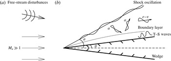
We consider a supersonic flow past a wedge with a semi-angle
 ${\it\theta}$
. The wedge is taken to be symmetrically aligned with the oncoming flow. A straight shock forms and makes an acute angle
 ${\it\sigma}$
with the symmetry line of the wedge as is illustrated in figure 1; the angle between the shock and the wedge surface is
 ${\it\phi}={\it\sigma}-{\it\theta}$
. The steady velocity, density, pressure and temperature are denoted by
 $\breve{u}$
,
 $\breve{{\it\rho}}$
,
 $\breve{p}$
and
 $\breve{T}$
respectively. Quantities upstream of the shock are indicated by the subscript ‘
 $u$
’, whereas those between the shock and wedge by the subscript ‘
 $s$
’. The oncoming flow has a mean speed
 $\breve{U}_{u}$
, and is perturbed by three-dimensional small-amplitude disturbances, which are to be specified shortly. The fluid is assumed to be a perfect gas with a constant ratio of specific heats
 ${\it\gamma}$
. Based upon
 $\breve{U}_{u}$
and the upstream sound speed
 $\breve{a}_{u}=\sqrt{{\it\gamma}\breve{p}_{u}/\breve{{\it\rho}}_{u}}$
, the upstream Mach number
 $M_{u}$
is defined as
 $$\begin{eqnarray}\displaystyle M_{u}=\breve{U}_{u}/\breve{a}_{u}. & & \displaystyle\end{eqnarray}$$
The uniform velocity, density, pressure, temperature, shear viscosity and sound speed between the shock and the wedge are denoted by
 $\breve{U}_{s}$
,
 $\breve{{\it\rho}}_{s}$
,
 $\breve{p}_{s}$
,
 $\breve{T}_{s}$
,
 $\breve{{\it\mu}}_{s}$
and
 $\breve{a}_{s}$
, respectively. Using these quantities, we define the Reynolds number
 $Re$
and the Mach number
 $M$
as
 $$\begin{eqnarray}\displaystyle Re=\breve{{\it\rho}}_{s}\breve{U}_{s}\breve{l}/\breve{{\it\mu}}_{s},\quad M=\breve{U}_{s}/\breve{a}_{s}, & & \displaystyle\end{eqnarray}$$
where
 $\breve{l}$
denotes the distance from the wedge tip to the location of interest.
Flow configuration and unsteady disturbances. The letters ‘a’, ‘
 $v$
’ and ‘e’ refer to acoustic, vortical and entropy perturbations respectively.

The inviscid solution for the steady flow relates the uniform quantities upstream and downstream the shock (e.g. see Hayes & Probstein Reference Hayes and Probstein2004). Specifically,
 $$\begin{eqnarray}\displaystyle {\it\epsilon}\equiv \frac{\breve{{\it\rho}}_{u}}{\breve{{\it\rho}}_{s}}=\left(\frac{{\it\gamma}-1}{{\it\gamma}+1}\right)\left(1+\frac{2}{({\it\gamma}-1)M_{u}^{2}\sin ^{2}{\it\sigma}}\right),\quad \frac{\breve{p}_{s}}{\breve{p}_{u}}=1+{\it\gamma}M_{u}^{2}\sin ^{2}{\it\sigma}(1-{\it\epsilon}), & & \displaystyle \nonumber\\ \displaystyle & & \displaystyle\end{eqnarray}$$
 $$\begin{eqnarray}\displaystyle \tan {\it\phi}={\it\epsilon}\tan {\it\sigma},\quad M^{2}=\frac{M_{u}^{2}\cos ^{2}{\it\sigma}(1+{\it\epsilon}^{2}\tan ^{2}{\it\sigma})}{1+\displaystyle \frac{1}{2}({\it\gamma}-1)(1-{\it\epsilon}^{2})M_{u}^{2}\sin ^{2}{\it\sigma}}. & & \displaystyle\end{eqnarray}$$
Two Cartesian coordinate systems will be used to describe different aspects of the flow. The interaction of unsteady disturbances with the shock will be analysed in the system oriented with the shock. The boundary-layer flow will be considered in the system
 $(x,y,z)$
with its origin at the wedge tip, where
 $x$
and
 $y$
are along and normal to the wedge surface, respectively, and
 $z$
is in the spanwise direction, all non-dimensionalized by
 $\breve{l}$
. The time variable
 $t$
is normalized by
 $\breve{l}/\breve{U}_{s}$
. The velocity
 $(u,v,w)$
, density
 ${\it\rho}$
, pressure
 $p$
, temperature
 $T$
and shear and bulk viscosities
 ${\it\mu}$
and
 ${\it\mu}^{\prime }$
are non-dimensionalized by
 $\breve{U}_{s}$
,
 $\breve{{\it\rho}}_{s}$
,
 $\breve{{\it\rho}}_{s}\breve{U}_{s}^{2}$
,
 $\breve{T}_{s}$
and
 $\breve{{\it\mu}}_{s}$
, respectively. The flow is governed by the compressible Navier–Stokes (N–S) equations,
 $$\begin{eqnarray}\displaystyle & \displaystyle \frac{\partial {\it\rho}}{\partial t}+\boldsymbol{{\rm\nabla}}\boldsymbol{\cdot }({\it\rho}\boldsymbol{u})=0, & \displaystyle\end{eqnarray}$$
 $$\begin{eqnarray}\displaystyle & \displaystyle {\it\rho}\frac{\text{D}\boldsymbol{u}}{\text{D}t}=-\boldsymbol{{\rm\nabla}}p+\frac{1}{Re}\left[\boldsymbol{{\rm\nabla}}\boldsymbol{\cdot }(2{\it\mu}\unicode[STIX]{x1D65A})+\boldsymbol{{\rm\nabla}}\left(\left({\it\mu}^{\prime }-\frac{2}{3}{\it\mu}\right)\boldsymbol{{\rm\nabla}}\boldsymbol{\cdot }\boldsymbol{u}\right)\right], & \displaystyle\end{eqnarray}$$
 $$\begin{eqnarray}\displaystyle & \displaystyle {\it\rho}\frac{\text{D}T}{\text{D}t}=({\it\gamma}-1)M^{2}\frac{\text{D}p}{\text{D}t}+\frac{1}{PrRe}\boldsymbol{{\rm\nabla}}\boldsymbol{\cdot }({\it\mu}\boldsymbol{{\rm\nabla}}T)+\frac{({\it\gamma}-1)M^{2}}{Re}{\it\Phi}, & \displaystyle\end{eqnarray}$$
 $$\begin{eqnarray}\displaystyle & \displaystyle {\it\gamma}M^{2}p={\it\rho}T, & \displaystyle\end{eqnarray}$$
 $\unicode[STIX]{x1D65A}$
and
 ${\it\Phi}$
denote the strain-rate tensor and the dissipation function respectively,
 $$\begin{eqnarray}\displaystyle \unicode[STIX]{x1D626}_{ij}=\frac{1}{2}\left(\frac{\partial u_{i}}{\partial x_{j}}+\frac{\partial u_{j}}{\partial x_{i}}\right),\quad {\it\Phi}=2{\it\mu}\unicode[STIX]{x1D65A}\boldsymbol{ : }\unicode[STIX]{x1D65A}+\left({\it\mu}^{\prime }-\frac{2}{3}{\it\mu}\right)(\boldsymbol{{\rm\nabla}}\boldsymbol{\cdot }\boldsymbol{u})^{2}, & & \displaystyle\end{eqnarray}$$
and
 $Pr$
is the Prandtl number. The dependence of the shear viscosity
 ${\it\mu}$
on the temperature is described by a viscosity law. For the present problem, the viscosity law does not affect the results qualitatively. For simplicity, we use the Chapman law, which can be written as
 ${\it\mu}=T$
for the normalization adopted. Furthermore we take
 ${\it\mu}^{\prime }=0$
.
2.1 The base flow
In the coordinate system
 $({\it\xi},{\it\eta},z)$
, the inviscid part of the base flow is given by Cowley & Hall (Reference Cowley and Hall1990)
 $$\begin{eqnarray}\displaystyle & \displaystyle \bar{R}={\it\epsilon},\quad R=1,\quad \bar{U}=U=\frac{1}{(1+{\it\epsilon}^{2}\mathscr{T}^{2})^{1/2}},\quad \bar{V}=-\frac{\mathscr{T}}{(1+{\it\epsilon}^{2}\mathscr{T}^{2})^{1/2}},\quad V={\it\epsilon}\bar{V}, & \displaystyle \nonumber\\ \displaystyle & & \displaystyle\end{eqnarray}$$
 $$\begin{eqnarray}\displaystyle & \displaystyle \bar{W}=W=0,\quad \bar{P}=\frac{{\it\epsilon}}{{\it\gamma}M^{2}}-\frac{{\it\epsilon}({\it\gamma}-1)(1-{\it\epsilon}^{2})\mathscr{T}^{2}}{2{\it\gamma}(1+{\it\epsilon}^{2}\mathscr{T}^{2})},\quad P=\frac{1}{{\it\gamma}M^{2}},\quad \mathscr{T}=\tan {\it\sigma}, & \displaystyle \nonumber\\ \displaystyle & & \displaystyle\end{eqnarray}$$
 $$\begin{eqnarray}\displaystyle & \displaystyle \bar{E}=\frac{\bar{P}}{({\it\gamma}-1)\bar{R}}+\frac{1}{2}(\bar{U}^{2}+\bar{V}^{2}),\quad E=\frac{P}{({\it\gamma}-1)R}+\frac{1}{2}(U^{2}+V^{2}), & \displaystyle\end{eqnarray}$$
The viscous boundary layer is described by the transverse variable
 $$\begin{eqnarray}\displaystyle {\tilde{Y}}=Re^{1/2}y, & & \displaystyle\end{eqnarray}$$
and its streamwise velocity profile is given by the similarity solution
 $$\begin{eqnarray}\displaystyle U_{B}=f^{\prime }({\it\zeta})\quad \text{with }{\it\zeta}=\frac{1}{\sqrt{x}}\int _{0}^{{\tilde{Y}}}R_{B}\,\text{d}{\tilde{Y}}, & & \displaystyle\end{eqnarray}$$
where
 $R_{B}$
in
 ${\it\zeta}$
(the Dorodnitsyn–Howarth variable) is the mean density profile. It can be shown that
 $$\begin{eqnarray}\displaystyle U_{B}\rightarrow {\it\lambda}{\it\mu}_{w}^{-1/2}T_{w}^{-1/2}{\tilde{Y}}\quad \text{as }{\tilde{Y}}\rightarrow 0, & & \displaystyle\end{eqnarray}$$
where
 ${\it\lambda}={\it\chi}x^{-1/2}$
with
 ${\it\chi}\approx 0.332$
, while
 ${\it\mu}_{w}$
and
 $T_{w}$
denote the shear viscosity and temperature on the wall, respectively; for the Chapman law,
 ${\it\mu}_{w}=T_{w}$
. For simplicity, we assume that (1) the wedge walls are insulating, i.e.
 $\partial T_{B}/\partial {\tilde{Y}}=0$
on
 ${\tilde{Y}}=0$
and (2) the Prandtl number is unity, i.e.
 $Pr=1$
. Then the temperature and density of the boundary-layer flow,
 $T_{B}$
and
 $R_{B}$
, are given by
 $$\begin{eqnarray}\displaystyle T_{B}=1+\frac{{\it\gamma}-1}{2}M^{2}(1-U_{B}^{2}),\quad R_{B}=T_{B}^{-1}. & & \displaystyle\end{eqnarray}$$
2.2 Unsteady disturbances
Upstream of the shock, an unsteady perturbation with a small amplitude of order
 ${\it\delta}\ll 1$
is superimposed on the steady flow. In order to derive the so-called shock condition satisfied by the disturbance downstream of the shock, it is convenient to work with the coordinate system
 $({\it\xi},{\it\eta},z)$
, where
 ${\it\xi}$
,
 ${\it\eta}$
are parallel and normal to the shock, respectively, and
 $z$
is in the spanwise direction; they are normalized by
 $\breve{l}$
, the distance to the leading edge. The corresponding velocity field is denoted by
 $(u,v,w)$
. The total flow field can be written as
 $$\begin{eqnarray}\displaystyle ({\it\rho},u,v,w,p,\mathscr{E})=(\bar{R},\bar{U},\bar{V},0,\bar{P},\bar{E})+{\it\delta}(\tilde{r}_{0},\tilde{u} _{0},\tilde{v}_{0},\tilde{w}_{0},\tilde{p}_{0},\tilde{e}_{0}), & & \displaystyle\end{eqnarray}$$
where
 $\mathscr{E}=p/[({\it\gamma}-1){\it\rho}]+(u^{2}+v^{2}+w^{2})/2$
.
As the background flow is uniform, the perturbation can be decomposed as
 $$\begin{eqnarray}\displaystyle & \displaystyle \tilde{e}_{0}=\frac{1}{({\it\gamma}-1)\bar{R}}\tilde{p}_{0}-\frac{\bar{P}}{({\it\gamma}-1)\bar{R}^{2}}\tilde{r}_{0}+\bar{U}\tilde{u} _{0}+\bar{V}\tilde{v}_{0}, & \displaystyle\end{eqnarray}$$
 $$\begin{eqnarray}\displaystyle & \displaystyle \tilde{u} _{0}=\tilde{u} _{0a}^{+}+\tilde{u} _{0a}^{-}+\tilde{u} _{0v},\quad \tilde{v}_{0}=\tilde{v}_{0a}^{+}+\tilde{v}_{0a}^{-}+\tilde{v}_{0v},\quad \tilde{w}_{0}=\tilde{w}_{0a}^{+}+\tilde{w}_{0a}^{-}+\tilde{w}_{0v}, & \displaystyle\end{eqnarray}$$
 $$\begin{eqnarray}\displaystyle & \displaystyle \tilde{p}_{0}=\tilde{p}_{0a}^{+}+\tilde{p}_{0a}^{-},\quad \tilde{r}_{0}=\tilde{r}_{0a}^{+}+\tilde{r}_{0a}^{-}+\tilde{r}_{0e}, & \displaystyle\end{eqnarray}$$
 $a$
’, ‘
 $v$
’ and ‘
 $e$
’ indicate acoustic, vorticity and entropy modes respectively with the sign ‘
 $+/-$
’ referring to fast/slow acoustic waves respectively.
Each of three types of perturbations is governed by the linearized N–S equations about the uniform mean field. Acoustic waves are irrotational, and their pressure, density and velocity are found as
 $$\begin{eqnarray}\displaystyle \left.\begin{array}{@{}c@{}}\displaystyle \tilde{p}_{0a}^{\pm }=p_{I}^{\pm }\text{e}^{\text{i}{\it\nu}_{0}^{\pm }{\it\eta}}\tilde{E}_{0}+\text{c.c.},\quad \tilde{r}_{0a}^{\pm }=M_{u}^{2}\frac{\cos ^{2}{\it\sigma}}{\cos ^{2}{\it\phi}}p_{I}^{\pm }\text{e}^{\text{i}{\it\nu}_{0}^{\pm }{\it\eta}}\tilde{E}_{0}+\text{c.c.},\\ \displaystyle (\tilde{u} _{0a}^{\pm },\tilde{v}_{0a}^{\pm },\tilde{w}_{0a}^{\pm })=({\it\alpha},{\it\nu}_{0}^{\pm },{\it\beta})\frac{p_{I}^{\pm }}{({\it\omega}-{\it\alpha}\bar{U}-{\it\nu}_{0}^{\pm }\bar{V})\bar{R}}\text{e}^{\text{i}{\it\nu}_{0}^{\pm }{\it\eta}}\tilde{E}_{0}+\text{c.c.},\end{array}\right\} & & \displaystyle\end{eqnarray}$$
where we have introduced
 $$\begin{eqnarray}\displaystyle \tilde{E}_{0}=\text{e}^{\text{i}({\it\alpha}{\it\xi}+{\it\beta}z-{\it\omega}t)}, & & \displaystyle\end{eqnarray}$$
and the frequency and wavenumbers satisfy the acoustic dispersion relation
 $$\begin{eqnarray}\displaystyle {\it\omega}-{\it\alpha}\bar{U}-{\it\nu}_{0}^{\pm }\bar{V}=\pm \frac{\cos {\it\phi}}{M_{u}\cos {\it\sigma}}\sqrt{{\it\alpha}^{2}+({\it\nu}_{0}^{\pm })^{2}+{\it\beta}^{2}}. & & \displaystyle\end{eqnarray}$$
A vorticity wave has, on the other hand, no pressure fluctuation, and its velocity components take the form
 $$\begin{eqnarray}\displaystyle (\tilde{u} _{0v},\tilde{v}_{0v},\tilde{w}_{0v})=(u_{I},v_{I},w_{I})\text{e}^{\text{i}{\it\nu}_{I}{\it\eta}}\tilde{E}_{0}+\text{c.c.}, & & \displaystyle\end{eqnarray}$$
whereas an entropy mode carries merely a density (or temperature) fluctuation,
 $$\begin{eqnarray}\displaystyle \tilde{r}_{0e}=r_{I}\text{e}^{\text{i}{\it\nu}_{I}{\it\eta}}\tilde{E}_{0}+\text{c.c.} & & \displaystyle\end{eqnarray}$$
For both vorticity and entropy modes, the wavenumber in the
 ${\it\eta}$
-direction,
 ${\it\nu}_{I}$
, satisfies the dispersion relation
 $$\begin{eqnarray}\displaystyle {\it\omega}-{\it\alpha}\bar{U}-{\it\nu}_{I}\bar{V}=0. & & \displaystyle\end{eqnarray}$$
In general, whenever any one of acoustic, vorticity and entropy waves strikes a shock, all three types of fluctuations may arise altogether downstream. They will be referred to as transmitted waves if they are of the same type as the upstream ones, or generated waves if different. The generated/transmitted waves have the same frequency and the same wavelengths parallel to the shock as the disturbance upstream. For a shock in free space, the disturbances downstream are all transmitted from, and/or generated by, the upstream perturbation. However, for a shock adjacent to a wall, along which a boundary layer develops, there may also exist the free-stream signature of boundary-layer instability modes. This is the case for the present problem. We shall assume that the perturbation has a short wavelength, i.e.
 ${\it\alpha},{\it\beta}\gg 1$
. The perturbation downstream the shock is allowed to modulate slowly over a length scale much longer than
 $2{\rm\pi}/{\it\alpha}$
but much shorter than
 $O(1)$
. The modulation is described by the variable
 $x_{1}=x/\tilde{{\it\epsilon}}$
, where
 $2{\rm\pi}/{\it\alpha}\leqslant \tilde{{\it\epsilon}}^{2}\ll 1$
. With the above considerations, we write the downstream flow field as
 $$\begin{eqnarray}\displaystyle ({\it\rho},u,v,w,p,\mathscr{E}) & = & \displaystyle (R,U,V,0,P,E)+{\it\delta}\tilde{{\it\epsilon}}^{-1} [(\tilde{r}_{1},\tilde{u} _{1},\tilde{v}_{1},\tilde{w}_{1},\tilde{p}_{1},\tilde{e}_{1})\nonumber\\ \displaystyle & & \displaystyle +\,\tilde{{\it\epsilon}}(\tilde{r}_{2},\tilde{u} _{2},\tilde{v}_{2},\tilde{w}_{2},\tilde{p}_{2},\tilde{e}_{2})],\end{eqnarray}$$
where the
 $O({\it\delta}/\tilde{{\it\epsilon}})$
term represents the signature of the T–S wave that may be generated by the
 $O({\it\delta})$
disturbance in the oncoming flow. The larger magnitude is due to the resonant nature of the forcing. This term is present in the expansion near the neutral position of the T–S wave, but would be absent upstream of the neutral position. The disturbance in (2.20) again consists of acoustic, vortical and entropy parts, namely
 $$\begin{eqnarray}\displaystyle & \displaystyle \tilde{e}_{j}=\frac{1}{({\it\gamma}-1)R}\tilde{p}_{j}-\frac{P}{({\it\gamma}-1)R^{2}}\tilde{r}_{j}+U\tilde{u} _{j}+V\tilde{v}_{j}, & \displaystyle\end{eqnarray}$$
 $$\begin{eqnarray}\displaystyle & \displaystyle \tilde{u} _{j}=\tilde{u} _{ja}+\tilde{u} _{jv},\quad \tilde{v}_{j}=\tilde{v}_{ja}+\tilde{v}_{jv},\quad \tilde{w}_{j}=\tilde{w}_{ja}+\tilde{w}_{jv}, & \displaystyle\end{eqnarray}$$
 $$\begin{eqnarray}\displaystyle & \displaystyle \tilde{p}_{j}=\tilde{p}_{ja},\quad \quad \tilde{r}_{j}=\tilde{r}_{ja}+\tilde{r}_{je},\quad (j=1,2). & \displaystyle\end{eqnarray}$$
The leading-order (i.e.
 $O({\it\delta}\tilde{{\it\epsilon}}^{-1})$
) acoustic part admits the solution for the pressure
 $$\begin{eqnarray}\displaystyle \tilde{p}_{1a}=({\check{a}}_{I}\text{e}^{\text{i}{\it\nu}_{1}{\it\eta}}+{\check{a}}_{R}\text{e}^{\text{i}{\it\nu}_{2}{\it\eta}})\tilde{E}_{0}, & & \displaystyle\end{eqnarray}$$
where
 ${\it\nu}_{1}$
and
 ${\it\nu}_{2}$
are the wavenumbers of the incoming and outgoing slow acoustic waves, and they satisfy the dispersion relation
 $$\begin{eqnarray}\displaystyle {\it\omega}-{\it\alpha}U-{\it\nu}_{1,2}V=-\frac{1}{M}\sqrt{{\it\alpha}^{2}+{\it\nu}_{1,2}^{2}+{\it\beta}^{2}}, & & \displaystyle\end{eqnarray}$$
and the amplitudes of these two waves,
 ${\check{a}}_{I}$
and
 ${\check{a}}_{R}$
, are functions of
 $x_{1}$
. Note that a minus sign on the right-hand side of (2.23) is taken because a T–S instability mode has a small phase speed, and behaves outside the boundary layer like a slow acoustic wave. The corresponding expressions for the velocities and the solution for the induced vortical part of the disturbance are given in appendix A. The result will be used in the main text specifically for
 ${\it\alpha}=O(Re^{3/8}{\it\mu}_{w}^{-3/8}T_{w}^{-9/8}M^{-3/4})$
,
 ${\it\beta}=O(Re^{3/8}{\it\mu}_{w}^{-3/8}T_{w}^{-9/8}M^{1/4})$
and
 $\tilde{{\it\epsilon}}=Re^{-3/16}{\it\mu}_{w}^{3/16}T_{w}^{9/16}M^{3/8}$
.
The
 $O({\it\delta})$
disturbance downstream the shock consists of two parts: (i) that transmitted from, or generated by, the upstream perturbation and (ii) that arising from the modulation of the leading-order (i.e.
 $O({\it\delta}/\tilde{{\it\epsilon}})$
) fluctuations associated with the T–S mode. The solution for the acoustic part, which is governed by the inhomogeneous wave equation, is of the form
 $$\begin{eqnarray}\displaystyle \tilde{p}_{2a}=(\hat{a}_{I}\text{e}^{\text{i}{\it\nu}_{1}{\it\eta}}+\hat{a}_{R}\text{e}^{\text{i}{\it\nu}_{2}{\it\eta}}+\hat{p}_{2a,p})\tilde{E}_{0}, & & \displaystyle\end{eqnarray}$$
where
 $\hat{p}_{2a,p}$
denotes the particular solution and
 $\hat{a}_{I}$
and
 $\hat{a}_{R}$
are functions of
 $x_{1}$
.
For an oblique shock in free space, the relations satisfied by the disturbance on the shock were given by McKenzie & Westphal (Reference McKenzie and Westphal1968). In the presence of a wall, the analysis must allow for the acoustic wave reflected by the wall as well as for the signature of the boundary-layer perturbations. These were considered by Cowley & Hall (Reference Cowley and Hall1990) but the upstream disturbance was assumed absent. Here, we consider the case where the upstream disturbance may be comprised of any of three types of modes. Furthermore, the disturbance downstream may be spatially modulated. The detailed analysis of their interaction with a general oblique shock is performed by Qin & Wu (Reference Qin and Wu2016) for any
 $\tilde{{\it\epsilon}}$
satisfying
 $2{\rm\pi}/{\it\alpha}\leqslant \tilde{{\it\epsilon}}^{2}\ll 1$
, and the generalized shock conditions are derived. In appendix A, these conditions are specialized to (2.7a–c
), leading to (A 7) and (A 21), which relate
 ${\check{a}}_{I}$
and
 ${\check{a}}_{R}$
in (2.22), and
 $\hat{a}_{I}$
and
 $\hat{a}_{R}$
in (2.24), respectively. The relations (A 7) and (A 21) simplify significantly for disturbances on the triple-deck scales.
In the coordinate system
 $(x,y,z)$
, the leading-order pressure
 $\tilde{p}$
is governed by
 $$\begin{eqnarray}\displaystyle M^{2}\left(\frac{\partial }{\partial t}+\frac{\partial }{\partial x}\right)^{2}\tilde{p}-{\rm\nabla}^{2}\tilde{p}=0. & & \displaystyle\end{eqnarray}$$
The solution takes the form
 $$\begin{eqnarray}\displaystyle \tilde{p}={\it\delta}[a_{I}\text{e}^{\text{i}({\it\alpha}_{a}x+{\it\gamma}_{a}y+{\it\beta}_{a}z-{\it\omega}_{a}t)}+a_{R}\text{e}^{\text{i}({\it\alpha}_{a}x-{\it\gamma}_{a}y+{\it\beta}_{a}z-{\it\omega}_{a}t)}]. & & \displaystyle\end{eqnarray}$$
Substitution of (2.26) into (2.25) leads to the dispersion relation for slow acoustic waves,
 $$\begin{eqnarray}\displaystyle {\it\omega}_{a}/{\it\alpha}_{a}=1-\frac{1}{M}\sqrt{1+({\it\beta}_{a}/{\it\alpha}_{a})^{2}+({\it\gamma}_{a}/{\it\alpha}_{a})^{2}}. & & \displaystyle\end{eqnarray}$$
Note that the two coordinate systems,
 $(x,y,z)$
and
 $({\it\xi},{\it\eta},z)$
, are related to each other by
 $$\begin{eqnarray}\displaystyle x={\it\xi}\cos {\it\phi}-{\it\eta}\sin {\it\phi},\quad y={\it\xi}\sin {\it\phi}+{\it\eta}\cos {\it\phi}. & & \displaystyle\end{eqnarray}$$
The wavenumbers in the two systems are related by
 $$\begin{eqnarray}\displaystyle {\it\alpha}_{a}={\it\alpha}\cos {\it\phi}-{\it\nu}_{1,2}\sin {\it\phi},\quad {\it\gamma}_{a}={\it\alpha}\sin {\it\phi}+{\it\nu}_{1,2}\cos {\it\phi}, & & \displaystyle\end{eqnarray}$$
with which the dispersion relations (2.23) and (2.27) are equivalent as expected. When
 ${\it\phi}\ll 1$
, which is the case for our problem, the expressions (2.22) and (2.26) are identical on the shock (
 ${\it\eta}=0$
) provided that
 $$\begin{eqnarray}\displaystyle {\check{a}}_{I}=a_{I}\text{e}^{\text{i}{\it\gamma}_{a}y_{s}},\quad {\check{a}}_{R}=a_{R}\text{e}^{-\text{i}{\it\gamma}_{a}y_{s}}, & & \displaystyle\end{eqnarray}$$
where
 $y_{s}={\it\xi}\sin {\it\phi}=x\tan {\it\phi}$
is the local shock position.
2.3 Asymptotic scalings
In order to develop an asymptotic theory for receptivity, we assume the Reynolds and Mach numbers to be large:
 $Re\gg 1$
and
 $M\gg 1$
. More specifically, for the base flow we adopt the same scaling restrictions as those in Cowley & Hall (Reference Cowley and Hall1990),
 $$\begin{eqnarray}\displaystyle {\it\sigma}\ll 1,\quad M\gg 1,\quad {\it\sigma}M\gg 1,\quad {\it\epsilon}\approx 1/({\it\sigma}^{2}M^{2}),\quad {\it\gamma}-1\sim \bar{{\it\gamma}}/({\it\sigma}^{2}M^{2}),\qquad & & \displaystyle\end{eqnarray}$$
to ensure that the shock is sufficiently close to the wall to influence the boundary-layer instability. Use of (2.31) to the first equation in (2.3a,b ) shows that
 $$\begin{eqnarray}\displaystyle M_{u}^{2}=\frac{2}{\sin ^{2}{\it\sigma}[({\it\gamma}+1){\it\epsilon}-{\it\gamma}+1]}\sim \frac{2}{2-\bar{{\it\gamma}}}M^{2}, & & \displaystyle\end{eqnarray}$$
where
 $\bar{{\it\gamma}}$
is an
 $O(1)$
constant and
 $0<\bar{{\it\gamma}}<2$
.
In the limit of
 $Re\gg 1$
and
 $M\gg 1$
, the characteristic frequency of lower-branch T–S waves,
 ${\it\omega}_{TS}$
, and their wavenumbers in the
 $x$
- and
 $z$
-directions,
 ${\it\alpha}_{TS}$
and
 ${\it\beta}_{TS}$
, scale as (Smith Reference Smith1989; Cowley & Hall Reference Cowley and Hall1990)
 $$\begin{eqnarray}\displaystyle {\it\omega}_{TS}=Re^{1/4}{\it\mu}_{w}^{-1/4}T_{w}^{-3/4}M^{-1/2}\hat{{\it\omega}}_{TS},\quad ({\it\alpha}_{TS},{\it\beta}_{TS})=Re^{3/8}{\it\mu}_{w}^{-3/8}T_{w}^{-9/8}M^{-3/4}(\hat{{\it\alpha}}_{TS},M\hat{{\it\beta}}_{TS}). & & \displaystyle \nonumber\\ \displaystyle & & \displaystyle\end{eqnarray}$$
The disturbance in the oncoming free stream is in general of broadband nature and so are those emerging downstream of the shock, among which each acoustic wave is characterized by its frequency
 ${\it\omega}_{a}$
, and streamwise and spanwise wavenumbers,
 ${\it\alpha}_{a}$
and
 ${\it\beta}_{a}$
(with
 ${\it\gamma}_{a}$
determined by the dispersion relation (2.27)). Our interest is in Fourier components which generate T–S waves. This requires
 ${\it\omega}_{a}$
,
 ${\it\alpha}_{a}$
and
 ${\it\beta}_{a}$
of slow acoustic waves to be on the same triple-deck scales,
 $$\begin{eqnarray}\displaystyle {\it\omega}_{a}=Re^{1/4}{\it\mu}_{w}^{-1/4}T_{w}^{-3/4}M^{-1/2}\hat{{\it\omega}}_{a},\quad ({\it\alpha}_{a},{\it\beta}_{a})=Re^{3/8}{\it\mu}_{w}^{-3/8}T_{w}^{-9/8}M^{-3/4}(\hat{{\it\alpha}}_{a},M\hat{{\it\beta}}_{a}). & & \displaystyle \nonumber\\ \displaystyle & & \displaystyle\end{eqnarray}$$
Substitution of the scalings (2.34) into (2.27) leads to
 $$\begin{eqnarray}\displaystyle 1-\frac{1}{M}\sqrt{1+(\hat{{\it\beta}}_{a}/\hat{{\it\alpha}}_{a})^{2}M^{2}+({\it\gamma}_{a}/{\it\alpha}_{a})^{2}}=Re^{-1/8}{\it\mu}_{w}^{1/8}T_{w}^{3/8}M^{1/4}(\hat{{\it\omega}}_{a}/\hat{{\it\alpha}}_{a}). & & \displaystyle\end{eqnarray}$$
In order for the left-hand side of the equation to be positive and asymptotically small, we require that
 $\hat{{\it\alpha}}_{a}>\hat{{\it\beta}}_{a}$
and
 ${\it\gamma}_{a}=Re^{3/8}{\it\mu}_{w}^{-3/8}T_{w}^{-9/8}M^{1/4}\hat{{\it\gamma}}_{a}$
with
 $\hat{{\it\gamma}}_{a}$
being given, to leading order, by
 $$\begin{eqnarray}\displaystyle \hat{{\it\gamma}}_{a}=\sqrt{\hat{{\it\alpha}}_{a}^{2}-\hat{{\it\beta}}_{a}^{2}}. & & \displaystyle\end{eqnarray}$$
This relation specifies the propagation direction of the slow acoustic waves which have wavelengths and phase speeds comparable with those of T–S waves. Consistent with the scalings (2.34), we introduce the time, the streamwise and spanwise variables
 $$\begin{eqnarray}\displaystyle \bar{t}=Re^{1/4}{\it\mu}_{w}^{-1/4}T_{w}^{-3/4}M^{-1/2}t,\quad (\bar{x},\bar{z})=Re^{3/8}{\it\mu}_{w}^{-3/8}T_{w}^{-9/8}M^{-3/4}(x,Mz). & & \displaystyle\end{eqnarray}$$
In order for a slow acoustic wave on the scales (2.34) to arise downstream, upstream (fast or slow) acoustic, vortical and entropy modes must have appropriate scales. For all these modes, the wavenumber parallel to the shock
 $$\begin{eqnarray}\displaystyle {\it\alpha}\approx {\it\alpha}_{a}=Re^{3/8}{\it\mu}_{w}^{-3/8}T_{w}^{-9/8}M^{-3/4}\hat{{\it\alpha}}_{a}, & & \displaystyle\end{eqnarray}$$
but that normal to the shock is different. For a fast/slow upstream acoustic mode, it follows from (2.16) and (2.32) that to leading-order accuracy,
 $$\begin{eqnarray}\displaystyle {\it\nu}_{0}^{\pm }\approx Re^{3/8}{\it\mu}_{w}^{-3/8}T_{w}^{-9/8}M^{-3/4}\left.\left(\hat{{\it\alpha}}_{a}\pm \sqrt{\frac{2-\bar{{\it\gamma}}}{2}}\hat{{\it\beta}}_{a}\right)\!\right/\!{\it\sigma}. & & \displaystyle\end{eqnarray}$$
For upstream vorticity and entropy modes, we find from (2.19) that
 $$\begin{eqnarray}\displaystyle {\it\nu}_{I}\approx Re^{3/8}{\it\mu}_{w}^{-3/8}T_{w}^{-9/8}M^{-3/4}\hat{{\it\alpha}}_{a}/{\it\sigma}. & & \displaystyle\end{eqnarray}$$
At a general streamwise location
 $x$
where
 $({\it\omega}_{a},{\it\alpha}_{a},{\it\beta}_{a})\neq ({\it\omega}_{TS},{\it\alpha}_{TS},{\it\beta}_{TS})$
, an acoustic wave generates a finite response within the boundary layer. However, for each frequency
 ${\it\omega}_{a}$
, there exists a location
 $x_{0}$
at which a T–S wave with the same frequency and spanwise wavenumber is neutrally stable if the streamwise wavenumber of the slow acoustic wave also coincides with that of the neutral T–S mode, that is,
 $$\begin{eqnarray}\displaystyle \hat{{\it\omega}}_{a}=\hat{{\it\omega}}_{TS},\quad \hat{{\it\alpha}}_{a}=\hat{{\it\alpha}}_{TS},\quad \hat{{\it\beta}}_{a}=\hat{{\it\beta}}_{TS} & & \displaystyle\end{eqnarray}$$
at
 $x_{0}$
, the response becomes unbounded, signalling that a resonance takes place in the vicinity of
 $x_{0}$
. A scaling argument similar to that of Wu (Reference Wu2001b
) shows that the forced response evolves into a T–S mode under the influence of non-parallelism, and this resonance region corresponds to
 $x-x_{0}=O(\bar{{\it\epsilon}})$
with
 $$\begin{eqnarray}\displaystyle \bar{{\it\epsilon}}=Re^{-3/16}{\it\mu}_{w}^{3/16}T_{w}^{9/16}M^{3/8}. & & \displaystyle\end{eqnarray}$$
In order to describe the evolution of the disturbance through the resonance region, we introduce
 $$\begin{eqnarray}\displaystyle x_{1}=(x-x_{0})/\bar{{\it\epsilon}}. & & \displaystyle\end{eqnarray}$$
It follows from (2.37) and (2.43) that
 $$\begin{eqnarray}\displaystyle \frac{\partial }{\partial t}\rightarrow Re^{1/4}{\it\mu}_{w}^{-1/4}T_{w}^{-3/4}M^{-1/2}\frac{\partial }{\partial \bar{t}},\quad \frac{\partial }{\partial z}\rightarrow \bar{{\it\epsilon}}^{-2}M\frac{\partial }{\partial \bar{z}},\quad \frac{\partial }{\partial x}\rightarrow \bar{{\it\epsilon}}^{-2}\left(\frac{\partial }{\partial \bar{x}}+\bar{{\it\epsilon}}\frac{\partial }{\partial x_{1}}\right). & & \displaystyle \nonumber\\ \displaystyle & & \displaystyle\end{eqnarray}$$
We further expand
 ${\it\lambda}$
about
 $x_{0}$
,
 $$\begin{eqnarray}\displaystyle {\it\lambda}={\it\lambda}_{0}+\bar{{\it\epsilon}}{\it\lambda}_{1}x_{1}\quad \text{with }{\it\lambda}_{1}=-{\textstyle \frac{1}{2}}{\it\chi}{x_{0}}^{-3/2}. & & \displaystyle\end{eqnarray}$$
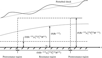
The asymptotic structure describing the boundary-layer response and receptivity is shown in figure 2. To a sound wave with its frequency and wavenumbers being scaled as (2.34), the boundary-layer response acquires, in the wall-normal direction, the triple-deck structure that governs the inherent boundary-layer instability. A disturbance satisfying the resonance condition (2.41) evolves, in the streamwise direction, through the pre-resonance, resonance and post-resonance regimes. The response in the pre-resonance regime will be considered in the next section, and the main result is the expressions (3.21) for
 $a_{I}$
and
 $a_{R}$
, the magnitudes of the pressure waves entering, and reflected by, the boundary layer, respectively. The evolution in the resonance region will be analysed in § 4 and the main outcome is (4.43), which describes the development of the response into a T–S wave, and allows us to determine the initial amplitude of the eigenmode excited.
The asymptotic structure of the boundary-layer response and receptivity.

3 Pre-resonance region: boundary-layer response to free-stream disturbances
For acoustic waves with wavelength comparable with the boundary-layer thickness, the response is essentially inviscid, and can be predicted by using the Rayleigh equation. However, for acoustic waves with long wavelengths and low frequencies, as specified by (2.34), the response is viscous and is described by triple-deck theory.
3.1 Upper deck
In the upper deck, the transverse variable is
 $$\begin{eqnarray}\displaystyle \bar{y}=Re^{3/8}{\it\mu}_{w}^{-3/8}T_{w}^{-9/8}M^{1/4}y, & & \displaystyle\end{eqnarray}$$
and the expansion takes the form
 $$\begin{eqnarray}\displaystyle (u,v,w,p,{\it\rho},T)=(1,0,0,1/{\it\gamma}M^{2},1,1)+{\it\delta}(u_{a},Mv_{a},Mw_{a},p_{a},M^{2}{\it\rho}_{a},M^{2}{\it\tau}_{a})+\cdots \,. & & \displaystyle \nonumber\\ \displaystyle & & \displaystyle\end{eqnarray}$$
Here we assume that there is no pre-existing T–S wave. In the pre-resonance region, no T–S wave is excited yet and so the
 $O({\it\delta}/\bar{{\it\epsilon}})$
term is absent. The perturbation is solely induced by the
 $O({\it\delta})$
disturbance in the oncoming flow.
We focus on the acoustic part of the perturbation. Vortical and entropy waves are also present (see appendix A), but they are absorbed by a thin layer located at the outer edge of the boundary layer without entering the latter (Dong & Wu Reference Dong and Wu2013; see also Maslov et al.
Reference Maslov, Mironov, Kudryavtsev, Poplavskaya and Tsyryulnokov2010, where such features were observed experimentally). The acoustic wave is governed by the (quasi-steady) Euler equations linearized about the uniform flow, among which the momentum equation in the
 $y$
-direction reads
 $$\begin{eqnarray}\displaystyle \frac{\partial v_{a}}{\partial \bar{x}}=-\frac{\partial p_{a}}{\partial \bar{y}}. & & \displaystyle\end{eqnarray}$$
The linearized Euler equations can be reduced to a single equation for
 $p_{a}$
,
 $$\begin{eqnarray}\displaystyle \frac{\partial ^{2}p_{a}}{\partial \bar{y}^{2}}-\frac{\partial ^{2}p_{a}}{\partial \bar{x}^{2}}+\frac{\partial ^{2}p_{a}}{\partial \bar{z}^{2}}=0. & & \displaystyle\end{eqnarray}$$
Equations (3.4) and (3.3) can be solved in sequence to find the solution for
 $p_{a}$
and
 $v_{a}$
,
 $$\begin{eqnarray}\displaystyle p_{a}=(a_{I}\text{e}^{\text{i}\hat{{\it\gamma}}_{a}\bar{y}}+a_{R}\text{e}^{-\text{i}\hat{{\it\gamma}}_{a}\bar{y}})E_{a}+\text{c.c.},\quad v_{a}=-\frac{\hat{{\it\gamma}}_{a}}{\hat{{\it\alpha}}_{a}}(a_{I}\text{e}^{\text{i}\hat{{\it\gamma}}_{a}\bar{y}}-a_{R}\text{e}^{-\text{i}\hat{{\it\gamma}}_{a}\bar{y}})E_{a}+\text{c.c.}, & & \displaystyle \nonumber\\ \displaystyle & & \displaystyle\end{eqnarray}$$
where
 $E_{a}=\exp \{\text{i}(\hat{{\it\alpha}}_{a}\bar{x}+\hat{{\it\beta}}_{a}\bar{z}-\hat{{\it\omega}}_{a}\bar{t})\}$
, and
 $a_{I}$
and
 $a_{R}$
depend on
 $x$
parametrically, and they represent respectively the amplitudes of the sound waves propagating towards and away from the wall. As
 $\bar{y}\rightarrow 0$
,
 $$\begin{eqnarray}\displaystyle p_{a}\rightarrow (a_{I}+a_{R})E_{a}+\text{c.c.},\quad v_{a}\rightarrow -\frac{\hat{{\it\gamma}}_{a}}{\hat{{\it\alpha}}_{a}}(a_{I}-a_{R})E_{a}+\text{c.c.} & & \displaystyle\end{eqnarray}$$
In the pre-resonance stage, the T–S signature is absent and thus the shock condition corresponds to (A 21) with the modulation terms being set to zero, which further reduces, for the disturbance on the triple-deck scales, to (A 46). Noting that
 $\hat{a}_{I}=a_{I}\text{e}^{\text{i}\hat{{\it\gamma}}_{a}\bar{y}_{s}}$
and
 $\hat{a}_{R}=a_{R}\text{e}^{-\text{i}\hat{{\it\gamma}}_{a}\bar{y}_{s}}$
(which are similar to (2.30)), we obtain
 $$\begin{eqnarray}\displaystyle a_{I}\text{e}^{\text{i}\hat{{\it\gamma}}_{a}\bar{y}_{s}}+a_{R}\text{e}^{-\text{i}\hat{{\it\gamma}}_{a}\bar{y}_{s}}=J_{0}, & & \displaystyle\end{eqnarray}$$
where
 $\bar{y}_{s}=Re^{3/8}{\it\mu}_{w}^{-3/8}T_{w}^{-9/8}M^{1/4}y_{s}$
is the rescaled shock position, and
 $J_{0}$
is defined in (A 47).
3.2 Main deck
In the main deck, the expansion takes the form
 $$\begin{eqnarray}\displaystyle & \displaystyle u=U_{B}({\tilde{Y}})+{\it\delta}Re^{1/8}{\it\mu}_{w}^{3/8}T_{w}^{9/8}M^{7/4}B_{a}U_{B}^{\prime }({\tilde{Y}})E_{a}+\text{c.c.}+\cdots \,, & \displaystyle\end{eqnarray}$$
 $$\begin{eqnarray}\displaystyle & \displaystyle v=-{\it\delta}M\text{i}\hat{{\it\alpha}}_{a}B_{a}U_{B}({\tilde{Y}})E_{a}+\text{c.c.}+\cdots \,, & \displaystyle\end{eqnarray}$$
where
 $B_{a}=B_{a}(x)$
depends on
 $x$
parametrically. It can be shown that
 $$\begin{eqnarray}\displaystyle & \displaystyle u\rightarrow {\it\lambda}{\it\mu}_{w}^{-1/2}T_{w}^{-1/2}{\tilde{Y}}+{\it\delta}Re^{1/8}{\it\mu}_{w}^{-1/8}T_{w}^{5/8}M^{7/4}B_{a}{\it\lambda}E_{a}+\text{c.c.}\quad \text{as }{\tilde{Y}}\rightarrow 0, & \displaystyle\end{eqnarray}$$
 $$\begin{eqnarray}\displaystyle & \displaystyle v\rightarrow -{\it\delta}M\text{i}\hat{{\it\alpha}}_{a}B_{a}E_{a}+\text{c.c.}\quad \text{as }{\tilde{Y}}\rightarrow \infty . & \displaystyle\end{eqnarray}$$
Matching with the normal velocity at the bottom of the upper deck, as given in (3.6), yields
 $$\begin{eqnarray}\displaystyle \frac{\hat{{\it\gamma}}_{a}}{\hat{{\it\alpha}}_{a}}(a_{I}-a_{R})=\text{i}\hat{{\it\alpha}}_{a}B_{a}. & & \displaystyle\end{eqnarray}$$
3.3 Lower deck
In the lower deck, the appropriate transverse coordinate is defined as
 $$\begin{eqnarray}\displaystyle Y=Re^{5/8}{\it\mu}_{w}^{-5/8}T_{w}^{-7/8}M^{-1/4}y, & & \displaystyle\end{eqnarray}$$
and the solution can be written as
 $$\begin{eqnarray}\displaystyle & \displaystyle u=Re^{-1/8}{\it\mu}_{w}^{1/8}T_{w}^{3/8}M^{1/4}{\it\lambda}Y+{\it\delta}Re^{1/8}{\it\mu}_{w}^{-1/8}T_{w}^{5/8}M^{7/4}\tilde{U} _{a}E_{a}+\text{c.c.}+\cdots \,, & \displaystyle\end{eqnarray}$$
 $$\begin{eqnarray}\displaystyle & \displaystyle v={\it\delta}Re^{-1/8}{\it\mu}_{w}^{1/8}T_{w}^{3/8}M^{5/4}\tilde{V}_{a}E_{a}+\text{c.c.}+\cdots \,, & \displaystyle\end{eqnarray}$$
 $$\begin{eqnarray}\displaystyle & \displaystyle w={\it\delta}Re^{1/8}{\it\mu}_{w}^{-1/8}T_{w}^{5/8}M^{3/4}\tilde{W}_{a}E_{a}+\text{c.c.}+\cdots \,, & \displaystyle\end{eqnarray}$$
 $$\begin{eqnarray}\displaystyle & \displaystyle p={\it\delta}\tilde{P}_{a}E_{a}+\text{c.c.}+\cdots \,. & \displaystyle\end{eqnarray}$$
 $$\begin{eqnarray}\displaystyle & \displaystyle \text{i}\hat{{\it\alpha}}_{a}\tilde{U} _{a}+\tilde{V}_{a,Y}+\text{i}\hat{{\it\beta}}_{a}\tilde{W}_{a}=0, & \displaystyle\end{eqnarray}$$
 $$\begin{eqnarray}\displaystyle & \displaystyle \text{i}(\hat{{\it\alpha}}_{a}{\it\lambda}Y-\hat{{\it\omega}}_{a})\tilde{U} _{a}+{\it\lambda}\tilde{V}_{a}=\tilde{U} _{a,YY}, & \displaystyle\end{eqnarray}$$
 $$\begin{eqnarray}\displaystyle & \displaystyle \text{i}(\hat{{\it\alpha}}_{a}{\it\lambda}Y-\hat{{\it\omega}}_{a})\tilde{W}_{a}=-\text{i}\hat{{\it\beta}}_{a}\tilde{P}_{a}+\tilde{W}_{a,YY}. & \displaystyle\end{eqnarray}$$
 $\tilde{U} _{a}=\tilde{V}_{a}=\tilde{W}_{a}=0$
at
 $Y=0$
and
 $(\tilde{U} _{a},\tilde{W}_{a})\rightarrow ({\it\lambda}B_{a},0)$
as
 $Y\rightarrow \infty$
, or equivalently,
 $$\begin{eqnarray}\displaystyle \tilde{V}_{a,YYY}(0)=\hat{{\it\beta}}_{a}^{2}\tilde{P}_{a};\quad \tilde{V}_{a,Y}\rightarrow -\text{i}\hat{{\it\alpha}}_{a}{\it\lambda}B_{a}\quad \text{as }Y\rightarrow \infty . & & \displaystyle\end{eqnarray}$$
Eliminating the pressure yields
 $[\partial ^{2}/\partial Y^{2}-\text{i}(\hat{{\it\alpha}}_{a}{\it\lambda}Y-\hat{{\it\omega}}_{a})]\tilde{V}_{a,YY}=0$
, which has the solution
 $$\begin{eqnarray}\displaystyle \tilde{V}_{a,Y}=q_{a}\int _{\tilde{{\it\eta}}_{0}}^{\tilde{{\it\eta}}}\,\text{Ai}({\it\eta})\,\text{d}{\it\eta}, & & \displaystyle\end{eqnarray}$$
where
 $q_{a}$
is an unknown function of
 $x$
,
 $\text{Ai}$
denotes the Airy function and
 $$\begin{eqnarray}\displaystyle \tilde{{\it\eta}}=(\text{i}\hat{{\it\alpha}}_{a}{\it\lambda})^{1/3}Y+\tilde{{\it\eta}}_{0},\quad \tilde{{\it\eta}}_{0}=-\text{i}\hat{{\it\omega}}_{a}(\text{i}\hat{{\it\alpha}}_{a}{\it\lambda})^{-2/3}. & & \displaystyle\end{eqnarray}$$
Application of the boundary conditions (3.16) gives
 $$\begin{eqnarray}\displaystyle (\text{i}\hat{{\it\alpha}}_{a}{\it\lambda})^{2/3}\text{Ai}^{\prime }(\tilde{{\it\eta}}_{0})q_{a}=\hat{{\it\beta}}_{a}^{2}\tilde{P}_{a},\quad q_{a}\int _{\tilde{{\it\eta}}_{0}}^{\infty }\,\text{Ai}({\it\eta})\,\text{d}{\it\eta}=-\text{i}\hat{{\it\alpha}}_{a}{\it\lambda}B_{a}. & & \displaystyle\end{eqnarray}$$
That the pressure does not change across the main deck implies that
 $$\begin{eqnarray}\displaystyle a_{I}+a_{R}=\tilde{P}_{a}. & & \displaystyle\end{eqnarray}$$
Equations (3.7), (3.12) and (3.19)–(3.20) are solved to give
 $$\begin{eqnarray}\displaystyle a_{I,R}(\hat{{\it\omega}}_{a},\hat{{\it\alpha}}_{a},\hat{{\it\beta}}_{a};x)=-\frac{1}{2}J_{0}\left.\left[{\it\lambda}^{5/3}\hat{{\it\gamma}}_{a}\,\text{Ai}^{\prime }(\tilde{{\it\eta}}_{0})\pm \text{i}(\text{i}\hat{{\it\alpha}}_{a})^{1/3}\hat{{\it\beta}}_{a}^{2}\int _{\tilde{{\it\eta}}_{0}}^{\infty }\,\text{Ai}({\it\eta})\,\text{d}{\it\eta}\right]\right/\!{\it\Delta}, & & \displaystyle\end{eqnarray}$$
where the
 $\pm$
signs refer to the subscripts
 $I$
and
 $R$
, respectively, and
 $$\begin{eqnarray}\displaystyle {\it\Delta}(\hat{{\it\omega}}_{a},\hat{{\it\alpha}}_{a},\hat{{\it\beta}}_{a};x)=(\text{i}\hat{{\it\alpha}}_{a})^{1/3}\hat{{\it\beta}}_{a}^{2}\sin (\hat{{\it\gamma}}_{a}\bar{y}_{s})\int _{\tilde{{\it\eta}}_{0}}^{\infty }\,\text{Ai}({\it\eta})\,\text{d}{\it\eta}-{\it\lambda}^{5/3}\hat{{\it\gamma}}_{a}\,\text{Ai}^{\prime }(\tilde{{\it\eta}}_{0})\cos (\hat{{\it\gamma}}_{a}\bar{y}_{s})\qquad & & \displaystyle\end{eqnarray}$$
is the dispersion function of the T–S wave (Cowley & Hall Reference Cowley and Hall1990) as it will transpire. We introduce a reflection coefficient
 $$\begin{eqnarray}\displaystyle \mathscr{R}\equiv a_{R}/a_{I}=\frac{2\text{i}\sin (\hat{{\it\gamma}}_{a}\bar{y}_{s}){\it\lambda}^{5/3}\hat{{\it\gamma}}_{a}\,\text{Ai}^{\prime }(\tilde{{\it\eta}}_{0})}{[\text{i}\sin (\hat{{\it\gamma}}_{a}\bar{y}_{s})-\cos (\hat{{\it\gamma}}_{a}\bar{y}_{s})]{\it\lambda}^{5/3}\hat{{\it\gamma}}_{a}\,\text{Ai}^{\prime }(\tilde{{\it\eta}}_{0})-{\it\Delta}}-1. & & \displaystyle\end{eqnarray}$$
We now examine the behaviour of
 $a_{I}$
and
 $a_{R}$
when the resonant condition (2.41) is satisfied at
 $x_{0}$
, where
 ${\it\Delta}(\hat{{\it\omega}}_{a},\hat{{\it\alpha}}_{a},\hat{{\it\beta}}_{a};x_{0})=0$
. A Taylor expansion of the expression (3.22) about
 $x_{0}$
shows that
 $$\begin{eqnarray}\displaystyle a_{I,R}\rightarrow \left[\frac{x_{0}J_{0}[\tan (\hat{{\it\gamma}}_{TS}\bar{y}_{s})\pm \text{i}]}{b\cos (\hat{{\it\gamma}}_{TS}\bar{y}_{s})}\int _{{\it\eta}_{0}}^{\infty }\,\text{Ai}({\it\eta})\,\text{d}{\it\eta}\right](x-x_{0})^{-1}\quad \text{as }x\rightarrow x_{0}, & & \displaystyle\end{eqnarray}$$
where
 $$\begin{eqnarray}\displaystyle b & = & \displaystyle \frac{2}{3}\tan (\hat{{\it\gamma}}_{TS}\bar{y}_{s}){\it\eta}_{0}\,\text{Ai}({\it\eta}_{0})-\tan (\hat{{\it\gamma}}_{TS}\bar{y}_{s})\int _{{\it\eta}_{0}}^{\infty }\,\text{Ai}({\it\eta})\,\text{d}{\it\eta}\nonumber\\ \displaystyle & & \displaystyle +\,\frac{2\hat{{\it\gamma}}_{TS}(\text{i}\hat{{\it\alpha}}_{TS}{\it\lambda}_{0})^{5/3}}{3\hat{{\it\alpha}}_{TS}^{2}\hat{{\it\beta}}_{TS}^{2}}[\text{Ai}^{\prime }({\it\eta}_{0})-{\it\eta}_{0}^{2}\,\text{Ai}({\it\eta}_{0})].\end{eqnarray}$$
As (3.24) indicates, the amplitudes
 $a_{I}$
and
 $a_{R}$
blow up on approaching the neutral point
 $x_{0}$
. In the
 $O(\bar{{\it\epsilon}})$
vicinity of the neutral point, the rate of change of the forced response,
 $a_{I}^{\prime }/a_{I}$
and
 $a_{R}^{\prime }/a_{R}$
, becomes comparable with the growth rate of the T–S mode, implying that the streamwise variable no longer plays the role of a parameter but acts a variable (Wu Reference Wu1999) and consequently the preceding analysis is no longer valid. Non-parallelism strongly affects the evolution of the disturbance in this resonance region, which will be considered in the next section.
4 Resonance region: generation of T–S waves
The resonance region corresponds to
 $x_{1}=O(1)$
. A valid solution is now sought by taking into account non-parallelism and the T–S wave that is emerging from the forced solution.
4.1 Upper deck
In the upper deck, the expansion takes the form
 $$\begin{eqnarray}\displaystyle (u,v,w,p,{\it\rho},T) & = & \displaystyle (1,0,0,1/{\it\gamma}M^{2},1,1)\nonumber\\ \displaystyle & & \displaystyle +\,({\it\delta}/\bar{{\it\epsilon}})(u_{TS},Mv_{TS},Mw_{TS},p_{TS},M^{2}{\it\rho}_{TS},M^{2}{\it\tau}_{TS})\tilde{E}\nonumber\\ \displaystyle & & \displaystyle +\,({\it\delta}/\bar{{\it\epsilon}})M({\it\sigma}u_{v},v_{v},{\it\sigma}Mw_{v},0,{\it\sigma}^{-1}{\it\rho}_{e},{\it\sigma}^{-1}{\it\tau}_{e})E_{v}\nonumber\\ \displaystyle & & \displaystyle +\,{\it\delta}(u_{2},Mv_{2},Mw_{2},p_{2},M^{2}{\it\rho}_{2},M^{2}{\it\tau}_{2})+\text{c.c.}+\cdots \,,\end{eqnarray}$$
where the
 $O({\it\delta}/\bar{{\it\epsilon}})$
terms with the subscripts ‘
 $TS$
’ stand for the signature of the T–S mode that is generated through the resonance, and its carrier wave
 $$\begin{eqnarray}\displaystyle \tilde{E}=\exp \{\text{i}(\hat{{\it\alpha}}_{TS}\bar{x}+\hat{{\it\beta}}_{TS}\bar{z}-\hat{{\it\omega}}_{TS}\bar{t})\}; & & \displaystyle\end{eqnarray}$$
the terms of the same order of magnitude but with the subscript ‘
 $v$
’ denote the vorticity–entropy waves, which arise along with the T–S mode in order to satisfy the shock condition, and their carrier is
 $$\begin{eqnarray}\displaystyle E_{v}=\exp \{\text{i}(Re^{-1/8}{\it\mu}_{w}^{1/8}T_{w}^{3/8}M^{1/4}\hat{{\it\alpha}}_{v}\bar{x}+\hat{{\it\beta}}_{TS}\bar{z}-\hat{{\it\omega}}_{TS}\bar{t})\}, & & \displaystyle\end{eqnarray}$$
where
 $\hat{{\it\alpha}}_{v}$
is the scaled streamwise wavenumber.
Substitution of (4.1) into (2.5) yields, at leading order, the linearized Euler equations. The pressure
 $p_{TS}$
and the normal velocity
 $v_{TS}$
satisfy
 $$\begin{eqnarray}\displaystyle \frac{\partial ^{2}p_{TS}}{\partial \bar{y}^{2}}+(\hat{{\it\alpha}}_{TS}^{2}-\hat{{\it\beta}}_{TS}^{2})p_{TS}=0,\quad \text{i}\hat{{\it\alpha}}_{TS}v_{TS}=-p_{TS,\bar{y}}. & & \displaystyle\end{eqnarray}$$
The solution for
 $p_{TS}$
is found as
 $$\begin{eqnarray}\displaystyle p_{TS}=A(x_{1})[\bar{a}_{I}\text{e}^{\text{i}\hat{{\it\gamma}}_{TS}\bar{y}}+\bar{a}_{R}\text{e}^{-\text{i}\hat{{\it\gamma}}_{TS}\bar{y}}], & & \displaystyle\end{eqnarray}$$
where
 $\hat{{\it\gamma}}_{TS}=(\hat{{\it\alpha}}_{TS}^{2}-\hat{{\it\beta}}_{TS}^{2})^{1/2}$
,
 $\bar{a}_{I}$
and
 $\bar{a}_{R}$
are constants to be determined, and
 $A(x_{1})$
is the amplitude of the T–S wave. The form of the solution indicates that shock-induced T–S modes exhibit the character of sound in the upper deck. The shock condition (A 18) implies that
 $p_{TS}=0$
at
 $\bar{y}=\bar{y}_{s}$
, and thus (Cowley & Hall Reference Cowley and Hall1990)
 $$\begin{eqnarray}\displaystyle \bar{a}_{I}\text{e}^{\text{i}\hat{{\it\gamma}}_{TS}\bar{y}_{s}}+\bar{a}_{R}\text{e}^{-\text{i}\hat{{\it\gamma}}_{TS}\bar{y}_{s}}=0, & & \displaystyle\end{eqnarray}$$
use of which in (4.5) gives
 $$\begin{eqnarray}\displaystyle p_{TS}=A(x_{1})\bar{a}_{I}(\text{e}^{\text{i}\hat{{\it\gamma}}_{TS}\bar{y}}-\text{e}^{2\text{i}\hat{{\it\gamma}}_{TS}\bar{y}_{s}-\text{i}\hat{{\it\gamma}}_{TS}\bar{y}}). & & \displaystyle\end{eqnarray}$$
It follows from the transverse momentum equation in (4.4) that
 $$\begin{eqnarray}\displaystyle v_{TS}=-\frac{\hat{{\it\gamma}}_{TS}}{\hat{{\it\alpha}}_{TS}}\bar{a}_{I}A(x_{1})(\text{e}^{\text{i}\hat{{\it\gamma}}_{TS}\bar{y}}+\text{e}^{2\text{i}\hat{{\it\gamma}}_{TS}\bar{y}_{s}-\text{i}\hat{{\it\gamma}}_{TS}\bar{y}}). & & \displaystyle\end{eqnarray}$$
Now turn to the vorticity–entropy waves, which accompany the T–S mode. Comparing (4.1) with (2.20)–(2.21) and noting (A 4) and (A 19), we find that
 $$\begin{eqnarray}\displaystyle (u_{v},v_{v},w_{v},{\it\rho}_{e},{\it\tau}_{e})=2\bar{a}_{I}A(x_{1})(\hat{{\it\alpha}}_{TS},-\hat{{\it\beta}}_{TS}^{2}/\hat{{\it\alpha}}_{TS},\hat{{\it\beta}}_{TS},\hat{{\it\alpha}}_{TS},-\hat{{\it\alpha}}_{TS})\text{e}^{-\text{i}\hat{{\it\gamma}}_{v}\bar{y}}\!\!\left/\!\sqrt{\hat{{\it\alpha}}_{TS}^{2}-\hat{{\it\beta}}_{TS}^{2}}\right..\quad & & \displaystyle\end{eqnarray}$$
By rewriting (A 4) in terms of
 $\bar{x}$
and
 $\bar{y}$
, and using the dispersion relation (A 5), the vertical wavenumber,
 $\hat{{\it\gamma}}_{v}\equiv -Re^{-3/8}{\it\mu}_{w}^{3/8}T_{w}^{9/8}M^{-1/4}[{\it\alpha}\sin {\it\phi}+{\it\nu}_{s}\cos {\it\phi}]$
, is found to be
 $$\begin{eqnarray}\displaystyle \hat{{\it\gamma}}_{v}\approx [\hat{{\it\alpha}}-Re^{-1/8}{\it\mu}_{w}^{1/8}T_{w}^{3/8}M^{1/4}\hat{{\it\omega}}_{TS}-\bar{{\it\epsilon}}\text{i}A^{\prime }(x_{1})/A]/(MV)\approx -({\it\sigma}M)\hat{{\it\alpha}}_{TS}, & & \displaystyle\end{eqnarray}$$
while the streamwise wavenumber
 $$\begin{eqnarray}\displaystyle \hat{{\it\alpha}}_{v}=\hat{{\it\omega}}_{TS}+Re^{-1/16}{\it\mu}_{w}^{1/16}T_{w}^{3/16}M^{1/8}\text{i}A^{\prime }/A, & & \displaystyle\end{eqnarray}$$
consistent with the advective equations satisfied by vorticity–entropy waves in the system
 $(x,y,z)$
. It is worth noting that the streamwise and spanwise velocity components of the vorticity wave are much greater than those of the T–S wave. As its phase speed is approximately unity, this part of the disturbance is trapped in a thin layer at the outer reach of the boundary layer and hence has little influence on the latter (Dong & Wu Reference Dong and Wu2013).
For the
 $O({\it\delta})$
disturbance in the expansion (4.1), it suffices to consider
 $p_{2}$
and
 $v_{2}$
only, which are governed by the equations
 $$\begin{eqnarray}\displaystyle & \displaystyle \frac{\partial ^{2}p_{2}}{\partial \bar{y}^{2}}-\frac{\partial ^{2}p_{2}}{\partial \bar{x}^{2}}+\frac{\partial ^{2}p_{2}}{\partial \bar{z}^{2}}=2\text{i}\hat{{\it\alpha}}_{TS}\bar{a}_{I}A^{\prime }(x_{1})(\text{e}^{\text{i}\hat{{\it\gamma}}_{TS}\bar{y}}-\text{e}^{2\text{i}\hat{{\it\gamma}}_{TS}\bar{y}_{s}-\text{i}\hat{{\it\gamma}}_{TS}\bar{y}})\tilde{E}, & \displaystyle\end{eqnarray}$$
 $$\begin{eqnarray}\displaystyle & \displaystyle \frac{\partial v_{2}}{\partial \bar{x}}=-\frac{\partial p_{2}}{\partial \bar{y}}-\frac{\partial v_{TS}}{\partial x_{1}}\tilde{E}. & \displaystyle\end{eqnarray}$$
The solution for
 $p_{2}$
and
 $v_{2}$
takes the form
 $(p_{2},v_{2})=(\hat{P}_{2},\hat{V}_{2})\tilde{E}+\text{c.c.}$
, where
 $\hat{P}_{2}$
and
 $\hat{V}_{2}$
are found from (4.12) and (4.13) as
 $$\begin{eqnarray}\displaystyle \hat{P}_{2} & = & \displaystyle H_{1}(x_{1})\text{e}^{\text{i}\hat{{\it\gamma}}_{TS}\bar{y}}+H_{2}(x_{1})\text{e}^{-\text{i}\hat{{\it\gamma}}_{TS}\bar{y}}+\frac{\hat{{\it\alpha}}_{TS}}{\hat{{\it\gamma}}_{TS}}\bar{a}_{I}A^{\prime }(x_{1})(\text{e}^{\text{i}\hat{{\it\gamma}}_{TS}\bar{y}}+\text{e}^{2\text{i}\hat{{\it\gamma}}_{TS}\bar{y}_{s}-\text{i}\hat{{\it\gamma}}_{TS}\bar{y}})(\bar{y}-\bar{y}_{s}),\qquad\end{eqnarray}$$
 $$\begin{eqnarray}\displaystyle \hat{V}_{2} & = & \displaystyle -\frac{\hat{{\it\gamma}}_{TS}}{\hat{{\it\alpha}}_{TS}}[H_{1}\text{e}^{\text{i}\hat{{\it\gamma}}_{TS}\bar{y}}-H_{2}\text{e}^{-\text{i}\hat{{\it\gamma}}_{TS}\bar{y}}]+\frac{\text{i}\hat{{\it\beta}}_{TS}^{2}}{\hat{{\it\gamma}}_{TS}\hat{{\it\alpha}}_{TS}^{2}}\bar{a}_{I}A^{\prime }(x_{1})(\text{e}^{\text{i}\hat{{\it\gamma}}_{TS}\bar{y}}+\text{e}^{2\text{i}\hat{{\it\gamma}}_{TS}\bar{y}_{s}-\text{i}\hat{{\it\gamma}}_{TS}\bar{y}})\nonumber\\ \displaystyle & & \displaystyle -\,\bar{a}_{I}A^{\prime }(x_{1})(\text{e}^{\text{i}\hat{{\it\gamma}}_{TS}\bar{y}}-\text{e}^{2\text{i}\hat{{\it\gamma}}_{TS}\bar{y}_{s}-\text{i}\hat{{\it\gamma}}_{TS}\bar{y}})(\bar{y}-\bar{y}_{s}).\end{eqnarray}$$
Clearly, as
 $\bar{y}\rightarrow 0$
,
 $$\begin{eqnarray}\displaystyle & \displaystyle p_{2}\rightarrow \left\{H_{1}+H_{2}-\frac{\hat{{\it\alpha}}_{TS}}{\hat{{\it\gamma}}_{TS}}\bar{a}_{I}A^{\prime }(1+\text{e}^{2\text{i}\hat{{\it\gamma}}_{TS}\bar{y}_{s}})\bar{y}_{s}\right\}\tilde{E}, & \displaystyle\end{eqnarray}$$
 $$\begin{eqnarray}\displaystyle & \displaystyle v_{2}\rightarrow -\left\{\frac{\hat{{\it\gamma}}_{TS}}{\hat{{\it\alpha}}_{TS}}(H_{1}-H_{2})-\frac{\text{i}\hat{{\it\beta}}_{TS}^{2}}{\hat{{\it\gamma}}_{TS}\hat{{\it\alpha}}_{TS}^{2}}\bar{a}_{I}A^{\prime }(1+\text{e}^{2\text{i}\hat{{\it\gamma}}_{TS}\bar{y}_{s}})-\bar{a}_{I}A^{\prime }(1-\text{e}^{2\text{i}\hat{{\it\gamma}}_{TS}\bar{y}_{s}})\bar{y}_{s}\right\}\tilde{E}.\qquad & \displaystyle\end{eqnarray}$$
In addition, the shock condition (A 46) gives
 $$\begin{eqnarray}\displaystyle H_{1}(x_{1})\text{e}^{\text{i}\hat{{\it\gamma}}_{TS}\bar{y}_{s}}+H_{2}(x_{1})\text{e}^{-\text{i}\hat{{\it\gamma}}_{TS}\bar{y}_{s}}=J_{0}, & & \displaystyle\end{eqnarray}$$
where
 $J_{0}$
is defined in (A 47) for fast/slow acoustic, vortical and entropy modes.
4.2 Main deck
Since no further interaction takes place in the main deck, the perturbation on the triple-deck scales arises merely as the response to the upper deck and satisfies the standard main-deck equations. The solution for the velocities is found as
 $$\begin{eqnarray}\displaystyle & \displaystyle u=U_{B}({\tilde{Y}})+{\it\delta}Re^{5/16}{\it\mu}_{w}^{3/16}T_{w}^{9/16}M^{11/8}B(x_{1})U_{B}^{\prime }({\tilde{Y}})\tilde{E}+\text{c.c.}, & \displaystyle\end{eqnarray}$$
 $$\begin{eqnarray}\displaystyle & \displaystyle v=-{\it\delta}Re^{-3/16}{\it\mu}_{w}^{3/16}T_{w}^{9/16}M^{11/8}\frac{\partial }{\partial x}\{B(x_{1})U_{B}({\tilde{Y}})\tilde{E}+\text{c.c.}\}. & \displaystyle\end{eqnarray}$$
In order to match with the upper-deck solution, the displacement function
 $B$
expands as
 $B=A(x_{1})B_{1}+\bar{{\it\epsilon}}B_{2}(x_{1})$
with
 $B_{1}$
being an undetermined constant and
 $B_{2}$
a function of
 $x_{1}$
. It can be shown that
 $$\begin{eqnarray}\displaystyle u & \rightarrow & \displaystyle {\it\lambda}{\it\mu}_{w}^{-1/2}T_{w}^{-1/2}{\tilde{Y}}+{\it\delta}Re^{5/16}{\it\mu}_{w}^{-5/16}T_{w}^{1/16}M^{11/8}\nonumber\\ \displaystyle & & \displaystyle \times \,[{\it\lambda}_{0}AB_{1}+\bar{{\it\epsilon}}({\it\lambda}_{0}B_{2}+{\it\lambda}_{1}x_{1}AB_{1})]\tilde{E}+\text{c.c.}\quad \text{as }{\tilde{Y}}\rightarrow 0,\end{eqnarray}$$
 $$\begin{eqnarray}\displaystyle v & \rightarrow & \displaystyle -{\it\delta}Re^{3/16}{\it\mu}_{w}^{-3/16}T_{w}^{-9/16}M^{5/8}\nonumber\\ \displaystyle & & \displaystyle \times \,[\text{i}\hat{{\it\alpha}}_{TS}AB_{1}+\bar{{\it\epsilon}}(\text{i}\hat{{\it\alpha}}_{TS}B_{2}+A^{\prime }B_{1})]\tilde{E}+\text{c.c.}\quad \text{as }{\tilde{Y}}\rightarrow \infty .\end{eqnarray}$$
Matching between the upper-deck and main-deck solutions for
 $v$
implies that
 $$\begin{eqnarray}\displaystyle & \displaystyle \frac{\hat{{\it\gamma}}_{TS}}{\hat{{\it\alpha}}_{TS}}\bar{a}_{I}(1+\text{e}^{2\text{i}\hat{{\it\gamma}}_{TS}\bar{y}_{s}})=\text{i}\hat{{\it\alpha}}_{TS}B_{1}, & \displaystyle\end{eqnarray}$$
 $$\begin{eqnarray}\displaystyle & \displaystyle \frac{\hat{{\it\gamma}}_{TS}}{\hat{{\it\alpha}}_{TS}}(H_{1}-H_{2})-\frac{\text{i}\hat{{\it\beta}}_{TS}^{2}}{\hat{{\it\gamma}}_{TS}\hat{{\it\alpha}}_{TS}^{2}}\bar{a}_{I}A^{\prime }(1+\text{e}^{2\text{i}\hat{{\it\gamma}}_{TS}\bar{y}_{s}})-\bar{a}_{I}A^{\prime }(1-\text{e}^{2\text{i}\hat{{\it\gamma}}_{TS}\bar{y}_{s}})\bar{y}_{s}=\text{i}\hat{{\it\alpha}}_{TS}B_{2}+A^{\prime }B_{1}. & \displaystyle \nonumber\\ \displaystyle & & \displaystyle\end{eqnarray}$$
4.3 Lower deck
In the lower deck, the solution can be written as
 $$\begin{eqnarray}\displaystyle u & = & \displaystyle Re^{-1/8}{\it\mu}_{w}^{1/8}T_{w}^{3/8}M^{1/4}({\it\lambda}_{0}+\bar{{\it\epsilon}}{\it\lambda}_{1}x_{1})Y\nonumber\\ \displaystyle & & \displaystyle +\,{\it\delta}Re^{1/8}{\it\mu}_{w}^{-1/8}T_{w}^{5/8}M^{7/4}/\bar{{\it\epsilon}}[A(x_{1})\tilde{U} _{1}+\bar{{\it\epsilon}}\tilde{U} _{2}]\tilde{E}+\text{c.c.}+\cdots \,,\end{eqnarray}$$
 $$\begin{eqnarray}\displaystyle v & = & \displaystyle {\it\delta}Re^{-1/8}{\it\mu}_{w}^{1/8}T_{w}^{3/8}M^{5/4}/\bar{{\it\epsilon}}[A(x_{1})\tilde{V}_{1}+\bar{{\it\epsilon}}\tilde{V}_{2}]\tilde{E}+\text{c.c.}+\cdots \,,\end{eqnarray}$$
 $$\begin{eqnarray}\displaystyle w & = & \displaystyle {\it\delta}Re^{1/8}{\it\mu}_{w}^{-1/8}T_{w}^{5/8}M^{3/4}/\bar{{\it\epsilon}}[A(x_{1})\tilde{W}_{1}+\bar{{\it\epsilon}}\tilde{W}_{2}]\tilde{E}+\text{c.c.}+\cdots \,,\end{eqnarray}$$
 $$\begin{eqnarray}\displaystyle p & = & \displaystyle {\it\delta}/\bar{{\it\epsilon}}[A(x_{1})\tilde{P}_{1}+\bar{{\it\epsilon}}\tilde{P}_{2}]\tilde{E}+\text{c.c.}+\cdots \,.\end{eqnarray}$$
 $$\begin{eqnarray}\displaystyle & \displaystyle \text{i}\hat{{\it\alpha}}_{TS}\tilde{U} _{1}+\tilde{V}_{1,Y}+\text{i}\hat{{\it\beta}}_{TS}\tilde{W}_{1}=0, & \displaystyle\end{eqnarray}$$
 $$\begin{eqnarray}\displaystyle & \displaystyle \text{i}(\hat{{\it\alpha}}_{TS}{\it\lambda}_{0}Y-\hat{{\it\omega}}_{TS})\tilde{U} _{1}+{\it\lambda}_{0}\tilde{V}_{1}=\tilde{U} _{1,YY}, & \displaystyle\end{eqnarray}$$
 $$\begin{eqnarray}\displaystyle & \displaystyle \text{i}(\hat{{\it\alpha}}_{TS}{\it\lambda}_{0}Y-\hat{{\it\omega}}_{TS})\tilde{W}_{1}=-\text{i}\hat{{\it\beta}}_{TS}\tilde{P}_{1}+\tilde{W}_{1,YY}. & \displaystyle\end{eqnarray}$$
 $\tilde{U} _{1}=\tilde{V}_{1}=\tilde{W}_{1}=0$
at
 $Y=0$
, and the matching condition with the main deck,
 $(\tilde{U} _{1},\tilde{W}_{1})\rightarrow ({\it\lambda}_{0}B_{1},0)$
as
 $Y\rightarrow \infty$
, which are equivalent to
 $$\begin{eqnarray}\displaystyle \tilde{V}_{1,YYY}(0)=\hat{{\it\beta}}_{TS}^{2}\tilde{P}_{1};\quad \tilde{V}_{1,Y}\rightarrow -\text{i}\hat{{\it\alpha}}_{TS}{\it\lambda}_{0}B_{1}\quad \text{as }Y\rightarrow \infty . & & \displaystyle\end{eqnarray}$$
As in the previous section, it is found that
 $$\begin{eqnarray}\displaystyle \tilde{V}_{1,Y}=\int _{{\it\eta}_{0}}^{{\it\eta}}\,\text{Ai}({\it\eta})\,\text{d}{\it\eta}, & & \displaystyle\end{eqnarray}$$
where
 $\text{Ai}$
denotes the Airy function and
 $$\begin{eqnarray}\displaystyle {\it\eta}=(\text{i}\hat{{\it\alpha}}_{TS}{\it\lambda}_{0})^{1/3}Y+{\it\eta}_{0},\quad {\it\eta}_{0}=-\text{i}\hat{{\it\omega}}_{TS}(\text{i}\hat{{\it\alpha}}_{TS}{\it\lambda}_{0})^{-2/3}. & & \displaystyle\end{eqnarray}$$
Application of the boundary conditions (4.27) gives
 $$\begin{eqnarray}\displaystyle (\text{i}\hat{{\it\alpha}}_{TS}{\it\lambda}_{0})^{2/3}\,\text{Ai}^{\prime }({\it\eta}_{0})=\hat{{\it\beta}}_{TS}^{2}\tilde{P}_{1},\quad \int _{{\it\eta}_{0}}^{\infty }\,\text{Ai}({\it\eta})\,\text{d}{\it\eta}=-\text{i}\hat{{\it\alpha}}_{TS}{\it\lambda}_{0}B_{1}. & & \displaystyle\end{eqnarray}$$
The fact that the pressure does not vary across the main and lower decks leads to
 $$\begin{eqnarray}\displaystyle \bar{a}_{I}(1-\text{e}^{2\text{i}\hat{{\it\gamma}}_{TS}\bar{y}_{s}})=\tilde{P}_{1}. & & \displaystyle\end{eqnarray}$$
From (4.23), (4.30) and (4.31) follows the dispersion relation of T–S modes (Cowley & Hall Reference Cowley and Hall1990)
 $$\begin{eqnarray}\displaystyle {\it\Delta}(\hat{{\it\omega}}_{TS},\hat{{\it\alpha}}_{TS},\hat{{\it\beta}}_{TS};x_{0})=0, & & \displaystyle\end{eqnarray}$$
where the dispersion function
 ${\it\Delta}$
is defined by (3.22). The neutral wavenumbers and frequency can be determined by
 $$\begin{eqnarray}\displaystyle \hat{{\it\alpha}}_{TS}={{\it\lambda}_{0}}^{5/4}{\it\alpha}_{N},\quad \hat{{\it\beta}}_{TS}={{\it\lambda}_{0}}^{5/4}{\it\beta}_{N},\quad \hat{{\it\omega}}_{TS}={{\it\lambda}_{0}}^{3/2}{\it\omega}_{N},\quad \bar{y}_{s}={{\it\lambda}_{0}}^{-5/4}y_{N}, & & \displaystyle\end{eqnarray}$$
with
 ${\it\alpha}_{N}$
,
 ${\it\beta}_{N}$
and
 ${\it\omega}_{N}$
satisfying
 $$\begin{eqnarray}\displaystyle {\it\alpha}_{N}^{1/3}{\it\beta}_{N}^{2}\tan [({\it\alpha}_{N}^{2}-{\it\beta}_{N}^{2})^{1/2}y_{N}]=d_{1}({\it\alpha}_{N}^{2}-{\it\beta}_{N}^{2})^{1/2},\quad {\it\omega}_{N}=d_{2}{\it\alpha}_{N}^{2/3}, & & \displaystyle\end{eqnarray}$$
where
 $d_{1}\approx 1.001$
and
 $d_{2}\approx 2.299$
.
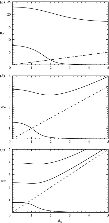
The neutral curves
 ${\it\alpha}_{N}={\it\alpha}_{N}({\it\beta}_{N})$
for (a)
 $y_{N}=0.2$
, (b)
 $y_{N}=1$
and (c)
 $y_{N}=2$
.

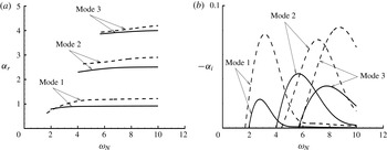
Normalized wavenumber
 ${\it\alpha}_{r}$
(a) and normalized spatial growth rate
 $-{\it\alpha}_{i}$
(b) versus
 ${\it\omega}_{N}$
calculated for
 $y_{N}=2$
. Mode 1: solid line for
 ${\it\beta}_{N}=0.5$
and dashed line for
 ${\it\beta}_{N}=1$
. Modes 2 and 3: solid lines for
 ${\it\beta}=1$
and dashed lines for
 ${\it\beta}_{N}=2$
.

We computed neutral modes for several values of
 $y_{N}$
. As is shown in figure 3, the presence of a shock allows for a countable set of neutral modes. We denote the mode with the smallest
 ${\it\alpha}_{N}$
for a given
 ${\it\beta}_{N}$
as mode 1, and modes 2, 3 and etc. have increasingly larger
 ${\it\alpha}_{N}$
. The bandwidth of these shock-induced instability modes appears to be inversely proportional to
 $y_{N}$
. Their existence is restricted in the region
 ${\it\beta}_{N}<{\it\alpha}_{N}$
except mode-1 family, which continues to the region
 ${\it\beta}_{N}>{\it\alpha}_{N}$
. Modes in this region approach, in the limit
 $y_{N}\rightarrow \infty$
, the more familiar T–S modes whose eigenfunctions attenuate in the upper deck (Smith Reference Smith1989).
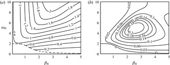
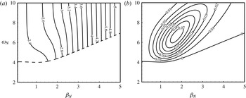
Cowley & Hall (Reference Cowley and Hall1990) calculated only temporal growth rates. Here, we perform a spatial stability analysis, which is considered to be more relevant. Figure 4 displays the wavenumbers and spatial amplification rates of modes 1, 2 and 3. For a fixed
 ${\it\beta}_{N}$
, as
 ${\it\omega}_{N}$
is increased from the neutral frequency, the wavenumber increases; the growth rate increases first, reaches a peak and then decreases, but always remains positive. This is in contrast with the temporal growth rate, which changes its sign repeatedly as the wavenumber increases (Cowley & Hall Reference Cowley and Hall1990).
Contours of wavenumbers (a) and spatial amplification rates (b) of growing modes 1 for the case of
 $y_{N}=2$
. The dashed line in (a) marks the neutral curve, and the decaying modes below it are not considered.

Contours of wavenumbers (a) and spatial amplification rates (b) of growing modes 2 for the case of
 $y_{N}=2$
. The dashed line in (a) marks the neutral curve, and the decaying modes below it are not considered.

In order to provide further information about the instability, we compute the growth rate
 $(-{\it\alpha}_{i})$
and the associated wavenumber for modes 1 and 2 in a fairly large range of
 ${\it\omega}_{N}$
and
 ${\it\beta}_{N}$
. Figures 5 and 6 show the contours of
 $-{\it\alpha}_{i}({\it\omega}_{N},{\it\beta}_{N})$
and
 ${\it\alpha}_{r}({\it\omega}_{N},{\it\beta}_{N})$
on the
 $({\it\omega}_{N},{\it\beta}_{N})$
plane. Overall, the second (and higher) modes have smaller growth rates than those in mode-1 family. For each
 ${\it\omega}_{N}$
, the most unstable mode is oblique. The shock-induced neutral modes form the lower branch of the neutral curve, the unstable region above which appears to extend to infinity suggesting that an upper branch is absent in the triple-deck scaling regime. The results imply that once a lower-branch mode is excited, it will amplify since for a mode with a fixed physical frequency and spanwise wavelength, its non-dimensional frequency and spanwise wavenumber increase as the boundary layer becomes thicker.
The second-order terms in the perturbation expansion (4.25) are governed by equations
 $$\begin{eqnarray}\displaystyle & \displaystyle \text{i}\hat{{\it\alpha}}_{TS}\tilde{U} _{2}+\tilde{V}_{2,Y}+\text{i}\hat{{\it\beta}}_{TS}\tilde{W}_{2}=-A^{\prime }(x_{1})\tilde{U} _{1}, & \displaystyle\end{eqnarray}$$
 $$\begin{eqnarray}\displaystyle & \displaystyle \text{i}(\hat{{\it\alpha}}_{TS}{\it\lambda}_{0}Y-\hat{{\it\omega}}_{TS})\tilde{U} _{2}+{\it\lambda}_{0}\tilde{V}_{2}=\tilde{U} _{2,YY}-{\it\Lambda}(x_{1})Y\tilde{U} _{1}-{\it\lambda}_{1}x_{1}A(x_{1})\tilde{V}_{1}, & \displaystyle\end{eqnarray}$$
 $$\begin{eqnarray}\displaystyle & \displaystyle \text{i}(\hat{{\it\alpha}}_{TS}{\it\lambda}_{0}Y-\hat{{\it\omega}}_{TS})\tilde{W}_{2}=-\text{i}\hat{{\it\beta}}_{TS}\tilde{P}_{2}+\tilde{W}_{2,YY}-{\it\Lambda}(x_{1})Y\tilde{W}_{1}, & \displaystyle\end{eqnarray}$$
 ${\it\Lambda}$
is defined by
 $$\begin{eqnarray}\displaystyle {\it\Lambda}={\it\lambda}_{0}A^{\prime }(x_{1})+\text{i}\hat{{\it\alpha}}_{TS}{\it\lambda}_{1}x_{1}A(x_{1}). & & \displaystyle\end{eqnarray}$$
The no-slip condition on the wall and matching with the main-deck solution imply that
 $\tilde{U} _{2}=\tilde{V}_{2}=\tilde{W}_{2}=0$
at
 $Y=0$
and
 $(\tilde{U} _{2},\tilde{W}_{2})\rightarrow ({\it\lambda}_{0}B_{2}+{\it\lambda}_{1}x_{1}AB_{1},0)$
as
 $Y\rightarrow \infty$
, or equivalently,
 $$\begin{eqnarray}\displaystyle \tilde{V}_{2,YYY}(0)=\hat{{\it\beta}}_{TS}^{2}\tilde{P}_{2};\quad \tilde{V}_{2,Y}\rightarrow -\text{i}\hat{{\it\alpha}}_{TS}{\it\lambda}_{0}B_{2}-{\it\Lambda}(x_{1})B_{1}\quad \text{as }Y\rightarrow \infty . & & \displaystyle\end{eqnarray}$$
Eliminating the pressure
 $\tilde{P}_{2}$
from (4.35) yields
 $$\begin{eqnarray}\displaystyle \left\{\frac{\partial ^{2}}{\partial Y^{2}}-\text{i}(\hat{{\it\alpha}}_{TS}{\it\lambda}_{0}Y-\hat{{\it\omega}}_{TS})\right\}\tilde{V}_{2,YY}={\it\Lambda}(x_{1})Y\tilde{V}_{1,YY}={\it\Lambda}(x_{1})({\it\eta}-{\it\eta}_{0})\,\text{Ai}({\it\eta}), & & \displaystyle\end{eqnarray}$$
which has the solution (cf. Wu Reference Wu1999)
 $$\begin{eqnarray}\displaystyle \tilde{V}_{2,Y}=\frac{1}{3}(\text{i}\hat{{\it\alpha}}_{TS}{\it\lambda}_{0})^{-1}{\it\Lambda}(x_{1})[({\it\eta}-3{\it\eta}_{0})\,\text{Ai}({\it\eta})+2{\it\eta}_{0}\,\text{Ai}({\it\eta}_{0})]+q_{2}\int _{{\it\eta}_{0}}^{{\it\eta}}\,\text{Ai}({\it\eta})\,\text{d}{\it\eta}, & & \displaystyle\end{eqnarray}$$
where
 $q_{2}$
is an unknown function of
 $x_{1}$
. The boundary conditions (4.37) lead to
 $$\begin{eqnarray}\displaystyle & \displaystyle {\textstyle \frac{2}{3}}(\text{i}\hat{{\it\alpha}}_{TS}{\it\lambda}_{0})^{-1/3}{\it\Lambda}[\text{Ai}^{\prime }({\it\eta}_{0})-{\it\eta}_{0}\,\text{Ai}^{\prime \prime }({\it\eta}_{0})]+(\text{i}\hat{{\it\alpha}}_{TS}{\it\lambda}_{0})^{2/3}q_{2}\,\text{Ai}^{\prime }({\it\eta}_{0})=\hat{{\it\beta}}_{TS}^{2}\tilde{P}_{2}, & \displaystyle\end{eqnarray}$$
 $$\begin{eqnarray}\displaystyle & \displaystyle \frac{2}{3}(\text{i}\hat{{\it\alpha}}_{TS}{\it\lambda}_{0})^{-1}{\it\Lambda}{\it\eta}_{0}\,\text{Ai}({\it\eta}_{0})+q_{2}\int _{{\it\eta}_{0}}^{\infty }\,\text{Ai}({\it\eta})\,\text{d}{\it\eta}=-\text{i}\hat{{\it\alpha}}_{TS}{\it\lambda}_{0}B_{2}-{\it\Lambda}B_{1}. & \displaystyle\end{eqnarray}$$
Since the pressure does not change across the main and lower decks, we have
 $$\begin{eqnarray}\displaystyle H_{1}+H_{2}-\frac{\hat{{\it\alpha}}_{TS}}{\hat{{\it\gamma}}_{TS}}\bar{a}_{I}A^{\prime }(1+\text{e}^{2\text{i}\hat{{\it\gamma}}_{TS}\bar{y}_{s}})\bar{y}_{s}=\tilde{P}_{2}. & & \displaystyle\end{eqnarray}$$
Eliminating
 $B_{2}$
and
 $\tilde{P}_{2}$
from (4.18), (4.24), (4.40)–(4.42) and making use of (4.30)–(4.31), we finally obtain the amplitude equation for
 $A$
,
 $$\begin{eqnarray}\displaystyle A^{\prime }(x_{1})={\it\varsigma}x_{1}A+N, & & \displaystyle\end{eqnarray}$$
where
 $$\begin{eqnarray}\displaystyle {\it\varsigma}=-\text{i}\hat{{\it\alpha}}_{TS}{\it\lambda}_{1}b/({\it\lambda}_{0}a),\quad N=-{\it\lambda}_{0}\hat{{\it\gamma}}_{TS}\sec (\hat{{\it\gamma}}_{TS}\bar{y}_{s})J_{0}/a, & & \displaystyle\end{eqnarray}$$
with constants
 $b$
being given by (3.25), and
 $$\begin{eqnarray}\displaystyle a & = & \displaystyle \frac{2}{3}\tan (\hat{{\it\gamma}}_{TS}\bar{y}_{s}){\it\eta}_{0}\,\text{Ai}({\it\eta}_{0})+\left[\frac{\hat{{\it\alpha}}_{TS}^{2}\bar{y}_{s}}{\hat{{\it\gamma}}_{TS}\cos ^{2}(\hat{{\it\gamma}}_{TS}\bar{y}_{s})}-\frac{\hat{{\it\beta}}_{TS}^{2}}{\hat{{\it\gamma}}_{TS}^{2}}\tan (\hat{{\it\gamma}}_{TS}\bar{y}_{s})\right]\int _{{\it\eta}_{0}}^{\infty }\,\text{Ai}({\it\eta})\,\text{d}{\it\eta}\nonumber\\ \displaystyle & & \displaystyle +\,\frac{2\hat{{\it\gamma}}_{TS}(\text{i}\hat{{\it\alpha}}_{TS}{\it\lambda}_{0})^{5/3}}{3\hat{{\it\alpha}}_{TS}^{2}\hat{{\it\beta}}_{TS}^{2}}[\text{Ai}^{\prime }({\it\eta}_{0})-{\it\eta}_{0}^{2}\,\text{Ai}({\it\eta}_{0})].\end{eqnarray}$$
5 Matching and coupling coefficients
5.1 Matching with the pre-resonance region
On assuming that the amplitude of the T–S wave vanishes as
 $x_{1}\rightarrow -\infty$
, the amplitude equation (4.43) has the solution
 $$\begin{eqnarray}\displaystyle A(x_{1})=N\text{e}^{{\it\varsigma}{x_{1}}^{2}/2}\int _{-\infty }^{x_{1}}\text{e}^{-{\it\varsigma}{\it\xi}^{2}/2}\,\text{d}{\it\xi}. & & \displaystyle\end{eqnarray}$$
More precisely, it can be shown that
 $$\begin{eqnarray}\displaystyle A(x_{1})\rightarrow (N/{\it\varsigma})(-x_{1})^{-1}+O(x_{1}^{-3})\quad \text{as }x_{1}\rightarrow -\infty . & & \displaystyle\end{eqnarray}$$
The above behaviour implies matching with the upstream response. To illustrate this, we take the pressure
 $p$
as an example. In the upper deck, the pressure
 $p$
is given by
 $$\begin{eqnarray}\displaystyle p={\it\delta}Re^{3/16}{\it\mu}_{w}^{-3/16}T_{w}^{-9/16}M^{-3/8}A(x_{1})[\bar{a}_{I}\text{e}^{\text{i}\hat{{\it\gamma}}_{TS}\bar{y}}+\bar{a}_{R}\text{e}^{-\text{i}\hat{{\it\gamma}}_{TS}\bar{y}}]\tilde{E}+\text{c.c.}, & & \displaystyle\end{eqnarray}$$
where
 $\bar{a}_{I}$
and
 $\bar{a}_{R}$
are found from (4.30)–(4.31) as
 $$\begin{eqnarray}\displaystyle \bar{a}_{I,R}=\mp \frac{\hat{{\it\alpha}}_{TS}\text{e}^{\mp \text{i}\hat{{\it\gamma}}_{TS}\bar{y}_{s}}}{2{\it\lambda}_{0}\hat{{\it\gamma}}_{TS}\cos (\hat{{\it\gamma}}_{TS}\bar{y}_{s})}\int _{{\it\eta}_{0}}^{\infty }\,\text{Ai}({\it\eta})\,\text{d}{\it\eta}. & & \displaystyle\end{eqnarray}$$
Using (5.2), (4.44) and (2.45), we find that
 $$\begin{eqnarray}\displaystyle \bar{a}_{I,R}A(x_{1})\rightarrow \left\{\frac{x_{0}J_{0}[\tan (\hat{{\it\gamma}}_{TS}\bar{y}_{s})\pm \text{i}]}{b\cos (\hat{{\it\gamma}}_{TS}\bar{y}_{s})}\int _{{\it\eta}_{0}}^{\infty }\,\text{Ai}({\it\eta})\,\text{d}{\it\eta}\right\}x_{1}^{-1}\quad \text{as }x_{1}\rightarrow -\infty . & & \displaystyle\end{eqnarray}$$
Comparison with (3.24) shows that
 $$\begin{eqnarray}\displaystyle Re^{3/16}{\it\mu}_{w}^{-3/16}T_{w}^{-9/16}M^{-3/8}A(x_{1})\bar{a}_{I,R}\rightarrow a_{I,R}\quad \text{as }x_{1}\rightarrow -\infty , & & \displaystyle\end{eqnarray}$$
which is precisely what is required for the matching of the pressure in the two stages.
5.2 Coupling coefficients
We now turn to the downstream limit,
 $x_{1}\rightarrow +\infty$
. In this limit,
 $$\begin{eqnarray}\displaystyle A(x_{1})\rightarrow A_{\infty }\text{e}^{{\it\varsigma}{x_{1}}^{2}/2},\quad \text{with }A_{\infty }=N\int _{-\infty }^{\infty }\text{e}^{-{\it\varsigma}{\it\xi}^{2}/2}\,\text{d}{\it\xi}=N\sqrt{2{\rm\pi}/{\it\varsigma}}. & & \displaystyle\end{eqnarray}$$
In the post-resonance stage corresponding to
 $x_{1}=O(\bar{{\it\epsilon}}^{-1})$
, the amplitude of the excited T–S mode,
 $A\text{e}^{\text{i}\hat{{\it\alpha}}_{TS}\bar{x}}$
, is replaced by the usual WKBJ form
 $$\begin{eqnarray}\displaystyle A_{\infty }\exp \left\{\text{i}Re^{3/8}{\it\mu}_{w}^{-3/8}T_{w}^{-9/8}M^{-3/4}\int _{x_{0}}^{x}\hat{{\it\alpha}}_{TS}(x)\,\text{d}x\right\}, & & \displaystyle\end{eqnarray}$$
where the complex wavenumber
 $\hat{{\it\alpha}}_{TS}(x)$
is determined by the local parallel stability theory. Clearly, the constant
 $A_{\infty }$
appears as the (scaled) initial amplitude.
In order to be precise, we use the maximum value of the streamwise velocity of the T–S wave as an indicator of its magnitude. First, inserting
 $\tilde{P}_{1}$
found from (4.30) into the spanwise momentum equation in (4.26), we may express the spanwise velocity as
 $\tilde{W}_{1}=(\text{i}\,\text{Ai}^{\prime }({\it\eta}_{0})/\hat{{\it\beta}}_{TS})L({\it\eta})$
, where
 $L({\it\eta})$
is the solution to the boundary-value problem:
 $$\begin{eqnarray}\displaystyle L^{\prime \prime }-{\it\eta}L=1,\quad L({\it\eta}_{0})=0;\quad L\rightarrow 0\quad \text{as }{\it\eta}\rightarrow \infty . & & \displaystyle\end{eqnarray}$$
From the continuity equation, the streamwise velocity is obtained and its maximum magnitude at the neutral point is given by (cf. Wu Reference Wu1999)
 $$\begin{eqnarray}\displaystyle u_{TS}={\it\delta}Re^{5/16}{\it\mu}_{w}^{-5/16}T_{w}^{1/16}M^{11/8}\hat{{\it\alpha}}_{TS}^{-1}A_{\infty }U_{m}, & & \displaystyle\end{eqnarray}$$
where
 $$\begin{eqnarray}\displaystyle U_{m}=\max _{{\it\eta}}\left|\int _{{\it\eta}_{0}}^{{\it\eta}}\,\text{Ai}({\it\eta})\,\text{d}{\it\eta}-\text{Ai}^{\prime }({\it\eta}_{0})L({\it\eta})\right|. & & \displaystyle\end{eqnarray}$$
Following the practice in experiments, we normalize the dimensional frequency of the disturbance
 $\breve{{\it\omega}}$
as
 $$\begin{eqnarray}\displaystyle f=\breve{{\it\omega}}\breve{{\it\nu}}_{s}/\breve{U}_{s}^{2}, & & \displaystyle\end{eqnarray}$$
For the rescalings (2.33), we find by using (4.33)–(4.34) that the neutral position, non-dimensionalized by
 $\breve{{\it\mu}}_{s}/\breve{{\it\rho}}_{s}\breve{U}_{s}$
, is given by
 $$\begin{eqnarray}\displaystyle \tilde{x}_{0}\equiv \frac{\breve{{\it\rho}}_{s}\breve{U}_{s}\breve{x}_{0}}{\breve{{\it\mu}}_{s}}={\it\mu}_{w}^{-1/3}T_{w}^{-1}M^{-2/3}{\it\lambda}_{0}^{2}(f/{\it\omega}_{N})^{-4/3}. & & \displaystyle\end{eqnarray}$$
The streamwise length scale
 $\breve{l}$
can be taken as
 $\breve{x}_{0}$
so that
 $x_{0}=1$
,
 ${\it\lambda}_{0}={\it\chi}$
and the Reynolds number
 $Re$
is actually
 $\tilde{x}_{0}$
.
We define the coupling coefficient for the fast/slow acoustic waves respectively as
 $$\begin{eqnarray}\displaystyle C_{A}^{\pm }=u_{TS}/{\it\delta}p_{I}^{\pm }, & & \displaystyle\end{eqnarray}$$
and it follows from (5.7), (4.44) and (5.12)–(5.13) that
 $$\begin{eqnarray}\displaystyle C_{A}^{\pm }=\frac{2}{2-\bar{{\it\gamma}}}{\it\sigma}^{2}{\it\mu}_{w}^{-5/12}T_{w}^{-1/4}M^{19/6}f^{-5/12}{\it\kappa}, & & \displaystyle\end{eqnarray}$$
where
 $$\begin{eqnarray}\displaystyle {\it\kappa}({\it\beta}_{N},y_{N})=\sqrt{2{\rm\pi}}{\it\chi}^{13/8}{\it\omega}_{N}^{5/12}\sqrt{1-({\it\beta}_{N}/{\it\alpha}_{N})^{2}}\sec \left(\sqrt{{\it\alpha}_{N}^{2}-{\it\beta}_{N}^{2}}y_{N}\right)U_{m}/|a\sqrt{{\it\varsigma}}|.\qquad & & \displaystyle\end{eqnarray}$$
Similarly, we define the coupling coefficients for the vorticity and entropy waves respectively as
 $$\begin{eqnarray}\displaystyle C_{V}\equiv u_{TS}/{\it\delta}v_{I},\quad C_{E}\equiv u_{TS}/{\it\delta}r_{I}. & & \displaystyle\end{eqnarray}$$
It is found that
 $C_{V}$
and
 $C_{E}$
scale with
 $f$
and
 $M$
as
 $$\begin{eqnarray}\displaystyle C_{V}=2{\it\sigma}^{-1}{\it\mu}_{w}^{-5/12}T_{w}^{-1/4}M^{-5/6}f^{-5/12}{\it\kappa},\quad C_{E}={\it\sigma}^{2}{\it\mu}_{w}^{-5/12}T_{w}^{-1/4}M^{7/6}f^{-5/12}{\it\kappa}.\qquad & & \displaystyle\end{eqnarray}$$
6 Numerical results
6.1 Boundary-layer response in the pre-resonance region
The boundary-layer responds to a broadband of free-stream disturbances, including to vortical and entropy disturbances since they generate acoustic waves downstream of the shock. We first consider the characteristics of the response at a fixed streamwise location
 $x$
. The dependence on
 $x$
is through
 ${\it\lambda}$
with
 $x$
acting as a parameter, and it can be scaled out by setting
 $$\begin{eqnarray}\displaystyle \hat{{\it\alpha}}_{a}={\it\lambda}^{5/4}{\it\alpha}_{A},\quad \hat{{\it\beta}}_{a}={\it\lambda}^{5/4}{\it\beta}_{A},\quad \hat{{\it\omega}}_{a}={\it\lambda}^{3/2}{\it\omega}_{A},\quad \bar{y}_{s}={\it\lambda}^{-5/4}y_{A}. & & \displaystyle\end{eqnarray}$$
Contours of
 $|a_{I}/J_{0}|$
and
 $|\mathscr{R}|$
in the
 ${\it\alpha}_{A}{-}{\it\omega}_{A}$
plane for
 $y_{A}=1$
and
 ${\it\beta}_{A}=0.5$
. The dashed lines in (a) represent the loci of (6.4) for
 $n=1,2$
.

As an illustration, calculations are performed for
 $y_{A}=1$
and
 ${\it\beta}_{A}=0.5$
with
 ${\it\alpha}_{A}$
and
 ${\it\omega}_{A}$
in the range
 $1\leqslant {\it\alpha}_{A}\leqslant 6$
and
 $0<{\it\omega}_{A}\leqslant 10$
. Figure 7 shows the contours of
 $|a_{I}/J_{0}|$
and
 $|\mathscr{R}|$
; contours of
 $|a_{R}/J_{0}|$
look similar to those of
 $|a_{I}/J_{0}|$
and hence are not shown. The response is finite for all
 $({\it\alpha}_{A},{\it\omega}_{A})$
except when
 $({\it\alpha}_{A},{\it\omega}_{A})=(1.46,2.95)$
and
 $(4.65,6.40)$
, which correspond to neutral modes 1 and 2 respectively. A striking feature is that there is an extremely strong response to a broadband of high-frequency free-stream disturbances within a narrow band of
 ${\it\alpha}_{A}$
, represented by the two narrow and almost vertical strips in the figure. In order to explain this, an analysis of (3.21) is performed in the high-frequency limit
 $\hat{{\it\omega}}_{a}\gg 1$
. For a general
 ${\it\alpha}_{A}$
, both the numerator and the denominator
 ${\it\Delta}$
are of
 $O(1)$
. However, the latter reduces to
 $O({\it\omega}_{A}^{-5/2})$
if
 ${\it\alpha}_{A}$
is sufficiently close to
 $$\begin{eqnarray}\displaystyle {\it\alpha}_{c}=\left[\left[\frac{(2n-1){\rm\pi}}{2y_{A}}\right]^{2}+{\it\beta}_{A}^{2}\right]^{1/2}\quad (n=1,2,\ldots ), & & \displaystyle\end{eqnarray}$$
while the numerator remains of
 $O(1)$
so that
 $a_{I,R}/J_{0}$
raises to
 $O({\it\omega}_{A}^{5/2})$
. More precisely, the analysis shows that
 $$\begin{eqnarray}\displaystyle a_{I,R}/J_{0}\sim (-1)^{n}\frac{(2n-1){\rm\pi}\text{e}^{-{\rm\pi}\text{i}/4}}{4{\it\alpha}_{c}^{2}{\it\beta}_{A}^{2}y_{A}}{\it\omega}_{A}^{5/2}, & & \displaystyle\end{eqnarray}$$
when
 $$\begin{eqnarray}\displaystyle {\it\alpha}_{A}={\it\alpha}_{c}-({\it\beta}_{A}^{2}/y_{A}){\it\omega}_{A}^{-1}-\frac{2{\it\beta}_{A}^{6}}{(2n-1)^{2}{\rm\pi}^{2}{\it\alpha}_{c}}{\it\omega}_{A}^{-2}\quad \text{and}\quad {\it\omega}_{A}\gg 1. & & \displaystyle\end{eqnarray}$$
The loci of (6.4) are marked by the dashed lines in figure 7(a). Figure 8 compares the numerical result with the asymptotic approximation (6.3). A good agreement is observed. The strong response is therefore due to the fact that the dispersion function
 ${\it\Delta}$
almost vanishes for
 ${\it\alpha}_{A}$
and
 ${\it\omega}_{A}$
specified by (6.4), and we will refer to this as quasi- or near resonance (which differs from the exact resonance corresponding to
 ${\it\Delta}=0$
). The quasi-resonance is of broadband nature with respect to the frequency but highly selective with respect to the wavenumber. For each
 ${\it\beta}_{A}$
, there exists a series of strips centred at the curves as specified by (6.4). In the presence of a broadband of free-stream disturbances, the boundary layer acts as a high-pass amplifier. Figure 7(b) indicates that for relatively low frequencies
 $|\mathscr{R}|<1$
, that is, the boundary layer absorbs some of the incident acoustic wave energy. In contrast, for high-frequency waves,
 $|\mathscr{R}|>1$
, implying that the wave reflected by the viscous boundary layer is stronger than the incident wave, a phenomenon referred to as over-reflection.


Variation of
 $|a_{I}/J_{0}|$
and
 $|\mathscr{R}|$
with
 ${\it\omega}_{A}$
for
 ${\it\alpha}_{A}$
being the wavenumber of mode 1.

We are primarily interested in cases where an exact resonance with a T–S wave can take place, and thus in subsequent calculations for each
 ${\it\beta}_{A}$
the rescaled wavenumber
 ${\it\alpha}_{A}$
is taken to be that determined by the first relation in (4.34) for modes 1 and 2. The computed
 $|a_{I}/J_{0}|$
and
 $|\mathscr{R}|$
as functions of
 ${\it\omega}_{A}$
are shown in figure 9 for mode 1;
 $|a_{R}/J_{0}|$
is not shown as it resembles
 $|a_{I}/J_{0}|$
. The response is finite for
 ${\it\omega}_{A}\neq {\it\omega}_{N}$
, but becomes infinite as the frequency approaches the local neutral frequency
 ${\it\omega}_{N}$
of mode 1, indicating an exact resonance between the sound wave and the neutral T–S mode. Figure 9(a) shows that
 $|a_{I}/J_{0}|$
is larger for smaller spanwise wavenumbers. Figure 9(b) indicates
 $|\mathscr{R}|<1$
for low frequencies and
 $|\mathscr{R}|>1$
for high frequencies as observed earlier. Interestingly, (3.23) indicates that
 $$\begin{eqnarray}\displaystyle \mathscr{R}\rightarrow \frac{\tan (\hat{{\it\gamma}}_{a}\bar{y}_{s})-\text{i}}{\tan (\hat{{\it\gamma}}_{a}\bar{y}_{s})+\text{i}}\quad \text{as }{\it\omega}_{A}\rightarrow {\it\omega}_{N}, & & \displaystyle\end{eqnarray}$$
so that
 $|\mathscr{R}|\rightarrow 1$
. The parameter region of over-reflection,
 ${\it\omega}_{A}>{\it\omega}_{N}$
, corresponds to the unstable regime above the neutral curve. The present consideration of reflection thus provides a physical interpretation of the shock-induced instability. A similar instability arises in the supersonic twin boundary layers developing along two parallel plates (Wu Reference Wu2014).
Variation of
 $|a_{I}/J_{0}|$
and
 $|\mathscr{R}|$
with
 ${\it\omega}_{A}$
for
 ${\it\alpha}_{A}$
being the wavenumber of mode 2.

Figure 10(a,b) depicts the variations of
 $|a_{I}/J_{0}|$
and
 $|\mathscr{R}|$
with the frequency
 ${\it\omega}_{A}$
for different spanwise wavenumbers
 ${\it\beta}_{A}$
with
 ${\it\alpha}_{A}$
being the wavenumber of mode 2. The amplitudes
 $|a_{I}/J_{0}|$
and
 $|a_{R}/J_{0}|$
(not shown) first decrease and then increase as the spanwise wavenumber
 ${\it\beta}_{A}$
varies from
 $0.5$
to
 $5.0$
in both the low- and high-frequency regions. This may be associated with the non-monotonicity of the neutral curve of mode 2 (see figure 3). The reflection coefficient
 $|\mathscr{R}|$
exhibits a similar feature to that in figure 9(b):
 $|\mathscr{R}|<1$
for low-frequency waves and
 $|\mathscr{R}|>1$
for high-frequency waves with
 $|\mathscr{R}|=1$
on the neutral curve, signalling that the onset of the instability corresponds to over-reflection.
Next, we consider the response at different streamwise locations for fixed physical frequencies
 $\hat{{\it\omega}}_{a}$
and wavenumbers
 $\hat{{\it\alpha}}_{a}$
and
 $\hat{{\it\beta}}_{a}$
. The latter two are specified as
 $$\begin{eqnarray}\displaystyle \hat{{\it\alpha}}_{a}={\it\chi}^{5/4}{\it\alpha}_{N},\quad \hat{{\it\beta}}_{a}={\it\chi}^{5/4}{\it\beta}_{N}, & & \displaystyle\end{eqnarray}$$
where
 ${\it\chi}=0.332$
, and
 ${\it\alpha}_{N}$
and
 ${\it\beta}_{N}$
are on the neutral curves of mode 1 or 2. The calculations were performed for
 $\bar{y}_{s}={\it\chi}^{-5/4}x$
with
 $0<x\leqslant 1.2$
. For the case of
 ${\it\beta}_{N}=0.5$
and
 ${\it\alpha}_{N}$
being on the neutral curve of mode 1, contours of
 $|a_{I}/J_{0}|$
are displayed in figure 11. A broadband of strong high-frequency disturbances appears at almost the same streamwise location, owing again to the quasi-resonance. A high-frequency analysis of (3.21) for fixed
 ${\it\alpha}_{N}$
and
 ${\it\beta}_{N}$
shows that the response raises to
 $O((\hat{{\it\omega}}_{a}/{\it\chi}^{3/2})^{5/2})$
, or more precisely,
 $$\begin{eqnarray}\displaystyle a_{I,R}/J_{0}\sim (-1)^{n}\frac{({\it\alpha}_{N}^{2}-{\it\beta}_{N}^{2})^{1/2}\text{e}^{-{\rm\pi}\text{i}/4}}{2{\it\alpha}_{N}^{2}{\it\beta}_{N}^{2}{\it\chi}^{15/4}}\hat{{\it\omega}}_{a}^{5/2}, & & \displaystyle\end{eqnarray}$$
when
 $$\begin{eqnarray}\displaystyle x=x_{c}-\frac{{\it\alpha}_{N}{\it\beta}_{N}^{2}x_{c}^{1/2}{\it\chi}^{3/2}}{{\it\alpha}_{N}^{2}-{\it\beta}_{N}^{2}}\hat{{\it\omega}}_{a}^{-1}-\frac{{\it\alpha}_{N}^{2}{\it\beta}_{N}^{4}{\it\chi}^{3}}{2({\it\alpha}_{N}^{2}-{\it\beta}_{N}^{2})^{2}}\hat{{\it\omega}}_{a}^{-2}\quad \text{and}\quad \hat{{\it\omega}}_{a}\gg 1, & & \displaystyle\end{eqnarray}$$
where
 $$\begin{eqnarray}\displaystyle x_{c}=\frac{(2n-1){\rm\pi}}{2({\it\alpha}_{N}^{2}-{\it\beta}_{N}^{2})^{1/2}}\quad (n=1,2,\ldots ). & & \displaystyle\end{eqnarray}$$
The locus of (6.8), in the vicinity of which the response is the strongest, is indicated by the dashed line in figure 11.
Contours of
 $|a_{I}/J_{0}|$
and
 $|\mathscr{R}|$
in the
 $x{-}\hat{{\it\omega}}_{a}/{\it\chi}^{3/2}$
plane for
 $\bar{y}_{s}={\it\chi}^{-5/4}x$
and
 ${\it\beta}_{N}=0.5$
. The dashed line represents the locus of (6.8).

Exact resonance occurs (at
 $x=x_{0}=1$
) when
 $\hat{{\it\omega}}_{a}={\it\chi}^{3/2}{\it\omega}_{N}$
. Figure 12 shows
 $|a_{I}/J_{0}|$
and
 $|\mathscr{R}|$
as functions of
 $x$
when the frequency is that of mode 1. The variation pattern of
 $|a_{I}/J_{0}|$
and
 $|\mathscr{R}|$
is similar to that displayed in figures 9 and 10. The response is finite upstream of the neutral position
 $x_{0}=1$
, but becomes infinite as
 $x\rightarrow x_{0}$
. The response is stronger for disturbances with larger spanwise wavenumbers. Figure 12(b) indicates that
 $|\mathscr{R}|<1$
for
 $x<x_{0}=1$
, and
 $|\mathscr{R}|\rightarrow 1$
when
 $x$
approaches the neutral point, downstream of which
 $|\mathscr{R}|>1$
(not shown), i.e. over-reflection takes place in the unstable region. Figure 13(a,b) displays the variation of
 $|a_{I}/J_{0}|$
and
 $|\mathscr{R}|$
with
 $x$
for different spanwise wavenumbers and the frequency being that of mode 2. Again, the amplitude of the response first decreases with the spanwise wavenumber and then increases, possibly due to the non-monotonicity of the neutral curve of mode 2. The reflection coefficient
 $|\mathscr{R}|$
(figure 13
b) exhibits a similar feature to that of mode 1.
Variation of
 $|a_{I}/J_{0}|$
and
 $|\mathscr{R}|$
with
 $x$
for
 ${\it\alpha}_{N}$
being the wavenumber of mode 1.

Variation of
 $|a_{I}/J_{0}|$
and
 $|\mathscr{R}|$
with
 $x$
for
 ${\it\alpha}_{N}$
being the wavenumber of mode 2.

The response of a supersonic boundary layer to incident slow acoustic waves was studied previously by Gaponov (Reference Gaponov1977), who used the linearized N–S equations but neglected the streamwise and spanwise diffusion as well as the effect of a shock. Over-reflection was observed, but an exact resonance with an eigenmode does not occur. Both phenomena may take place when acoustic waves interact with a supersonic vortex sheet (Ribner Reference Ribner1957), where the eigenmodes are a compressible version of Kelvin–Helmholtz instability waves.
Variation of
 ${\it\kappa}$
with
 ${\it\beta}_{N}$
for (a)
 $y_{N}=0.2$
, (b)
 $y_{N}=1$
and (c)
 $y_{N}=2$
. ——, mode 1; – ⋅ – ⋅ –, mode 2; – – –, mode 3. The curves —▿— in (a) and (b) represent
 ${\it\kappa}/200$
and
 ${\it\kappa}/20$
respectively.

6.2 Results for coupling coefficients
In order to gain quantitative information about the efficiency of the receptivity, the dependence of
 ${\it\kappa}$
on the parameters is investigated. Figure 14 shows
 ${\it\kappa}$
for modes 1, 2 and 3, and for different shock locations. The mode-1 family stands out: the coupling coefficient is significantly larger than those for modes 2 and 3, and especially for modes in the region
 ${\it\beta}_{N}>{\it\alpha}_{N}$
, where
 ${\it\kappa}$
is approximately 100 and 10 times larger for
 $y_{N}=0.2$
and
 $1$
, respectively. It may be worth noting that when
 ${\it\beta}_{N}>{\it\alpha}_{N}$
, the induced acoustic perturbation downstream of the shock is not purely sinusoidal in the direction normal to the shock. Rather it consists of two components, among which one amplifies while the other attenuates exponentially. Despite this difference, the perturbation exhibits, in terms of its phase speed, the key characteristics of a slow acoustic wave. For small
 ${\it\beta}_{N}$
, the value of
 ${\it\kappa}$
for mode 2 is larger than that for mode 3, but there is a cross-over when
 ${\it\beta}_{N}$
exceeds a critical value. As the shock position
 $y_{N}$
increases, the value of
 ${\it\kappa}$
decreases for all three modes, implying that the coupling is weaker when the shock becomes more distant to the wall.
Variation of coupling coefficients
 $C_{A}^{\pm }$
,
 $C_{V}$
and
 $C_{E}$
with
 ${\it\beta}_{N}$
for a wedge with a half-angle of 20°,
 $M_{u}=20$
and
 $Re=5.0\times 10^{6}$
, which corresponds to
 $y_{N}\approx 0.2$
.

Figure 14 indicates that
 ${\it\kappa}=O(1)$
for typical
 $O(1)$
values of
 ${\it\beta}_{N}$
and
 $y_{N}$
. However, the factors multiplying
 ${\it\kappa}$
in
 $C_{A}^{\pm }$
,
 $C_{V}$
and
 $C_{E}$
are large and so are these coupling coefficients. A calculation performed for a wedge with a half-angle of
 ${\rm\pi}/9$
(i.e. 20°),
 $M_{u}=20$
(
 $M\approx 14$
) and
 $Re=5.0\times 10^{6}$
(for which
 $y_{N}\approx 0.2$
). The coupling coefficients for mode 1 with
 $0<{\it\beta}_{N}<2$
are shown in figure 15. The result indicates extraordinarily efficiency, which is caused by the resonant nature of the receptivity mechanism. Among three types of free-stream disturbances, acoustic waves are most efficient due to the amplification effect of shock at large-
 $M$
limit as (A 43) indicates. Entropy fluctuations come the second and vortical perturbations are least efficient of the three by comparison. Specifically for
 ${\it\beta}_{N}=1.5$
, it is found that for mode 1 (
 ${\it\omega}_{N}=6.1$
),
 ${\it\kappa}=2.01$
,
 $$\begin{eqnarray}\displaystyle C_{A}^{\pm }=0.144\times 10^{6}\,{\it\kappa},\quad C_{V}=0.846\times 10^{2}\,{\it\kappa},\quad C_{E}=0.360\times 10^{3}\,{\it\kappa}, & & \displaystyle\end{eqnarray}$$
and for mode 2 (
 ${\it\omega}_{N}=17.8$
),
 ${\it\kappa}=0.43$
,
 $$\begin{eqnarray}\displaystyle C_{A}^{\pm }=0.092\times 10^{6}\,{\it\kappa},\quad C_{V}=0.542\times 10^{2}\,{\it\kappa},\quad C_{E}=0.230\times 10^{3}\,{\it\kappa}. & & \displaystyle\end{eqnarray}$$
The absolute initial amplitude of the excited T–S mode depends on the level of fluctuations in the oncoming flow. The presence of a pressure fluctuation
 ${\it\delta}p_{I}=O(10^{-7})$
(which corresponds to a velocity fluctuation of
 $O(M_{u}{\it\delta}p_{I})=O(10^{-6})$
),
 ${\it\delta}v_{I}=O(10^{-4})$
and
 ${\it\delta}r_{I}=O(10^{-4})$
would generate T–S modes with initial amplitudes as large as a few per cent. The turbulence (noise) level in wind tunnels is usually higher than these by one or two orders of magnitude. Perturbations in flight conditions are thought to be weak, e.g. at cruise altitudes of civil aircrafts, the turbulence level, in terms of velocity fluctuations, is thought to be of
 $O(10^{-4})$
with respect to a transonic flight speed. That translates to
 $O(10^{-5})$
velocity fluctuation at
 $M_{u}=20$
. On the other hand, density fluctuations of
 $O(10^{-5})$
(which is independent of the flight speed) are very likely. Vortical or density perturbations of this level are capable of generating T–S waves with initial magnitudes in the range of
 $0.1-1\%$
, which is quite substantial. If velocity fluctuations of
 $O(10^{-5})$
are primarily acoustic, the amplitude of T–S modes excited could be as large as
 $10\%$
, but of course in this case the validity of the present linear theory may be questioned.
Finally, it is worth noting that
 ${\it\kappa}\rightarrow 0$
as
 ${\it\beta}_{N}\rightarrow 0$
. The present mechanism thus operates primarily for three-dimensional disturbances. Two-dimensional ones are probably more likely to excite instability modes through the leading-edge mechanism of Fedorov & Khokhlov (Reference Fedorov and Khokhlov1991) and Fedorov (Reference Fedorov2003). However, if planar modes on the triple-deck scales are to be excited, new mechanisms must be sought.
7 Summary and conclusions
In this paper, the response and receptivity of the boundary layer over a wedge to free-stream disturbances including acoustic, vortical and entropy perturbations were investigated theoretically in the limit of asymptotically large Reynolds and Mach numbers. We consider the case where the angle between the shock and the wedge is small so that the shock lies just at the outer edge of the boundary layer. In this case, there exist instability modes which assume a triple-deck structure and whose eigenfunctions are oscillatory in the upper deck. We focus on free-stream disturbances whose characteristic frequency and wavelength are also on the triple-deck scales. The boundary-layer response is viscous. Any of the three types of perturbations interacts with the shock to generate an acoustic perturbation, and thus free-stream vortical and entropy waves, like acoustic waves, can also drive velocity and temperature fluctuations in the boundary layer. A continuum of high-frequency disturbances within a narrow band of streamwise wavenumber was found to be in quasi-resonance with the eigenmodes thereby generating remarkably strong boundary-layer response. This interesting phenomenon does not appear to have been reported before. We also monitored the behaviour of the reflection coefficient
 $\mathscr{R}$
, defined as the ratio of the amplitude of the outgoing acoustic wave to that of the incoming wave, and noted that
 $|\mathscr{R}|<1$
upstream of the neutral point, and
 $|\mathscr{R}|>1$
downstream. The shock-induced instability can therefore be interpreted as over-reflection of acoustic waves by the boundary layer.
Among broadband three-dimensional free-stream perturbations, there exist components which generate slow acoustic waves whose streamwise and spanwise wavelengths coincide with those of neutral T–S modes. The response to each of these components evolves through three stages, referred to as the pre-resonance, resonance and post-resonance stages. In the pre-resonance stage, the response, consisting of incoming and outgoing slow acoustic waves, is finite. The amplitudes of these two waves become unbounded as the neutral point of the corresponding T–S wave is approached. The disturbance enters the resonance stage in the vicinity of the neutral point, where the slow acoustic wave resonates with the T–S eigenmode. By using the matched asymptotic expansion and multiple scale methods simultaneously, an amplitude equation was derived to describe the evolution of the upstream response into a nearly neutral T–S wave, which becomes an unstable mode in the post-resonance stage further downstream. By matching between different stages, the initial amplitude of the T–S wave and appropriate coupling coefficients are defined. The present mechanism is new and unique in the following sense. On the one hand, unlike the leading-edge mechanisms (Goldstein Reference Goldstein1983; Fedorov & Khokhlov Reference Fedorov and Khokhlov1991; Fedorov Reference Fedorov2003), the conversion into eigenmodes takes place further downstream and locally, in the vicinity of the lower-branch neutral curve. Another difference is that the presence of a shock is crucial for the present mechanism, but it is not for that of Fedorov & Khokhlov (Reference Fedorov and Khokhlov1991). On the other hand, each of acoustic, vortical and entropy perturbations alone may generate a T–S wave without resorting to interaction among themselves (cf. Wu Reference Wu1999) or with a surface roughness element (cf. Ruban Reference Ruban1984; Goldstein Reference Goldstein1985). For these reasons the mechanism is also very efficient. Among three different types of perturbations, fast and slow acoustic waves turn out to be the most efficient, which is also the case in the leading-edge mechanism (Fedorov & Khokhlov Reference Fedorov and Khokhlov2001). The coupling coefficient decreases as the distance of the shock to the wall increases, and is smaller for higher modes. The coupling coefficient vanishes when the oncoming disturbance is two-dimensional, that is, the mechanism operates primarily for three-dimensional disturbances. The practice relevance of the present mechanism and its importance relative to the existing ones depend on a number of factors including the intensity and spectrum of the free-stream disturbances, the Mach number, the location of shock as well as surface roughness. A comparative study in the multi-dimensional parameter space is needed but is beyond the scope of this paper.
DNS investigations by Ma & Zhong (Reference Ma and Zhong2003b
, Reference Ma and Zhong2005) and by Balakumar (Reference Balakumar2003, Reference Balakumar2005) have indicated too that planar acoustic, vortical and entropy disturbances alone can excite instability modes in a supersonic flat-plate boundary layer. These careful numerical studies have provided much important information about supersonic boundary-layer receptivity. The precise mechanisms however remain to be fully understood. The numerical results were primarily interpreted in terms of the leading-edge mechanism of Fedorov & Khokhlov (Reference Fedorov and Khokhlov1991), which is most likely to be operating since the external disturbances are two-dimensional. For three-dimensional disturbances, the present new mechanism may be relevant too, but DNS in three dimensions is necessary in order to shed further light on it. The two mechanisms can be differentiated since they operate, as was emphasized above, in different streamwise regions, and tend to excite modes of distinct characters. The mechanism of Fedorov & Khokhlov (Reference Fedorov and Khokhlov1991) generates modes with
 $O(1)$
phase speeds and with spanwise wavenumbers
 ${\it\beta}<\sqrt{M^{2}-1}\,{\it\alpha}$
. The present mechanism excite modes with phase speeds appreciably smaller than unity, among which high modes have spanwise wavenumbers
 ${\it\beta}>\sqrt{M^{2}-1}\,{\it\alpha}$
, but the first mode is not subject to this restriction provided that
 ${\it\beta}\neq 0$
.
Gaponov (Reference Gaponov, Lin, Phillips and Valentine1993) also considered excitation of instability waves in a supersonic flat-plate boundary layer by slow sound waves. However, without accounting for the presence of a shock, exact resonance with instability modes, which is instrumental in the mechanism described in the present paper, does not occur, that is, if a sound wave and an instability mode have the same frequency, their phase speeds would differ by a finite amount and so do their streamwise wavenumbers. The differences are fairly small numerically nevertheless, and so when a sound wave is refracted by the non-parallel boundary-layer flow, its phase speed/streamwise wavenumber may be tuned to match those of the instability mode so that the forcing resulting from refraction then excites the latter. This is clearly a different physical mechanism from what is described in the present paper, and it is also not as efficient. Mathematically, Gaponov (Reference Gaponov, Lin, Phillips and Valentine1993) used a heuristic non-asymptotic approach to calculate the coupling coefficient. Surprisingly, the strongest excitation was found to occur at the location of zero reflection.
It is known that at high Mach numbers, planar second Mack modes overall have the largest growth rates, but among first Mack modes the most amplified is three-dimensional. The present receptivity excites highly oblique waves, which may be considered as first Mack modes in their earlier stage (i.e. near the lower branch). When such a wave propagates downstream, its physical frequency and spanwise wavelength, remain fixed so that the non-dimensional frequency and spanwise wavenumber, normalized by the local boundary-layer thickness, will increase. The wave continues to amplify according to the result shown in figures 5 and 6. It remains to be seen if some of these oblique modes would evolve into a predominantly inviscid regime and end up as nearly the most amplified modes. The answer to this question requires stability calculations to be performed in an extensive streamwise region well beyond the lower-branch triple-deck regime. On the other hand, in view of strong boundary-layer fluctuations generated through the quasi-resonance and the large amplitude of T–S waves excited through the exact resonance, the response and receptivity may well be nonlinear. Furthermore, the intense perturbations may even cause bypass transition. These issues merit further investigations.
Acknowledgement
The authors would like to thank Professor P. Hall, Professor A. I. Ruban, Dr S. J. Cowley and the referees for helpful comments and suggestions. This work was supported by the NSFC (grants 11172204 and 11332007).
Appendix A. Shock conditions
In this appendix, we consider the conditions which hold at the shock, the position of which is taken to be at
 ${\it\eta}=f({\it\xi},z,t;x_{1})$
. The disturbance upstream is given by (2.13) along with (2.14) and (2.17)–(2.18), while that downstream is expressed by (2.21). In the presence of the small-amplitude disturbance, the shock is slightly perturbed from
 ${\it\eta}=0$
to
 $$\begin{eqnarray}\displaystyle {\it\eta}=f={\it\delta}\tilde{{\it\epsilon}}^{-1}(\tilde{f}_{1}+\tilde{{\it\epsilon}}\tilde{f}_{2}+\cdots \,)\tilde{E}_{0}. & & \displaystyle\end{eqnarray}$$
The generalized shock conditions at
 $O({\it\delta}\tilde{{\it\epsilon}}^{-1})$
and
 $O({\it\delta})$
are derived by Qin & Wu (Reference Qin and Wu2016) in a general setting. Those conditions are now specialized to (2.7a–c
).
A.1 Shock condition of first order
In the leading-order (i.e.
 $O({\it\delta}\tilde{{\it\epsilon}}^{-1})$
) disturbance downstream of the shock (see (2.20) and (2.21)), the acoustic part admits the solution
 $$\begin{eqnarray}\displaystyle \tilde{p}_{1a}=({\check{a}}_{I}\text{e}^{\text{i}{\it\nu}_{1}{\it\eta}}+{\check{a}}_{R}\text{e}^{\text{i}{\it\nu}_{2}{\it\eta}})\tilde{E}_{0},\quad \tilde{r}_{1a}=M^{2}({\check{a}}_{I}\text{e}^{\text{i}{\it\nu}_{1}{\it\eta}}+{\check{a}}_{R}\text{e}^{\text{i}{\it\nu}_{2}{\it\eta}})\tilde{E}_{0}, & & \displaystyle\end{eqnarray}$$
 $$\begin{eqnarray}\displaystyle (\tilde{u} _{1a},\tilde{v}_{1a},\tilde{w}_{1a})=\left[\frac{{\check{a}}_{I}\text{e}^{\text{i}{\it\nu}_{1}{\it\eta}}}{{\it\Omega}_{1}R}({\it\alpha},{\it\nu}_{1},{\it\beta})+\frac{{\check{a}}_{R}\text{e}^{\text{i}{\it\nu}_{2}{\it\eta}}}{{\it\Omega}_{2}R}({\it\alpha},{\it\nu}_{2},{\it\beta})\right]\tilde{E}_{0}, & & \displaystyle\end{eqnarray}$$
where
 ${\check{a}}_{I}$
and
 ${\check{a}}_{R}$
are functions of
 $x_{1}$
, and we have put
 ${\it\Omega}_{j}={\it\omega}-{\it\alpha}U-{\it\nu}_{j}V$
 $(j=1,2)$
.
The vorticity and entropy parts have the velocity and density fluctuations
 $$\begin{eqnarray}\displaystyle (\tilde{u} _{1v},\tilde{v}_{1v},\tilde{w}_{1v},\tilde{r}_{1e})=[({\check{u}}_{s},\check{v}_{s},\check{w}_{s},{\check{r}}_{s})+O(\tilde{{\it\epsilon}}^{-2}{\it\eta}^{2}/V^{2})]\tilde{E}_{0}\text{e}^{\text{i}{\it\nu}_{s}{\it\eta}}, & & \displaystyle\end{eqnarray}$$
where
 ${\it\nu}_{s}={\it\nu}_{s}(x_{1})$
is the wavenumber in the
 ${\it\eta}$
-direction. From the momentum and energy equations follows the dispersion relation
 $$\begin{eqnarray}\displaystyle {\it\nu}_{s}=({\it\omega}-{\it\alpha}U+\tilde{{\it\epsilon}}^{-1}\text{i}{\check{a}}_{I}^{\prime }/{\check{a}}_{I})/V, & & \displaystyle\end{eqnarray}$$
while the continuity equation implies
 $$\begin{eqnarray}\displaystyle {\it\alpha}{\check{u}}_{s}+{\it\beta}\check{w}_{s}+{\it\nu}_{s}\check{v}_{s}=0. & & \displaystyle\end{eqnarray}$$
The
 $O(\tilde{{\it\epsilon}}^{-2}{\it\eta}^{2}/V^{2})$
term in (A 4) is of higher order for the disturbance on the triple-deck scales since
 ${\it\eta}=O(\tilde{{\it\epsilon}}^{2}M^{-1})$
, and does not affect the shock conditions at
 ${\it\eta}=0$
at any rate.
When applied to (2.7a–c ), the leading-order shock condition derived in Qin & Wu (Reference Qin and Wu2016) can be written as (see also Cowley & Hall Reference Cowley and Hall1990)
 $$\begin{eqnarray}\displaystyle \frac{K_{1}+K_{2}{\it\nu}_{1}}{{\it\Omega}_{1}}{\check{a}}_{I}+\frac{K_{1}+K_{2}{\it\nu}_{2}}{{\it\Omega}_{2}}{\check{a}}_{R}=0, & & \displaystyle\end{eqnarray}$$
where
 $$\begin{eqnarray}\displaystyle & \displaystyle K_{1}=-({\it\omega}-{\it\alpha}U)\{({\it\gamma}+1)({\it\epsilon}-1)+4[({\it\omega}-{\it\alpha}U)^{2}+({\it\alpha}^{2}+{\it\beta}^{2})V^{2}]/\mathscr{M}\}, & \displaystyle\end{eqnarray}$$
 $$\begin{eqnarray}\displaystyle & \displaystyle K_{2}=({\it\gamma}+1)(1-{\it\epsilon}){\it\epsilon}\mathscr{T}/(1+{\it\epsilon}^{2}\mathscr{T}^{2})^{1/2}, & \displaystyle\end{eqnarray}$$
with
 $$\begin{eqnarray}\displaystyle \mathscr{M}=({\it\omega}-{\it\alpha}U)^{2}+({\it\alpha}^{2}+{\it\beta}^{2})V\bar{V}. & & \displaystyle\end{eqnarray}$$
The solutions for the velocities (
 $\check{v}_{s}$
,
 ${\check{u}}_{s}$
and
 $\check{w}_{s}$
) and the density
 ${\check{r}}_{s}$
can be written as
 $$\begin{eqnarray}\displaystyle & \displaystyle \check{v}_{s}=\frac{{\it\epsilon}\mathscr{T}^{2}({\it\gamma}+1)(1-{\it\epsilon})^{2}({\it\omega}-{\it\alpha}U)({\it\alpha}^{2}+{\it\beta}^{2})({\it\nu}_{2}-{\it\nu}_{1})}{(1+{\it\epsilon}^{2}\mathscr{T}^{2})(K_{1}+K_{2}{\it\nu}_{2}){\it\Omega}_{1}\mathscr{M}}{\check{a}}_{I}, & \displaystyle\end{eqnarray}$$
 $$\begin{eqnarray}\displaystyle & \displaystyle ({\check{u}}_{s},\check{w}_{s})=\frac{\mathscr{T}({\it\gamma}+1)(1-{\it\epsilon})^{2}({\it\omega}-{\it\alpha}U)^{2}({\it\nu}_{2}-{\it\nu}_{1})}{(1+{\it\epsilon}^{2}\mathscr{T}^{2})^{1/2}(K_{1}+K_{2}{\it\nu}_{2}){\it\Omega}_{1}\mathscr{M}}({\it\alpha}{\check{a}}_{I},{\it\beta}{\check{a}}_{I}), & \displaystyle\end{eqnarray}$$
 $$\begin{eqnarray}\displaystyle & \displaystyle {\check{r}}_{s}=-\frac{2({\it\gamma}^{2}-1)(1-{\it\epsilon})^{2}({\it\omega}-{\it\alpha}U)[({\it\omega}-{\it\alpha}U)^{2}+({\it\alpha}^{2}+{\it\beta}^{2})V^{2}]({\it\nu}_{1}-{\it\nu}_{2})}{V[{\it\gamma}+1-({\it\gamma}-1){\it\epsilon}](K_{1}+K_{2}{\it\nu}_{2}){\it\Omega}_{1}\mathscr{M}}{\check{a}}_{I}.\quad & \displaystyle\end{eqnarray}$$
In terms of
 ${\check{u}}_{s}$
, the perturbation to the shock position is expressed as
 $$\begin{eqnarray}\displaystyle \tilde{f}_{1}=\frac{\text{i}(1+{\it\epsilon}^{2}\mathscr{T}^{2})^{1/2}}{{\it\alpha}(1-{\it\epsilon})\mathscr{T}}\left[{\check{u}}_{s}+\frac{{\it\alpha}{\check{a}}_{I}}{{\it\Omega}_{1}}+\frac{{\it\alpha}{\check{a}}_{R}}{{\it\Omega}_{2}}\right]. & & \displaystyle\end{eqnarray}$$
For the disturbance on the triple-deck scales,
 $$\begin{eqnarray}\displaystyle ({\it\alpha},{\it\beta})=\tilde{{\it\epsilon}}^{-2}(\tilde{{\it\alpha}},M\tilde{{\it\beta}}),\quad ({\it\nu}_{1},{\it\nu}_{2})\sim \tilde{{\it\epsilon}}^{-2}M\sqrt{\tilde{{\it\alpha}}^{2}-\tilde{{\it\beta}}^{2}}\,(1,-1). & & \displaystyle\end{eqnarray}$$
From (2.16) and (2.32), we find that
 $$\begin{eqnarray}\displaystyle {\it\nu}_{0}^{\pm }\sim \tilde{{\it\epsilon}}^{-2}{\it\sigma}^{-1}\left(\tilde{{\it\alpha}}\pm \sqrt{\frac{2-\bar{{\it\gamma}}}{2}}\tilde{{\it\beta}}\right). & & \displaystyle\end{eqnarray}$$
Substitution of the scalings (2.31) and (A 15) into (A 8)–(A 9) shows that
 $$\begin{eqnarray}\displaystyle K_{1}\sim 2\tilde{{\it\epsilon}}^{-2}\tilde{{\it\alpha}}(\tilde{{\it\alpha}}^{2}-\tilde{{\it\beta}}^{2})/(\tilde{{\it\alpha}}^{2}+\tilde{{\it\beta}}^{2}),\quad K_{2}\sim 2/({\it\sigma}M^{2}). & & \displaystyle\end{eqnarray}$$
Thus
 $|K_{1}|\gg |K_{2}{\it\nu}_{1,2}|$
and (A 7) reduces to (Cowley & Hall Reference Cowley and Hall1990)
 $$\begin{eqnarray}\displaystyle {\check{a}}_{I}+{\check{a}}_{R}=0. & & \displaystyle\end{eqnarray}$$
Substituting the scalings (2.31) and (A 15) into (A 11)–(A 13), we find that the vorticity and entropy modes associated with the T–S wave behave as (Cowley & Hall Reference Cowley and Hall1990)
 $$\begin{eqnarray}\displaystyle ({\check{u}}_{s},\check{v}_{s},\check{w}_{s},{\check{r}}_{s})\sim 2M{\check{a}}_{I}({\it\sigma}\tilde{{\it\alpha}},-\tilde{{\it\beta}}^{2}/\tilde{{\it\alpha}},{\it\sigma}M\tilde{{\it\beta}},{\it\sigma}^{-1}\tilde{{\it\alpha}})/\sqrt{\tilde{{\it\alpha}}^{2}-\tilde{{\it\beta}}^{2}}. & & \displaystyle\end{eqnarray}$$
A.2 Shock condition of second order
Consider now the
 $O({\it\delta})$
disturbance downstream the shock, which consists of the perturbations that are transmitted from, or generated by, the upstream perturbation as well as that arise from the modulation of the leading-order (i.e.
 $O({\it\delta}/\bar{{\it\epsilon}})$
) fluctuations associated with the T–S mode. The solution for the acoustic part is of the form
 $$\begin{eqnarray}\displaystyle & \displaystyle \tilde{p}_{2a}=(\hat{a}_{I}\text{e}^{\text{i}{\it\nu}_{1}{\it\eta}}+\hat{a}_{R}\text{e}^{\text{i}{\it\nu}_{2}{\it\eta}}+\hat{p}_{2a,p})\tilde{E}_{0}, & \displaystyle\end{eqnarray}$$
 $$\begin{eqnarray}\displaystyle & \displaystyle (\tilde{u} _{2a},\tilde{v}_{2a},\tilde{w}_{2a})=\left[\frac{\hat{a}_{I}\text{e}^{\text{i}{\it\nu}_{1}{\it\eta}}}{{\it\Omega}_{1}R}({\it\alpha},{\it\nu}_{1},{\it\beta})+\frac{\hat{a}_{R}\text{e}^{\text{i}{\it\nu}_{2}{\it\eta}}}{{\it\Omega}_{2}R}({\it\alpha},{\it\nu}_{2},{\it\beta})+(\hat{u} _{2a,p},\hat{v}_{2a,p},{\hat{w}}_{2a,p})\right]\tilde{E}_{0}, & \displaystyle \nonumber\\ \displaystyle & & \displaystyle\end{eqnarray}$$
 $$\begin{eqnarray}\displaystyle & \displaystyle \tilde{r}_{2a}=[M^{2}(\hat{a}_{I}\text{e}^{\text{i}{\it\nu}_{1}{\it\eta}}+\hat{a}_{R}\text{e}^{\text{i}{\it\nu}_{2}{\it\eta}})+\hat{r}_{2a,p}]\tilde{E}_{0}, & \displaystyle\end{eqnarray}$$
 $\hat{p}_{2a,p},\hat{u} _{2a,p},\hat{v}_{2a,p},{\hat{w}}_{2a,p}$
and
 $\hat{r}_{2a,p}$
stand for the particular solution. Their expressions are given in Qin & Wu (Reference Qin and Wu2016), but are not needed for the present paper.
The second-order shock condition is
 $$\begin{eqnarray}\displaystyle \frac{K_{1}+K_{2}{\it\nu}_{1}}{{\it\Omega}_{1}}\hat{a}_{I}+\frac{K_{1}+K_{2}{\it\nu}_{2}}{{\it\Omega}_{2}}\hat{a}_{R}={\hat{J}}_{P}^{+}p_{I}^{+}+{\hat{J}}_{P}^{-}p_{I}^{-}+{\hat{J}}_{V}v_{I}+{\hat{J}}_{R}r_{I}+{\hat{J}}, & & \displaystyle\end{eqnarray}$$
where
 ${\hat{J}}_{P}^{\pm }$
,
 ${\hat{J}}_{V}$
and
 ${\hat{J}}_{R}$
represent the forcing of fast/slow acoustic, vorticity and entropy modes respectively, and their expressions for a general oblique shock are given in Qin & Wu (Reference Qin and Wu2016). Inserting into them (2.7a–c
), we obtain
 $$\begin{eqnarray}\displaystyle & \displaystyle {\hat{J}}_{P}^{\pm }={\hat{J}}_{P,r}+{\hat{J}}_{P,u}^{\pm }+{\hat{J}}_{P,v}^{\pm }+{\hat{J}}_{P,p}, & \displaystyle\end{eqnarray}$$
 $$\begin{eqnarray}\displaystyle & \displaystyle {\hat{J}}_{V}=\frac{4{\it\epsilon}\mathscr{T}(1-{\it\epsilon})[({\it\omega}-{\it\alpha}U)^{2}-({\it\alpha}^{2}+{\it\beta}^{2})V\bar{V}]}{(1+{\it\epsilon}^{2}\mathscr{T}^{2})^{1/2}\mathscr{M}}, & \displaystyle\end{eqnarray}$$
 $$\begin{eqnarray}\displaystyle & \displaystyle {\hat{J}}_{R}=\frac{2({\it\epsilon}-1)\mathscr{T}^{2}}{(1+{\it\epsilon}^{2}\mathscr{T}^{2})\mathscr{M}}[({\it\omega}-{\it\alpha}U)^{2}-({\it\alpha}^{2}+{\it\beta}^{2})V\bar{V}], & \displaystyle\end{eqnarray}$$
with
 $$\begin{eqnarray}\displaystyle & \displaystyle {\hat{J}}_{P,r}=\frac{2M_{u}^{2}\cos ^{2}{\it\sigma}({\it\epsilon}-1)\mathscr{T}^{2}}{\cos ^{2}{\it\phi}(1+{\it\epsilon}^{2}\mathscr{T}^{2})\mathscr{M}}[({\it\omega}-{\it\alpha}U)^{2}-({\it\alpha}^{2}+{\it\beta}^{2})V\bar{V}], & \displaystyle\end{eqnarray}$$
 $$\begin{eqnarray}\displaystyle & \displaystyle {\hat{J}}_{P,u}^{\pm }=-\frac{4{\it\epsilon}^{2}\mathscr{T}^{2}({\it\alpha}^{2}+{\it\beta}^{2})({\it\omega}-{\it\alpha}U)}{(1+{\it\epsilon}^{2}\mathscr{T}^{2})({\it\omega}-{\it\alpha}\bar{U}-{\it\nu}_{0}^{\pm }\bar{V})\bar{R}\mathscr{M}}, & \displaystyle\end{eqnarray}$$
 $$\begin{eqnarray}\displaystyle & \displaystyle {\hat{J}}_{P,v}^{\pm }=\frac{4{\it\epsilon}\mathscr{T}{\it\nu}_{0}^{\pm }}{({\it\omega}-{\it\alpha}\bar{U}-{\it\nu}_{0}^{\pm }\bar{V})\bar{R}}\left[\frac{({\it\omega}-{\it\alpha}U)^{2}-({\it\alpha}^{2}+{\it\beta}^{2})(1-{\it\epsilon})V\bar{V}}{(1+{\it\epsilon}^{2}\mathscr{T}^{2})^{1/2}\mathscr{M}}\right], & \displaystyle\end{eqnarray}$$
 $$\begin{eqnarray}\displaystyle & \displaystyle {\hat{J}}_{P,p}=({\it\gamma}-1)({\it\epsilon}-1)-\frac{4({\it\omega}-{\it\alpha}U)^{2}}{\mathscr{M}}. & \displaystyle\end{eqnarray}$$
 $v_{I}$
and
 $u_{I}$
, only
 $v_{I}$
, the velocity normal to the shock, enters the shock condition to influence the disturbance downstream.
The last term
 ${\hat{J}}$
in (A 21) stands for the modulation of the leading-order disturbance, and it can be written as (Qin & Wu Reference Qin and Wu2016)
 $$\begin{eqnarray}\displaystyle {\hat{J}}={\hat{J}}_{A}+{\hat{J}}_{F}+{\hat{J}}_{H}+{\hat{J}}_{{\it\nu}}, & & \displaystyle\end{eqnarray}$$
among which
 $$\begin{eqnarray}\displaystyle {\hat{J}}_{A}={\hat{J}}_{A,u}\hat{u} _{2a,p}|_{{\it\eta}=0}+{\hat{J}}_{A,v}\hat{v}_{2a,p}|_{{\it\eta}=0}+{\hat{J}}_{A,w}{\hat{w}}_{2a,p}|_{{\it\eta}=0}, & & \displaystyle\end{eqnarray}$$
where
 $$\begin{eqnarray}\displaystyle & \displaystyle ({\hat{J}}_{A,u},{\hat{J}}_{A,v},{\hat{J}}_{A,w})=\frac{4{\it\epsilon}\mathscr{T}({\it\omega}-{\it\alpha}U)}{(1+{\it\epsilon}^{2}\mathscr{T}^{2})\mathscr{M}}({\it\epsilon}\mathscr{T}{\it\alpha},-({\it\omega}-{\it\alpha}U)(1+{\it\epsilon}^{2}\mathscr{T}^{2})^{1/2},{\it\epsilon}\mathscr{T}{\it\beta}),\qquad & \displaystyle\end{eqnarray}$$
 $$\begin{eqnarray}\displaystyle & \displaystyle \left.\begin{array}{@{}c@{}}\hat{u} _{2a,p}|_{{\it\eta}=0}=\displaystyle \text{i}({\mathcal{F}}_{1}-{\it\alpha}V{\mathcal{A}}_{1}/{\it\Omega}_{1})\frac{{\check{a}}_{I}^{\prime }}{{\it\Omega}_{1}}+\text{i}({\mathcal{F}}_{2}-{\it\alpha}V{\mathcal{A}}_{2}/{\it\Omega}_{2})\frac{{\check{a}}_{R}^{\prime }}{{\it\Omega}_{2}},\\ \hat{v}_{2a,p}|_{{\it\eta}=0}=\displaystyle \text{i}[{\mathcal{G}}_{1}-({\it\omega}-{\it\alpha}U){\mathcal{A}}_{1}/{\it\Omega}_{1}]\frac{{\check{a}}_{I}^{\prime }}{{\it\Omega}_{1}}+\text{i}[{\mathcal{G}}_{2}-({\it\omega}-{\it\alpha}U){\mathcal{A}}_{2}/{\it\Omega}_{2}]\frac{{\check{a}}_{R}^{\prime }}{{\it\Omega}_{2}},\\ {\hat{w}}_{2a,p}|_{{\it\eta}=0}=\displaystyle \text{i}({\mathcal{H}}_{1}-{\it\beta}V{\mathcal{A}}_{1}/{\it\Omega}_{1})\frac{{\check{a}}_{I}^{\prime }}{{\it\Omega}_{1}}+\text{i}({\mathcal{H}}_{2}-{\it\beta}V{\mathcal{A}}_{2}/{\it\Omega}_{2})\frac{{\check{a}}_{R}^{\prime }}{{\it\Omega}_{2}},\end{array}\right\}\qquad & \displaystyle\end{eqnarray}$$
with
 $$\begin{eqnarray}\displaystyle & \displaystyle {\mathcal{A}}_{1,2}=-\tilde{{\it\epsilon}}^{-2}\frac{M^{2}{\it\Omega}_{1,2}+{\it\alpha}\cos {\it\phi}-{\it\nu}_{1,2}\sin {\it\phi}}{M^{2}V{\it\Omega}_{1,2}+{\it\nu}_{1,2}}, & \displaystyle\end{eqnarray}$$
 $$\begin{eqnarray}\displaystyle & \displaystyle ({\mathcal{F}}_{1,2},{\mathcal{G}}_{1,2},{\mathcal{H}}_{1,2})=-\tilde{{\it\epsilon}}^{-2}\left[\left(\frac{{\it\alpha}}{{\it\Omega}_{1,2}}+\cos {\it\phi}\right),\left(\frac{{\it\nu}_{1}}{{\it\Omega}_{1,2}}-\sin {\it\phi}\right),\frac{{\it\beta}}{{\it\Omega}_{1,2}}\right]. & \displaystyle\end{eqnarray}$$
The remaining terms in (A 26) are
 $$\begin{eqnarray}\displaystyle & \displaystyle {\hat{J}}_{F}=-\tilde{{\it\epsilon}}^{-2}\frac{4{\it\epsilon}^{2}\mathscr{T}^{3}({\it\epsilon}-1)}{(1+{\it\epsilon}^{2}\mathscr{T}^{2})^{2}\mathscr{M}}[({\it\alpha}^{2}+{\it\beta}^{2})U+{\it\alpha}({\it\omega}-{\it\alpha}U)]\tilde{f}_{1}^{\prime },\qquad & \displaystyle\end{eqnarray}$$
 $$\begin{eqnarray}\displaystyle & \displaystyle {\hat{J}}_{H}=-\tilde{{\it\epsilon}}^{-2}\frac{4\text{i}{\it\epsilon}^{2}\mathscr{T}^{2}({\it\omega}-{\it\alpha}U)}{(1+{\it\epsilon}^{2}\mathscr{T}^{2})\mathscr{M}}(-\text{cos}\,{\it\phi}{\check{u}}_{s}^{\prime }+\sin {\it\phi}\check{v}_{s}^{\prime }),\qquad & \displaystyle\end{eqnarray}$$
 $$\begin{eqnarray}\displaystyle & \displaystyle {\hat{J}}_{{\it\nu}}=\tilde{{\it\epsilon}}^{-2}\frac{4{\it\epsilon}\mathscr{T}^{2}({\it\alpha}^{2}+{\it\beta}^{2})({\it\omega}-{\it\alpha}U)}{(1+{\it\epsilon}^{2}\mathscr{T}^{2})\mathscr{M}^{2}}\left[\left(1-\frac{{\it\epsilon}\bar{{\it\Omega}}_{1}}{{\it\Omega}_{1}}\right){\check{a}}_{I}+\left(1-\frac{{\it\epsilon}\bar{{\it\Omega}}_{2}}{{\it\Omega}_{2}}\right){\check{a}}_{R}\right](\text{i}{\check{a}}_{I}^{\prime }/{\check{a}}_{I}),\qquad \; & \displaystyle\end{eqnarray}$$
where we have put
 $\bar{{\it\Omega}}_{j}={\it\omega}-{\it\alpha}U-{\it\nu}_{j}\bar{V}$
(
 $j=1,2$
).
It is worth noting that if the modulation terms (i.e.
 ${\hat{J}}$
) and the reflected wave component
 $\hat{a}_{R}$
are removed, the result (A 21) reduces to that given by McKenzie & Westphal (Reference McKenzie and Westphal1968) for a free-space shock.
We now simplify the shock condition (A 21) when the mean-flow property is subject to scaling constraints (2.31) and the perturbation is on the triple-deck scales (A 15). Substituting these scalings into (A 25a–d ) and (A 23)–(A 24), we find that
 $$\begin{eqnarray}\displaystyle {\hat{J}}_{P}^{\pm }={\hat{J}}_{P,r}+{\hat{J}}_{P,u}^{\pm }+{\hat{J}}_{P,v}^{\pm }+{\hat{J}}_{P,p}\sim -\frac{4(\tilde{{\it\alpha}}^{2}-\tilde{{\it\beta}}^{2})}{(2-\bar{{\it\gamma}})(\tilde{{\it\alpha}}^{2}+\tilde{{\it\beta}}^{2})}{\it\sigma}^{2}M^{2}, & & \displaystyle\end{eqnarray}$$
 $$\begin{eqnarray}\displaystyle {\hat{J}}_{V}\sim \frac{4(\tilde{{\it\alpha}}^{2}-\tilde{{\it\beta}}^{2})}{\tilde{{\it\alpha}}^{2}+\tilde{{\it\beta}}^{2}}{\it\sigma}^{-1}M^{-2},\quad {\hat{J}}_{R}\sim -\frac{2(\tilde{{\it\alpha}}^{2}-\tilde{{\it\beta}}^{2})}{\tilde{{\it\alpha}}^{2}+\tilde{{\it\beta}}^{2}}{\it\sigma}^{2}. & & \displaystyle\end{eqnarray}$$
In order to estimate
 ${\hat{J}}_{A}$
, substitute (2.31) and (A 15) into (A 30)–(A 31), (A 28) and (A 29). It can be shown that
 $$\begin{eqnarray}\displaystyle & & \displaystyle (\hat{u} _{2a,p},\hat{v}_{2a,p},{\hat{w}}_{2a,p})|_{{\it\eta}=0}\nonumber\\ \displaystyle & & \displaystyle \quad \sim \frac{\text{i}\tilde{{\it\beta}}}{\tilde{{\it\alpha}}^{2}}\left[\frac{({\it\sigma}M)^{-1}\tilde{{\it\beta}}}{\sqrt{\tilde{{\it\alpha}}^{2}-\tilde{{\it\beta}}^{2}}}({\check{a}}_{I}^{\prime }-{\check{a}}_{R}^{\prime }),\frac{M\tilde{{\it\beta}}}{\sqrt{\tilde{{\it\alpha}}^{2}-\tilde{{\it\beta}}^{2}}}({\check{a}}_{I}^{\prime }-{\check{a}}_{R}^{\prime }),-M({\check{a}}_{I}^{\prime }+{\check{a}}_{R}^{\prime })\right],\end{eqnarray}$$
 $$\begin{eqnarray}\displaystyle & & \displaystyle ({\hat{J}}_{A,u},{\hat{J}}_{A,v},{\hat{J}}_{A,w})\sim -\frac{4\tilde{{\it\alpha}}^{2}}{\tilde{{\it\alpha}}^{2}+\tilde{{\it\beta}}^{2}}({\it\sigma}^{-2}M^{-4},{\it\sigma}^{-1}M^{-2},(\tilde{{\it\beta}}/\tilde{{\it\alpha}}){\it\sigma}^{-2}M^{-3}).\end{eqnarray}$$
Inserting the above estimates into (A 27) shows that
 $$\begin{eqnarray}\displaystyle {\hat{J}}_{A}\sim {\hat{J}}_{A,v}\hat{v}_{2a,p}|_{{\it\eta}=0}\sim -\frac{4\text{i}\tilde{{\it\beta}}^{2}({\check{a}}_{I}^{\prime }-{\check{a}}_{R}^{\prime })}{(\tilde{{\it\alpha}}^{2}+\tilde{{\it\beta}}^{2})\sqrt{\tilde{{\it\alpha}}^{2}-\tilde{{\it\beta}}^{2}}}{\it\sigma}^{-1}M^{-1}. & & \displaystyle\end{eqnarray}$$
Similarly, by considering (A 32) with (A 14), (A 33) and (A 34), we find that
 $$\begin{eqnarray}\displaystyle {\hat{J}}_{F}\sim \frac{4\text{i}\tilde{{\it\beta}}^{2}{\check{u}}_{s}^{\prime }}{\tilde{{\it\alpha}}(\tilde{{\it\alpha}}^{2}+\tilde{{\it\beta}}^{2})}{\it\sigma}^{-2}M^{-2},\quad {\hat{J}}_{H}\sim -\frac{4\text{i}\tilde{{\it\alpha}}{\check{u}}_{s}^{\prime }}{\tilde{{\it\alpha}}^{2}+\tilde{{\it\beta}}^{2}}{\it\sigma}^{-2}M^{-4}, & & \displaystyle\end{eqnarray}$$
 $$\begin{eqnarray}\displaystyle {\hat{J}}_{{\it\nu}}\sim -\frac{4\text{i}\tilde{{\it\alpha}}\tilde{{\it\beta}}^{2}{\check{a}}_{I}^{\prime }}{(\tilde{{\it\alpha}}^{2}+\tilde{{\it\beta}}^{2})^{2}{\check{a}}_{I}}({\check{a}}_{I}+{\check{a}}_{R}), & & \displaystyle\end{eqnarray}$$
where it should be noted that the order of magnitude of
 ${\check{u}}_{s}$
is given by (A 19), and
 $$\begin{eqnarray}\displaystyle {\check{a}}_{I}+{\check{a}}_{R}\sim -4\tilde{{\it\alpha}}{\check{a}}_{I}({\it\sigma}M)^{-1}/\sqrt{\tilde{{\it\alpha}}^{2}-\tilde{{\it\beta}}^{2}}, & & \displaystyle\end{eqnarray}$$
as can be deduced by inserting (2.31) and (A 15) into (A 7).
The general result (A 21) is now specified to three typical cases.
-
(i) Case (i): only a fast or slow acoustic wave is present in the oncoming flow,
 $p_{I}^{\pm }\neq 0$
,
$v_{I}=r_{I}=0$
. The dominant balance in (A 21) indicates that
$\hat{a}_{I}$
and
$\hat{a}_{R}$
are
$O({\it\sigma}^{2}M^{2})$
, while (4.43) implies that the amplitude of T–S wave
$A(x_{1})$
is
$O({\it\sigma}^{2}M^{2})$
. Since
${\hat{J}}_{A}$
,
${\hat{J}}_{F}$
,
${\hat{J}}_{H}$
,
${\hat{J}}_{{\it\nu}}$
, are proportional to
$A^{\prime }(x_{1})$
, we find that
${\hat{J}}_{A},{\hat{J}}_{F},{\hat{J}}_{{\it\nu}}\sim O({\it\sigma}M)$
and
${\hat{J}}_{H}\sim O({\it\sigma}M^{-1})$
, all much smaller than
${\hat{J}}_{P}^{\pm }$
. It follows that (A 21) simplifies to(A 43)The result indicates that the acoustic disturbance is, after propagating through the shock, amplified by a factor of
$$\begin{eqnarray}\displaystyle \hat{a}_{I}+\hat{a}_{R}=\frac{2}{2-\bar{{\it\gamma}}}{\it\sigma}^{2}M^{2}p_{I}^{\pm }. & & \displaystyle\end{eqnarray}$$
$({\it\sigma}M)^{2}$
, as is known in the case of a free-space shock.
-
(ii) Case (ii): only a vorticity wave is present in the incoming flow, i.e.
$v_{I}\neq 0$
,
$p_{I}^{+}=p_{I}^{-}=r_{I}=0$
. In this case
$\hat{a}_{I}$
and
$\hat{a}_{R}$
are
$O({\it\sigma}^{-1}M^{-2})$
, and the amplitude of T–S wave
$A(x_{1})$
is
$O({\it\sigma}^{-1}M^{-2})$
according to (4.43). It follows that
${\hat{J}}_{A},{\hat{J}}_{F},{\hat{J}}_{{\it\nu}}\sim O({\it\sigma}^{-2}M^{-3})$
and
${\hat{J}}_{H}\sim O({\it\sigma}^{-2}M^{-5})$
, all much smaller than
${\hat{J}}_{V}$
so that (A 21) becomes (A 44)
$$\begin{eqnarray}\displaystyle \hat{a}_{I}+\hat{a}_{R}=-2{\it\sigma}^{-1}M^{-2}v_{I}. & & \displaystyle\end{eqnarray}$$
-
(iii) Case (iii): only an entropy wave is present in the oncoming flow, i.e.
$r_{I}\neq 0$
,
$p_{I}^{+}=p_{I}^{-}=v_{I}=0$
. Balancing the left-hand side of (A 21) and
${\hat{J}}_{R}$
indicates that
$\hat{a}_{I}$
and
$\hat{a}_{R}$
are
$O({\it\sigma}^{2})$
. The amplitude of T–S wave
$A(x_{1})$
is
$O({\it\sigma}^{2})$
as can be deduced from (4.43) and hence
${\hat{J}}_{A},{\hat{J}}_{F},{\hat{J}}_{{\it\nu}}\sim O({\it\sigma}M^{-1})$
and
${\hat{J}}_{H}\sim O({\it\sigma}M^{-3})$
, which are much smaller than
${\hat{J}}_{R}$
. Equation (A 21) thus reduces to (A 45)
$$\begin{eqnarray}\displaystyle \hat{a}_{I}+\hat{a}_{R}={\it\sigma}^{2}r_{I}. & & \displaystyle\end{eqnarray}$$


















In summary, for all three cases above, the shock condition can be written as
 $$\begin{eqnarray}\displaystyle \hat{a}_{I}+\hat{a}_{R}=J_{0}, & & \displaystyle\end{eqnarray}$$
where
 $$\begin{eqnarray}\displaystyle J_{0}=\left\{\begin{array}{@{}ll@{}}\displaystyle \frac{2}{2-\bar{{\it\gamma}}}{\it\sigma}^{2}M^{2}p_{I}^{\pm },\quad & \text{for fast/slow acoustic wave;}\\ -2{\it\sigma}^{-1}M^{-2}v_{I},\quad & \text{for vorticity wave;}\\ {\it\sigma}^{2}r_{I},\quad & \text{for entropy wave.}\end{array}\right. & & \displaystyle\end{eqnarray}$$
Note that for disturbances on the triple-deck scales, the terms representing modulation in the general shock condition (A 21) are all of higher order and negligible.
In the pre-resonance region, the leading-order (i.e.
 $O({\it\delta}/\tilde{{\it\epsilon}})$
) term representing the T–S wave signature is absent, i.e.
 ${\check{a}}_{I}={\check{a}}_{R}=0$
, and hence the general shock condition is (A 21) provided that we set
 ${\hat{J}}_{A}={\hat{J}}_{F}={\hat{J}}_{H}={\hat{J}}_{{\it\nu}}=0$
. After inserting the scalings (2.31) and (A 15), we obtain the same shock condition as (A 46).