


Introduction
The latest Swiss glacier inventory from 1973 was compiled from aerial photography with glacier outlines transferred to topographic maps of the scale 1:25 000 (Reference Müller, Caflisch and MüllerMüller and others, 1976). Various glacier parameters were deduced by manual planimetry (e.g. area) or manual map measurements (e.g. length, minimum and maximum elevation). Since 1973, significant changes in glaciated area have taken place in the Alps, with a pronounced advance period ofmost mountain glaciers (total area generally 41 km2) until about 1985, and a strong retreat thereafter (Reference Herren, Hoelzle and MaischHerren and others, 1999). To overcome some of the difficulties of the previous inventory (costs, manpower) it was decided to use satellite imagery to create a new inventory reflecting conditions in 2000. All necessary glacier parameters are derived within a geographical information system (GIS) in combination with a digital elevation model (DEM). In addition, the U.S. Geological Survey-led Global Land Ice Measurements from Space (GLIMS) project aims at compiling a global inventory of land ice masses, mainly using data from the Advanced Spaceborne Thermal Emission and Reflection Radiometer (ASTER) and Enhanced Thematic Mapper Plus (ETM+) multispectral scanners on board the satellites Terra and Landsat 7, respectively (Reference KargelKargel, 2000). Thus, the new Swiss glacier inventory 2000 (SGI 2000) serves as a pilot study for GLIMS, with respect to the image-processing techniques for glacier classification and the GIS-based methods for deriving glacier parameters.
Another aim of the SGI 2000 is to document the behaviour of small glaciers (total area <1km2), a task which can scarcely be achieved without satellite imagery (Reference PaulPaul, 2002). In the course of the annual measurements of glacier length changes (officially coordinated in Switzerland since 1894), small glaciers have hardly been considered. Of the sample of 121 glaciers currently measured, they account for 24 %by number and only 2 %by area, yet in the 1973 inventory they represent 89% by number and 24% by area (Müller and others, 1976; Reference Kääb, Paul, Maisch, Hoelzle and HaeberliKääb and others, 2002). A glacier type representing about one-fifth by area is therefore not monitored and its behaviour not known, whereas the complete spatial coverage of satellite imagery enables the monitoring of glaciers of all sizes.
In this study, the results of a comparison of different methods of glacier mapping with Thematic Mapper (TM) data are presented. The accuracy of the TM-derived glacier areas is assessed by comparison with manually derived outlines from higher-resolution satellite imagery (Système Probatoire pour l’Observation de la Terre (SPOT) panchromatic channel). Moreover, the precision of the DEM used with respect to glaciological parameters is evaluated by comparison with a reference DEM directly derived from stereo-photogrammetry. Finally, the principles of the GIS-based extraction of individual glaciers and the calculation of glaciological parameters as used for the SGI 2000 are presented.
Remote Sensing Of Glaciers
Previous applications
The methods for glacier delineation with Landsat TM data used in previous investigations can be divided into three distinct groups (Reference PaulPaul, 2001): (1) segmentation of ratio images from various TM band combinations, (2) unsupervised and (3) supervised classification techniques. Method 1 is used, for instance, by Reference Bayr, Hall and KovalickBay rand others (1994) with digital numbers (DN) from TM4 and TM5 as input, or with the planetary reflectance at the satellite sensor of the same bands by Reference Hall, Chang and SiddalingaiahHall and others (1988) or Reference Jacobs, Simms and SimmsJacobs and others (1997). Reference RottRott (1994) created a glacier mask after the thresholding of a ratio image from TM3 and TM5 but used the atmospherically corrected spectral reflectance of each channel. Reference Aniya, Sato, Naruse, Skvarca and CasassaAniya and others (1996) used method 2 to classify the whole of Hielo Patagónico Sur (southern Patagonia icefield) (ISODATA clustering with TM1,TM4 and TM5 as input). Method 3 was used by Reference Gratton, Howarth and MarceauGratton and others (1990) and Reference Sidjak and WheateSidjak and Wheate (1999) (maximum-likelihood classification). The latter authors also investigated the use of principal-component analysis (PCA) and a normalized-difference snow index (NDSI). Reference Serandrei Barbero, Rabagliati, Binaghi and RampiniSerandrei Barbero and others (1999) created a glacier classification scheme using fuzzy-set theory and a DEM within a GIS framework. So far, however, most methods have been applied only to a smaller number of glaciers (550), and all have been unable to classify the debris-covered ice of a glacier.
Comparison of different glacier-mapping methods from Landsat TM
In this study we apply different glacier-mappingmethods (see below) to a subset of a Landsat TM scene (path 195, row 28) from 12 September 1985. The test region (15 km by 15 km) is located in the Weissmiesgroup in the Saas valley, Swiss Alps (Fig. 1). This region is typical for glaciated environments in Switzerland. It is characterized by steep relief (1500–4500 ma.s.l.), with cast shadow and debris cover on some glaciers. Together with abundant small snowfields, these three influences on glacier-mapping accuracy, known to be critical from previous studies, can be examined in this test region.
Location of the test area, the Weissmies group of mountains in Switzerland (see inset), and as seen with Landsat TM (band 3) on 12 September 1985 (contrast enhanced). Black lines indicate the glacier outlines from the digitized glacier inventory of 1973. Size of imagery is about 15 km by 15 km. Landsat TM data © Eurimage.

In Figure 2a–d we present the results from different glacier-mapping methods, comparing two glacier maps at a time in each figure: (a) segmentation of a ratio image from TM3/TM5 vs TM4/TM5 using the DN (Fig. 2a); (b) as (a), but using the spectral reflectance instead of DN (Fig. 2b); (c) an unsupervised ISODATA clustering with 20 classes vs TM4/TM5 from DN (Fig. 2c); and (d) a supervised maximum-likelihood classification with eight classes vs TM4/TM5 from DN (Fig. 2d). Further methods were applied (NDSI, PCA, usage of atmospheric-corrected TM bands), but results are not shown because they were less accurate.
Glacier masks comparing two methods at a time. Areas in light grey were identified by both methods as being a glacier, dark grey areas only by the first method, and black areas only by the second method. The compared methods are: (a) TM3/TM5 and TM 4/TM5 from DN; (b) as (a) but all TM bands from satellite planetary reflectance; (c) with an unsupervised ISODATA clustering (20 clusters) algorithm and TM4/TM 5 from DN; (d) with a supervised maximum-likelihood classification of training areas with eight classes and TM4/TM5 from DN.

A glacier map (black = glacier, white = other) is created by interactive thresholding of the ratio images for methods (a) and (b). The 20 classes of (c) were separated into glacier and other by visual interpretation. For the maximum-likelihood classification (d), training areas in eight classes were chosen: glacier 1 and snow 1 (in sunlight), glacier 2 and snow 2 (in shadow), forest, meadow, terrain and cast shadow. For the final glacier map the latter four were converted to other and the first four classes to glacier. For each of Figure 2a–d two glacier maps were combined with the following colour scheme: glacier onboth maps: light grey; glacier only on the first/second map: black/dark grey; and, other on both maps: white. To improve the quality of the classification, a 3 by 3 median filter was applied to all glacier maps before combination. A more detailed analysis of 32 glaciers reveals that the average change in glacier area by the median filter is –0.4%, if glaciers smaller than 0.1km2 were not considered.
All methods other than TM4/TM5 with DN reveal problems with regions in cast shadow (indicated by arrows in Fig. 2a), where they map too much (Fig. 2a, b and d) or too little (Fig. 2c) glacier area. Additional regions within cast shadow are mapped from both methods displayed in Figure 2b. Small snowfields were mapped with the methods displayed in Figure 2c and d. The accuracy of all investigated methods could be improved partly by changing the relevant parameters (thresholds, training areas, number of clusters) but at the cost of more incorrect results in other places. All methods fail to detect debris-covered ice because of the spectral similarity to the surrounding terrain. The accuracy of the glacier classification with segmentation of a TM4/TM5 ratio image using the raw DN proved to be the best method with respect to glacier areas in cast shadow or assigning snowfields to other.
Accuracy of the best glacier-mapping method
To evaluate the accuracy of this best-suited classification method, the TM-derived glacier areas were compared with areas derived manually from a higher-resolution SPOT Pan scene (10 m). Unfortunately, this scene (path 55, row 256, acquired on 17 September 1992) does not cover the Weissmies test area, but it shares a small region with a TM scene (path 195, row 28), acquired only 2 days prior to the SPOT scene. Because of the good temporal coincidence, another test site (located to the south of the Nufenenpass) depicted on both the TM and SPOT scenes was selected. For 32 glaciers within this site, the automatically TM-derived areas were 2.3% smaller (on average) than on the manually analyzed SPOT image. This deviation is well within the accuracy of the manual glacier delineation regarding small snowpatches or the delineation of debris-covered areas. Thus, for debris-free ice, the accuracy of the glacier areas inferred from TM is better than about 3%.
The accuracy is illustrated in Figure 3 for a region 5 km by 7 km in size showing Cavagnoli (C) and Basodino glaciers (B). The outline as derived from the TM4/TM5 glacier-mapping method (black) is superimposed on the SPOTscene together with the glacier outline of 1973 (white) from the digitized Swiss glacier inventory. The depicted overlay suggests the following:
Cavagnoli (C) and Basodino glaciers (B) with outline from TM (black) from 15 September 1992 and the Swiss glacier inventory from 1973 (white) on a SPOT Pan scene from 17 September 1992. This area (about 5 km by 7 km) is located 45 km northeast of the test area Weissmies. SPOTdata ß SPOT Image.
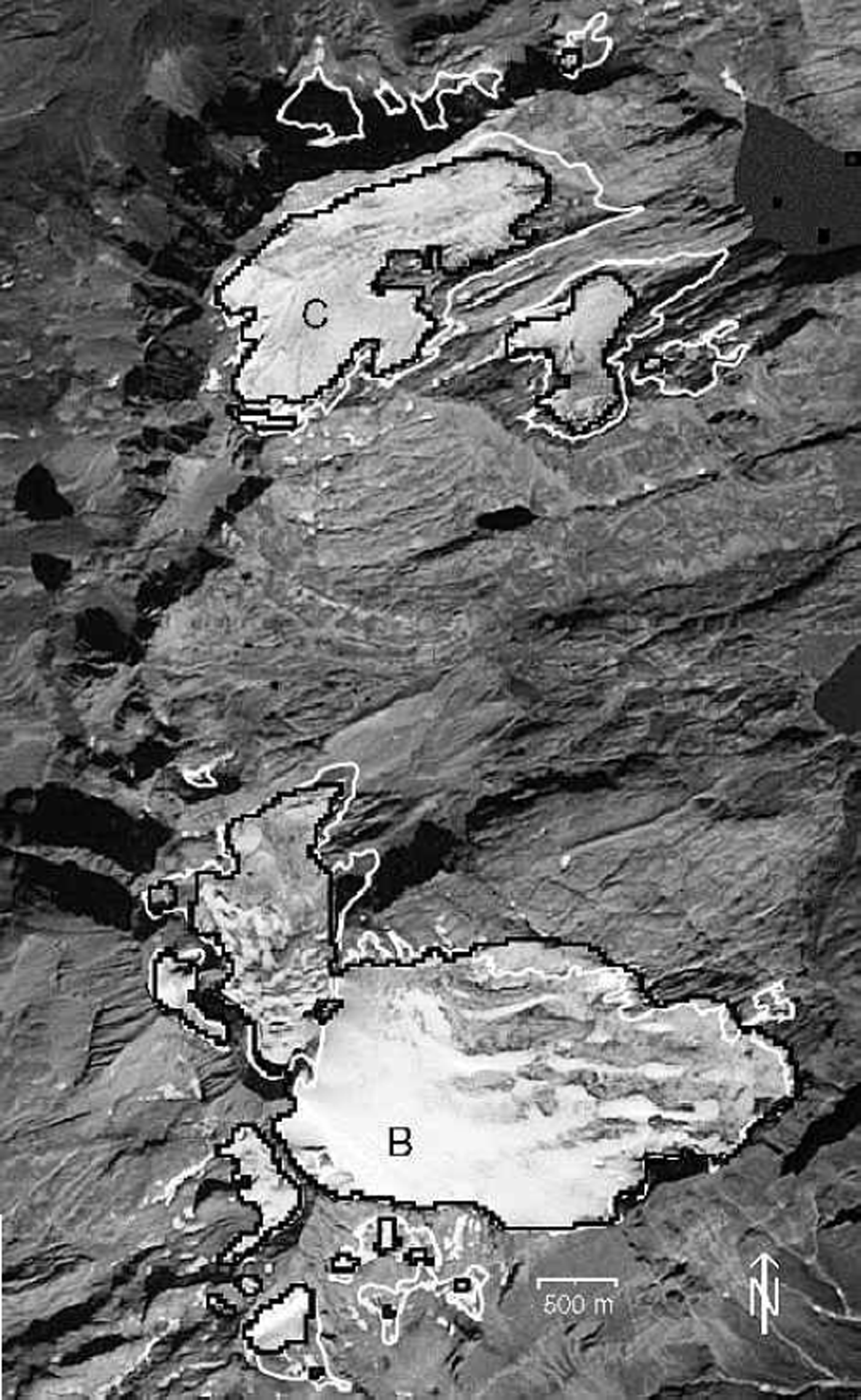
(1) the TM-derived glacier outlines fit quite well to the visible glaciers,
(2) small isolated ice fields are not classified as glaciers,
(3) the smallest glaciers shrank through disintegration into snowpatches,
(4) there is a differentiated retreat of the larger glaciers,
(5) the largest glacier (Basodino) was even larger in 1992 than in 1973.
DEM
Requirements and possibilities
A DEM has two main functions within the SGI 2000: the orthorectification of the satellite imagery, and the derivation of three-dimensional glacier parameters within a GIS. The orthorectification is mandatory for at least four different tasks:
(1) To eliminate the effects of perspective distortion, terrain elevation has to be considered during georectification of imagery of rugged terrain. For instance, a pixel with a height of 3000ma.s.l., located 90 km from the nadir point, is shifted by 370 mfrom its real position in the uncorrected image.
(2) The borders between individual glaciers were assigned to the classified TM image from a (georeferenced) vector layer containing digitized glacier basin outlines.
(3) Overlay of TM scenes from other years or with scenes from other sensors.
(4) Fusion with the DEM itself used to derive glacier parameters.
All scenes for SGI 2000 were orthorectified with a set of ground-control points to a residual rms error of about half a pixel, using a DEM with 25m spatial resolution (SGI 2000 DEM) from the Swiss Federal Office of Topography.
Three-dimensional glacier parameters, like minimum and maximum elevation, glacier length, the median and 2:1 altitude (equilibrium-line altitude), and a detailed hypsography, can be computed automatically with a DEM. Slope and aspect of each glacier can be obtained as an average for the entire glacier or as a percentage of selected zones (e.g. accumulation and ablation area). Moreover, average illumination or the percentage area in cast shadow during a day can be calculated. In this way it is possible to achieve a more thorough understanding of topographic influences on monitored changes in glacier area or length.
Comparison with a reference DEM
To analyze the vertical accuracy of the SGI 2000 DEM, a comparison with a reference DEM directly inferred from stereo-photogrammetry was performed (Reference KääbKääb, 2000). An illuminated version of the SGI 2000 DEM is shown in Figure 4a for a small area (5.7 km by 5.0 km) within the test region. Also indicated are the outlines of seven glaciers, analyzed in the discussion below. Artefacts from the interpolation process between the originally digitized contour lines are visible on the illuminated SGI 2000 DEM. They are notably pronounced in gradient products like slope, as illustrated in Figure 4b, which shows the difference in slope to the reference DEM.
(a) Illuminated version of the DEM used for the SGI 2000 in a subsection of the test area Weissmies with outlines of seven glaciers (numbered) from the digitized inventory of 1973. DEM artefacts are clearly visible. (b) Differences in slope between the DEMin (a) and a reference DEM ranging from –53˚ (black) to +65˚ (white).Most of the artefacts are located outside of glacier areas. Elevation data: DEM 25 © Swiss Office ofTopography (BA013305).
The minimum (maximum) elevation differences are –96 (+74)m for the entire area, with a standard deviation of 8.6 m. The corresponding values for the slope differences are –53 (+60)˚ and 6.6°. Those deviations are not acceptable for the SGI 2000, but the large differences were mostly found at isolated locations or crests, usually not related to glacier coverage. To estimate the influence of the artefacts on the derived glacier parameters, some of them were calculated for the seven glaciers indicated in Figure 4a. The average differences of minimum (maximum) elevation are –2.7 (–1.3)m, with a standard deviation of 7.6 (7.4)m. The corresponding values for slope are 1.2 (–2.5)˚ and 2.4 (3.3)°. These deviations are acceptable for the glacier parameters in the SGI 2000.
GIS
Data preparationsFootnote 1
By using an orthorectified glacier map derived from TM and a suitable DEM, three-dimensional glacier parameters can be obtained automatically within a GIS. Before the GIS-based processing was started, all data products were converted into Arc/Info (ESRI, 1999) specific formats, and three GIS-related tasks were prepared for the SGI 2000:
(1) digitizing of the glacier outlines from the inventory of 1973 into a vector layer,
(2) creation of a vector layer with glacier basin boundaries (see below),
(3) calculation of DEM products (e.g. slope, aspect) for obtaining three-dimensional glacier parameters.
The glacier outlines were digitized from the original maps (scale 1:25 000) as individual arcs, with an average rectification error of each map of about 5 m (rms). The central flowlines and the reconstructed outlines from about 1850 were also digitized.
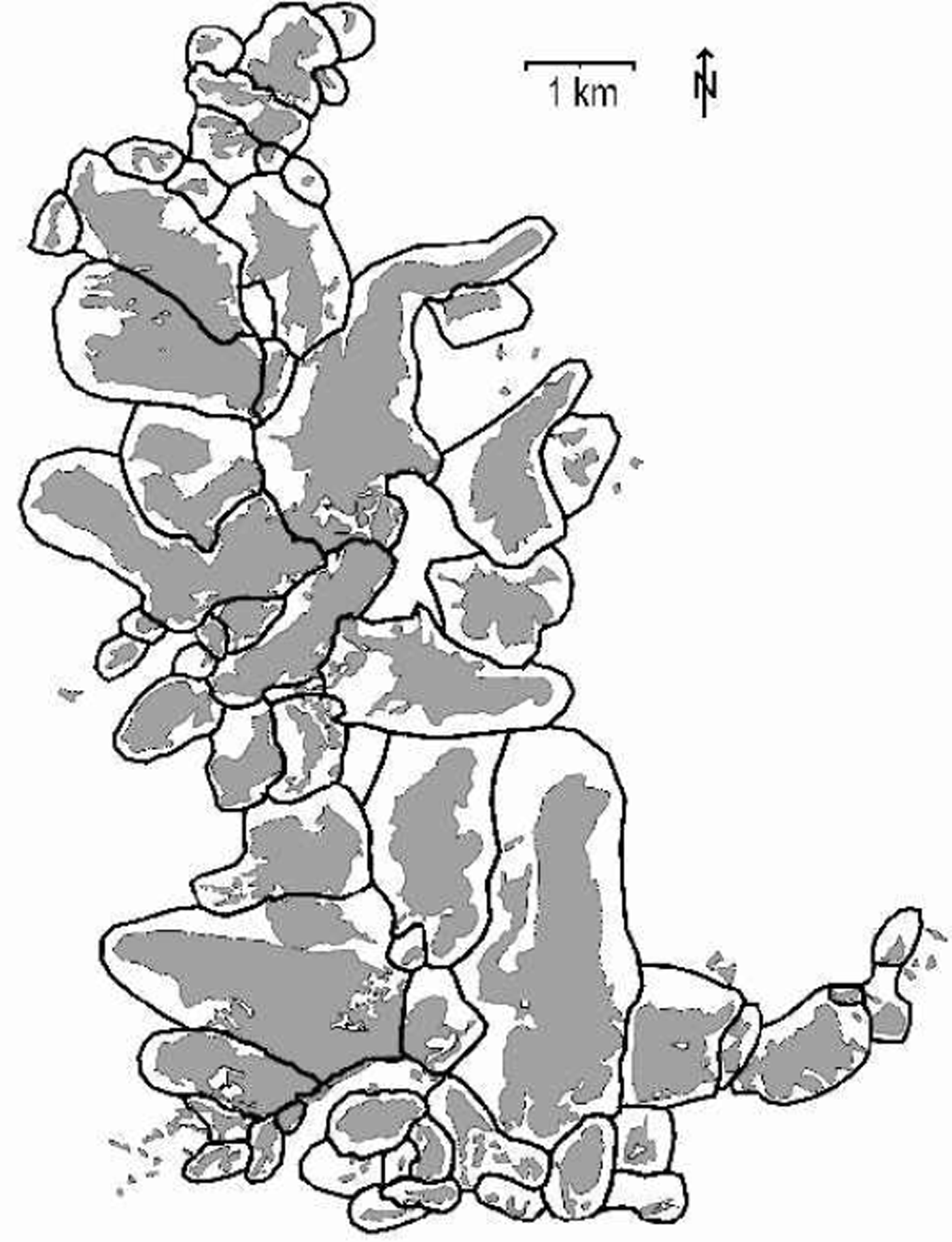
To separate connected glaciers in the classified TM image into individual glaciers, the ice divides between them must be defined. This is done by on-screen digitizing of a new vector layer (coverage) using the digitized Swiss glacier inventory and the classified TM image as background in arcedit. Ice divides were taken without modification from the digitized inventory and extended to a closed polygon roughly surrounding the glacier. All other glaciers were also surrounded by closed polygons, which are large enough to include possible future variations of glacier area. The thick black lines in Figure 5 represent these polygons. They are shown together with the digitized glacier areas (in grey). With these predefined glacier basins it is also possible to assign a unique identity (ID) to glacier groups (see below). A group of glaciers can originate from a single glacier through disintegration over time, already be established in a former inventory or consist of an entire glacier comprised of different streams.
Glacier basins (bold black lines) and the digitized Swiss glacier inventory of 1973 (grey areas). Contiguous ice masses were separated into individual glaciers according to the 1973 inventory, and roughly surrounded to obtain closed polygons. These polygonal glacier basins can also be used to eliminate gross classification errors (e.g. proglacial lakes) and for glacier identification, especially to assign a unique ID to glaciers.
DEM products such as slope or aspect were calculated within the digital image-processing software. Some DEM products are further converted with short FORTRAN programs (e.g. the aspects are classified into eight sectors). The elevation products (e.g. median elevation or hypsography) are computed within Arc/Info.
The location of the glacier ID is taken from the revised database of Reference Maisch, Wipf, Denneler, Battaglia and BenzMaisch and others (1999). Because many glaciers have split up during recent years, the location of their ID (assigned in 1973) often lies outside their present outline. Therefore, and to handle groups of glaciers, the ID is assigned to the entire basin. This is done by converting the database table (ID, x and y-coordinates) to a point coverage with generate and intersecting this coverage with the glacier basin coverage. Thus, each glacier basin holds the glacier ID in the attribute table.
Data flow
The data processing can be separated into a general work flow between three modules and a more specific data flow within each module. The modules are (Fig. 6):
Work flow between sequential modules and principal data flow within each module. In each module different programs are available to calculate glacier parameters and their changes. Most of them can be combined into a complete digital processing chain.
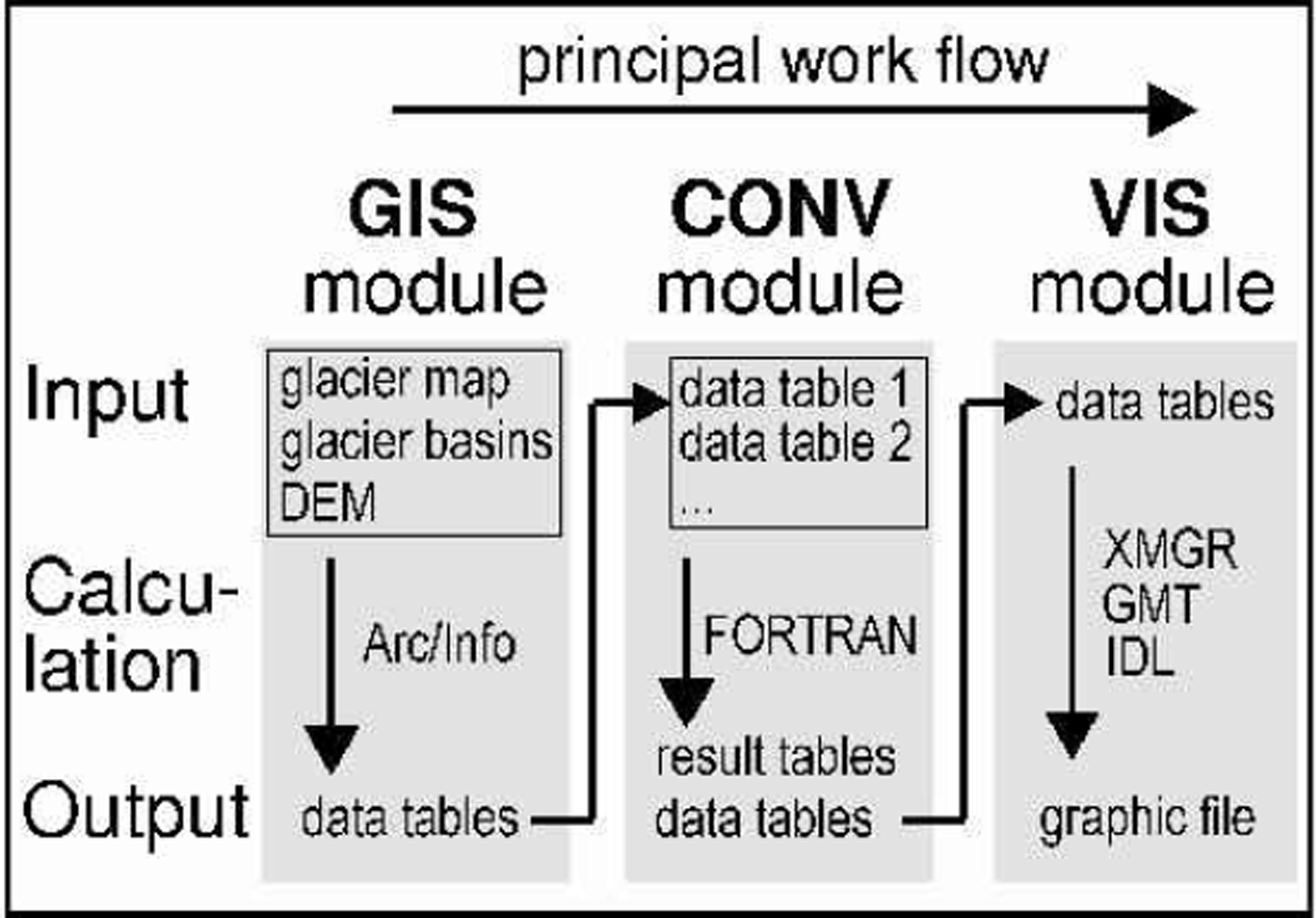
(1) the GIS module for calculating quantities within the GIS (e.g. areas of individual glaciers),
(2) the CONV module for conversion and recalculation of Arc/Info output tables (e.g. glacier areas of two different years into relative changes in area),
(3) the VIS module for creation of graphic files from data files (e.g. with XMGR, GMTor IDL).
Each module holds individual programs for individual tasks, each of which consists of an input, calculation and output part. The different modules can be combined into a complete digital chain, with the output from a program in one module as the input for a program in the next module (cf. Fig. 6).
The GIS module is shown in Figure 7 in more detail. Only three input layers are needed for the GIS module:
The principal data flow within the GIS module using Arc/Info and including a DEM product for three-dimensional glacier parameters. Areas of individual glaciers are available after step 2.
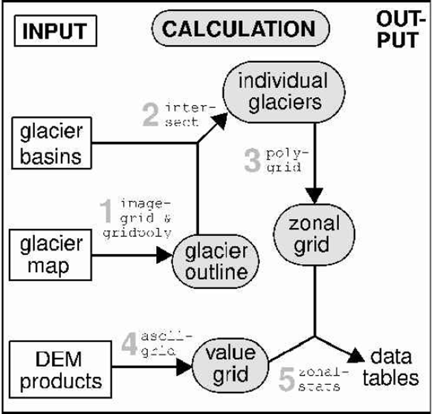
the predefined glacier basins (vector layer) with assigned glacier IDs,
the image with the classified glacier areas from TM
(geo-tiff),
the DEM or a product from it (table with header).
The calculation section consists of the following steps (numbers refer to Fig. 7): The first step (1) is a raster-vector conversion of the glacier map with imagegrid and gridpoly into a coverage. This glacier coverage is then (2) combined with the glacier basin coverage with intersect to obtain the individual glaciers. Together with intersect the glacier basin coverage cuts each glacier out of the glacier coverage in correspondence with its basin. The coverage with the individual glaciers (or a selection of them) is then (3) converted with polygrid to a zonal grid where each zone corresponds to a glacier. The DEM (or a product of it) is (4) converted with asciigrid to a value grid, where each cell holds the value of the DEM at that location. The last step (5) is the combination of the value grid and the zonal grid with zonalstats. This command gives for each zone (glacier) statistic parameters (e.g. minimum, maximum, range, mean, standard deviation) according to the underlying value grid (elevation in case of the DEM). The resulting output table can be processed further with the CONV and VIS modules.
Discussion And Conclusion
The best results for glacier mapping were obtained with thresholding of a TM4 by TM5 ratio image from DN, especially with respect to glacier areas in cast shadow. The accuracy is better than 3% for debris-free glacier areas. Compared to other investigated methods, this method is easy and fast to perform, needs no special image-processing software, and interactive selection of the threshold value is quite robust. The use of a median filter improves the results of the classification by removing misclassification (small snowfields, shadow pixels) and adding pixels where needed (small debris cover, glacier parts in shadow). For glaciers smaller than 0.1km2, the glacier size is altered significantly by this noise filter, and thus the lower limit of total glacier area was determined to be 0.1km2 in the SGI 2000.
The new GIS-based concept of the SGI 2000 is able to compute all glacier parameters automatically. This is very useful for efficient monitoring over large areas, especially in remote regions, or to investigate small glaciers and their changes. The design of the glacier basin vector layer, which maintains the glacier identification, is not limited to the availability of a digitized glacier inventory. In remote areas without any data, creation directly from the satellite image is also possible. If a DEM is available, three-dimensional glacier parameters (e.g. slope, aspect, hypsography) can be calculated automatically, too. For the relatively small glaciers in the Alps, a high-precision DEM with 25 m spatial resolution is necessary for obtaining glacier parameters. Useful data from other regions can also be obtained with a coarser DEM, depending on the size and characteristics of the glaciers considered.
At the moment, the main problem for the SGI 2000 is the automatic mapping of debris-covered glacier ice. It is partly included after the automatic classification (with TM4/TM5) in two cases: the debris cover is thin or it is a medial moraine of only one pixel width (and arbitrary length). In the latter case the median filter will close the gap. Unfortunately, this automatically included part of debris-covered ice has a varying size in different years, depending on snow cover, glacier change or illumination. For this reason, only a small fraction of debris-free glaciers were chosen for comparison of glacier areas in Part II of this paper (Reference Kääb, Paul, Maisch, Hoelzle and HaeberliKääb and others, 2002). A possible solution may be the combination of advanced digital image-processing techniques (neural networks) with geomorphometric measures and object-oriented classification (Reference Bishop, Kargel, Kieffer, MacKinnon, Raup and ShroderBishop and others, 2000). Promising first results have been achieved by combining slope information with a map of vegetation-free areas and neighbourhood relations to glacier ice. Meanwhile, manual delineation by on-screen digitizing is applied for the SGI 2000.
Acknowledgements
The study is supported by a grant from the Swiss National Science Foundation (contract No. 21-54073.98). We gratefully acknowledge the careful and constructive comments of the two anonymous referees and the editor, J. Key.



