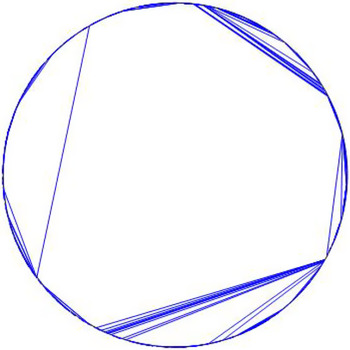
1. Introduction
1.1. Model and motivation
The purpose of this work is to introduce and investigate a geometric representation, as compact subsets of the unit disk, of certain random minimal factorizations of the n-cycle. For an integer
 $n \geq 1$
, let
 $\mathfrak{S}_n$
be the group of permutations of
 $[\![ 1,n ]\!]$
, and
 $\mathfrak{C}_n$
the set of cycles of
 $\mathfrak{S}_n$
. We denote by
 $\ell(c)$
the length of a cycle
 $c \in \mathfrak{C}_n$
. A particular object of interest is the n-cycle
 $c_n \,:\!=\, (1 2 \ldots n)$
, which maps i to
 $i+1$
for
 $1 \leq i \leq n-1$
, and n to 1. For any
 $n \geq k \geq 1$
, the elements of the set
 \begin{align*}\mathfrak{M}_n^{(k)} \,:\!=\, \left\{ (\tau_1, \ldots, \tau_k) \in \mathfrak{C}_n^k, \, \tau_1 \cdots \tau_k = c_n, \, \forall i \, \, \ell(\tau_i) \geq 2, \sum\limits_{i=1}^k \left( \ell(\tau_i)-1 \right) = n-1 \right\}\end{align*}
are called minimal factorizations of
 $c_n$
of order k, while an element of
 \begin{align*}\mathfrak{M}_n \,:\!=\, \underset{k=1}{\overset{n-1}{\bigcup}} \mathfrak{M}_n^{(k)}\end{align*}
is simply called a minimal factorization of
 $c_n$
(one can check that
 $\mathfrak{M}_n^{(k)}$
is empty as soon as
 $k \geq n$
). By convention, we read cycles from the left to the right, so that
 $\tau_1 \tau_2$
corresponds to
 $\tau_2 \circ \tau_1$
. Notice that the condition
 $\sum_{i=1}^k \left( \ell(\tau_i)-1 \right) = n-1$
in the definition of
 $\mathfrak{M}_n^{(k)}$
is a condition of minimality, in the sense that any k-tuple of cycles
 $(\tau_1, \ldots, \tau_k)$
such that
 $\tau_1 \cdots \tau_k = c_n$
necessarily satisfies
 \begin{align*}\sum\limits_{i=1}^k \left( \ell(\tau_i)-1 \right) \geq n-1.\end{align*}
Minimal factorizations of the n-cycle are a topic of interest, mostly in the restrictive case of factorizations into transpositions (that is, all cycles in the factorization have length 2). The number of minimal factorizations of
 $c_n$
into transpositions has been known to be
 $n^{n-2}$
since Dénes [Reference Dénes12], and bijective proofs of this result have been given, for instance by Moszkowski [Reference Moszkowski35] and Goulden and Pepper [Reference Goulden and Pepper21]. These proofs use bijections between the set of minimal factorizations into transpositions and sets of trees, whose cardinality is computed by other means.
More recently, factorizations into transpositions have been studied from a probabilistic perspective by Féray and Kortchemski, who investigate the asymptotic behavior of such a factorization taken uniformly at random, as n grows. On the one hand, they take a ‘local’ point of view [Reference Féray and Kortchemski19], by studying the joint trajectories of finitely many integers through the factorization. On the other hand, they take a ‘global’ point of view [Reference Féray and Kortchemski18], by coding a factorization in the unit disk as was initially suggested by Goulden and Yong [Reference Goulden and Yong20]: associating to each transposition a chord in the disk and drawing these chords in the order in which the transpositions appear in the factorization, they code a uniform factorization by a random process of sets of chords, and prove the convergence of the one-dimensional marginals of this process as n grows, after time renormalization. The author [Reference Thévenin40] extends this result by proving the functional convergence of the whole process, highlighting in addition interesting connections between this model and a fragmentation process of the so-called Brownian continuum random tree (CRT), due to Aldous and Pitman [Reference Aldous and Pitman2]. This fragmentation process codes a way of cutting the CRT at random points into smaller components, as time passes. Being able to obtain such convergence results allows one to understand global properties of a typical large factorization, such as the appearance of ‘large’ transpositions (swapping two integers far from each other).
Let us also mention Angel, Holroyd, Romik and Virág [Reference Angel, Holroyd, Romik and Virág3], and later Dauvergne [Reference Dauvergne11], who investigate from a geometric point of view the closely related model of uniform sorting networks, that is, factorizations of the reverse permutation (which exchanges 1 with n, 2 with
 $n-1$
, etc.) into adjacent transpositions, which exchange only consecutive integers.
In another direction, more general minimal factorizations have been studied as combinatorial structures. Specifically, Biane [Reference Biane5] investigates the case of minimal factorizations of
 $c_n$
of class
 $\overline{a} \,:\!=\, (a_1, \ldots, a_k)$
, where
 $a_1, \ldots, a_k$
are all integers
 $\geq 2$
such that
 $\sum_{i=1}^k (a_i-1) = n-1$
. These factorizations are k-tuples of cycles
 $(\tau_1, \ldots, \tau_k) \in \mathfrak{M}_n^{(k)}$
such that, for
 $1 \leq i \leq k$
,
 $\ell(\tau_i)=a_i$
. Biane proves in particular that, at
 $\overline{a}$
fixed, the number of factorizations of class
 $\overline{a}$
is surprisingly always equal to
 $n^{k-1}$
, and therefore depends only on the cardinality of the class. A proof based on a bijection with a new model of trees is given by Du and Liu [Reference Du and Liu13], which inspired our own bijection, presented in Section 3 and very close to theirs. In particular, the class
 $(2,2,\ldots,2)$
, where 2 is repeated
 $n-1$
times, corresponds to minimal factorizations of the n-cycle into transpositions, and one recovers Dénes’s result. These general minimal factorizations are also related to a multivariate enumeration of Cayley trees [Reference Biane and Josuat-Vergès6]. Let us finally mention the work of Mühle, Nadeau and Williams [Reference Mühle, Nadeau and Williams36], where the authors consider many enumerative properties of the class
 $(k, k, \ldots, k)$
for
 $k \geq 2$
, showing connections between this model, some parking functions, and special instances of the so-called Cambrian lattices.
Our goal in this paper is to extend the geometric approach of uniform minimal factorizations into transpositions initiated by Féray and Kortchemski to minimal factorizations into cycles of random lengths, when the probability of choosing a given factorization depends only on its class.
Weighted minimal factorizations. Let us immediately introduce the object of interest of this paper, which is a new model of random factorizations. The idea is to generalize minimal factorizations of the cycle into transpositions, by giving to each element of
 $\mathfrak{M}_n$
a weight which depends on its class and then choosing a factorization at random proportionally to its weight.
We fix a sequence
 $w \,:\!=\, (w_i)_{i \geq 1}$
of nonnegative real numbers, which we call weights. We will always assume that there exists
 $i \geq 1$
such that
 $w_i>0$
. For any positive integers n, k, and any factorization
 $f \,:\!=\, (\tau_1, \ldots, \tau_k) \in \mathfrak{M}_n^{(k)}$
, we define the weight of f as
 \begin{align*}W_w(f) \,:\!=\, \prod_{i=1}^k w_{\ell(\tau_i)-1}.\end{align*}
Then we define the w-minimal factorization of the n-cycle, denoted by
 $f_n^w$
, as the random variable on the set
 $\mathfrak{M}_n$
such that, for all
 $f \in \mathfrak{M}_n$
, the probability that
 $f_n^w$
is equal to f is proportional to the weight of f:
 \begin{align*}\mathbb{P} \left( f_n^w=f \right) = \frac{1}{Y_{n,w}} W_w(f),\end{align*}
where
 $Y_{n,w} \,:\!=\, \sum_{f \in \mathfrak{M}_n} W_w(f)$
is a renormalization constant. We shall implicitly restrict our study to the values of n such that
 $Y_{n,w}>0$
.
Note that some particular weight sequences give birth to specific models of random factorizations:
-
Fix an integer
 $r \geq 2$
, and define
$\delta^r$
as follows:
$\delta^r_{r-1}=1$
, and for all
$k \neq r-1$
,
$\delta^r_k=0$
. In this case,
$f_n^{\delta^r}$
is a uniform minimal factorization of the n-cycle into r-cycles. In particular, when
$r=2$
, one recovers the model of minimal factorizations into transpositions, studied in depth in [Reference Féray and Kortchemski18, Reference Féray and Kortchemski19, Reference Thévenin40].
-
Define v as the weight sequence such that, for all
$k \geq 1$
,
$v_k=1$
. In this case,
$f_n^v$
is a uniform element of
$\mathfrak{M}_n$
.


Minimal factorizations of stable type. We specifically focus in this paper on a particular case of weighted factorizations, which we call factorizations of stable type. These random factorizations of the n-cycle are of great interest, as we can code them by a process of compact subsets of the unit disk which converges in distribution (see Theorem 1.1).
Let us start with some definitions. A function
 $L\,:\, \mathbb{R}_+^* \rightarrow \mathbb{R}_+^*$
is said to be slowly varying if, for any
 $c>0$
,
 $L(cx)/L(x) \rightarrow 1$
as
 $x \rightarrow \infty$
. For
 $\alpha \in (1,2]$
, we say that a probability distribution
 $\mu$
which is critical—that is,
 $\mu$
has mean 1—is in the domain of attraction of an
 $\alpha$
-stable law if there exists a slowly varying function L such that, as
 $x \rightarrow \infty$
,
 \begin{equation}Var\left[ X \, \unicode{x1D7D9}_{X \leq x} \right] \sim x^{2-\alpha} L(x),\end{equation}
where X is a random variable distributed according to
 $\mu$
. We refer to [Reference Janson22] for an in-depth study of these well-known distributions. In particular, any law with finite variance is in the domain of attraction of a 2-stable law.
Throughout the paper, for such a distribution
 $\mu$
,
 $(B_n)_{n \geq 1}$
denotes a sequence of positive real numbers satisfying
 \begin{equation}\frac{n L(B_n)}{B_n^\alpha} \underset{n \rightarrow \infty}{\rightarrow} \frac{\alpha (\alpha - 1)}{\Gamma \left( 3 - \alpha \right)},\end{equation}
where L satisfies (1.1). Notice in particular that if
 $\mu$
has finite variance
 $\sigma^2$
, then
 $L(x) \rightarrow \sigma^2$
as
 $x \rightarrow \infty$
, and (1.2) can be rewritten as
 $\smash{B_n \underset{n \rightarrow \infty}{\sim} \frac{\sigma}{\sqrt{2}} \sqrt{n}}$
. For such a sequence
 $(B_n)_{n \geq 1}$
, we denote by
 $(\tilde{B}_n)_{n \geq 1}$
the sequence defined as
 \begin{equation}\tilde{B}_n = \left\{ \begin{aligned} B_n \qquad & \text{ if } \quad \alpha<2, \text{ or } \alpha=2 \text{ and } Var(\mu)=\infty,\\[5pt] \sqrt{\frac{\sigma^2+1}{2}} \sqrt{n} \qquad & \text{ if } \quad Var(\mu) = \sigma^2<\infty. \\ \end{aligned} \right.\end{equation}
Finally, for
 $\alpha \in (1,2]$
, we say that a weight sequence w is of
 $\alpha$
-stable type if there exist a critical distribution
 $\nu$
defined on the set
 $\mathbb{Z}_+ \,:\!=\, \{ 0,1,2,\ldots \}$
of natural integers in the domain of attraction of an
 $\alpha$
-stable law and a real number
 $s>0$
such that, for all
 $i \geq 1$
,
 \begin{align*}w_i = \nu_i s^i.\end{align*}
Notice that this condition concerns only
 $i \geq 1$
, and thus
 $\nu_0$
can be seen as a ‘free parameter’. In this case,
 $\nu$
is said to be the critical equivalent of w. One can check that, if w admits a critical equivalent—which is not always the case—then it is unique. Furthermore, it appears that, whenever different weight sequences may have the same critical equivalent, the distribution of the minimal factorization
 $f_n^w$
depends only on this critical law. If w is a weight sequence of
 $\alpha$
-stable type, then we also say that
 $f_n^w$
is a minimal factorization of
 $\alpha$
-stable type.
Throughout the paper, we investigate several combinatorial quantities of these factorizations. Here are two examples. As a first result, we can control the number of cycles in such a factorization. For any
 $n \geq 1$
and any minimal factorization F of the n-cycle, denote by N(F) the number of cycles in F.
Proposition 1.1. Let w be a weight sequence of
 $\alpha$
-stable type for some
 $\alpha \in (1,2]$
, and let
 $\nu$
be its critical equivalent. Then, as
 $n \rightarrow \infty$
,
 \begin{equation*}\frac{1}{n} N \left( f_n^w \right) \overset{\mathbb{P}}{\rightarrow} 1-\nu_0,\end{equation*}
where
 $\overset{\mathbb{P}}{\rightarrow}$
denotes convergence in probability.
In words, the number of cycles in
 $f_n^w$
behaves linearly in n. The proof of this lemma can be found in Section 3.3, and is an immediate corollary of Theorem 3.3 and Lemma 4.2.
Example 1.1. If one looks at the weight sequence v defined as
 $v_i=1$
for all
 $i \geq 1$
(so that
 $f_n^v$
is a uniform element of
 $\mathfrak{M}_n$
), then one can check that v has a critical equivalent
 $\nu$
satisfying
 $\nu_0 = (3-\sqrt{5})/2$
and
 $\nu_i = ((3-\sqrt{5})/2)^i$
for
 $i \geq 1$
. Thus, the average number of cycles in a uniform minimal factorization of the n-cycle is of order
 $(1-\nu_0) n = (\sqrt{5}-1) \, n/2$
.
As another side result, we are able to control the length of the largest cycle in such factorizations. For any
 $n \geq 1$
and any minimal factorization F of the n-cycle, denote by
 $\ell_{max}(F)$
the length of the largest cycle in F.
Proposition 1.2. Let w be a weight sequence of
 $\alpha$
-stable type for some
 $\alpha \in (1,2]$
, and let
 $\nu$
be its critical equivalent. For any sequence
 $(B_n)_{n \geq 1}$
satisfying (1.2) for
 $\nu$
, the following hold:
-
(i) if
$\alpha = 2$
, then with probability going to 1 as
$n \rightarrow \infty$
,
$\ell_{max}(f_n^w) = o(B_n)$
; -
(ii) if
$\alpha<2$
, then for any
$\epsilon>0$
there exists
$\eta>0$
such that, for n large enough, with probability larger than
$1-\epsilon$
,
$\eta B_n \leq \ell_{max}(f_n^w) \leq \eta^{-1} B_n$
.


In other words, for
 $\alpha<2$
, the largest cycle in
 $f_n^w$
is of order
 $B_n$
(thus of order
 $n^{1/\alpha}$
, up to a slowly varying function). If
 $\alpha=2$
then one can only say that the largest cycle is of length
 $o(B_n)$
(which means
 $o(\sqrt{n})$
if
 $\nu$
has finite variance). This is proved in Section 4.1.
1.2. Coding a minimal factorization by a colored lamination-valued process
The first aim of this paper is to code random minimal factorizations in the unit disk. In what follows,
 $\overline{\mathbb{D}} \,:\!=\, \{ z \in \mathbb{C}, |z| \leq 1 \}$
denotes the closed unit disk and
 $\mathbb{S}^1 \,:\!=\, \{ z \in \overline{\mathbb{D}}, |z|=1 \}$
the unit circle.
The idea of coding random structures by compact subsets of
 $\overline{\mathbb{D}}$
goes back to Aldous [Reference Aldous1], who investigates triangulations of large polygons: let
 $n \in \mathbb{Z}_+$
and define
 $P_n$
to be the regular n-gon inscribed in
 $\overline{\mathbb{D}}$
whose vertices are
 $\left\{ e^{2i k\pi/n}, 1 \leq k \leq n \right\}$
. Aldous proves that a random uniform triangulation of
 $P_n$
(that is, a set of non-crossing diagonals of
 $P_n$
whose complement in
 $P_n$
is a union of triangles) converges in distribution towards a random compact subset of the disk which he calls the Brownian triangulation. This Brownian triangulation is in particular a lamination—that is, a compact subset of
 $\overline{\mathbb{D}}$
made of the union of the circle and a set of chords that do not intersect, except maybe at their endpoints. In particular, the faces of this lamination, which are the connected components of its complement in
 $\overline{\mathbb{D}}$
, are all triangles. See Figure 1, middle, for a simulation of this lamination. Since the work of Aldous, the Brownian triangulation has appeared as the limit of various random discrete structures [Reference Bettinelli4, Reference Curien and Kortchemski10], and has also been connected to random maps [Reference Le Gall and Paulin31].
Left: a simulation of the
 $1.3$
-stable lamination
 $\mathbb{L}_\infty^{(1.3)}$
. Middle: a simulation of the Brownian triangulation
 $\mathbb{L}_\infty^{(2)}$
. Right: a simulation of
 $\mathbb{L}_\infty^{(2),0.5}$
.

In a extension of Aldous’s work, Kortchemski [Reference Kortchemski28] constructed a family
 $(\mathbb{L}_\infty^{(\alpha)})_{1<\alpha \leq 2}$
of random laminations, called
 $\alpha$
-stable laminations (see Figure 1, left, for a simulation of the stable lamination
 $\mathbb{L}^{(1.3)}$
). These laminations appear as limits of large general Boltzmann dissections of the regular n-gon [Reference Kortchemski28]. This extends Aldous’s result about triangulations, since the 2-stable lamination
 $\mathbb{L}_\infty^{(2)}$
is distributed as the Brownian triangulation. Stable laminations are also limits of large non-crossing partitions [Reference Kortchemski and Marzouk29].
Let us now introduce colored laminations, which generalize the notion of lamination. A colored lamination is a subset of
 $\overline{\mathbb{D}}$
in which each point is either colored black or red, or left white, so that the subset of red points is a lamination whose faces are each either completely black or completely white. (See Figure 2 for an example.) A particular example of colored laminations is the colored analogue of the
 $\alpha$
-stable laminations. These objects are colored laminations whose red chords form the
 $\alpha$
-stable lamination, and whose faces are colored black in an independent and identically distributed (i.i.d.) way. Specifically, for
 $p \in [0,1]$
, the p-colored
 $\alpha$
-stable lamination
 $\mathbb{L}_\infty^{(\alpha),p}$
is a random colored lamination such that (i) the red part of
 $\mathbb{L}_\infty^{(\alpha),p}$
has the law of
 $\mathbb{L}_\infty^{(\alpha)}$
, and (ii) independently of the red component, the faces of
 $\mathbb{L}_\infty^{(\alpha),p}$
are colored black independently of each other with probability p
 $\big($
see Figure 1, right, for a simulation of
 $\mathbb{L}_\infty^{(2), 0.5}\big)$
.
The subset S(f) where
 $f \,:\!=\, (5678)(23)(125)(45)$
is an element of
 $\mathfrak{M}_8$
.

We now provide a way of representing a minimal factorization by a process of colored laminations of the unit disk. This representation is a generalization of the representation of a minimal factorization into transpositions, introduced by Goulden and Yong [Reference Goulden and Yong20]. It consists in drawing, for each cycle
 $\tau$
of the factorization, a number
 $\ell(\tau)$
of red chords in
 $\overline{\mathbb{D}}$
, and coloring the face that it creates in black. More precisely, for
 $n \geq 1$
, let
 $\tau \in \mathfrak{C}_n$
be a cycle and assume that it can be written as
 $(e_1, \ldots, e_{\ell(\tau)})$
, where
 $e_1 < \cdots < e_{\ell(\tau)}$
. We will prove later that indeed, if
 $\tau$
appears in a minimal factorization of the n-cycle, then it satisfies this condition (see Section 3 for details and proofs). Then draw in red, for each
 $1 \leq j \leq \ell(\tau)-1$
, the chord
 $[e^{-2i \pi e_j/n}, e^{-2i \pi e_{j+1}/n}]$
, and also draw the chord
 $[e^{-2i \pi e_{\ell(\tau)}/n}, e^{-2i \pi e_1/n}]$
(here, [x, y] denotes the segment connecting x and y in
 $\mathbb{R}^2$
). This creates a red cycle. Color now the interior of this cycle in black, and finally color the unit circle in red. We denote the colored lamination that we obtain by
 $S(\tau)$
.
Now, let
 $n, k \geq 1$
and
 $f \,:\!=\, (\tau_1,\ldots,\tau_k) \in \mathfrak{M}_n^{(k)}$
. For
 $c \in [0,\infty]$
, define
 $S_c(f)$
as the colored lamination
 \begin{align*}S_c(f) = \mathbb{S}^1 \cup \bigcup_{r=1}^{\lfloor c \rfloor \wedge k} S(\tau_r),\end{align*}
and finally define S(f) as
 $S(f) \,:\!=\, S_k(f) = \bigcup_{r=1}^k S(\tau_r)$
. See Figure 2 for an example.
In their study of a uniform minimal factorization of the n-cycle into transpositions (which we now denote by
 $f_n^{(2)}$
instead of
 $f_n^{\delta^2}$
, for convenience), Féray and Kortchemski [Reference Féray and Kortchemski18] show that a phase transition appears after having read roughly
 $\sqrt{n}$
transpositions. Specifically, at
 $c \geq 0$
fixed, the lamination
 $S_{c \sqrt{n}}(f_n^{(2)})$
converges in distribution for the Hausdorff distance, as n grows, to a random lamination
 $\mathbb{L}_c^{(2)}$
. The author [Reference Thévenin40] later obtains the functional analogue of this convergence, thus providing a coupling between the laminations
 $(\mathbb{L}^{(2)}_c)_{c \geq 0}$
. Let us explain in which sense we understand the convergence of colored lamination-valued processes: for E, F two metric spaces, following Annex A2 in [Reference Kallenberg24], let
 $\mathbb{D}(E,F)$
be the space of càdlàg functions from E to F (that is, right-continuous functions with left limits), endowed with the
 $J_1$
Skorokhod topology. In our case, we see a colored lamination of
 $\overline{\mathbb{D}}$
as an element of
 $\mathbb{K}^2$
, where
 $\mathbb{K}$
denotes the space of compact subsets of
 $\mathbb{D}$
. The first coordinate corresponds to the set of red points, which is a lamination by definition, and the second one to the colored component (the set of points that are black or red). Finally, the set
 $\mathbb{CL}(\overline{\mathbb{D}})$
of colored laminations of
 $\overline{\mathbb{D}}$
is endowed with the Haudsorff distance on the product space
 $\mathbb{K}^2$
, which we denote by
 $d_H$
. Finally, the set of laminations of the disk is seen as a subset of
 $\mathbb{CL}(\overline{\mathbb{D}})$
, on which the red part and the colored part of an element are equal.
Theorem. ([Reference Thévenin40, Theorem 1.2].) There exists a lamination-valued process
 $(\mathbb{L}^{(2)}_c)_{c \in [0,\infty]}$
such that the following convergence holds in distribution for the Skorokhod distance in
 $\mathbb{D}([0,\infty], \mathbb{CL}(\overline{\mathbb{D}}))$
, as
 $n \rightarrow \infty$
:
 \begin{equation}\left( S_{c \sqrt{n}}\left(f_n^{(2)} \right) \right)_{c \in [0,\infty]} \overset{(d)}{\rightarrow} \left( \mathbb{L}^{(2)}_c \right)_{c \in [0,\infty]}.\end{equation}
In this case, it is to be noted that no face with three or more chords in its boundary appears in
 $S(f_n^{(2)})$
, as
 $S(\tau)$
is in fact just the union of
 $\mathbb{S}^1$
and a chord when
 $\ell(\tau)=2$
. Therefore, no point of
 $S(f_n^{(2)})$
is black, and for any
 $c \in [0,\infty]$
,
 $S_{c\sqrt{n}}(f_n^{(2)})$
is just a lamination. Moreover, it appears that the process
 $(\mathbb{L}^{(2)}_c)_{c \in [0,\infty]}$
is a nondecreasing interpolation between the unit circle and the Brownian triangulation.
Our main result, which generalizes (1.4), states the convergence of the geometric representation of a random minimal factorization of stable type. In the stable case, the phase transition does not appear at the scale
 $\sqrt{n}$
anymore, but at the scale
 $\tilde{B_n}$
.
Theorem 1.1. Let
 $\alpha \in (1,2]$
and w a weight sequence of
 $\alpha$
-stable type. Let
 $\nu$
be its critical equivalent, and let
 $(\tilde{B}_n)_{n \geq 0}$
satisfy (1.3). Then there exists a lamination-valued process
 $(\mathbb{L}_c^{(\alpha)})_{c \in [0,\infty]}$
, depending only on
 $\alpha$
, such that the following hold:
-
(I) If
$\alpha<2$
, then the following convergence holds:
\begin{align*}\left( \left( S_{c (1-\nu_0) \tilde{B}_n}(f_n^w) \right)_{0 \leq c < \infty}, S_\infty(f_n^w) \right) \underset{n \rightarrow \infty}{\overset{(d)}{\rightarrow}} \left( \left(\mathbb{L}_c^{(\alpha)} \right)_{0 \leq c < \infty}, \mathbb{L}_\infty^{(\alpha), 1}\right).\end{align*}
-
(II) If
$\nu$
has finite variance, there exists a parameter
$p_\nu \in [0,1]$
such that the following convergence holds: Furthermore,
\begin{align*}\left( \left( S_{c (1-\nu_0) \tilde{B}_n}(f_n^w) \right)_{0 \leq c < \infty}, S_\infty(f_n^w) \right) \underset{n \rightarrow \infty}{\overset{(d)}{\rightarrow}} \left( \left(\mathbb{L}_c^{(2)} \right)_{0 \leq c < \infty}, \mathbb{L}_\infty^{(2), p_\nu}\right).\end{align*}
where
\begin{align*}p_\nu = \frac{\sigma_\nu^2}{\sigma_\nu^2+1},\end{align*}
$\sigma_\nu^2$
denotes the variance of
$\nu$
.


Both convergences hold in distribution in the space
 $\mathbb{D}(\mathbb{R}_+, \mathbb{CL}(\overline{\mathbb{D}})) \times \mathbb{CL}(\overline{\mathbb{D}})$
.
This process
 $(\mathbb{L}_c^{(\alpha)})_{c \in [0,\infty]}$
is a nondecreasing interpolation between the circle and
 $\mathbb{L}_\infty^{(\alpha)}$
. It is in addition lamination-valued, in the sense that, for all
 $c \geq 0$
, almost surely
 $\mathbb{L}_c^{(\alpha)}$
contains no black point.
Roughly speaking, this geometric representation provides a way of defining the ‘scaling limit’ of a minimal stable-type factorization of the n-cycle. This convergence result makes it possible to capture information about a typical such factorization, such as the largest distance between two integers in a cycle or the time at which large cycles appear in the factorization. In addition, it shows the universality of the limiting objects, in the sense that they are the limits of different stable-type factorizations.
Notice that Theorem 1.1 is an extension of [Reference Thévenin40, Theorem 3.3]. However this generalization is not straightforward at all. In particular, we need to introduce a new bijection between general minimal factorizations and conditioned bi-type trees in order to understand the asymptotic structure of the colored laminations. Thus, proving that black faces appear at
 $c=\infty$
in the colored lamination-valued process requires a refined investigation of asymptotic properties of these conditioned bi-type trees, whose study is more complex than in the monotype case. In particular a new shuffling operation on vertices (Definition 4.1) is needed.
Remark 1.1. We conjecture that the result of Theorem 1.1(I) still holds when
 $\alpha=2$
and
 $\nu$
has infinite variance. However, our proofs do not directly apply to this case.
Example 1.2. In the case
 $w = \delta^j$
for some
 $j \geq 1$
, the critical equivalent of
 $\delta^j$
is
 $\nu \,:\!=\, \frac{j-2}{j-1} \delta^0 + \frac{1}{j-1} \delta^j$
, and
 $p_\nu=\frac{j-2}{j-1}$
. When
 $j=2$
,
 $p_\nu=0$
and we recover the Brownian triangulation without coloration, as the limit of the lamination obtained from a uniform minimal factorization of the n-cycle into transpositions. In the case
 $j=3$
of factorizations into 3-cycles, each face of the limiting colored Brownian triangulation is black with probability
 $1/2$
.
In the case of a minimal factorization of the n-cycle taken uniformly at random, one obtains the surprising limit value
 $p_\nu=1-1/\sqrt{5}$
.
Remark 1.2. Using the same tools as for the proof of Theorem 1.1, one can prove that the following slightly stronger convergence holds in the space
 $\mathbb{D}(\mathbb{R}_+, \mathbb{CL}(\overline{\mathbb{D}})) \times \mathbb{D}((0,1], \mathbb{CL}(\overline{\mathbb{D}}))$
:
-
(i) If
$\alpha<2$
,
\begin{align*}\left( \left( S_{c (1-\nu_0) \tilde{B}_n}\left(f_n^w\right) \right)_{0 \leq c < \infty}, \left(S_{dn}\left(f_n^w\right) \right)_{0 < d \leq 1} \right) \underset{n \rightarrow \infty}{\overset{(d)}{\rightarrow}} \left( \left(\mathbb{L}_c^{(\alpha)} \right)_{0 \leq c < \infty}, \left( \mathbb{L}_{\infty}^{(\alpha),d} \right)_{0 < d \leq 1} \right).\end{align*}
-
(ii) If
$\nu$
has finite variance, then
\begin{align*}\left( \left( S_{c (1-\nu_0) \tilde{B}_n}\left(f_n^w\right) \right)_{0 \leq c < \infty}, \left( S_{dn}\left(f_n^w\right) \right)_{0 < d \leq 1} \right) \underset{n \rightarrow \infty}{\overset{(d)}{\rightarrow}} \left( \left(\mathbb{L}_c^{(2)} \right)_{0 \leq c < \infty}, \left( \mathbb{L}_{\infty}^{(2), d p_\nu} \right)_{0 < d \leq 1} \right).\end{align*}


Here, for
 $p \in [0,1]$
and
 $\alpha \in (1,2]$
, the process
 $\left( \mathbb{L}_{\infty}^{(\alpha), dp} \right)_{0 < d \leq 1}$
that appears at the limit interpolates in a ‘linear’ way between the stable lamination
 $\mathbb{L}_\infty^{(\alpha)}$
(for
 $d \downarrow 0$
) and the colored stable lamination
 $\mathbb{L}_\infty^{(\alpha),p}$
(for
 $d=1$
). In words, the faces that are colored in the limiting lamination
 $\mathbb{L}_\infty^{(\alpha),p}$
appear in the process at independent times
 $Y_i n$
, where the
 $Y_i$
are uniform on (0,1]. In some sense, this marks a second phase transition at scale n, in which large black faces begin to appear.
1.3. Construction of the processes
$(\mathbb{L}_c^{(\alpha)})_{c \in [0,\infty]}$

Let us immediately explain how to construct the limiting processes
 $(\mathbb{L}_c^{(\alpha)})_{c \in [0,\infty]}$
which appear in the statement of Theorem 1.1 and in (1.4). In order to understand this construction, we define from a (deterministic) càdlàg function
 $F: [0,1] \rightarrow \mathbb{R}_+$
such that
 $F(0)=F(1)=0$
a random lamination-valued process
 $(\mathbb{L}_c(F))_{c \in [0,\infty]}$
. Define the epigraph of F as
 $\mathcal{EG}(F) \,:\!=\, \{ (s,t) \in \mathbb{R}^2, 0 \leq s \leq 1, \, 0 \leq t \lt F(s) \}$
, the set of all points that are under the graph of F. Denote by
 $\mathcal{P}(F)$
an inhomogeneous Poisson point process on
 $\mathcal{EG}(F) \times \mathbb{R}_+$
, of intensity
 \begin{align*}\frac{ds dt}{d(F,s,t)-g(F,s,t)} \unicode{x1D7D9}_{(s,t) \, \in \, \mathcal{EG}(F)} \, dr,\end{align*}
where
 $g(F,s,t) \,:\!=\, \sup \{ s' \leq s, F(s') < t \}$
and
 $d(F,s,t) \,:\!=\, \inf \{ s' \geq s, F(s') < t \}$
, and r is to be understood as a ‘time’ coordinate. For any
 $c \geq 0$
, its restriction to
 $\mathbb{R}^2 \times [0,c]$
is denoted by
 $\mathcal{P}_c(F)$
. Now, for
 $c \geq 0$
, define the lamination
 $\mathbb{L}_c(F)$
as
 \begin{align*}\mathbb{S}^{1} \cup \overline{\bigcup\limits_{(s,t) \in \mathcal{P}_c(F)} \left[e^{-2i\pi g(F,s,t)}, e^{-2i\pi d(F,s,t)}\right]},\end{align*}
so that each point of
 $\mathcal{P}_c(F)$
codes a chord in
 $\overline{\mathbb{D}}$
(see Figure 3), and let
 $\mathbb{L}_\infty(F)$
be the lamination
 $\overline{\bigcup_{c \geq 0} \mathbb{L}_c(F)}$
.
A càdlàg function F, a point (s, t) of its epigraph
 $\mathcal{EG}(F)$
, and the corresponding chord in
 $\overline{\mathbb{D}}$
.

For
 $\alpha \in (1,2]$
, the process
 $(\mathbb{L}_c^{(\alpha)})_{c \in [0,\infty]}$
is constructed this way from the so-called stable height process
 $H^{(\alpha)}$
:
 \begin{align*}\left(\mathbb{L}_c^{(\alpha)}\right)_{c \in [0,\infty]} = \left(\mathbb{L}_c\left(H^{(\alpha)}\right)\right)_{c \in [0,\infty]}.\end{align*}
These stable height processes are random continuous processes on [0,1], and can be defined starting from stable Lévy processes (see Figure 4, right, for a simulation of
 $H^{(1.7)}$
, and Section 2 for more background and details). Figure 5 shows an approximation of the lamination
 $\mathbb{L}^{(1.8)}_15$
.
A simulation of the normalized Brownian excursion
 $\unicode{x1D556}$
(left) and the
 $1.7$
-stable height process
 $H^{(1.7)}$
(right).

A simulation of the lamination
 $\mathbb{L}^{(1.8)}_{15}$
.

In the case
 $\alpha=2$
, the 2-stable height process happens to be distributed as the normalized Brownian excursion
 $(\unicode{x1D556}_t)_{0 \leq t \leq 1}$
, which is roughly speaking a Brownian motion between 0 and 1, conditioned to reach 0 at time 1 and to be nonnegative between 0 and 1 (see Figure 4, left, for a simulation of
 $\unicode{x1D556}$
). It appears in addition that the lamination
 $\mathbb{L}_\infty^{(2)}$
coded by
 $\unicode{x1D556}$
has the law of Aldous’s Brownian triangulation.
1.4. A bijection with labeled bi-type trees
The main idea in the proof of Theorem 1.1 is to use a bijection between the set of minimal factorizations of the n-cycle and a certain set of discrete trees with labels on their vertices. Specifically, for
 $n \geq 1$
, denote by
 $\mathfrak{U}_{n}$
the set of trees T that satisfy the following conditions:
-
T is a bi-type tree; that is, its vertices at even height are colored white and its vertices at odd height are colored black.
-
The root and the leaves of T are white. In other words, each black vertex necessarily has at least one child.
-
T has n white vertices.
-
Black vertices of T are labeled from 1 to
$N^\bullet(T)$
, where
$N^\bullet(T)$
is the total number of black vertices in the tree. In addition, the labels of the neighbors (parent and children) of each white vertex are sorted in decreasing clockwise order, starting from the neighbor with maximum label, and the labels of the children of the root are sorted in decreasing order from left to right.


See Figure 6 for an example.
An element of the set
 $\mathfrak{U}_{13}$
. Its nine black vertices are labeled from 1 to 9, in clockwise decreasing order around each white vertex. The children of the root are in decreasing order.

Theorem 1.2. For any
 $n \geq 1$
, the sets
 $\mathfrak{M}_n$
and
 $\mathfrak{U}_n$
are in bijection.
Let us explain our bijection, whose details and proof can be found in Section 3. Roughly speaking, from a minimal factorization
 $f \in \mathfrak{M}_n$
, one constructs
 $T(f) \in \mathfrak{U}_n$
as the ‘dual tree’ of the colored lamination S(f): one puts a black vertex in each black face or lone chord and a white vertex in each white face, connecting two vertices if the corresponding faces are neighbors. Then, root the obtained tree in the white vertex whose face contains the arc between 1 and n, and label black vertices in the order in which the corresponding faces appear in the process. See Figure 7 for an example of this bijection.
An application of our bijection to the minimal factorization
 $f \,:\!=\, (5678)(23)(125)(45) \in \mathfrak{M}_8$
. Top left: the colored lamination S(f), whose labeled black faces are labeled in the order of the corresponding cycles. Top right: the same lamination, with its dual tree T(f) drawn in blue. The larger white vertex is its root. Bottom: the dual tree T(f) alone.

Notice that this bijection is particularly well suited to tracking some global properties of factorizations. For instance, a key observation in the proof of Proposition 1.1 is that the maximum size of a cycle in a factorization is coded by the maximum degree of a black vertex in the corresponding tree. As another example, the colors of the faces in the asymptotic colored laminations in Theorem 4.1 can be seen on the bi-type trees, and are related to the local structure of its branching points.
Using this bijection, Theorem 1.1 is therefore obtained as a corollary of a similar result on trees that states the convergence of colored lamination-valued processes coding random bi-type trees (Theorem 4.1). Indeed it appears that, when w is a weight sequence of stable type, the random bi-type tree
 $T(f_n^w)$
is distributed as a size-conditioned multitype Galton–Watson tree, whose structure is well understood (see e.g. [Reference Miermont34, Reference Ojeda38]).
Notation. Throughout the paper,
 $\overset{\mathbb{P}}{\rightarrow}$
denotes convergence in probability,
 $\overset{(d)}{\rightarrow}$
convergence in distribution, and
 $\overset{(d)}{=}$
equality in distribution. Moreover, a sequence of events
 $(E_n)_{n \geq 0}$
being given, we say that
 $E_n$
occurs with high probability if
 $\mathbb{P}(E_n) \rightarrow 1$
as
 $n \rightarrow \infty$
. Finally, throughout the paper,
 $\mu_*$
denotes the Poisson distribution with parameter 1.
Outline of the paper. In Section 2, we define and investigate plane trees and more particularly bi-type trees, which are a cornerstone of the paper as they code minimal factorizations, and we suggest two different ways of coding bi-type trees by colored lamination-valued processes. Next, in Section 3, we investigate in depth the model of minimal factorizations and exhibit a natural bijection between the sets
 $\mathfrak{M}_n$
and
 $\mathfrak{U}_n$
for all n. The goal of Section 4 is to prove the convergence of one of the colored lamination-valued processes coding a random bi-type tree (Theorem 4.1), this bi-type tree being the image of a weighted minimal factorization by the abovementioned bijection. This result concerns only trees and may be of independent interest. Finally, Section 5 is devoted to the proof of Theorem 1.1. To this end, we prove that the process of colored laminations coding a minimal factorization and the one coding its image by the bijection are close to each other, before using the result of Section 4.
2. Plane trees, bi-type trees, and different ways of coding them by laminations
In this section, we rigorously define our notion of trees. We then describe a certain family of trees, which we call bi-type trees, whose vertices are given a color, either black or white. We finally introduce random models of trees, monotype or bi-type—which we call simply generated trees—and study some of their main properties. The interest of these bi-type trees is that they are a way to code minimal factorizations.
2.1. Plane trees and their coding by laminations
Plane trees. We first define plane trees, following Neveu’s formalism [Reference Neveu37]. First, let
 $\mathbb{N}^* = \left\{ 1, 2, \ldots \right\}$
be the set of all positive integers, and let
 $\mathcal{U} = \cup_{n \geq 0} (\mathbb{N}^*)^n$
be the set of finite sequences of positive integers, with the convention that
 $(\mathbb{N}^*)^0 = \{ \emptyset \}$
.
By a slight abuse of notation, for
 $k \in \mathbb{Z}_+$
, we write an element u of
 $(\mathbb{N}^*)^k$
as
 $u=u_1 \cdots u_k$
, with
 $u_1, \ldots, u_k \in \mathbb{N}^*$
. For
 $k \in \mathbb{Z}_+$
,
 $u=u_1\cdots u_k \in (\mathbb{N}^*)^k$
, and
 $i \in \mathbb{N}^*$
, we denote by ui the element
 $u_1 \cdots u_k i \in (\mathbb{N}^*)^{k+1}$
and by iu the element
 $i u_1 \cdots u_k$
. A plane tree T is formally a subset of
 $\mathcal{U}$
satisfying the following three conditions:
-
(i)
$\emptyset \in T$
(
$\emptyset$
is called the root of T). -
(ii) If
$u=u_1\cdots u_n \in T$
, then, for all
$k \leq n$
,
$u_1\cdots u_k \in T$
(these elements are called ancestors of u, and the set of all ancestors of u is called its ancestral line;
$u_1 \cdots u_{n-1}$
is called the parent of u). The set of ancestors of a vertex u is denoted by
$A_u(T)$
. -
(iii) For any
$u \in T$
, there exists a nonnegative integer
$k_u(T)$
such that, for every
$i \in \mathbb{N}^*$
,
$ui \in T$
if and only if
$1 \leq i \leq k_u(T)$
(
$k_u(T)$
is called the number of children of u, or the outdegree of u).


The elements of T are called vertices, and we denote by
 $|T|$
the total number of vertices in T. A vertex u such that
 $k_u(T)=0$
is called a leaf of T. The height h(u) of a vertex u is its distance to the root, that is, the unique integer k such that
 $u \in (\mathbb{N}^*)^k$
. We define the height of a tree T as
 $H(T) = {\sup}_{{u \in T}} \, h(u)$
. In the sequel, by tree we always mean plane tree unless specifically mentioned otherwise.
The lexicographical order
 $\prec$
on
 $\mathcal{U}$
is defined as follows:
 $\emptyset \prec u$
for all
 $u \in \mathcal{U} \backslash \{\emptyset\}$
, and for
 $u,w \neq \emptyset$
, if
 $u=u_1u'$
and
 $w=w_1w'$
with
 $u_1, w_1 \in \mathbb{N}^*$
, then we write
 $u \prec w$
if and only if
 $u_1 < w_1$
, or
 $u_1=w_1$
and
 $u' \prec w'$
. The lexicographical order on the vertices of a tree T is the restriction of the lexicographical order on
 $\mathcal{U}$
.
We do not distinguish between a finite tree T, and the corresponding planar graph where each vertex is connected to its parent by an edge of length 1, in such a way that the vertices with same height are sorted from left to right in lexicographical order. See Figure 8, left, for a tree labeled à la Neveu.
A tree T labeled à la Neveu, its contour function C(T), and the associated lamination
 $\mathbb{L}(T)$
.

Subtrees and nodes. Let T be a plane tree and
 $u \in T$
one of its vertices. We define the subtree of T rooted in u as the set of vertices that have u as an ancestor. This subtree is denoted by
 $\theta_u(T)$
.
One will often consider large nodes in a tree, i.e. vertices whose removal splits the tree into at least two components of macroscopic size (that is, of the same order as the size of T) that do not contain the root. Specifically,
 $a \geq 0$
being fixed, we say that
 $u \in T$
is an a-node of T if there exists an integer
 $r \leq k_u(T)$
satisfying
 \begin{align*}\sum_{w \in A_r(u,T)} |\theta_w(T)| \geq a, \qquad \sum_{w \in A_{-r}(u,T)} |\theta_w(T)| \geq a,\end{align*}
where
 $A_r(u,T)$
denotes the set of the first r children of u in lexicographical order, and
 $A_{-r}(u,T)$
the set of its other children. In other words, u is an a-node of T if one can split the set of its children into two disjoint subsets made up of consecutive children, in such a way that the sum of the sizes of the subtrees rooted in the elements of each of these two subsets is larger than a. In what follows, a will be of order
 $|T|$
(by this, we mean larger than
 $\epsilon |T|$
, for some
 $\epsilon>0$
).
A particular case of a-nodes, for
 $a>0$
, is the case of a-branching points. We say that
 $u \in T$
is an a-branching point if there exist two children of u, say,
 $v_1(u)$
and
 $v_2(u)$
, such that
 $|\theta_{v_1(u)}(T)|\geq a, |\theta_{v_2(u)}(T)|\geq a$
. One easily sees that any a-branching point is an a-node. We denote by
 $E_a(T)$
the set of a-branching points of the tree T.
Contour function of a tree, and the associated lamination-valued process. We introduce here some important objects derived from a plane tree. Specifically, a finite plane tree T being given, we define its contour function, which is a walk on the nonnegative integers coding T in a bijective way. We then construct from this contour function a lamination
 $\mathbb{L}(T)$
and a random lamination-valued process
 $(\mathbb{L}_u(T))_{u \in [0,\infty]}$
which interpolates between
 $\mathbb{S}^1$
and
 $\mathbb{L}(T)$
. In what follows, T is a plane tree and n denotes its number of vertices.
The contour function C(T). First, it is useful to define the contour function
 \begin{align*}(C_t(T), 0\leq t \leq 2n)\end{align*}
of T, which completely encodes the tree. To construct C(T), imagine a particle exploring the tree from left to right at unit speed, starting from the root. For
 $t \in [0,2n-2]$
, denote by
 $C_t(T)$
the distance of the particle to the root at time t. In addition, we set
 $C_t(T)=0$
for
 $2n-2 \leq t \leq 2n$
. (See Figure 8 for an example.) By construction, C(T) is continuous and nonnegative and satisfies
 $C_0(T)=C_{2n}(T)=0$
.
Chords and faces associated to vertices of T. We now propose a way of coding a vertex x of T by a chord in
 $\overline{\mathbb{D}}$
: define g(x) (resp. d(x)) to be the first (resp. last) time the particle performing this contour exploration is located at x, and denote by
 $c_x(T)$
the chord
 \begin{align*}c_x(T) \,:\!=\, \left[e^{-2i\pi g(x)/2n}, e^{-2i\pi d(x)/2n}\right]\end{align*}
in
 $\overline{\mathbb{D}}$
. We define the lamination associated to the tree T by
 \begin{align*}\mathbb{L}(T) \,:\!=\, \mathbb{S}^1 \cup \bigcup_{x \in T} c_x(T).\end{align*}
One can indeed check that the chords
 $(c_x(T), x \in T)$
do not intersect each other. See Figure 8, right, for an example.
The lamination-valued process
 $(\mathbb{L}_u(T))_{u \in [0,\infty]}$
. We derive here from T a random nondecreasing lamination-valued process, which interpolates between
 $\mathbb{S}^1$
and
 $\mathbb{L}(T)$
: at each integer time, we add a chord corresponding to a uniformly chosen vertex in the tree. More precisely, let
 $U_1$
be the root of T, and let
 $U_2, \ldots, U_n$
be a uniform random permutation of the
 $n-1$
other vertices of T. Then, for
 $u \in [0,\infty]$
, define
 \begin{align*}\mathbb{L}_u(T) \,:\!=\, \mathbb{S}^1 \cup \bigcup_{i =1}^{\lfloor u \rfloor \wedge n} c_{U_i}(T).\end{align*}
Notice that, for
 $u \geq n$
,
 $\mathbb{L}_u(T) = \mathbb{L}(T)$
.
Lukasiewicz path of the tree. We define here another way to code the tree T, called its Lukasiewicz path and denoted by
 $(W_t(T))_{0 \leq t \leq n}$
. It is constructed as follows: start from
 $W_0(T)=0$
, and for all
 $i \in \mathbb{Z}_+, \, i \leq n-1$
, set
 $W_{i+1}(T)=W_i(T) + k_{v_i}(T) - 1$
, where
 $v_r$
denotes the
 $(r+1)$
th vertex of T in lexicographical order. Then W is the linear interpolation between these integer values. See Figure 9 for an example.
A tree T and its Lukasiewicz path W(T).

One can check that
 $W_n(T)=-1$
and that, for all
 $t \leq n-1$
,
 $W_t \geq 0$
. This walk provides information on the degrees of the vertices of T, whereas the contour function provides information on the global shape of the tree.
2.2. Bi-type trees
We now give a plane tree additional structure, by coloring each of its vertices either black or white—a tree whose vertices are not colored will be called monotype from now on. We say that a finite plane tree T is a bi-type tree (in our context) if its vertices are colored white when their height is even and black when it is odd. In particular, white vertices only have black children and conversely, and the root is white. The number of white vertices in a bi-type tree T is denoted by
 $N^\circ(T)$
, and the number of black vertices by
 $N^\bullet(T)$
. See Figure 10, left, for an example of a bi-type tree.
A labeled bi-type tree T, its associated white reduced tree
 $T^\circ$
, and the lamination
 $\mathbb{L}^\bullet_6(T)$
. To the left of some vertices are written the corresponding words in the definition of the tree à la Neveu.

We say that T is a labeled bi-type tree if, in addition, its black vertices are labeled from 1 to
 $N^\bullet(T)$
. Such models of trees have already been studied in the past, for example by Bouttier, Di Francesco, and Guitter [Reference Bouttier, Di Francesco and Guitter9], who establish a bijection between a class of planar maps and a class of labeled bi-type trees which they call mobiles.
Finally, for
 $n,k \geq 1$
, we denote by
 $\mathfrak{U}_n^{(k)}$
the set of labeled bi-type trees with n white vertices and k black vertices, whose leaves are all white, in which the labels of the black neighbors (parent and children) of each white vertex are sorted in decreasing clockwise order (starting from the neighbor with maximum label), and in which the labels of the children of the root are sorted in decreasing order from left to right. Notice that, then,
 $\mathfrak{U}_n = \cup_{k \geq 1} \mathfrak{U}_n^{(k)}$
.
The white reduced tree. Let T be a bi-type tree. We define its monotype white reduced tree
 $T^\circ$
as the plane tree satisfying the following:
-
The vertices of
$T^\circ$
are the white vertices of T. -
A vertex x is the child of a vertex y in
$T^\circ$
if and only if x is a grandchild of y in the original tree T. Furthermore, the order of the children of a vertex in
$T^\circ$
is their lexicographical order in T.


To stick to the definition of plane trees à la Neveu, notice that, given this planar structure (that is, the order of the children of each vertex), there is a unique consistent way of labeling the vertices of this white reduced tree (see Figure 10, middle).
This reduced tree encompasses the grandparent–grandchild relations between the white vertices in T. See Figure 10 for a picture of a tree and of the associated white reduced tree. For convenience, we make no distinction between a white vertex of T and the associated vertex of
 $T^\circ$
.
2.3. Colored laminations constructed from labeled bi-type trees
We propose here two ways to code a finite bi-type tree T by discrete nondecreasing colored lamination-valued processes. The first takes only white vertices into account, and is obtained from the contour function of the reduced tree
 $T^\circ$
. The second, which requires that the tree T be labeled, is obtained by considering the black vertices of T and their labeling.
The white process
 $\left(\mathbb{L}^\circ_u(T)\right)_{u \in [0,\infty]}$
. The white process of a bi-type tree T is the lamination-valued process presented in Section 2.1, applied to the white reduced tree
 $T^\circ$
:
 \begin{align*}\mathbb{L}^\circ_u(T) \,:\!=\, \mathbb{S}^1 \cup \bigcup_{i=1}^{\lfloor u \rfloor \wedge N^\circ(T)} c_{U_i}(T^\circ)\end{align*}
for any
 $u \in [0,\infty]$
, where we recall that
 $U_1=\emptyset$
and
 $U_2, \ldots, U_n$
is a uniform permutation of the other vertices. Note that this construction is not an injection, as it depends only on
 $C(T^\circ)$
, and different bi-type trees may have the same white reduced tree. Note also that this process consists only of laminations, without any black points.
The black process
 $\left(\mathbb{L}^\bullet_u(T)\right)_{u \in [0,\infty]}$
. The black process of a bi-type tree T is derived from the contour function
 $(C_t(T),0 \leq t \leq 2|T|)$
of the whole labeled bi-type tree T. Here, black vertices are coded by faces of a colored lamination, and not by chords as in the white process. More precisely, we define the face
 $F_x(T)$
associated to a black vertex x of T the following way: let
 $0 \leq t_1 < t_2 < \ldots < t_{k_x(T)+1}$
be the times at which x is visited by the contour function C(T). Then define the associated face as
 \begin{align*}F_x(T) \,:\!=\, Conv \left(\bigcup_{j=1}^{k_x(T)+1} \left[e^{-2i\pi t_j/2|T|}, e^{-2i\pi t_{j+1}/2|T|} \right] \right),\end{align*}
whose boundary is colored red and whose interior is colored black. In this definition, by convention,
 $t_{k_x(T)+2} = t_1$
, and Conv(A) denotes the convex hull of A.
Now, for
 $u \geq 0$
, define
 \begin{align*}\mathbb{L}^\bullet_u(T) \,:\!=\, \mathbb{S}^1 \cup \bigcup_{i=1}^{\lfloor u \rfloor \wedge N^\bullet(T)} F_{V_i}(T),\end{align*}
where
 $V_i$
is the black vertex labeled i in T. The process
 $(\mathbb{L}^\bullet_u(T))_{u \in [0,\infty]}$
is called the black process associated to T (Figure 10 shows a tree
 $T \in \mathfrak{U}_{11}^{(7)}$
(left) and the colored lamination
 $\mathbb{L}^\bullet_6(T)$
(right)).
2.4. Random trees
Let us now define random variables taking their values in the set of finite trees. We first define the so-called monotype simply generated trees, and then extend this framework to bi-type trees, providing some useful properties of both models. To avoid ambiguity, random monotype trees will be written with a straight double
 $\mathbb{T}$
, and random bi-type trees with a curved
 $\mathcal{T}$
.
Monotype simply generated trees. In the monotype case, we mainly rely on the deep survey of Janson [Reference Janson23] on simply generated trees, in which all proofs and further details can be found. Monotype simply generated (MTSG) trees were first introduced by Meir and Moon [Reference Meir and Moon33], and are random variables taking their values in the space of finite monotype trees. Specifically, for any
 $n \geq 1$
, denote by
 $\mathfrak{T}_n$
the set of trees with n vertices. Fix
 $w \,:\!=\, (w_i)_{i \geq 0} \in \mathbb{R}_+^{\mathbb{Z}_+}$
a weight sequence such that
 $w_0>0$
, and to a finite tree T associate a weight
 \begin{align*}W_w(T) \,:\!=\, \prod\limits_{x \in T} w_{k_x(T)}.\end{align*}
Then, for each
 $n \geq 1$
, we define the w-MTSG
 $\mathbb{T}_n^w$
with n vertices as the random variable satisfying, for any tree
 $T \in \mathfrak{T}_n$
,
 \begin{align*}\mathbb{P} \left( \mathbb{T}_n^w = T \right) = \frac{1}{Z_{n,w}} W_w(T),\end{align*}
where
 \begin{align*}Z_{n,w} \,:\!=\, \sum_{T \in \mathfrak{T}_n} W_w(T) .\end{align*}
Since, for any
 $n \geq 1$
, the set
 $\mathfrak{T}_n$
is finite, the tree
 $\mathbb{T}_n^w$
is well-defined provided that
 $Z_{n,w}>0$
, which we implicitly assume.
Remark 2.1. Here, weight sequences satisfy
 $w_0>0$
, which was not the case for the weight sequences inducing factorizations of the n-cycle that were defined in Section 1. Indeed, in the case of monotype trees the condition
 $w_0>0$
ensures that at least one finite tree has positive weight. We will still use the term ‘weight sequence’ for both.
Note that different weight sequences may provide the same simply generated tree, as shown by the following lemma.
Lemma 2.1. For any two weight sequences w, w′ such that
 $w_0>0$
,
 $w^{\prime}_0>0$
, the following assumptions are equivalent:
-
(i) For any
$n \geq 1$
,
$\mathbb{T}_n^w \overset{(d)}{=} \mathbb{T}_n^{w'}$
. -
(ii) There exist
$q,s>0$
such that, for all
$i \geq 0$
,
$w_i = q s^i w^{\prime}_i$
.


Proof. The proof that (ii)
 $\Rightarrow$
(i) is essentially due to Kennedy [Reference Kennedy25] in a slightly different setting, and can be found in our form in [Reference Janson23, (4.3)]. To prove that (i)
 $\Rightarrow$
(ii), we proceed by induction on n. Assume without loss of generality that
 $w^{\prime}_1 > 0$
(the proof works the same way if this is not the case). There exists a unique pair
 $(q,s) \in (\mathbb{R}_+^*)^2$
such that
 $w_0= q w^{\prime}_0$
and
 $w_1=q s w^{\prime}_1$
. Now we consider the two different trees with three vertices: one has weight
 $w_0 w_1^2$
and the other
 $w_0^2 w_2$
, so that
 $Z_{2,w} = w_0 w_1^2 + w_0^2 w_2>0$
, and also
 $Z_{2,w'} = w^{\prime}_0 w^{\prime 2}_1 + w^{\prime 2}_0 w^{\prime}_2 \gt 0$
. Since
 $\mathbb{T}_2^w$
and
 $\mathbb{T}_2^{w^{\prime}}$
have the same distribution,
 $Z_{2,w}^{-1} w_0 w_1^2 = Z_{2,w^{\prime}}^{-1} w^{\prime}_0 w^{\prime 2}_1$
, which implies that
 $Z_{2,w} = q^3 s^2 Z_{2,w^{\prime}}$
and therefore that
 $w_2 = q s^2 w^{\prime}_2$
. By induction on
 $i \geq 2$
, we get that
 $w_i=qs^iw^{\prime}_i$
for all
 $i \geq 0$
.
Galton–Watson trees. When a weight sequence
 $\mu$
satisfies
 $\mu_0>0$
and
 $\sum_{i \geq 0} \mu_i = 1$
,
 $\mu$
is a probability distribution. If, in addition,
 $\sum_{i \geq 0} i \mu_i \leq 1$
, we can define a random variable
 $\mathbb{T}^\mu$
such that, for any finite tree T,
 \begin{align*}\mathbb{P} \left( \mathbb{T}^\mu = T \right) = W_\mu(T) = \prod_{x \in T}\mu_{k_x(T)}.\end{align*}
This variable is defined on the whole set of finite trees, and not only on the subset of trees of fixed size. In this case, we say that
 $\mathbb{T}^\mu$
is a
 $\mu$
-Galton–Watson (
 $\mu$
-GW) tree, and that
 $\mu$
is its offspring distribution. Thus, for any
 $n \geq 1$
, the MTSG
 $\mathbb{T}_n^\mu$
is a
 $\mu$
-GW tree conditioned to have n vertices.
Stable trees and stable processes. Recall that the probability law
 $\mu$
is said to be critical if
 $\sum_{i \geq 0} i \mu_i= 1$
. A particular case of Galton–Watson trees is when the offspring distribution
 $\mu$
is critical and in the domain of attraction of an
 $\alpha$
-stable law, for
 $\alpha \in (1,2]$
.
If
 $\mu$
is in the domain of attraction of an
 $\alpha$
-stable law, the sequence of trees
 $(\mathbb{T}_n^\mu)_{n \geq 1}$
, restricted to the values of n such that
 $\mathbb{P}(|\mathbb{T}^\mu|=n)>0)$
, is known to have a scaling limit: these trees, seen as metric spaces for the graph distance and properly renormalized, converge in distribution, for the so-called Gromov–Hausdorff distance, to some random compact metric space, introduced by Duquesne and Le Gall [Reference Duquesne and Le Gall16] and called the
 $\alpha$
-stable tree, which we denote by
 $\mathcal{T}^{\,\,(\alpha)}$
. (See Figure 11, left, for a simulation of the
 $1.5$
-stable tree
 $\mathcal{T}^{\,\,(1.5)}$
.)
A simulation of the
 $1.5$
-stable tree
 $\mathcal{T}^{\,\,(1.5)}$
, the stable height process
 $H^{(1.5)}$
, and the process
 $X^{(1.5)}$
.

These trees have recently become a topic of interest for probabilists. In particular, a fundamental result states that, jointly with the convergence of the renormalized trees
 $(\mathbb{T}_n^\mu)_{n \geq 1}$
towards
 $\mathcal{T}^{\,\,(\alpha)}$
, their contour functions and Lukasiewicz paths also converge, after renormalization, to some limiting càdlàg random processes
 $(X_t^{(\alpha)})_{0 \leq t \leq 1}$
and
 $(H_t^{(\alpha)})_{0 \leq t \leq 1}$
respectively, which can therefore be seen as the analogues of the Lukasiewicz path and the contour function of these stable trees. (See Figure 11 for a simulation of
 $H^{(1.5)}$
(middle) and
 $X^{(1.5)}$
(right).) In the particular case
 $\alpha=2$
, we have
 $\big(X^{(2)}, H^{(2)}\big)\overset{(d)}{=} (\unicode{x1D556}, \unicode{x1D556})$
, where
 $(\unicode{x1D556}_t)_{0 \leq t \leq 1}$
is a standard Brownian excursion.
Theorem 2.1. Let
 $\alpha \in (1,2]$
and let
 $\mu$
be a critical probability distribution in the domain of attraction of an
 $\alpha$
-stable law. If
 $(B_n)_{n \geq 0}$
is a sequence satisfying (1.2), then, in distribution in
 $\mathbb{D}([0,1], \mathbb{R})^2$
,
 \begin{align*}\left( \frac{1}{B_n} W_{nt}\left(\mathbb{T}_n^\mu\right), \frac{B_n}{n} C_{2nt}\left(\mathbb{T}_n^\mu\right) \right)_{t \in [0,1]} \overset{(d)}{\underset{n \rightarrow \infty}{\rightarrow}} \left( X_t^{(\alpha)}, H_t^{(\alpha)} \right)_{t \in [0,1]}.\end{align*}
This result is due to Marckert and Mokkadem [Reference Marckert and Mokkadem32] under the assumption that
 $\mu$
has a finite exponential moment (that is,
 $\sum_{i \geq 0} \mu_i e^{\beta i}>0$
for some
 $\beta>0$
). The result in the general case can be deduced from the work of Duquesne [Reference Duquesne14], although it is not clearly stated in this form. See [Reference Kortchemski27, Theorem 8.1, (II)] (taking
 $\mathcal{A}=\mathbb{Z}_+$
in this theorem) for a precise statement.
In light of this convergence, investigating properties of these limiting objects makes it possible to obtain information on the shape of a typical realization of the tree
 $\mathbb{T}_n^\mu$
for n large. Let us immediately see an example. For
 $\alpha \in (1,2)$
, the limiting process
 $X^{(\alpha)}$
satisfies the following properties with probability 1, where, for
 $s \in (0,1]$
, we have set
 $\Delta_s \,:\!=\, X^{(\alpha)}_{s} - X^{(\alpha)}_{s-}$
:
-
(H1) The local minima of
$X^{(\alpha)}$
are distinct (that is, for any
$0 \leq s < t \leq 1$
, there exists at most one
$r\in (s,t)$
such that
$X^{(\alpha)}_r = \inf_{[s,t]} X^{(\alpha)}$
). -
(H2) Let t be a local minimum of
$X^{(\alpha)}$
(i.e.
$X^{(\alpha)}_t = \min \{ X^{(\alpha)}_u, t-\epsilon \leq u \leq t+\epsilon\}$
for some
$\epsilon>0$
), and define
$s \,:\!=\, \sup \left\{ r \leq t, X^{(\alpha)}_{r} < X^{(\alpha)}_{t} \right\}$
. Then
$\Delta_s>0$
, and
$X^{(\alpha)}_{s-} < X^{(\alpha)}_{t} < X^{(\alpha)}_{s}$
. -
(H3) If
$s \in (0,1)$
is such that
$\Delta_s>0$
, then for all
$0 \leq \epsilon \leq s$
,
$\inf_{[s-\epsilon, s]} X^{(\alpha)} < X^{(\alpha)}_{s-}$
.


These three properties are used for instance in [Reference Kortchemski28], to construct the lamination
 $\mathbb{L}_\infty^{(\alpha)}$
, and are proved in [Reference Kortchemski28, Proposition 2.10]. The following lemma, which is a consequence of these properties of
 $X^{(\alpha)}$
, provides useful information about the structure of a large
 $\mu$
-GW tree.
Lemma 2.2. For any
 $\alpha<2$
, for any critical distribution
 $\mu$
in the domain of attraction of an
 $\alpha$
-stable law, we have the following:
-
(i) For any
$\epsilon>0$
, there exists
$\eta>0$
such that, for all n large enough,
\begin{align*}\mathbb{P} \left( \exists \, u \in \mathbb{T}_n^\mu, k_u\left(\mathbb{T}_n^\mu\right) \geq \eta B_n \right) \geq 1-\epsilon.\end{align*}
-
(ii) For any
$\epsilon>0$
, there exists
$\eta>0$
such that, for n large enough, with probability larger than
$1-\epsilon$
, any
$\epsilon n$
-node in
$\mathbb{T}_n^\mu$
has more than
$\eta B_n$
children.


In other words, (i) means that, with high probability, there is at least one vertex in
 $\mathbb{T}_n^\mu$
whose number of children is of order
 $B_n$
. Furthermore, (ii) states that all
 $\epsilon n$
-nodes of
 $\mathbb{T}_n^\mu$
(which appear to correspond to large faces in the associated lamination
 $\mathbb{L}(\mathbb{T}_n^\mu)$
) have a number of children of order
 $B_n$
.
Proof of Lemma 2.2. The proof of (i) is straightforward: it is known that the set of points
 $t \in [0,1]$
where
 $\Delta_t>0$
is dense in [0,1] (for instance, the process satisfies Assumption (H0) in [Reference Kortchemski28]). In particular, almost surely,
 $M \,:\!=\, \max \, \{\Delta_t, t \in [0,1] \}>0$
. Fix
 $\epsilon>0$
, and take
 $\eta>0$
such that
 $M>2\eta$
with probability
 $\geq 1-\epsilon/2$
. By the convergence of Theorem 2.1, for n large enough, the maximum degree in
 $\mathbb{T}_n^\mu$
is larger than
 $\eta B_n$
with probability
 $\geq 1-\epsilon$
.
Let us now prove (ii). For x a vertex of
 $\mathbb{T}_n^\mu$
, denote by i(x) the position of x in
 $\mathbb{T}_n^\mu$
in lexicographical order. Take u to be an
 $\epsilon n$
-node in
 $\mathbb{T}_n^\mu$
. In particular,
 $W_{i(u)}-W_{i(u)-1} = k_u(\mathbb{T}_n^\mu)-1$
. By definition of an
 $\epsilon n$
-node, its children can be split into two subsets
 $A_r(u), A_{-r}(u)$
for some
 $r \geq 1$
, such that
 \begin{align*}\sum_{w \in A_r(u)} |\theta_w(\mathbb{T}_n^\mu)| \geq \epsilon n\end{align*}
and
 \begin{align*}\sum_{w \in A_{-r}(u)} |\theta_w(\mathbb{T}_n^\mu)| \geq \epsilon n.\end{align*}
Let
 $v(u) \in \mathbb{T}_n^\mu$
be the first vertex of
 $A_{-r}(u)$
in lexicographical order. Then it is clear by definition of W that
 \begin{equation}W_{i(u)-1}(\mathbb{T}_n^\mu) \leq W_{i(v(u))-1}(\mathbb{T}_n^\mu) \leq W_{i(u)}(\mathbb{T}_n^\mu).\end{equation}
Now assume by the Skorokhod representation theorem that the convergence of Theorem 2.1 holds almost surely. Assume that, for n along a subsequence, there exists an
 $\epsilon n$
-node
 $u_n$
in
 $\mathbb{T}_n^\mu$
such that
 $W_{i(u_n)}(\mathbb{T}_n^\mu) - W_{i(u_n)-1}(\mathbb{T}_n^\mu) = o(B_n)$
as
 $n \rightarrow \infty$
(that is,
 $u_n$
has
 $o(B_n)$
children). Since [0,1] is compact, up to extraction, one can assume in addition that there exist
 $0<s<t<1$
such that
 $i(u_n)/n \rightarrow s$
and
 $i(v(u_n))/n \rightarrow t$
. Thus, the limiting process
 $X^{(\alpha)}$
should satisfy
 $(\textrm{a}')$
 $X^{(\alpha)}_{s} = X^{(\alpha)}_{t-}$
,
 $(\textrm{b}')$
 $X^{(\alpha)}_{t-} = \inf_{[t-\epsilon, t+\epsilon]} X^{(\alpha)}$
.
Indeed, (a′) can be deduced from (2.1) and the fact that
 $W_{i(u_n)}(\mathbb{T}_n^\mu) - W_{i(u_n)-1}(\mathbb{T}_n^\mu) = o(B_n)$
, while (b′) comes from (a′) along with the fact that W is larger than
 $W_{i(u_n)}(\mathbb{T}_n^\mu)-1$
on
 $[i(u_n), i(v(u_n))+2\epsilon n]$
as
 $|\theta_u(\mathbb{T}_n^\mu)| \geq 2 \epsilon n$
. There are now two possible cases:
-
First, if
$\Delta_s=0$
, then, as by (H1) the local minima of
$X^{(\alpha)}$
are almost surely distinct,
$X^{(\alpha)}_s$
is not a local minimum of
$X^{(\alpha)}$
(since by (b′)
$X^{(\alpha)}_{t-}$
is a local minimum). Therefore,
$s= \sup \big\{r \leq t, X^{(\alpha)}_r < X^{(\alpha)}_t \big\}$
, and by (H2),
$\Delta_s>0$
, which contradicts our assumption. -
Second, if
$\Delta_s>0$
then by (H3)
$s= \sup \big\{r \leq t, X^{(\alpha)}_r < X^{(\alpha)}_t \big\}$
; by (H2), it should happen that
$X^{(\alpha)}_t<X^{(\alpha)}_s$
, which is not the case by (a′).


In conclusion, almost surely, there exists
 $\eta>0$
such that, as
 $n \rightarrow \infty$
, all
 $\epsilon n$
-nodes in
 $\mathbb{T}_n^\mu$
have at least
 $\eta B_n$
children.
We can now present a first result of convergence concerning the lamination-valued process associated to the trees
 $\mathbb{T}_n^\mu$
,
 $n \geq 1$
. As the renormalized contour functions of these trees converge as
 $n \rightarrow \infty$
to
 $H^{(\alpha)}$
by Theorem 2.1, it appears that the associated processes of laminations converge towards the
 $\alpha$
-stable lamination-valued process
 $(\mathbb{L}_c^{(\alpha)})_{c \in [0,\infty]}$
.
Theorem 2.2. Let
 $\alpha \in (1,2]$
, let
 $\mu$
be a distribution in the domain of attraction of an
 $\alpha$
-stable law, and let
 $(B_n)$
satisfy (1.2). Jointly with the convergence of Theorem 2.1, the following holds in distribution in
 $\mathbb{D}([0,\infty],\mathbb{CL}(\overline{\mathbb{D}}))$
:
 \begin{align*}\left( \mathbb{L}_{cB_n}\left(\mathbb{T}_n^\mu\right) \right)_{c \in [0,\infty]} \overset{(d)}{\rightarrow}\left(\mathbb{L}_c^{(\alpha)}\right)_{c \in [0,\infty]},\end{align*}
where we recall that the process
 $(\mathbb{L}_c^{(\alpha)})_{c \in [0,\infty]}$
is obtained from
 $H^{(\alpha)}$
by the construction of Section 1.
This result is an immediate consequence of [Reference Thévenin40, Theorem 3.3 and Proposition 4.3], and is a cornerstone of the proof of (1.4).
To end this section on random monotype trees, we provide a useful tool in the study of Galton–Watson trees called the local limit theorem. It can be seen for instance as a consequence of [Reference Kortchemski27, Theorem 8.1, (I)], taking
 $\mathcal{A}=\mathbb{Z}_+$
in the following statement.
Theorem 2.3. (Local limit theorem.) Let
 $\mu$
be a critical distribution in the domain of attraction of a stable law, and let
 $(B_n)$
satisfy (1.2). Then there exists a constant
 $C>0$
such that, for the values of n for which
 $\mathbb{P}( |\mathbb{T}^\mu|=n)>0$
,
 \begin{align*}\mathbb{P} \left( |\mathbb{T}^\mu|=n \right) \sim \frac{C}{n B_n}\end{align*}
as
 $n \rightarrow \infty$
.
In particular,
 $\mathbb{P}(|\mathbb{T}^\mu|=n)$
decreases more slowly than some polynomial in n.
Bi-type simply generated trees. We now define the bi-type analogue of MTSG trees, which we call bi-type simply generated (BTSG) trees. Such random bi-type trees appear for instance in [Reference Le Gall and Miermont30].
Let
 $w^\circ, w^\bullet$
be two weight sequences, and impose that
 $w^\bullet_0=0$
and
 $w^\circ_0>0$
. For T a bi-type tree, define the weight of T as
 \begin{align*}W_{w^\circ,w^\bullet}(T) \,:\!=\, \prod\limits_{x \in T, x \text{ white}} w^\circ_{k_x(T)} \times \prod\limits_{y \in T, y \text{ black}} w^\bullet_{k_y(T)}.\end{align*}
An integer n being fixed, a
 $(w^\circ, w^\bullet)$
-BTSG with n white vertices is a random variable
 $\mathcal{T}_n^{\,\,(w^\circ, w^\bullet)}$
, taking its values in the set
 $\mathfrak{BT}_n$
of bi-type rooted trees with n white vertices, such that the probability that
 $\mathcal{T}_n^{\,\,(w^\circ, w^\bullet)}$
is equal to some bi-type tree
 $T \in \mathfrak{BT}_n$
is
 \begin{align*}\mathbb{P}\left( \mathcal{T}_n^{\,\,(w^\circ, w^\bullet)} = T \right) = \frac{1}{Z_{n,w^\circ,w^\bullet}} W_{w^\circ,w^\bullet}(T).\end{align*}
Here,
 \begin{align*}Z_{n,w^\circ,w^\bullet} = \sum_{T \in \mathfrak{BT}_n} W_{w^\circ,w^\bullet}(T)\end{align*}
is a renormalization constant (as before, we shall restrict ourselves to the values of n such that
 $Z_{n,w^\circ,w^\bullet}>0$
). Note that, since we impose the condition
 $w^\bullet_0=0$
, the set
 $\{ T \in \mathfrak{BT}_n, W_{w^\circ,w^\bullet}(T)>0 \}$
is finite at n fixed, and therefore
 $Z_{n,w^\circ,w^\bullet}<\infty$
. In addition, the leaves of
 $\mathcal{T}_n^{\,\,(w^\circ, w^\bullet)}$
are all white, and the number of black vertices in
 $\mathcal{T}_n^{\,\,(w^\circ,w^\bullet)}$
is at most
 $n-1$
.
As in the monotype case (Lemma 2.1), different pairs
 $(w^\circ,w^\bullet)$
may give the same BTSG.
Lemma 2.3. (Exponential tilting.) Take two sequences
 $w^\circ,w^\bullet$
such that
 $w^\bullet_0=0$
and
 $w^\circ_0>0$
. Take
 $p,q,r,s \in \mathbb{R}_+^*$
such that
 $qr=1$
, and define two new weight sequences
 $\tilde{w}^\circ,\tilde{w}^\bullet$
as, for
 $i \in \mathbb{Z}_+$
,
 \begin{align*}\tilde{w}^\circ_i=pq^iw^\circ_i, \tilde{w}^\bullet_i=rs^iw^\bullet_i.\end{align*}
Then, for all
 $n\geq 1$
,
 $\mathcal{T}_n^{\,\,(w^\circ, w^\bullet)}$
has the same distribution as
 $\mathcal{T}_n^{\,\,(\tilde{w}^\circ, \tilde{w}^\bullet)}$
.
In this case, we say that
 $(w^\circ,w^\bullet)$
and
 $(\tilde{w}^\circ,\tilde{w}^\bullet)$
are two equivalent pairs of weight sequences. One easily checks that this indeed defines an equivalence relation on the set of pairs of weight sequences
 $(w^\circ,w^\bullet)$
such that
 $w^\bullet_0=0$
and
 $w^\circ_0>0$
.
Proof. Fix
 $n \geq 1$
. Take T to be a bi-type tree with n white vertices, and denote by k the number of black vertices in T. Observe that
 \begin{align*}W_{\tilde{w}^\circ,\tilde{w}^\bullet}(T) &= \prod\limits_{x \in T, \, x \text{ white}} \tilde{w}^\circ_{k_x(T)} \times \prod\limits_{y \in T, \, y \text{ black}} \tilde{w}^\bullet_{k_y(T)}\\&= \prod\limits_{x \in T, \, x \text{ white}} p q^{k_x(T)}w^\circ_{k_x(T)} \times \prod\limits_{y \in T, \, y \text{ black}} r s^{k_y(T)} w^\bullet_{k_y(T)}\\&= p^n q^k r^k s^{n-1} \prod\limits_{x \in T, \, x \text{ white}} w^\circ_{k_x(T)} \times \prod\limits_{y \in T, \, y \text{ black}} w^\bullet_{k_y(T)}\\&= p^n s^{n-1} W_{w^\circ, w^\bullet}(T) \quad \text{ since } qr=1.\end{align*}
This implies in particular that
 $Z_{n,\tilde{w}^\circ,\tilde{w}^\bullet} = p^n s^{n-1} Z_{n,w^\circ,w^\bullet}$
. Thus, for any tree
 $T \in \mathfrak{BT}_n$
,
 \begin{align*}\mathbb{P} \left( \mathcal{T}_n^{\,\,(\tilde{w}^\circ, \tilde{w}^\bullet)}=T \right) = \mathbb{P} \left( \mathcal{T}_n^{\,\,(w^\circ, w^\bullet)}=T \right),\end{align*}
which provides the result.
3. A bijection between minimal factorizations and a set of bi-type trees
This section is devoted to the presentation of a bijection between the set
 $\mathfrak{M}_n$
of minimal factorizations of the n-cycle and the set
 $\mathfrak{U}_n$
of bi-type labeled trees introduced in Section 1.4, which provides a constructive proof of Theorem 1.2. We do it in two steps, first coding a minimal factorization by a colored lamination of
 $\overline{\mathbb{D}}$
and then coding this by a bi-type tree.
After this, we determine the law of the image by this bijection of a w-minimal factorization of the n-cycle, which we recall is denoted by
 $f_n^w$
. We show that the tree that we obtain is distributed as a
 $(\mu_*,w)$
-BTSG conditioned to have n white vertices (where we recall that
 $\mu_*$
denotes the Poisson distribution of parameter 1), with some additional constraints on its black labeled vertices.
Remark 3.1. It is to be noted that our bijection is close to the one presented by Du and Liu [Reference Du and Liu13], who investigate minimal factorizations of a given cycle. In particular, what they call an
 $S-[d]$
bipartite graph is exactly what we call the ‘dual tree’ of the factorization. In their paper, Du and Liu use this bipartite graph as a tool to show a bijection between minimal factorizations and a new family of trees which they call multi-noded rooted trees; we prefer to study the bipartite graph (or bi-type tree in our case) directly, as its structure allows us to use the machinery of random trees and seems more adapted to our setting.
3.1. Coding a minimal factorization by a colored lamination
The first step of our bijection consists in adapting the bijection introduced by Goulden and Yong [Reference Goulden and Yong20] to code minimal factorizations into transpositions by monotype trees with labeled vertices. In our broader framework, we code general minimal factorizations by bi-type trees with n white vertices and labeled black vertices. We check first that we can code a minimal factorization of the n-cycle by a colored lamination, as explained in Section 1.2. For this, we need to be able to define the face associated to a cycle appearing in the factorization.
For
 $n \geq 1$
, we say that a cycle
 $\tau \in \mathfrak{C}_n$
is increasing if it can be written as
 $(e_1 \, e_2 \, \cdots \, e_{\ell(\tau)})$
, where
 $e_1 < e_2 < \ldots < e_{\ell(\tau)}$
.
Proposition 3.1. ([Reference Biane and Josuat-Vergès6, Lemma 2].) For all
 $n \geq 1$
, any cycle appearing in a minimal factorization of the n-cycle is increasing.
Although this result is already proven in [Reference Biane and Josuat-Vergès6], we provide here a different proof, introducing tools that will be useful in what follows.
To prove Proposition 3.1, we make use of what we call the transposition slicing of a minimal factorization, which is roughly speaking a decomposition into transpositions of the factorization.
Definition 3.1. Let
 $n,k \geq 1$
and
 $f \,:\!=\, (\tau_1,\ldots,\tau_k) \in \mathfrak{M}_n^{(k)}$
. We define from f a factorization
 $\tilde{f}$
of the n-cycle into transpositions as follows: for
 $1 \leq i \leq k$
, let us write the cycle
 $\tau_i$
as
 \begin{align*}\Big(d^{(i)}_1 \ldots d^{(i)}_{\ell(\tau_i)}\Big),\end{align*}
where
 $d^{(i)}_1$
is the minimum of the support of
 $\tau_i$
. Now observe that
 $\tau_i$
can be written as the product of
 $(\ell(\tau_i)-1)$
transpositions:
 \begin{align*}\Big(d_1^{(i)} d_2^{(i)}\Big) \, \Big(d_1^{(i)} d_3^{(i)}\Big) \cdots \Big(d_1^{(i)} d_{\ell(\tau_i)}^{(i)}\Big).\end{align*}
By replacing all cycles of f by their decomposition into transpositions, we obtain a factorization
 $\tilde{f}$
of the n-cycle into transpositions, which we call the transposition slicing of f.
See Figure 12 for an example. It is clear that, if f is a minimal factorization of the n-cycle, then its transposition slicing
 $\tilde{f}$
consists of
 $n-1$
transpositions, and hence is a minimal factorization of the n-cycle into transpositions. This allows us to translate results on
 $\tilde{f}$
(mostly taken from [Reference Goulden and Yong20]) into results on f.
The labeled colored laminations
 $S_{lab}(f)$
(left) and
 $S_{lab}(\tilde{f})$
(right), for
 $f \,:\!=\, (5678)(23)(125)(45)$
. Constructing the second one from the first one just consists in triangulating each black face, starting from the smallest of its vertices.

Proof of Proposition 3.1. Let
 $n,k \geq 1$
and
 $f \,:\!=\, (\tau_1, \ldots, \tau_k) \in \mathfrak{M}_n^{(k)}$
. We first construct a lamination, denoted by
 $S_{lab}(\tilde{f})$
, by giving labels to the faces of
 $S(\tilde{f})$
(which are in fact all chords): for the ith transposition of
 $\tilde{f}$
, say
 $(a_i \, b_i)$
, draw the chord
 $[e^{-2i\pi a_i/n}, e^{-2i\pi b_i/n}]$
, and label it i. This provides a lamination in which all chords are labeled. Furthermore, [Reference Goulden and Yong20, Theorem
 $2.2$
(iii)] states that chords in
 $S_{lab}(\tilde{f})$
are labeled in increasing clockwise order around each vertex
 $e^{-2i j \pi/n}, 1 \leq j \leq n$
. (Note that they are sorted in decreasing clockwise order in [Reference Goulden and Yong20]: indeed the coding of [Reference Goulden and Yong20] is slightly different from ours, since they label the nth roots of unity decreasingly clockwise. Nonetheless, our result is an easy consequence of theirs.)
Thus, for any
 $i \leq k$
, around the vertex
 $e^{-2i\pi d_1^{(i)}/n} \in \overline{\mathbb{D}}$
, the chords of
 $S_{lab}(\tilde{f})$
are labeled in clockwise increasing order (see Figure 12, right, for an example). This implies that
 $d_1^{(i)} < d_2^{(i)} < \ldots < d_{\ell(i)}^{(i)}$
and the result follows.
We can therefore code a factorization f by a colored lamination with labeled faces, by labeling the black faces of S(f) from 1 to k (where k denotes the number of cycles that appear in f) in the order in which they appear. See Figure 12, left, for an example. We denote this labeled colored lamination by
 $S_{lab}(f)$
.
Proposition 3.2. For all
 $n,k \geq 1$
and
 $f \in \mathfrak{M}_n^{(k)}$
,
 $S_{lab}(f)$
has the following properties:
-
P1: It has k black faces and n white faces (with the convention that chords corresponding to a cycle of length 2 are considered to be black faces).
-
P2: A black (resp. white) face has only white (resp. black) neighboring faces (with the same convention).
-
P3: The set of black faces of
$S_{lab}(f)$
obeys a noncrossing tree-like structure. Specifically, the chords meet only at their endpoints and form a connected graph; in addition, there is no cycle of chords of length
$\geq 1$
containing at most one edge of each black face. -
P4: Around each nth root of unity, black faces are labeled in increasing clockwise order.


These properties can be easily deduced from the results of [Reference Goulden and Yong20, Section 2], which straightforwardly imply that they are satisfied by
 $S_{lab}(\tilde{f})$
. In particular, the chords of
 $S_{lab}(\tilde{f})$
form a tree and are labeled in increasing clockwise order around each vertex (see Figure 12, right, for an example).
Proof. Let us first check
 $P_1$
. It is clear by definition that
 $S_{lab}(f)$
has k black faces. Now observe that each white face contains exactly one arc of the form
 $\widehat{(e^{-2i\pi a/n},e^{-2i\pi(a+1)/n})}$
(where
 $a \in \mathbb{Z})$
in its boundary, since the chords of
 $S_{lab}(\tilde{f})$
form a tree (see [Reference Goulden and Yong20, Theorem 2.2(i)]). As there are exactly n such arcs,
 $P_1$
is satisfied.
To prove
 $P_2$
, notice that two white faces cannot be neighbors, as they need a chord to separate them, which belongs to a black face. In addition, one can check that two black faces cannot have a chord in common in their boundaries; otherwise either the same transposition would appear twice in
 $\tilde{f}$
, or there would be a cycle of chords in
 $S_{lab}(\tilde{f})$
. None of these configurations can happen, which proves
 $P_2$
.
 $P_3$
follows from a similar argument, again using the fact that the chords of
 $S_{lab}(\tilde{f})$
form a tree.
To prove
 $P_4$
, let a be an nth root of unity and F, F
′ two consecutive black faces around a in clockwise order. Then there exist two chords c (resp. c
′) in their respective boundaries in
 $S_{lab}(\tilde{f})$
having a as an endpoint, and corresponding to a transposition that appears in the cycle of f coded by F (resp. F
′). By [Reference Goulden and Yong20, Theorem 2.2], the labels of c and c
′ are sorted in increasing clockwise order around a. By definition of
 $\tilde{f}$
, so are the labels of F and F
′.
One can check in addition that, if a labeled colored lamination has these four properties, then it also satisfies the following:
-
P5: Let F be a white face of
$S_{lab}(f)$
. By
$P_4$
, F has exactly one arc in its boundary, of the form
$\widehat{(e^{-2i\pi a/n},e^{-2i\pi(a+1)/n})}$
for some
$a \in \mathbb{Z}$
. The labels of its neighboring black faces are sorted in decreasing clockwise order around F, starting from this unique arc.


For
 $n,k \geq 1$
, we now define
 $\mathfrak{K}_n^{(k)}$
to be the set of labeled colored laminations having the properties
 $P_1$
–
 $P_4$
. In addition, setting
 $\mathfrak{K}_n = \cup_{1 \leq k \leq n-1} \mathfrak{K}_n^{(k)}$
, we have the following.
Theorem 3.1. Let
 $n,k \geq 1$
. The map
 \begin{align*}\Phi_n^{(k)}: \left\{\begin{array}{l} \mathfrak{M}_n^{(k)} \rightarrow \mathfrak{K}_n^{(k)} \\[5pt] f \mapsto S_{lab}(f)\end{array}\right.\end{align*}
is a bijection.
As a corollary, the map
 $\Phi_n\,:\, \mathfrak{M}_n \rightarrow \mathfrak{K}_n, f \mapsto S_{lab}(f)$
is also a bijection.
Proof. Let f be an element of
 $\mathfrak{M}_n^{(k)}$
. By Proposition 3.2,
 $S_{lab}(f)$
is an element of
 $\mathfrak{K}_n^{(k)}$
, and therefore
 $\Phi_n^{(k)}$
is well-defined. It is also clearly an injection. Let us now take
 $L \in \mathfrak{K}_n^{(k)}$
. We prove that there exists a minimal factorization
 $f \in \mathfrak{M}_n^{(k)}$
such that
 $L=S_{lab}(f)$
. To this end, for
 $i \in [\![ 1,k ]\!]$
, denote by
 $F_i$
the black face of L labeled i, and denote by
 $\ell(i)$
the number of chords in its boundary. These chords connect
 $\exp(-2i\pi a_1/n), \ldots, \exp(-2i\pi a_{\ell(i)}/n)$
so that
 $1 \leq a_1<a_2<\cdots<a_{\ell(i)} \leq n$
. Let
 $c_i \,:\!=\, (a_1 \, a_2 \, \cdots \, a_{\ell(i)})$
, and consider the product
 $\sigma \,:\!=\, c_1 c_2 \cdots c_k$
. By
 $P_4$
and
 $P_5$
, it is clear that, for all
 $j \in [\![ 1,n ]\!]$
,
 $\sigma(j)=j+1 \mod n$
. Thus,
 $\sigma$
is the n-cycle. In addition,
 $f \,:\!=\, (c_1, c_2, \ldots, c_k)$
is an element of
 $\mathfrak{M}_n^{(k)}$
, which satisfies
 $L = S_{lab}(f)$
. The result follows.
3.2. Coding a minimal factorization by a bi-type tree
We now construct from
 $S_{lab}(f)$
a tree T(f). We then prove that, for
 $n,k \geq 1$
, the map
 \begin{align*}\Psi_n^{(k)}\,:\, f \rightarrow T(f)\end{align*}
is a bijection from
 $\mathfrak{M}_n^{(k)}$
to the set of bi-type trees
 $\mathfrak{U}_n^{(k)}$
. For this we rely on Theorem 3.1, proving in fact that the mapping
 $\Psi^{(k)}_n \circ (\Phi_n^{(k)})^{-1}$
is bijective. As a corollary,
 \begin{align*}\Psi_n\,:\, \mathfrak{M}_n \rightarrow \mathfrak{U}_n, f \rightarrow T(f)\end{align*}
is also a bijection.
Let
 $n,k \geq 1$
and take
 $f \,:\!=\, (\tau_1, ..., \tau_k) \in \mathfrak{M}_n^{(k)}$
to be a minimal factorization of the n-cycle. To f, we associate the graph T(f), constructed as the dual graph of
 $S_{lab}(f)$
: black vertices correspond to black faces of
 $S_{lab}(f)$
, while white vertices correspond to its white faces. Specifically, put a white vertex in each white face of
 $S_{lab}(f)$
, and a black vertex in each of its black faces (including faces of perimeter 2, which correspond to transpositions in f). Now, draw an edge between two vertices whenever the boundaries of the corresponding faces share a chord. Finally, root this graph at the white vertex corresponding to the white face whose boundary contains the arc
 $\widehat{1,e^{-2i\pi/n}}$
, and give to each black vertex of T(f) the label of the corresponding face in
 $S_{lab}(f)$
. See Figure 13 for an example.
An application of the bijection
 $\Psi_8$
to the minimal factorization
 $f \,:\!=\, (5678)(23)(125)(45) \in \mathfrak{M}_8$
. Top left: the colored lamination
 $S_{lab}(f)$
. Top right: the same lamination, with its dual tree T(f) drawn in blue. The larger white vertex is its root. Bottom: the dual tree T(f).

Lemma 3.1. For all
 $n,k \geq 1$
and
 $f \in \mathfrak{M}_n^{(k)}$
,
 $T(f) \in \mathfrak{U}_n^{(k)}$
.
Proof. Let us check all properties of
 $\mathfrak{U}_n^{(k)}$
one by one. First, T(f) is clearly connected by construction. Moreover, since each chord splits the unit disk into two disjoint connected components, T(f) is necessarily a tree. By the property
 $P_1$
, T(f) has exactly k black vertices and n white vertices, and by
 $P_2$
all neighbors of a white vertex are black and vice versa. The root of T(f) is white by construction, and it is therefore a bi-type tree. In addition, a leaf of T(f) has only one neighbor, and hence necessarily corresponds to a face that has an arc in its boundary. In particular this face is white, and thus all leaves of T(f) are white. Finally, by
 $P_5$
, the labels of the neighbors of each white face are sorted in decreasing clockwise order and the labels of the children of the root are decreasing from left to right. In conclusion,
 $T(f) \in \mathfrak{U}_n^{(k)}$
.
Notice in particular that the degree of a black vertex in T(f) corresponds to the length of the corresponding cycle in f. This mapping is a bijection, as stated in the following theorem.
Theorem 3.2. For any
 $n,k \geq 1$
, the map
 \begin{align*}\Psi_n^{(k)} : \, & \mathfrak{M}_n^{(k)} \rightarrow \mathfrak{U}_n^{(k)} \\& f \mapsto T(f)\end{align*}
is a bijection.
Notice that, by Lemma 3.1,
 $\Psi_n^{(k)}$
is well-defined from
 $\mathfrak{M}_n^{(k)}$
to
 $\mathfrak{U}_n^{(k)}$
.
Proof of Theorem 3.2. We rely here on [Reference Goulden and Yong20, Section 3], where the Goulden–Yong bijection and its inverse are constructed. Let us construct as well the inverse of the map
 $\Psi_n^{(k)}$
. Fixing a tree
 $T \in \mathfrak{U}_n^{(k)}$
, we shall construct a lamination
 $L \,:\!=\, S_{lab}(f)$
associated to a minimal factorization f, such that
 $T=T(f)$
.
To this end, we define a labeling of the white vertices of the tree T. For each white vertex, define its special corner as the corner between its black neighbors with minimal and maximal labels, in counterclockwise order. Then explore the tree according to the contour process and label the white vertices in the order in which their special corners are visited. An example is given in the top right panel of Figure 14.
An example of the inverse bijection
 $\Phi_8 \circ (\Psi_8)^{-1}$
. Top left: a tree
 $T \in \mathfrak{U}_8$
. The red crosses show the special corners of two white vertices. Top right: the tree T with labels on its white vertices, following the white exploration process. Bottom left: the locations of the arcs corresponding to these white vertices, on the circle. Bottom right: the associated colored lamination. We recover from this that
 $\Psi_8^{-1}(T)=(5678)(23)(125)(45)$
.

Let us now construct a colored lamination L whose dual tree is exactly T. The idea (which is the main interest of this labeling of white vertices) is that the white vertex labeled k shall correspond to the white face whose boundary contains the arc
 $(\widehat{e^{-2i(k-1)\pi/n},e^{-2ik\pi/n}})$
. In particular, the root corresponds to the arc
 $(\widehat{1,e^{-2i\pi/n}})$
. The colored lamination L is constructed by drawing the faces that correspond to black vertices of T, and giving them the label of the associated vertices. See Figure 14 for an example. There is a unique way of drawing such a colored lamination; to see this, observe that there is only one way to draw the face corresponding to a black vertex whose children are all leaves, and that this drawing does not depend on the label of the white parent of this black vertex. Thus, by induction on the maximum height of the children of a black vertex, there is only one way to draw all black faces from the leaves to the root, which gives L. Furthermore, L belongs to
 $\mathfrak{K}_n^{(k)}$
by construction. Thus, by Theorem 3.1, there exists
 $f \in \mathfrak{M}_n$
such that
 $L=S_{lab}(f)$
. Hence, f satisfies
 $T=T(f)$
, and
 $\Psi_n^{(k)}$
is a bijection.
3.3. Image of a random weighted minimal factorization
We now investigate random weighted minimal factorizations of the n-cycle. Take
 $(w_i)_{i \geq 1}$
to be a weight sequence, and recall that
 $f_n^w$
is a minimal factorization of the n-cycle chosen proportionally to its weight:
 \begin{align*}\mathbb{P} (f_n^w=f) \propto \prod\limits_{i=1}^{k(f)} w_{\ell(\tau_i)-1},\end{align*}
where k(f) is the number of cycles in f. Then it turns out that the random tree
 $T(f_n^w)$
(which is the image of
 $f_n^w$
by
 $\Psi_n$
) is a BTSG.
Theorem 3.3. For any weight sequence w, the plane tree
 $T(f_n^w)$
, forgetting about the labels, has the law of
 $\mathcal{T}_n^{\,\,(\mu_*,w)}$
(which we recall is a
 $(\mu_*,w)$
-BTSG conditioned to have n white vertices). In addition, conditionally on this unlabeled plane tree, the labeling of its black vertices is uniform among all labelings from 1 to their total number
 $N^\bullet(T)$
, satisfying the condition that the labels of all neighbors of a given white vertex are clockwise decreasing, and that the labels of the children of the root are decreasing from left to right.
Proof of Theorem 3.3. Take T to be a bi-type tree with n white vertices, whose leaves are all white. The number of labelings of the black vertices that are clockwise decreasing around each white vertex is exactly
 \begin{align*}n! \left(\prod\limits_{x \in T, \, x \,\text{ white}} k_x(T)!\right)^{-1}.\end{align*}
Furthermore, by Theorem 3.2, given such a labeling of T, exactly one minimal factorization is coded by the tree T labeled this way, and this factorization has weight
 \begin{align*} \prod\limits_{y \in T, y \,\text{ black}} w^\bullet_{k_y(T)}.\end{align*}
Finally,
 \begin{align*}\mathbb{P} \left( T(f_n^w) = T \right) \propto \prod\limits_{x \in T, x \,\text{ white}} \frac{1}{k_x(T)!} \prod\limits_{y \in T, y \,\text{ black}} w_{k_y(T)}.\end{align*}
The result follows.
Remark 3.2. (Equivalence of weighted minimal factorizations.) Another way to understand Lemma 2.3, in the light of the bijection
 $\Psi_n$
, is to observe that the weight sequence w is not uniquely defined by the distribution of
 $f_n^w$
. The following result characterizes the families of weight sequences that give birth to the same random minimal factorization.
Proposition 3.3. (Equivalent sequences.) Let w be a weight sequence and
 $s >0$
. Define
 $w^{(s)}$
to be the weight sequence satisfying, for any
 $i \geq 1$
,
 $w^{(s)}_i = w_i s^i$
. Then, for any
 $n \geq 1$
,
 $f_n^{w^{(s)}}$
has the same distribution as
 $f_n^w$
.
Proof. Take
 $n, k \geq 1$
. For any
 $f \,:\!=\, (\tau_1,\ldots,\tau_k) \in \mathfrak{M}_n$
, we have
 \begin{align*}W_{w^{(s)}}(f) &= \prod_{i=1}^k w_{\ell(\tau_i)-1} s^{\ell(\tau_i)-1} = s^{\sum_{i=1}^k \left(\ell(\tau_i)-1 \right)} \times \prod_{i=1}^k w_{\ell(\tau_i)-1} = s^{n-1} W_w(f)\end{align*}
by definition of
 $\mathfrak{M}_n$
. Recalling that we have defined
 \begin{align*}Y_{n,v} = \sum_{f \in \mathfrak{M}_n} W_v(f)\end{align*}
for any weight sequence v, this implies that
 $Y_{n,w^{(s)}} = s^{n-1} Y_{n,w}$
and therefore that, for
 $f \in \mathfrak{M}_n$
,
 \begin{align*}\mathbb{P}\left( f_n^{w^{(s)}} = f \right) = \frac{W_{w^{(s)}}(f)}{Y_{n,w^{(s)}}} = \frac{W_w(f)}{Y_{n,w}} = \mathbb{P}\left( f_n^w = f \right).\end{align*}
The result follows.
Recall that we say that two weight sequences w, w
′ are equivalent if, for all
 $n \geq 1$
,
 \begin{align*}\mathcal{T}_n^{\,\,(\mu_*,w)} \overset{(d)}{=} \mathcal{T}_n^{\,\,(\mu_*,w^{\prime})}.\end{align*}
One can check, the same way as in Lemma 2.1, that the sequences
 $w^{(s)}$
,
 $s>0$
, are the only sequences equivalent to w. Indeed, recalling the notation of Lemma 2.3, the white weight sequence
 $w^\circ$
is the same (equal to
 $\mu_*$
) in both trees
 $\mathcal{T}_n^{\,\,(\mu_*,w)}$
and
 $\mathcal{T}_n^{\,\,(\mu_*,w')}$
, and thus the parameters p and q will be equal to 1. Since we impose the condition
 $qr=1$
, the only parameter that is allowed to vary is s. It is therefore natural to obtain a family indexed by only one parameter s.
4. Convergence of size-conditioned
$(\mu_*,\boldsymbol{w})$
-bi-type trees

Our goal here is to prove a bi-type analogue of Theorem 2.2. In this section, the notation w will be used for a weight sequence satisfying
 $w_0=0$
, and
 $\nu$
will denote its critical equivalent. We will always assume that
 $\nu$
is a probability distribution satisfying one of the following two conditions:
-
(I) There exists
$\alpha \in (1,2)$
such that
$\nu$
is in the domain of attraction of an
$\alpha$
-stable law. -
(II)
$\nu$
has finite variance
$\sigma_\nu^2$
(in which case we recall that
$\nu$
is in the domain of attraction of a 2-stable law).


Furthermore, as there is no ambiguity, we will write
 $\mathcal{T}_n$
fo the tree
 $\mathcal{T}_n^{\,\,(\mu_*,w)}$
considered as a labeled bi-type tree, whose black vertices are labeled uniformly at random from 1 to
 $N^\bullet(\mathcal{T}_n)$
. We will also write
 $\mathcal{T}_n^\circ$
instead of
 $\mathcal{T}_n^{\circ, (\mu_*,w)}$
.
Theorem 4.1. Let
 $\nu$
be a probability law satisfying (I) or (II), and let w be the weight sequence defined as
 $w_0=0$
and
 $w_i=\nu_i$
for
 $i \geq 1$
. For any sequence
 $(\tilde{B}_n)_{n \geq 1}$
satisfying (1.3), the following convergence holds in the space
 $\mathbb{D}(\mathbb{R}_+, \mathbb{CL}(\overline{\mathbb{D}})) \times \mathbb{CL}(\overline{\mathbb{D}})$
:
-
(i) In Case (I),
\begin{align*}\left( \left( \mathbb{L}^\bullet_{c (1-\nu_0) \tilde{B}_n}\left(\mathcal{T}_n\right) \right)_{0 \leq c < \infty}, \mathbb{L}_\infty^\bullet\left(\mathcal{T}_n\right) \right) \underset{n \rightarrow \infty}{\overset{(d)}{\rightarrow}} \left( \left(\mathbb{L}_c^{(\alpha)} \right)_{0 \leq c < \infty}, \mathbb{L}_\infty^{(\alpha),1}\right).\end{align*}
-
(ii) In Case (II),
where
\begin{align*}\left( \left( \mathbb{L}^\bullet_{c (1-\nu_0) \tilde{B}_n}\left(\mathcal{T}_n\right) \right)_{0 \leq c < \infty}, \mathbb{L}_\infty^\bullet\left(\mathcal{T}_n\right) \right) \underset{n \rightarrow \infty}{\overset{(d)}{\rightarrow}} \left( \left(\mathbb{L}_c^{(2)} \right)_{0 \leq c < \infty}, \mathbb{L}_\infty^{(2),p_\nu}\right),\end{align*}
\begin{align*}p_\nu \,:\!=\, \frac{\sigma_\nu^2}{\sigma_\nu^2+1} \in [0,1).\end{align*}


This result may be of independent interest, and provides a way to define a notion of ‘limit’ of BTSG trees. It is also a key ingredient in the proof of Theorem 1.1. Its proof, which is quite technical, is postponed to Section 4.3. The idea is to first study the law of the white reduced tree
 $\mathcal{T}_n^\circ$
(Section 4.1); Section 4.2 then provides useful estimates on the number of black vertices in a subtree of
 $\mathcal{T}_n$
, which allow us to compare the black and white processes of the tree. One of the main difficulties is to understand the behavior of the large black faces, and the way in which they appear in the process. In the finite variance case, the study of this phenomenon necessitates the introduction of a transformation of the tree, which consists in exchanging some of its branching points (Definition 4.1). In the infinite variance case, precise estimates on the number of children of a given vertex are needed.
Remark 4.1. Although we state and prove Theorem 4.1 only in the specific case
 $w^\circ=\mu_*$
for its connection with minimal factorizations, this result holds in a more general framework. Specifically, let
 $\nu^\circ$
and
 $\nu^\bullet$
be two critical probability distributions, and w a weight sequence such that
 $w_0=0$
, whose critical equivalent is
 $\nu^\bullet$
. Then Theorem 4.1 still holds in the following more general cases (I′) and (II′):
-
(I′)
$\nu^\bullet$
is in the domain of attraction of an
$\alpha$
-stable law for
$1<\alpha<2$
, and
$\nu^\circ$
has a finite moment of order
$2+2\alpha$
. This seemingly strange condition appears when one adapts the proof of Lemma 4.1. -
(II′) Both
$\nu^\circ$
and
$\nu^\bullet$
have finite variance. In this framework,
$p_\nu$
will be replaced by a parameter p which depends on both
$\nu^\circ$
and
$\nu^\bullet$
.


In these two cases, all further proofs can easily be adapted.
Remark 4.2. Using the same tools as for the proof of Theorem 4.1, one can in fact prove that the following slightly stronger convergence holds in the space
 $\mathbb{D}(\mathbb{R}_+, \mathbb{CL}(\overline{\mathbb{D}})) \times \mathbb{D}((0,1], \mathbb{CL}(\overline{\mathbb{D}}))$
:
-
(i) In Case (I),
\begin{align*}\left( \left( \mathbb{L}^\bullet_{c (1-\nu_0) \tilde{B}_n}\left(\mathcal{T}_n\right) \right)_{0 \leq c < \infty}, \left(\mathbb{L}_{dn}^\bullet\left(\mathcal{T}_n\right) \right)_{0 < d \leq 1} \right) \underset{n \rightarrow \infty}{\overset{(d)}{\rightarrow}} \left( \left(\mathbb{L}_c^{(\alpha)} \right)_{0 \leq c < \infty}, \left( \mathbb{L}_{\infty}^{(\alpha),d} \right)_{0 < d \leq 1} \right).\end{align*}
-
(ii) In Case (II),
where
\begin{align*}\left( \left( \mathbb{L}^\bullet_{c (1-\nu_0) \tilde{B}_n}\left(\mathcal{T}_n\right) \right)_{0 \leq c < \infty}, \left( \mathbb{L}_{dn}^\bullet\left(\mathcal{T}_n\right) \right)_{0 < d \leq 1} \right) \underset{n \rightarrow \infty}{\overset{(d)}{\rightarrow}} \left( \left(\mathbb{L}_c^{(2)} \right)_{0 \leq c < \infty}, \left( \mathbb{L}_{\infty}^{(2), dp_\nu} \right)_{0 < d \leq 1} \right),\end{align*}
\begin{align*}p_\nu \,:\!=\, \frac{\sigma_\nu^2}{\sigma_\nu^2+1}.\end{align*}


Here, for
 $p \in [0,1]$
and
 $\alpha \in (1,2]$
, the process
 $\left( \mathbb{L}_{\infty}^{(\alpha), dp} \right)_{0 < d \leq 1}$
that appears at the limit interpolates in a ‘linear’ way between the stable lamination
 $\mathbb{L}_\infty^{(\alpha)}$
(for
 $d \downarrow 0$
) and the colored stable lamination
 $\mathbb{L}_\infty^{(\alpha),p}$
(for
 $d=1$
). In words, we state that the faces that are colored in the limiting lamination
 $\mathbb{L}_\infty^{(\alpha),p}$
in Cases (I) and (II) appear in the process at independent times
 $Y_i n$
, where the
 $Y_i$
are uniform on (0,1]. In some sense, this marks a second phase transition at scale n, in which large black faces begin to appear.
4.1. Reachable distributions: a study of the white reduced tree
Before proving Theorem 4.1, we study some properties of the white reduced tree
 $\mathcal{T}_n^\circ$
, in order to control the white process of
 $\mathcal{T}_n$
.
Recall that, a weight sequence
 $(w_i)_{i \geq 1}$
being given, there exists at most one critical probability distribution
 $\nu$
, called the critical equivalent of w, such that, for some
 $s>0$
, for all
 $i \geq 1$
,
 $\nu_i = w_i s^i$
. If this is the case, the white reduced tree
 $\mathcal{T}_n^\circ$
is distributed as a size-conditioned Galton–Watson tree whose offspring distribution may be chosen to be critical. In what follows, we denote by
 $\mu$
this unique critical offspring distribution. The goal of this section is to investigate the possible behaviors of its offspring distribution, and in particular for which sequences w this white reduced tree converges to a stable tree. Indeed, in this case, the white process of
 $\mathcal{T}_n$
converges by Theorem 2.2, which helps us prove the convergence of the black process of
 $\mathcal{T}_n$
. As a byproduct, we provide a proof of Proposition 1.2.
Let us state this formally. To a weight sequence w, we associate its generating function
 \begin{align*}F_w\,:\, x \rightarrow \sum\limits_{i = 0}^\infty w_i x^i.\end{align*}
In particular,
 $F_{\mu_*}(x) \,:\!=\, e^{x-1}$
is defined for any
 $x \in \mathbb{R}$
. It is a simple matter of fact that the white reduced tree
 $\mathcal{T}_n^{\circ}$
is distributed as the MTSG tree
 $\mathbb{T}_n^{\tilde{w}}$
, where
 $\tilde{w}$
is the weight sequence whose generating function satisfies
 \begin{align*}F_{\tilde{w}} = F_{\mu_*} \circ F_w \,:\!=\, e^{F_w-1}.\end{align*}
We say that a critical probability distribution
 $\mu$
is reachable if there exists a weight sequence
 $(w_i)_{i \geq 1}$
such that, for all
 $n \geq 1$
,
 $\mathcal{T}_n^{\circ}$
is a
 $\mu$
-GW tree conditioned to have n vertices. In this case, we say that w reaches
 $\mu$
. The following theorem states that a large range of distributions are reachable.
Theorem 4.2. For any
 $\alpha \in (1,2)$
and any slowly varying function L, there exists a reachable critical distribution
 $\mu$
such that
 \begin{equation}F_\mu(1-u)-(1-u) \underset{\substack{u \downarrow 0 \\ u \neq 0}}{\sim} u^\alpha L\left(u^{-1}\right).\end{equation}
For any
 $\alpha=2$
and any
 $\ell>0$
, there exists a reachable critical distribution
 $\mu$
such that
 \begin{equation}F_\mu(1-u)-(1-u) \underset{\substack{u \downarrow 0 \\ u \neq 0}}{\sim} u^2 \ell\end{equation}
if and only if
 $\ell \geq 1/2$
. This is equivalent to saying that
 $\mu$
has finite variance
 $2\ell$
.
Furthermore, if w is a weight sequence that reaches a critical probability distribution
 $\mu$
, then the following two points are equivalent:
-
the critical equivalent
$\nu$
of w satisfies
\begin{align*}F_\nu(1-u)-(1-u) \underset{\substack{u \rightarrow 0 \\ u \neq 0}}{\sim}\begin{cases}\displaystyle \quad u^\alpha L(u^{-1}) \quad { if }\ \alpha \in (1,2), \\[4pt] \displaystyle \quad u^2 \left( \ell-1/2 \right) \quad { if }\ \mu\ { has\ finite\ variance.}\end{cases}\end{align*}


Furthermore, by e.g. [Reference Feller17, XVII.5, Theorem 2] and [Reference Björnberg and Stefánsson8 Lemma 4.7], if a distribution
 $\mu$
satisfies (4.1), then a variable X of law
 $\mu$
satisfies (1.1) for the same slowly varying function L. Thus, if
 $(B_n)_{n \geq 1}$
is a sequence of positive numbers satisfying (1.2) for
 $\nu$
, and
 $(\tilde{B}_n)_{n \geq 1}$
is the sequence constructed from
 $(B_n)_{n \geq 1}$
as in (1.3), then
 $(\tilde{B}_n)$
satisfies (1.2) for
 $\mu$
. This relation between the two is the reason for the scaling in
 $\tilde{B}_n$
appearing in both Theorems 1.1 and 4.1.
Theorem 4.2 also means that the only way to reach a distribution in the domain of attraction of a stable law is to start from a weight sequence whose critical equivalent is already in the domain of attraction of a stable law.
Theorem 4.2 is the consequence of a general result about reachable distributions, which may be of independent interest: a reachable
 $\mu$
being given, all weight sequences that reach it are closely related.
Proposition 4.1. Let
 $\mu$
be reachable, and choose w to be a weight sequence reaching
 $\mu$
. Then, for any weight sequence w′, w′ reaches
 $\mu$
if and only if there exist
 $s,t>0$
such that
 \begin{align*}F_{w^{\prime}}(tx) - F_{w^{\prime}}(t) = F_w(sx) - F_w(s).\end{align*}
In particular, the set of weight sequences reaching
 $\mu$
can be written as
 $\{ w^{(s)}, s \in \mathbb{R}_+^* \}$
, defined as follows: for any
 $s>0$
and any
 $i \geq 1$
,
 $w^{(s)}_i \,:\!=\, w_i s^i$
.
Proof. Let w be a weight sequence reaching
 $\mu$
, and let
 $\tilde{w}$
be the weight sequence such that
 $F_{\tilde{w}} = e^{F_w-1}$
. Then
 $\tilde{w}$
satisfies, for some
 $q,s>0$
, by Lemma 2.1,
 \begin{align*}\forall x \in [-1,1], \qquad F_\mu(x) = q F_{\tilde{w}}(sx) = q e^{F_w(sx)-1}.\end{align*}
Applying this for
 $x=1$
, one gets
 $1=q e^{F_w(s)-1}$
, which finally gives
 \begin{align*}\forall x \in [-1,1], \qquad F_\mu(x) = e^{F_w(sx)-F_w(s)}.\end{align*}
The result follows directly.
Let us see how this implies Theorem 4.2.
Proof of Theorem 4.2. We start by proving the first part of this theorem. When
 $\alpha<2$
, one can define
 $\nu$
to be a critical distribution satisfying
 $\nu_k = k^{-1-\alpha} L(k)$
, for k large enough. Thus,
 $F_\nu(1-u)-(1-u) \sim u^\alpha (L(u^{-1}))$
as
 $u \rightarrow 0$
, by e.g. [Reference Bingham, Goldie and Teugels7 Theorem 8.1.6]. Now, define the weight sequence w by
 $w_0=0$
and
 $w_i=\nu_i$
for
 $i \geq 1$
. In particular,
 \begin{align*}F_w(1-u)-F_w(1)=F_\nu(1-u)-F_\nu(1)=-u+u^\alpha L(u^{-1}) (1+o(1)),\end{align*}
and
 $F^{\prime}_w(1)=1$
. One can check that the probability law
 $\mu$
such that
 $F_\mu(x)=e^{F_w(x)-F_w(1)}$
is reached by w and is critical. One gets in addition
 \begin{align*}F_\mu(1-u) = e^{F_w(1-u)-F_w(1)} &= e^{F_\nu(1-u)-1}\\&= F_\nu(1-u) + \frac{1}{2} ( (F_\nu(1-u)-1)^2 )\\&= 1-u + u^\alpha L( u^{-1}) + o(u^\alpha),\end{align*}
which implies the first part of Theorem 4.2.
When
 $\alpha=2$
and
 $L(x) \underset{x \rightarrow \infty}{\rightarrow} \ell \geq 1/2$
, choose any critical distribution
 $\nu$
with variance
 $2\ell-1$
and construct w from
 $\nu$
the same way. This leads to
 \begin{align*}F_\mu(1-u) =1-u+u^2 \left(\ell-\frac{1}{2} \right) + \frac{u^2}{2} + o(u^2).\end{align*}
Next, we shall prove that any critical reachable distribution has variance greater than 1. For any
 $\mu$
reachable and any weight sequence w reaching
 $\mu$
, there exists
 $s>0$
such that, for all
 $x \in (-1,1)$
,
 $F_\mu(x)=e^{F_w(sx)-F_w(s)}$
. After differentiating once and applying at
 $x=1$
, one gets
 \begin{equation}1=F^{\prime}_\mu (1)=sF^{\prime}_w(s).\end{equation}
By differentiating twice, one gets, for any
 $x \in (-1,1)$
,
 \begin{equation}F^{\prime\prime}_\mu (x) = s^2 \left(F^{\prime\prime}_w (sx) + \left( F^{\prime}_w (sx)\right)^2 \right) e^{F_w(sx)-F_w(s)}.\end{equation}
Assume now that
 $\mu$
has finite variance
 $\sigma_\mu^2$
. Since
 $\mu$
is critical,
 $\sigma^2_\mu=F^{\prime\prime}_\mu (1)$
. Letting x go to 1 in (4.4), we get by (4.3) that
 $\sigma_\mu^2=s^2 F^{\prime\prime}_w(s)+1 \geq 1$
.
The second part is just a consequence of Lemma 4.1 and the construction of suitable weight sequences in the beginning of this proof.
Using Theorem 4.2, we can now prove Proposition 1.2. To this end, we rely on the following lemma, inspired by [Reference Le Gall and Miermont30, Section 5, Lemma 5].
Lemma 4.1. There exists a small
 $\delta>0$
such that, for any
 $\eta>0$
, with high probability, for any white vertex
 $u \in \mathcal{T}_n$
having at least
 $\eta \tilde{B}_n$
white grandchildren, all of them but at most
 $\tilde{B}_n n^{-\delta}$
have the same black parent.
Let us see how this implies Proposition 1.2.
Proof of Proposition 1.2. It is clear, by the bijection of Section 3, that the maximum length of a cycle in a minimal factorization F is the maximum degree of a black vertex in T(F). Thus, by Theorem 3.3, we need to study the maximum degree of a black vertex in the conditioned BTSG
 $\mathcal{T}_n$
. Let us denote by
 $\mu$
the critical distribution such that
 $\mathcal{T}_n^\circ$
is a size-conditioned
 $\mu$
-GW tree. By Theorem 4.2,
 $(\tilde{B}_n)_{n \geq 0}$
satisfies (1.2) for
 $\mu$
. If
 $\alpha=2$
, by the convergence of Theorem 2.1 applied to
 $\mathcal{T}_n^\circ$
, the maximum degree of a white vertex in
 $\mathcal{T}_n^{\circ}$
(that is, the maximum number of grandchildren of a white vertex in
 $\mathcal{T}_n$
) is
 $o(B_n)$
with high probability. Thus, the maximum degree of a black vertex in
 $\mathcal{T}_n$
is necessarily
 $o(B_n)$
as well. In particular, if
 $\nu$
has finite variance then this maximum degree is
 $o(\sqrt{n})$
.
If
 $\alpha<2$
, then for any
 $\epsilon>0$
, again by the convergence of Theorem 2.1, there exists
 $C>0$
such that, with probability larger than
 $1-\epsilon$
, the maximum degree of a white vertex in
 $\mathcal{T}_n^\circ$
is less than
 $C \tilde{B}_n$
. Thus the maximum degree of a black vertex is also less than
 $C \tilde{B}_n$
with probability larger than
 $1-\epsilon$
. To prove the lower bound on this quantity, take
 $\epsilon>0$
and
 $\eta$
such that, with probability larger than
 $1-\epsilon$
, there exists a white vertex u in
 $\mathcal{T}_n^{\,\,(\mu_*,w)}$
with at least
 $\eta\tilde{B}_n$
white grandchildren. Such an
 $\eta$
exists by Lemma 2.2(i). Then, by Lemma 4.1, one can choose
 $\delta>0$
such that, with high probability, all white grandchildren of u except at most
 $\tilde{B}_n n^{-\delta}$
of them have the same black parent b(u). Hence, for n large enough, with probability larger than
 $1-2\epsilon$
, b(u) has at least
 $\eta\tilde{B}_n/2$
children. The result follows.
We finish by proving Lemma 4.1.
Proof of Lemma 4.1. The proof is inspired by [Reference Le Gall and Miermont30, Section 5, Lemma 5]. Fix
 $\delta>0$
such that
 $2 \delta (\alpha+1/\alpha)<1-1/\alpha$
.
Take
 $\eta>0$
, and n large enough so that
 $\eta \tilde{B}_n > 2 \tilde{B}_n n^{-\delta}$
. For u a white vertex of a bi-type tree T, for any
 $k,M \geq 1$
, define the following event E(T, u, k, M): u has k black children and a number
 $M \geq \eta \tilde{B}_n$
of white grandchildren, and simultaneously none of its black children has more than
 $M - \tilde{B}_n n^{-\delta}$
white children.
Notice that the event E(T, u, k, M) implies that at least two black children of u have more than
 $\tilde{B}_n n^{-\delta}/k$
white children. Hence
 \begin{align*}p_{n,\,k} \, & \,:\!=\, \mathbb{P} \left( \bigcup_{\substack{u \in \mathcal{T}^{\,\,\circ}_n \\ M \geq \eta \tilde{B}_n}} E(\mathcal{T}_n, u, k, M) \right) \leq n \sum_{M \geq \eta \tilde{B}_n} \mathbb{P} \left( E(\mathcal{T}_n, U, k, M) \right)\\&\leq n \sum_{M \geq \eta \tilde{B}_n} \mathbb{P} \left( k_U(\mathcal{T}_n^\circ)=M \right) \mathbb{P} \left( E'(\mathcal{T}_n, U, k) | k_U(\mathcal{T}_n^\circ)=M \right),\end{align*}
where E
′(T, u, k) is the probability that u has k black children, two of which have at least
 $\tilde{B}_n n^{-\delta}/k$
white children, and U is a white vertex of
 $\mathcal{T}_n$
chosen uniformly at random. Observe now that, by independence properties of the tree
 $\mathcal{T}_n$
, for all
 $M \geq 1$
such that
 $\mathbb{P}\left( k_U(\mathcal{T}_n^\circ)=M \right)>0$
, we have
 \begin{align*}\mathbb{P} \left( E'(\mathcal{T}_n, U, k) | k_U(\mathcal{T}_n^\circ)=M \right) = \mathbb{P} \left( E'(\mathcal{T}, \emptyset, k) | k_\emptyset(\mathcal{T}^{\,\,\circ})=M \right),\end{align*}
where we recall that
 $\mathcal{T}$
is the unconditioned bi-type Galton–Watson tree and
 $\emptyset$
is its root. Observe indeed that
 $\mathbb{P}\left( k_U(\mathcal{T}_n^\circ)=M \right)>0$
implies
 $\mathbb{P}\left( k_\emptyset(\mathcal{T}^{\,\,\circ})=M \right)>0$
. Thus, one gets
 \begin{align*}p_{n,\,k} &\leq n \sum_{M \geq \eta \tilde{B}_n} \mathbb{P} \left( k_U(\mathcal{T}_n^\circ)=M \right) \mathbb{P} \left( E'(\mathcal{T}, \emptyset, k) | k_\emptyset(\mathcal{T}^{\,\,\circ})=M \right)\\&\leq n \sum_{M \geq \eta \tilde{B}_n} \frac{\mathbb{P} \left( k_U(\mathcal{T}_n^\circ)=M \right)}{\mathbb{P} \left( k_\emptyset(\mathcal{T}^{\,\,\circ})=M \right)} \mathbb{P} \left( E'(\mathcal{T}, \emptyset, k), k_\emptyset(\mathcal{T}^{\,\,\circ})=M \right),\end{align*}
where we implicitly restrict ourselves to the values of M such that
 $\mathbb{P} \left( k_\emptyset(\mathcal{T}^{\,\,\circ})=M \right)>0$
.
Assume that there exists a constant
 $C>0$
such that, for n large enough, for all
 $M \geq \eta \tilde{B}_n$
,
 $\mathbb{P} \left( k_U(\mathcal{T}_n^\circ)=M \right) \leq C \tilde{B}_n \mathbb{P} \left( k_\emptyset(\mathcal{T}^{\,\,\circ})=M \right)$
, which we will show later. Then one gets
 \begin{align*}p_{n,\,k} &\leq C \tilde{B}_n \, n \, \sum_{M \geq \eta \tilde{B}_n} \mathbb{P} \left( E'(\mathcal{T}, \emptyset, k), k_\emptyset(\mathcal{T}^{\,\,\circ})=M \right) \leq C \tilde{B}_n \, n \, \mathbb{P}\left( E'(\mathcal{T}, \emptyset, k) \right)\\&\leq C \tilde{B}_n \, n \, \mu_*(k) \binom{k}{2} \nu \left([\tilde{B}_n n^{-\delta}/k, \infty) \right)^2\end{align*}
by construction of
 $\mathcal{T}$
.
On the other hand, by standard properties of the domain of attraction of stable laws (see e.g. [Reference Feller17, Corollary XVII.5.2]), there exists a constant
 $K>0$
such that, for all
 $R>0$
,
 $\nu ([R, \infty)) \leq K R^{-\alpha+\delta}$
. Hence, one gets
 \begin{align*}C \tilde{B}_n \, n \sum_{k=2}^\infty \mu_*(k) \binom{k}{2} \nu \left([\tilde{B}_n n^{-\delta}/k, \infty) \right)^2 &\leq C \tilde{B}_n \, n K^2 \left(\sum_{k=2}^\infty \mu_*(k) \binom{k}{2} k^{2\alpha-2\delta} \right) \tilde{B}_n^{-2\alpha+2\delta} n^{2\alpha \delta}\\&= O \left( n^{1+2\alpha \delta} \tilde{B}_n^{1+2\delta-2\alpha} \right).\end{align*}
Using (4.14) and the definition of
 $\delta$
,
 \begin{align*}n^{1+2\alpha \delta} \tilde{B}_n^{1+2\delta-2\alpha} \leq n^{2\delta(\alpha+1/\alpha)-1} \ell(n)^{2\delta-2\alpha}\end{align*}
for some slowly varying function
 $\ell$
. Finally, it is well-known that, for any
 $\epsilon>0$
, for n large enough,
 $\ell(n) \in (n^{-\epsilon}, n^{\epsilon})$
, by the so-called Potter bounds (see e.g. [Reference Bingham, Goldie and Teugels7 Theorem 1.5.6] for a precise statement and a proof). Thus,
 \begin{align*}n^{1+2\alpha \delta} \tilde{B}_n^{1+2\delta-2\alpha} = o(1)\end{align*}
as
 $n \rightarrow \infty$
, which proves our result.
The only thing we need to prove is that for some constant
 $C>0$
, for n large enough, for all
 $M \geq \eta \tilde{B}_n$
,
 $\mathbb{P} \left( k_U(\mathcal{T}_n^\circ)=M \right) \leq C \tilde{B}_n \mathbb{P} \left( k_\emptyset(\mathcal{T}^{\,\,\circ})=M \right)$
. To this end, observe that
 \begin{align*}\mathbb{P} \left( k_U(\mathcal{T}_n^\circ)=M \right) &=\frac{1}{n} \sum_{i=0}^n \mathbb{E} \left[ \sum_{u \in \mathcal{T}^{\,\,\circ}_n} F_{n-i} \left(Cut_u(\mathcal{T}^{\,\,\circ}_n) \right) G_i\left( \theta_u(\mathcal{T}^{\,\,\circ}_n) \right) \right],\end{align*}
where
 $F_{n-i}(T)=\unicode{x1D7D9}_{|T|=n-i}$
and
 $G_i(T)=\unicode{x1D7D9}_{k_\emptyset(T)=M, |T|=i}$
. Thus, we have
 \begin{align*}\mathbb{P} \left( k_U(\mathcal{T}_n^\circ)=M \right) &= \frac{1}{n} \frac{1}{\mathbb{P}\left( |\mathcal{T}^{\,\,\circ}|=n \right)}\sum_{j \geq 0} \sum_{i=0}^n \mathbb{E} \bigg[ \unicode{x1D7D9}_{|\mathcal{T}^{\,\,\circ}|=n} \sum_{u \in \mathcal{T}^{\,\,\circ}, |u|=j} F_{n-i} \left(Cut_u(\mathcal{T}^{\,\,\circ}) \right) G_i\big( \theta_u(\mathcal{T}^{\,\,\circ}) \big) \bigg]\\[3pt]&\leq \frac{1}{n} \frac{1}{\mathbb{P}\left( |\mathcal{T}^{\,\,\circ}|=n \right)}\sum_{j \geq 0} \sum_{i=0}^n \mathbb{E} \bigg[ \sum_{u \in \mathcal{T}^{\,\,\circ}, |u|=j} F_{n-i} \left(Cut_u(\mathcal{T}^{\,\,\circ}) \right) G_i\big( \theta_u(\mathcal{T}^{\,\,\circ}) \big) \bigg].\end{align*}
Here, for T a tree and u a vertex of T,
 $Cut_u(T)$
denotes the tree
 $T\backslash \theta_u(T)$
, obtained by cutting T at the level of u (not keeping u).
In order to investigate this quantity, let us now define
 $\mathcal{T}^{\,*}$
, the so-called local limit of the conditioned Galton–Watson trees
 $\mathcal{T}^{\,\,\circ}_n$
:
 $\mathcal{T}^{\,*}$
is a random variable taking its values in the set of infinite trees, and satisfies, for all
 $r \geq 1$
,
 \begin{align*}B_r(\mathcal{T}^{\,\,\circ}_n) \overset{(d)}{\rightarrow} B_r(\mathcal{T}^{\,*}),\end{align*}
where, a tree T (finite or infinite) being given,
 $B_r(T)$
denotes the ball of radius r around the root of T for the graph distance—that is, all edges have length 1. The structure of this tree
 $\mathcal{T}^{\,*}$
, called Kesten’s tree, is known: it has a unique infinite branch, on which independent nonconditioned
 $\mu$
-GW trees are planted. See Figure 15 for an illustration, and [Reference Kesten26] for more background. Information on the large tree
 $\mathcal{T}^{\,\,\circ}_n$
can therefore be deduced from the properties on
 $\mathcal{T}^{\,*}$
.
Kesten’s infinite tree
 $\mathcal{T}^{\,*}$
. On the infinite branch (in the middle), independent
 $\mu$
-GW trees are planted.

In particular, by estimates à la Lyons–Pemantle–Peres (see [Reference Duquesne15, Section 3]), we obtain that, for any
 $j \geq 0$
,
 \begin{equation}\mathbb{E} \left[ \sum_{u \in \mathcal{T}^{\,\,\circ}, |u|=j} F_{n-i}(Cut_u(\mathcal{T}^{\,\,\circ})) G_i(\theta_u(\mathcal{T}^{\,\,\circ})) \right] = \mathbb{E} \left[ F_{n-i}\left(Cut_{U^*_j}(\mathcal{T}^{\,*}) \right) \right] \mathbb{E} \left[ G_i(\mathcal{T}^{\,\,\circ}) \right],\end{equation}
where
 $U_j^*$
denotes the unique vertex of the infinite branch of
 $\mathcal{T}^{\,*}$
at height j. This is equal to
 \begin{align*}\mathbb{P}\left(|Cut_{U^*_j}(\mathcal{T}^{\,*})|=n-i\right) \mathbb{P}\left( |\mathcal{T}^{\,\,\circ}|=i, k_\emptyset(\mathcal{T}^{\,\,\circ})=M \right).\end{align*}
By summing over all
 $0 \leq i \leq n$
and all
 $j \geq 0$
, one gets finally
 \begin{align*}\mathbb{P}\! \left( k_U(\mathcal{T}_n^\circ)=M \right) &\leq \frac{1}{n} \frac{1}{\mathbb{P}\left( |\mathcal{T}^{\,\,\circ}|=n \right)} \sum_{i=0}^n \!\left( \sum_{j \geq 0} \mathbb{P}\!\left( |Cut_{U^*_j}(\mathcal{T}^{\,*})|=n-i \right)\!\! \right)\! \mathbb{P}\left( |\mathcal{T}^{\,\,\circ}|=i, k_\emptyset(\mathcal{T}^{\,\,\circ})=M \right)\\&\leq \frac{1}{n} \frac{1}{\mathbb{P}\left( |\mathcal{T}^{\,\,\circ}|=n \right)}\sum_{i=0}^n \mathbb{P}\left( |\mathcal{T}^{\,\,\circ}|=i, k_\emptyset(\mathcal{T}^{\,\,\circ})=M \right)\\&\leq \frac{1}{n} \frac{1}{\mathbb{P}\left( |\mathcal{T}^{\,\,\circ}|=n \right)} \mathbb{P}\left(k_\emptyset(\mathcal{T}^{\,\,\circ})=M \right).\end{align*}
Since
 $\mathcal{T}^{\,\,\circ}$
is a
 $\mu$
-GW tree where
 $\mu$
is in the domain of attraction of a stable law, the estimate of Theorem 2.3 allows us to conclude.
4.2. Compared counting of the vertices in the tree
$\mathcal{T}_n$
and the white reduced tree
$\mathcal{T}_n^{\circ}$


Before we prove Theorem 4.1 in the next subsection, we gather results concerning the number of black vertices in different connected components of the tree
 $\mathcal{T}_n$
, comparing them to the number of white vertices in these connected components. It appears that these quantities are asymptotically proportional, the proportionality constant being the average number of black children of a white vertex. Let us state things properly.
Lemma 4.2. (Number of black vertices in a BTSG.) Let w be a weight sequence of
 $\alpha$
-stable type for some
 $\alpha \in (1,2]$
, and let
 $\nu$
be its critical equivalent. As
 $n \rightarrow \infty$
,
 \begin{align*}\frac{1}{n} N^\bullet\left(\mathcal{T}_n \right) \overset{\mathbb{P}}{\rightarrow} 1-\nu_0.\end{align*}
Notice that Lemma 4.2 straightforwardly implies Proposition 1.1, using Theorem 3.3.
Proof. The idea of the proof is to split the set of black vertices in the tree according to the number of white grandchildren of their parents. Letting
 $N_k^{n,\circ}$
denote the number of white vertices in
 $\mathcal{T}_n$
that have exactly k white grandchildren, we observe two things: (i) for any fixed
 $K \in \mathbb{Z}_+$
, jointly for
 $k \in [\![ 1,K ]\!]$
, we have with high probability
 \begin{equation}\left| N_k^{n,\circ} - n \mu_k \right| \leq n^{3/4};\end{equation}
(ii) conditionally to the fact that a white vertex has k white grandchildren, its number of black children is independent of the rest of the tree, and is distributed as a variable
 $X_k$
satisfying
 $X_0=0$
almost surely and
 $1 \leq X_k \leq k$
for all
 $k \geq 1$
.
Indeed, (i) is a consequence of the joint asymptotic normality of the quantities
 $N_k^{n,\circ}$
(see e.g. [Reference Thévenin41, Theorem 6.2(iii)]), while (ii) is clear by definition of the BTSG. Let us see how this implies our result. Fix
 $\epsilon>0$
, and
 $K\geq 1$
such that
 $\sum_{k=1}^K k \mu_k \geq 1-\epsilon$
. Such a K exists by criticality of
 $\mu$
. By (i) and (ii), a central limit theorem on the variables
 $X_k,k \leq K$
gives that, with high probability, jointly for any
 $0 \leq k \leq K$
,
 \begin{equation}|N_k^{n,\bullet}-n\mu_k \mathbb{E}[X_k]|\leq n^{4/5},\end{equation}
where
 $N_k^{n,\bullet}$
denotes the number of black vertices in the tree whose parent has k white grandchildren. On the other hand, a white vertex u being given, its number of black children is necessarily less than its number of white grandchildren. Thus we get that the total number of black vertices in the tree whose parent has at least
 $K+1$
white grandchildren satisfies
 \begin{align*}\sum_{k \geq K+1} N_k^{n,\bullet} \leq \sum_{k \geq K+1} k N_k^{n,\circ} = (n-1) - \sum_{k =0}^K k N_k^{n,\circ},\end{align*}
as
 $\sum_{k \in \mathbb{Z}_+} k N_k^{n,\circ}$
is the number of white grandchildren in the tree, which is equal to
 $n-1$
(only the root is not a grandchild of any white vertex). Therefore, applying (4.6) to each
 $k \leq K$
, we get that
 \begin{align*}\sum_{k \geq K+1} N_k^{n,\bullet} \leq \epsilon n + (K+1) n^{3/4}\end{align*}
with high probability. Finally, using (4.7), as
 $n \rightarrow \infty$
,
 \begin{align*}\mathbb{P} \left( \left|\frac{N^\bullet\left(\mathcal{T}_n\right)}{n} - \sum_{k \in \mathbb{Z}_+} \mu_k \mathbb{E}[X_k] \right| \geq 2 \epsilon \right) \rightarrow 0.\end{align*}
The only thing left to prove is that
 \begin{equation}\sum_{k \geq 0} \, \mu_k \, \mathbb{E}\left[ X_k \right] = 1-\nu_0.\end{equation}
To this end, we see the tree
 $\mathcal{T}_n$
as a bi-type Galton–Watson tree. We define two probability measures
 $\mu^\circ, \mu^\bullet$
as follows:
 \begin{align}&\forall i \geq 0, \qquad \mu^\circ_i = (\mu_*)_i \, e^{\nu_0} \, (1-\nu_0)^i; \nonumber \\&\mu^\bullet_0=0, \quad \text{ and } \forall i \geq 1, \qquad \mu^\bullet_i = (1-\nu_0)^{-1} \nu_i.\end{align}
One easily checks that these measures have total mass 1. A quantity of particular interest is the mean of
 $\mu^\circ$
:
 \begin{equation}\sum_{j \geq 1} j \, \mu^\circ_j = \sum_{j \geq 1} j \, (\mu_*)_j \, e^{\nu_0} \, (1-\nu_0)^j = e^{\nu_0-1} \, \sum_{j \geq 1} j \, \frac{(1-\nu_0)^j}{j!} = 1-\nu_0.\end{equation}
Furthermore, by Lemma 2.3, for any
 $n \geq 1$
,
 $\mathcal{T}_n^{\,\,(\mu^\circ, \, \mu^\bullet)} \overset{(d)}{=} \mathcal{T}_n$
. We can therefore write
 \begin{align*}\sum_{k \geq 0} \, \mu_k \, \mathbb{E}\left[ X_k \right] &= \sum_{k \geq 0} \, \mu_k \, \sum_{j \geq 1} j \, \mathbb{P} \left( k_\emptyset\left(\mathcal{T}_n^{\,\,(\mu^\circ, \, \mu^\bullet)}\right)=j \big| k_\emptyset\left(\mathcal{T}_n^{\circ,(\mu^\circ, \, \mu^\bullet)}\right)=k \right).\end{align*}
Indeed, by definition, the variable
 $X_k$
is distributed as the number of black children of
 $\emptyset$
(or any other white vertex) conditionally to the fact that
 $\emptyset$
has k white grandchildren. Now observe that, since
 $\mu^\circ$
and
 $\mu^\bullet$
are probability measures, one can define the bi-type Galton–Watson tree
 $\mathcal{T}^{\,\,(\mu^\circ, \, \mu^\bullet)}$
as in the monotype case, as the random variable on the set of finite bi-type trees satisfying, for any bi-type tree T,
 \begin{align*}\mathbb{P} \left( \mathcal{T}^{\,\,(\mu^\circ, \, \mu^\bullet)} = T \right) = \prod\limits_{x \in T, x \text{ white}} \mu^\circ_{k_x(T)} \times \prod\limits_{y \in T, y \text{ black}} \mu^\bullet_{k_y(T)}.\end{align*}
In particular, the BTSG
 $\mathcal{T}_n^{\,\,(\mu^\circ, \, \mu^\bullet)}$
is distributed as the tree
 $\mathcal{T}^{\,\,(\mu^\circ, \, \mu^\bullet)}$
conditioned to have n white vertices. Now recall that
 $\mu$
is the critical distribution such that
 $\mathcal{T}_n^\circ\overset{(d)}{=} \mathbb{T}_n^\mu$
for all
 $n \geq 1$
. For all k,
 $\mu_k=\mathbb{P}(k_\emptyset(\mathcal{T}^{\circ,(\mu^\circ, \, \mu^\bullet)})=k)$
. Thus, using the fact that, conditionally to the number of white grandchildren of a white vertex u of
 $\mathcal{T}_n$
, the number of black children of u is independent of the rest of the tree, we can prove (4.8). Here, for convenience, we write
 $\mathcal{T}$
for
 $\mathcal{T}^{\,\,(\mu^\circ, \, \mu^\bullet)}$
and
 $\mathcal{T}^{\,\,\circ}$
for
 $\mathcal{T}^{\circ,(\mu^\circ, \, \mu^\bullet)}$
. We have
 \begin{align*}\sum_{k \geq 0} \, \mu_k \, \mathbb{E}\left[ X_k \right] &= \sum_{k \geq 0} \, \mu_k \, \sum_{j \geq 1} j \, \mathbb{P} \left( k_\emptyset\left(\mathcal{T}\,\right)=j \big| k_\emptyset\left(\mathcal{T}^{\,\,\circ}\right)=k \right)\\&= \sum_{j\geq 1} j \sum_{k \geq 0} \, \mathbb{P} \left( k_\emptyset\left(\mathcal{T}\,\right)=j \big| k_\emptyset\left(\mathcal{T}^{\,\,\circ}\right)=k \right) \mathbb{P} \left(k_\emptyset\left(\mathcal{T}^{\,\,\circ}\right)=k\right)\\&= \sum_{j \geq 1} j \, \mathbb{P} \left(k_\emptyset\left(\mathcal{T}\,\right)=j\right) = \sum_{j \geq 1} j \, \mu^\circ_j,\end{align*}
which implies (4.8) by (4.10).
We now generalize this statement, by investigating the number of black vertices in different components of a tree. This refinement allows us to precisely control the location of large faces in the black process of the tree, and thus to prove Theorem 4.1. Specifically, a tree T being given, each vertex u of T induces a partition of the set of vertices of T into three parts: the set
 $G_1(u,T)$
of vertices that are visited for the first time by the contour function C(T) before u, the subtree
 $G_2(u,T)$
rooted in u, and the set
 $G_3(u,T)$
of the vertices visited for the first time by C(T) after u has been visited for the last time.
Lemma 4.3. We have the following convergence in probability as
 $n \rightarrow \infty$
, jointly for
 $i=1,2,3$
:
 \begin{align*}n^{-1} \underset{u \in \mathcal{T}_n, u \text{ white }}{\max} \left| \left|G_i\left(u,\mathcal{T}_n^{\circ}\right) \right| - \left(1+(1-\nu_0)\right)^{-1} \, \left|G_i(u,\mathcal{T}_n)\right|\right| \overset{\mathbb{P}}{\rightarrow} 0,\end{align*}
where we recall that we also denote by u the vertex in
 $\mathcal{T}_n^{\circ}$
corresponding to u.
In other words, the proportions of vertices in
 $\mathcal{T}_n$
in lexicographical order respectively before u, in the subtree rooted at u and after u are, with high probability, close to the proportions of vertices in
 $\mathcal{T}_n^{\circ}$
in lexicographical order before u, in the subtree rooted at u and after u. This boils down to proving that, in each of these components, the number of black vertices is roughly
 $(1-\nu_0)$
times the number of white vertices.
Proof. Fix
 $\epsilon>0$
, and take
 $K \in \mathbb{Z}_+$
such that
 $\sum_{k=0}^K k \mu_k \geq 1-\epsilon$
. For
 $0 \leq k \leq K$
, denote by
 $N^k_{2nt}(\mathcal{T}_n^{\circ})$
, for
 $0 \leq t \leq 1$
, the number of different vertices in
 $\mathcal{T}_n^{\circ}$
with k children visited by the contour function
 $C(\mathcal{T}_n^\circ)$
before time 2nt. Then it is known (see [Reference Thévenin41, Theorem 1.1(ii)] for the finite variance case and [Reference Thévenin41, Theorem 6.1(ii)] for the infinite variance case) that, uniformly in
 $k \leq K$
,
 \begin{equation}\left( \frac{N^k_{2nt}\left( \mathcal{T}_n^{\circ} \right) - n \mu_k t}{\sqrt{n}} \right)_{0 \leq t \leq 1} \underset{n \rightarrow \infty}{\overset{(d)}{\rightarrow}} \left(C_1 \unicode{x1D556}_t + C_2 B_t \right)_{0 \leq t \leq 1},\end{equation}
where
 $C_1, C_2$
are constants that depend only on
 $\mu$
,
 $\unicode{x1D556}$
is a normalized Brownian excursion, and B is a Brownian motion independent of
 $\unicode{x1D556}$
.
Now, for u a white vertex of
 $\mathcal{T}_n$
, denote by
 $N^{k,(1)}(u)$
(resp.
 $N^{k,(2)}(u)$
,
 $N^{k,(3)}(u)$
) the number of different white vertices with k white grandchildren in
 $\mathcal{T}_n$
visited by
 $C(\mathcal{T}_n)$
for the first time before the first visit of u (resp. between the first and last visits of u, and after the last visit of u). For
 $1 \leq i \leq 3$
, set in addition
 \begin{align*}N^{(i)}(u) = |G_i(u,\mathcal{T}_n)| \,:\!=\, \sum_{k \geq 0} N^{k,(i)}(u),\end{align*}
the total number of vertices visited by the contour function respectively before the first visit of u, between the first and last visits of u, and after the last visit of u. We obtain from (4.11) that, as
 $n \rightarrow \infty$
,
 \begin{align*}\mathbb{P} \left( \exists u \in \mathcal{T}_n, u \text{ white}, \exists k \in [\![ 0,K ]\!], \exists i \in [\![ 1,3 ]\!], \left|N^{k,(i)}(u)- \mu_k N^{(i)}(u) \right| \geq n^{3/4} \right) \rightarrow 0.\end{align*}
Now, on the complement of this event, using the notation
 $X_k$
of Lemma 4.2, for any white vertex
 $u \in \mathcal{T}_n$
, classical Hoeffding bounds provide—using the fact that
 $0 \leq X_k \leq K$
—the following:
 \begin{equation}\mathbb{P} \left( \left| N^{\bullet,k,(i)}(u) - N^{k,(i)}(u) \mathbb{E}[X_k]\right| \geq n^{3/4} \right) = o(1/n),\end{equation}
where
 $N^{\bullet,k,(i)}(u)$
denotes the number of black vertices in
 $G_i(u,\mathcal{T}_n)$
whose parent has k white grandchildren. On the other hand, the total number of black vertices in the tree whose parent has more than K white grandchildren is again at most
 $\epsilon n + (K+1) n^{3/4}$
with high probability by (4.6). By summing (4.12) over all
 $k \leq K$
, all
 $1 \leq i \leq 3$
, and all white vertices
 $u \in \mathcal{T}_n$
, and finally by letting
 $\epsilon \rightarrow 0$
, we obtain the result.
4.3. Proof of the technical theorem 4.1
This whole subsection is devoted to the proof of Theorem 4.1. First of all, we explain the structure of this proof: let
 $\alpha \in (1,2]$
,
 $(w_i)_{i \geq 1}$
a weight sequence of
 $\alpha$
-stable type, and
 $\nu$
its critical equivalent. When
 $\alpha<2$
or when
 $\nu$
has finite variance, we prove that the black and white processes coded by the BTSG
 $\mathcal{T}_n$
are asymptotically close to each other at the scale
 $\tilde{B}_n$
(where
 $(\tilde{B}_n)_{n \geq 1}$
satisfies (1.3) for
 $\nu$
). Then we investigate the whole colored lamination
 $\mathbb{L}_\infty^\bullet(\mathcal{T}_n)$
, showing that it converges to a random stable lamination whose faces are colored independently with the same probability. The following proposition gathers these different results.
Proposition 4.2. Let
 $\alpha \in (1,2]$
, let w be a weight sequence of
 $\alpha$
-stable type, let
 $\nu$
be its critical equivalent, and let
 $(\tilde{B}_n)_{n \geq 1}$
satisfying (1.3) for
 $\nu$
. If
 $\alpha \in (1,2)$
or if
 $\nu$
has finite variance, then the following hold:
-
(i) There exists a coupling between the black process and the white process of
$\mathcal{T}_n$
such that where
\begin{align*}d_{Sk} \left( \left( \mathbb{L}_{c (1-\nu_0) \tilde{B}_n}^\bullet(\mathcal{T}_n) \right)_{c \geq 0}, \left( \mathbb{L}_{c \tilde{B}_n}^\circ(\mathcal{T}_n) \right)_{c \geq 0} \right) \underset{n \rightarrow \infty}{\overset{\mathbb{P}}{\rightarrow}} 0,\end{align*}
$d_{Sk}$
denotes the Skorokhod distance on
$\mathbb{D}(\mathbb{R}_+,\mathbb{CL}(\overline{\mathbb{D}}))$
.
-
(ii) The white process of
$\mathcal{T}_n$
converges in distribution towards the
$\alpha$
-stable lamination process:
\begin{align*}\left( \mathbb{L}_{c \tilde{B}_n}^\circ(\mathcal{T}_n) \right)_{c \in [0,\infty]} \underset{n \rightarrow \infty}{\overset{(d)}{\rightarrow}} \left( \mathbb{L}_c^{(\alpha)} \right)_{c \in [0,\infty]}.\end{align*}
-
(iii) In distribution, under the coupling of (i) and jointly with the convergence (ii),
where
\begin{align*}\mathbb{L}^\bullet_\infty \left( \mathcal{T}_n\right) \underset{n \rightarrow \infty}{\overset{(d)}{\rightarrow}} \mathbb{L}_\infty^{(\alpha),p_\nu},\end{align*}
\begin{align*}p_\nu \,:\!=\, \frac{\sigma_\nu^2}{\sigma_\nu^2+1}.\end{align*}


Before jumping into the proof of Proposition 4.2, let us explain why this proposition is enough to get Theorem 4.1.
Proof of Theorem 4.1. Observe that Parts (i) and (ii) of Proposition 4.2 imply the convergence of the first marginal in Theorem 4.1, that is, the convergence of the black process of
 $\mathcal{T}_n$
on any compact of
 $\mathbb{R}_+$
. The joint convergence of
 $\mathbb{L}_\infty^\bullet(\mathcal{T}_n)$
is finally a consequence of Proposition 4.2(iii).
Let us now prove Proposition 4.2.
4.3.1. Proof of Proposition 4.2(i)
We first explain the method of coupling the white and black processes coded by
 $\mathcal{T}_n$
. To each black vertex u, associate its white child k(u) whose subtree in
 $\mathcal{T}^{\,\,\circ}_n$
has the largest size (if the largest size is reached by more than one white child, then choose one uniformly at random). Now, start from a uniform labeling of the white vertices. We label the black vertices in the following way: give the label 1 to the black vertex
 $u_1$
such that
 $k(u_1)$
has the smallest label among all white vertices of the set
 $\{ x \in \mathcal{T}_n \, | \, \exists \, u \in \mathcal{T}_n \text{ black}, x=k(u) \}$
. Give the label 2 to
 $u_2$
such that
 $k(u_2)$
has the second smallest label, etc. This provides a way of labeling the black vertices of
 $\mathcal{T}_n$
from 1 to
 $N^\bullet(\mathcal{T}_n)$
, and this labeling is clearly uniform. (See Figure 16 for an example of this coupling.) This therefore induces a coupling between the black and white processes
 $(\mathbb{L}_u^\circ(\mathcal{T}_n))_{u \in [0,\infty]}$
and
 $(\mathbb{L}_u^\bullet(\mathcal{T}_n))_{u \in [0,\infty]}$
.
The coupling between labels of black and white vertices in a tree: arrows go from a black vertex u to the white vertex k(u). Left: the coupling between vertices. Middle: a uniform labeling of the white vertices. Right: the induced labeling of the black vertices.

We claim that, under this coupling, Proposition 4.2(i) holds. To this end, we prove that the following two events hold with high probability:
-
(a) First, uniformly for u a black vertex in
$\mathcal{T}_n$
with label
$\leq \tilde{B}_n \log n$
, the distance between
$\mathbb{S}^1 \cup F_u(\mathcal{T}_n)$
(in
$\mathbb{L}^\bullet_\infty(\mathcal{T}_n)$
) and
$\mathbb{S}^1 \cup c_{k(u)}(\mathcal{T}_n^\circ)$
(in
$\mathbb{L}_\infty^\circ(\mathcal{T}_n)$
) goes to 0. -
(b) Denoting by
$K_n$
the set of black vertices u with label
$e(u) \leq \tilde{B}_n \log n$
, we have (4.13)where
\begin{equation}\underset{u \in K_n}{\max} \, \left| (1-\nu_0) \, e^\circ(k(u))-e(u) \right| = o(\tilde{B}_n),\end{equation}
$e^\circ(x)$
is the label of the white vertex x.


Roughly speaking, (a) proves that faces of the black process are close (one by one) to some chords of the white process, and (b) that each face roughly appears at the same time as the associated chord, in the time-rescaled processes.
Under these two events, the Skorokhod distance between the black process (rescaled by the factor
 $(1-\nu_0)$
) and the white process, up to time
 $\tilde{B}_n \log n$
, rescaled in time by a factor
 $\tilde{B}_n$
, goes to 0 as
 $n \rightarrow \infty$
. Indeed, by (4.13), if one rescales by this factor
 $\tilde{B}_n$
, asymptotically the face
 $F_u(\mathcal{T}_n)$
and the chord
 $c_{k(u)}(\mathcal{T}_n^\circ)$
appear at the same time up to o(1), uniformly for u a black vertex with label
 $\leq \tilde{B}_n \log n$
. The only thing left to prove is that no other large chord appears in the white process before time
 $\tilde{B_n} \log n$
. To see this, note that, at
 $\epsilon>0$
fixed, if a chord
 $c_v(\mathcal{T}^{\,\,\circ}_n)$
has length larger than
 $\epsilon$
, where v is a white vertex that is not of the form k(u) for some black vertex
 $u \in \mathcal{T}_n$
, then necessarily the parent of v in
 $\mathcal{T}_n^\circ$
is an
 $\epsilon n$
-branching point. The number of white vertices v such that
 $|\theta_v(\mathcal{T}_n^\circ)| \geq \epsilon$
and such that the parent of v in
 $\mathcal{T}_n^\circ$
is an
 $\epsilon n$
-branching point is bounded by
 $\epsilon^{-1}$
, independently of n. Hence, with high probability none of them has a label less than
 $\tilde{B}_n \log n$
, and all large chords in the white process that appear before time
 $\tilde{B_n} \log n$
are of the form
 $c_{k(u)}(\mathcal{T}^{\,\,\circ}_n)$
for some black vertex u. This implies Proposition 4.2(i).
We now prove (a) and (b). In what follows, we use the term marked vertices to refer to the white vertices of the form k(u) for some black vertex
 $u \in \mathcal{T}_n$
.
To prove (a), we mostly rely on Lemma 4.3. Fix
 $\epsilon>0$
and take u to be a black vertex in
 $\mathcal{T}_n$
with label
 $\leq \tilde{B}_n \log n$
. With high probability, u is not a black
 $\epsilon n$
-node of
 $\mathcal{T}_n$
. Indeed, there are at most 2n vertices in total in
 $\mathcal{T}_n$
, and thus at most
 $2\epsilon^{-1}$
 $\epsilon n$
-nodes in this tree. Assume that it is not an
 $\epsilon n$
-node. Then, if all chords of the boundary of
 $F_u$
have lengths
 $<\epsilon$
, with high probability
 $c_{k(u)}$
has length less than
 $2\epsilon$
by Lemma 4.3. Now assume that one of the chords in the boundary of
 $F_u$
, which we denote by
 $c_*$
, has length greater than
 $\epsilon$
. As u is not an
 $\epsilon n$
-node of
 $\mathcal{T}_n$
, there are at most two such chords in the boundary of
 $F_u$
, and therefore
 $d_H(c_*,F_u)<2 \pi \epsilon$
. In addition, again by Lemma 4.3, with high probabliity
 $d_H(c_*, c_{k(u)}) < 2 \pi \epsilon$
. Furthermore, this holds jointly for all u with label
 $\leq \tilde{B}_n \log n$
.
To prove (b), the idea is to code the location of marked vertices (corresponding to the children of each black vertex having the largest subtree, which are fixed and do not depend on the labeling on the white vertices; they are white vertices that are targets of an arrow in the left and middle panels of Figure 16) in lexicographical order by a walk on
 $\mathbb{R}$
, and then use well-known results about samplings in a population.
First observe that, by Lemma 4.2, with high probability there are
 $N^\bullet(\mathcal{T}_n) \,:\!=\, (1-\nu_0) n (1+o(1))$
black vertices in the tree
 $\mathcal{T}_n$
. Therefore, among the n white vertices in the tree,
 $(1-\nu_0) n (1+o(1))$
of them are marked, and the fact that a vertex is marked does not depend on the labeling. Moreover, the labels of these white vertices are uniformly chosen among all
 $N^\bullet(\mathcal{T}_n)$
-tuples of distinct integers between 1 and n.
Thus, the problem boils down to the following: there are n white vertices, among which
 $(1-\nu_0) n (1+o(1))$
are marked. We want to prove that, with high probability, uniformly in
 $c \leq \log n$
, among the first
 $c \tilde{B}_n$
white vertices (for the order of the labels), there are
 $c (1-\nu_0) \tilde{B}_n (1+o(1))$
marked ones.
To prove this, denoting by
 $q_x$
the number of marked vertices among the first
 $\lfloor x \rfloor$
ones, by e.g. [Reference Rosén39, Theorem 13.1], we have in distribution
 \begin{align*}\left(\frac{q_{t\tilde{B}_n \log n} - t(1-\nu_0)\tilde{B}_n \log n}{\sqrt{\tilde{B}_n \log n}}\right)_{0 \leq t \leq 1} \underset{n \rightarrow \infty}{\overset{(d)}{\rightarrow}} (B_t)_{0 \le t \leq 1},\end{align*}
where
 $(B_t)_{t \geq 0}$
denotes a Brownian motion started from 0. The result follows, since
 $\sqrt{\tilde{B}_n \log n}=o(\tilde{B}_n)$
.
4.3.2. Proof of Proposition 4.2(ii)
To prove this, we use the fact that the white reduced tree
 $\mathcal{T}_n^\circ$
is a
 $\mu$
-GW tree conditioned to have n vertices, where—by Theorem 4.2—
 $\mu$
is a critical probability distribution in the domain of attraction of an
 $\alpha$
-stable law. Hence, Proposition 4.2(ii) is a direct application of Theorem 2.2.
We now prove the third part of Proposition 4.2. We treat separately the two cases when
 $\alpha<2$
and when
 $\nu$
has finite variance.
4.3.3. Proof of Proposition 4.2(iii), when
$\alpha<2$

Throughout this paragraph,
 $(\tilde{B}_n)_{n \geq 1}$
is a sequence that satisfies (1.3) for
 $\nu$
. In particular, as
 $n \rightarrow \infty$
,
 \begin{equation}\tilde{B}_n \sim n^{1/\alpha} \ell(n)\end{equation}
for some slowly varying function
 $\ell$
.
We prove here that, jointly with the convergence of Proposition 4.2(ii), the sequence
 $(\mathbb{L}^\bullet_\infty(\mathcal{T}_n))_{n \geq 1}$
converges towards the colored stable lamination
 $\mathbb{L}_\infty^{(\alpha),1}$
, whose red part is
 $\mathbb{L}_\infty^{(\alpha)}$
(which denotes here the limit of the process
 $(\mathbb{L}^\circ_\infty(\mathcal{T}_n))_{n \geq 1}$
by Proposition 4.2(ii)), and whose faces are all colored black. To see this, we prove that with high probability in the tree
 $\mathcal{T}_n$
, for any white
 $\epsilon n$
-node u of
 $\mathcal{T}_n$
, almost all grandchildren of u have the same black parent. To this end, we rely on Lemma 4.1. The key remark, which is straightforward by construction, is that all faces with a ‘large’ area in the colored lamination are coded by large nodes in the tree
 $\mathcal{T}_n$
(either black or white). More precisely, for any
 $r>0$
, there exists
 $\epsilon>0$
such that all faces of area larger than r in
 $\mathbb{L}_\infty^\bullet(\mathcal{T}_n)$
are coded by
 $\epsilon n$
-nodes of
 $\mathcal{T}_n$
. In addition, if a black vertex is a
 $\rho n$
-node of
 $\mathcal{T}_n$
, then, by Lemma 4.3, with high probability its white parent is a
 $(1-\nu_0) \rho n/2$
-node of the reduced tree
 $\mathcal{T}_n^\circ$
. This allows us to focus only on white
 $\epsilon n$
-nodes of
 $\mathcal{T}_n^\circ$
.
Proof of Proposition 4.2(iii). We use the fact that, with high probability, all large white nodes in the bi-type tree have a large number of white grandchildren. Let us fix
 $\epsilon>0$
, and take
 $\eta>0$
such that, with probability
 $\geq 1-\epsilon$
, all white
 $\epsilon n$
-nodes in
 $\mathcal{T}^{\,\,\circ}_n$
have at least
 $\eta \tilde{B}_n$
white grandchildren in
 $\mathcal{T}_n$
(such an
 $\eta$
exists by Lemma 2.2(ii)). Denote by
 $K_{\epsilon}(\mathcal{T}^{\,\,\circ}_n)$
the (random) number of
 $\epsilon n$
nodes in
 $\mathcal{T}_n^\circ$
. Observe that there are at most
 $\epsilon^{-1}$
of them, and denote them by
 $a_1, \ldots, a_{K_{\epsilon}(\mathcal{T}_n)}$
in lexicographical order.
Let us focus on
 $a_1$
. Take
 $\delta>0$
such that, by Lemma 4.1, with high probability all white grandchildren of
 $a_1$
except at most
 $\tilde{B}_n n^{-\delta}$
have the same black parent, which we denote by
 $b_1$
. Now set
 $S_\epsilon(a_1) \,:\!=\, \{ u \text{ grandchild of } a_1, |\theta_u(\mathcal{T}_n)|\geq \epsilon n \}$
, the subset of grandchildren of
 $a_1$
whose subtree in
 $\mathcal{T}_n$
has size more than
 $\epsilon n$
. Then
 $|S_\epsilon(a_1)| \leq \lfloor 2\epsilon^{-1} \rfloor$
, and with high probability all elements of
 $S_\epsilon(a_1)$
are children of
 $b_1$
. Now define from these points the face
 $\tilde{F}_{a_1}(\mathcal{T}_n)$
, as
 \begin{align*}\tilde{F}_{a_1}(\mathcal{T}_n) = \mathbb{S}^1 \cup c_{a_1}(\mathcal{T}_n) \cup \bigcup_{u \in S_\epsilon(a_1)} c_u (\mathcal{T}_n),\end{align*}
whose connected component having
 $c_{a_1}$
in its boundary and not containing 1 is colored black. In other words, this face takes into account only the subtrees of size larger than
 $\epsilon n$
rooted in grandchildren of
 $a_1$
.
Note first that, with high probability,
 $d_H(c_{a_1}(\mathcal{T}_n), c_{b_1}(\mathcal{T}_n)) = o(n^{-\delta/3})$
. Indeed, set
 \begin{align*}S \,:\!=\, \sum_{\substack{u \text{ grandchild of } a_1 \\ u \text{ not child of } b_1}} |\theta_u(\mathcal{T}_n)|.\end{align*}
By assumption, this sums over a proportion
 $\leq n^{-\delta}/\eta$
of the white grandchildren of
 $a_1$
. Thus, since the sum of the sizes of the whole tree
 $\theta_{a_1}(\mathcal{T}_n)$
is at most 2n, we get that
 $\mathbb{E}[S] \leq n^{1-\delta}/\eta$
. Hence, by Markov’s inequality, we have
 $\mathbb{P}\left( S \geq n^{1-\delta/2} \right) \leq \mathbb{E}[S]/n^{1-\delta/2} \leq n^{-\delta/2}/\eta$
. In other words, the subtrees rooted in grandchildren of
 $a_1$
that are not children of
 $b_1$
are negligible.
Then, by construction,
 \begin{equation}d_H \left( F_{b_1}(\mathcal{T}_n), \tilde{F}_{a_1}(\mathcal{T}_n) \right) \leq 2 \pi \epsilon.\end{equation}
On the other hand, using Lemma 4.3 jointly for each point of
 $S_\epsilon(a_1)$
, it is clear that, with high probability,
 \begin{equation}d_H \left( \tilde{F}_{a_1}(\mathcal{T}_n), F^{\prime}_{a_1}(\mathcal{T}^{\,\,\circ}_n) \right) \leq 2 \pi \epsilon,\end{equation}
where
 $F^{\prime}_{a_1}(\mathcal{T}^{\,\,\circ}_n)$
is the colored lamination defined as
 \begin{align*}F^{\prime}_{a_1}(\mathcal{T}_n^\circ) \,:\!=\, \mathbb{S}^1 \cup c_{a_1}(\mathcal{T}_n^\circ) \cup \bigcup_{u \text{ grandchild of } a_1} c_u(\mathcal{T}_n^\circ),\end{align*}
in which the face of
 $\mathbb{L}^\circ_\infty(\mathcal{T}_n)$
whose boundary contains
 $c_{a_1}$
and all chords
 $c_u$
for u a grandchild of
 $a_1$
is colored black. In other words, the large face of
 $\mathbb{L}_\infty^\bullet(\mathcal{T}_n)$
coded by
 $b_1$
is close to the large face of
 $\mathbb{L}_\infty^\circ(\mathcal{T}_n)$
bounded by the chords coded by
 $a_1$
and its grandchildren, and colored black. In addition, the same holds for
 $a_2, \ldots, a_{K_\epsilon(\mathcal{T}_n)}$
.
Finally, we need to prove that the red part of
 $\mathbb{L}_\infty^\bullet(\mathcal{T}_n)$
converges towards
 $\mathbb{L}_\infty^{(\alpha)}$
. To this end, assume by Skorokhod’s representation theorem that Proposition 4.2(ii) holds almost surely, and observe that
 $\mathbb{L}_\infty^{(\alpha)}$
is included in any subsequential limit by Parts (i) and (ii) of Proposition 4.2. Now, let K be any subsequential limit of the red part of
 $\mathbb{L}_\infty^\bullet(\mathcal{T}_n)$
, and assume that
 $K \neq \mathbb{L}_\infty^{(\alpha)}$
. Then there exists a chord c
′ in
 $K \backslash \mathbb{L}_\infty^{(\alpha)}$
, which lies in a face F of
 $\mathbb{L}_\infty^{(\alpha)}$
of positive area. By Proposition 4.2(ii), there exists
 $\epsilon>0$
such that, along a subsequence, there exists a sequence of faces corresponding to white
 $\epsilon n$
-nodes of
 $\mathcal{T}^{\,\,\circ}_n$
and converging to F. By (4.15) and (4.16), this face exactly corresponds to a black face of
 $\mathbb{L}_\infty^\bullet(\mathcal{T}_n)$
, which contradicts the existence of c
′. Thus, the red part of
 $\mathbb{L}_\infty^\bullet(\mathcal{T}_n)$
converges towards
 $\mathbb{L}_\infty^{(\alpha)}$
. Finally,
 $\mathbb{L}_\infty^\bullet(\mathcal{T}_n)$
converges in distribution towards
 $\mathbb{L}_\infty^{(\alpha),1}$
.
4.3.4. Proof of Proposition 4.2(iii), when
$\nu$
has finite variance

The case with finite variance is different. Indeed, in this case, it may happen that
 $0 < p_\nu < 1$
, and the coloration of the limiting Brownian triangulation is not trivial. We prove that, still, each face of the limiting object is colored black independently with the same probability
 $p_\nu$
.
Let us recall some notation. In what follows, for
 $\mu$
a critical distribution,
 $\mathbb{T}^\mu$
denotes a
 $\mu$
-GW tree, and for any
 $i \geq 1$
,
 $\mathbb{T}_i^\mu$
denotes a
 $\mu$
-GW tree conditioned to have exactly i vertices.
 $\emptyset$
always denotes the root of the tree, and
 $K_u(T)$
denotes the set of children of u in T.
Fix
 $\epsilon>0$
. When
 $\mu$
has finite variance, for n large,
 $\epsilon n$
-nodes in
 $\mathbb{T}^\mu_n$
are in fact
 $\epsilon n/2$
-branching points, which we recall are vertices such that two of their children are the root of a subtree of size
 $\geq \epsilon n/2$
.
Lemma 4.4. With high probability as
 $n \rightarrow \infty$
, jointly for all
 $\epsilon n$
-nodes u of
 $\mathbb{T}_n^\mu$
, there exist two children
 $v_1(u), v_2(u)$
of u such that
 \begin{align*}|\theta_{v_1(u)}(\mathbb{T}_n^\mu)|\geq \epsilon n/2, \qquad |\theta_{v_2(u)}(\mathbb{T}_n^\mu)|\geq \epsilon n/2, \\ { and } \quad \sum_{w \in K_u(\mathbb{T}_n^\mu), w \neq v_1(u),v_2(u)}|\theta_{w}(\mathbb{T}_n)| = o(n).\end{align*}
In other words, if the tree splits at the level of u into at least two macroscopic components, then with high probability it splits into exactly two of them. This is a well-known fact, a direct consequence of the convergence of Theorem 2.1 and the fact that the local minima of the standard Brownian excursion are almost surely distinct. Thus, exactly two children of each
 $\epsilon n$
-node are the root of a ‘large’ subtree, while the sum of the sizes of all other subtrees rooted in a child of this node is o(n). Therefore, investigating
 $\epsilon n$
-nodes boils down to investigating
 $\epsilon n$
-branching points.
To prove that faces are asymptotically colored in an i.i.d. way, note that, a white
 $\epsilon n$
-branching point of
 $\mathcal{T}_n^\circ$
being given, there are two possible cases: either its two white grandchildren with a large subtree
 $v_1(u), v_2(u)$
have the same black parent (see Figure 17, top left), which provides a large black face in the lamination; or they have two different black parents (see Figure 17, top right), which provides a large white face. Finally, notice that the event that
 $v_1(u), v_2(u)$
have the same black parent, conditionally on the number of white grandchildren of u, is independent of the rest of the tree.
Top: the two possible cases for a white branching point u of a bi-type tree T: either the two larger subtrees of grandchildren of u have the same black parent (left), or they have two different black parents (right). The part that is (possibly) shuffled by the transformation of Definition 4.1 is in green (resp. red). Bottom: after having switched the green and red parts, in the tree
 $T^\pi$
, for some
 $\pi$
exchanging u and u
′. Notice that the set of degrees of the vertices stays the same in the top and bottom.

The proof therefore has two separate steps. We first prove that the distribution of the colors of the largest faces in the final lamination indeed converges towards i.i.d. random variables, and compute the asymptotic probability that a large face is colored black. We then prove, by making use of De Finetti’s theorem on sequences of exchangeable variables, that the distribution of the colors of the faces asymptotically does not depend on the shape of the tree (this means that it is asymptotically independent of the colored lamination-valued process
 \begin{align*}(\mathbb{L}_{c \tilde{B}_n}^\bullet(\mathcal{T}_n))_{0 \leq c \leq M}\end{align*}
stopped at any finite time M). This step is done by shuffling branching points in the tree, in such a way that the shape of the tree is not changed much.
Let us first introduce some notation. A bi-type tree T being given, we sort its white vertices by decreasing size of the second largest subtree in
 $\mathcal{T}_n^\circ$
rooted in one of its white grandchildren in
 $\mathcal{T}_n$
(if it has zero or one grandchild, we consider this size to be 0). In case of equality, we sort the concerned vertices in lexicographical order. We denote by
 $(U_1(T), U_2(T), \ldots)$
the white vertices of T ordered in this way. Also, for any
 $1 \leq i \leq N^\circ(T)$
, we set the variable
 $X_i(T)$
equal to 1 if the two white grandchildren of
 $U_i(T)$
at which the largest subtrees are rooted have the same black parent, and 0 otherwise (again, we set it to 0 if
 $U_i(T)$
has fewer than two white grandchildren). For convenience, we always complete the sequence
 $(X_i(T))_{1 \leq i \leq N^\circ(T)}$
by zeros to obtain an infinite sequence
 $(X_i(T))_{i \geq 0} \in \{ 0,1 \}^\mathbb{N}$
. We endow this set
 $\{ 0,1 \}^\mathbb{N}$
with the distance d defined as
 \begin{align*}d((x_i), (y_i)) \,:\!=\, \sum_{i \geq 0} 2^{-i} |x_i - y_i|,\end{align*}
which makes it compact.
Observe that, roughly speaking, if
 $U_i(T)$
is a large branching point then
 $X_i(T)$
corresponds to the color of the associated face.
For any bi-type tree T, denote by R(T) the red part of the colored lamination
 $\mathbb{L}^\bullet_\infty(T)$
. In particular, we know that
 $R(\mathcal{T}_n)$
converges to
 $\mathbb{L}_\infty^{(2)}$
, by Proposition 4.2(i)–(ii) along with the fact that
 $\mathbb{L}_\infty^{(2)}$
is maximal on the set of laminations of the disk, for the Hausdorff distance. Furthermore, this holds jointly with the convergence of
 $(\mathbb{L}^\bullet_{c \tilde{B}_n})_{c \geq 0})$
towards
 $(\mathbb{L}_c^{(2)})_{c \geq 0}$
. By compactness of
 $\{ 0,1 \}^\mathbb{N}$
, the sequence
 \begin{align*}\left(\left(\mathbb{L}^\bullet_{c \tilde{B}_n}\right)_{c \geq 0}, R(\mathcal{T}_n), (X_1(\mathcal{T}_n), X_2(\mathcal{T}_n), \ldots)\right)\end{align*}
is tight. Let us study the behavior of its possible subsequential limits.
Proposition 4.3. Let
 $\big(\big(\mathbb{L}^{(2)}_c\big)_{c \geq 0}, \mathbb{L}^{(2)}_\infty, (X_1, X_2, \ldots)\big)$
be a subsequential limit of the sequence
 $\Big(\Big(\mathbb{L}^\bullet_{c \tilde{B}_n}\Big)_{c \geq 0}, R(\mathcal{T}_n), (X_1(\mathcal{T}_n), X_2(\mathcal{T}_n), \ldots)\Big)$
. We have the following:
-
(i)
$(X_1, X_2 \ldots)$
is distributed as a sequence of i.i.d. Bernoulli variables of parameter
\begin{align*}p_\nu \,:\!=\, \frac{\sigma_\nu^2}{\sigma_\nu^2+1}.\end{align*}
-
(ii)
$(X_1, X_2, \ldots)$
is independent of
$\big(\big(\mathbb{L}^{(2)}_c\big)_{c \geq 0}, \mathbb{L}^{(2)}_\infty\big)$
.


To see how this implies Proposition 4.2(iii), observe that for any
 $\eta>0$
and any
 $\epsilon>0$
, there exists
 $K>0$
such that, for n large enough, with probability
 $>1-\eta$
all
 $\epsilon n$
-branching points of
 $\mathcal{T}^{\,\,\circ}_n$
are in the set
 $\{U_1(\mathcal{T}_n, \ldots, U_K(\mathcal{T}_n) \}$
. Furthermore, by Lemma 4.4, for all
 $K\geq 0$
, there exists
 $\epsilon>0$
such that with high probability the largest K faces of
 $\mathbb{L}_\infty^\bullet(\mathcal{T}_n)$
are coded by
 $\epsilon n$
-branching points of
 $\mathcal{T}^{\,\,\circ}_n$
. Thus, Proposition 4.3(i) tells us that, for all
 $K \geq 0$
, the colors of the largest K faces of
 $\mathbb{L}_\infty^\bullet(\mathcal{T}_n)$
are asymptotically i.i.d. with parameter
 $p_\nu$
, while Proposition 4.3 tells us that this coloring is asymptotically independent of the ‘shape’ of the tree. Proposition 4.2(iii) follows.
We now need to prove Proposition 4.3.
Proof of Proposition 4.3(i). To prove this, we make use of the following lemma. For any
 $\epsilon>0$
, any tree T, and any
 $a>0$
, denote by
 $\tilde{E}_a(T)$
the set of all a-branching points u of T such that the sum of the sizes of the subtrees rooted in the children of u, except the two largest of them, is less than
 $a/2$
. In particular, for any
 $\epsilon>0$
, note that by Lemma 4.4, with high probability
 $E_{\epsilon n}(\mathbb{T}_n^\mu)=\tilde{E}_{\epsilon n}(\mathbb{T}_n^\mu)$
.
Lemma 4.5. Fix
 $\epsilon \, \in (0,1/5)$
and
 $\mu$
a critical distribution with finite variance
 $\sigma_\mu^2$
. For convenience, we write
 $\mathbb{T}$
for
 $\mathbb{T}^\mu$
and
 $\mathbb{T}_n$
for
 $\mathbb{T}_n^\mu$
. The following hold:
-
(i) For any
$n \geq 1$
, any
$i \geq 2 \epsilon n+1$
, and any
$k \geq 2$
, where
\begin{align*}&\mathbb{P} \left( |\mathbb{T}|=i, \emptyset \in \tilde{E}_{\epsilon n}(\mathbb{T}), k_\emptyset(\mathbb{T})=k \right)\\ &= \mu_k \binom{k}{2} \sum_{q=0}^{i-1-2\epsilon n \wedge \epsilon n/2} \mathbb{P}( |\mathcal{F}_{k-2}|= q) \sum_{t=\epsilon n}^{i-1-q-\epsilon n} \mathbb{P}(|\mathbb{T}|=t) \mathbb{P}(|\mathbb{T}|=i-1-q-t),\end{align*}
$\mathcal{F}_j$
is a forest of j i.i.d.
$\mu$
-GW trees.
-
(ii) Letting U denote a uniform vertex in
$\mathbb{T}_n$
, we have, for any
$k \geq 2$
,
\begin{align*}\mathbb{P} \left( k_U(\mathbb{T}_n) = k \Big| U \in \tilde{E}_{\epsilon n}(\mathbb{T}_n) \right) \underset{n \rightarrow\infty}{\rightarrow} \mu_k \, k(k-1) \, (\sigma_\mu^2)^{-1}.\end{align*}
-
(iii) Let
$K_\epsilon(\mathbb{T}_n)$
be the (random) number of
$\epsilon n$
-branching points in
$\mathbb{T}_n$
, and denote them by
$U_1, \ldots, U_{K_\epsilon(\mathbb{T}_n)}$
in lexicographical order. For all
$j \geq 0$
and all
$k_1, \ldots, k_j \in \mathbb{Z}_+$
,
\begin{align*}\mathbb{P} \left(\bigcap_{i=1}^j \left\{ k_{U_i}(\mathbb{T}_n) = k_i \right\} \Big| K_\epsilon(\mathbb{T}_n) = j \right) \underset{n \rightarrow \infty}{\rightarrow} \left( \sigma_\mu^2\right)^{-j}\prod_{i=1}^j \mu_{k_i} k_i(k_i-1).\end{align*}


The proof of this lemma is postponed to the end of this section. Let us see how it implies Proposition 4.3(i).
Proof of Proposition 4.3(i). Observe first that, for any
 $\eta>0$
and any
 $K \in \mathbb{Z}_+$
, there exists
 $\epsilon>0$
such that with probability
 $\geq 1-\eta$
the vertices
 $U_1(\mathcal{T}_n), \ldots, U_K(\mathcal{T}_n)$
are
 $\epsilon n$
-branching points of
 $\mathcal{T}_n^\circ$
. Without loss of generality one can take
 $\epsilon<1/5$
. Furthermore, conditionally to the number of white grandchildren in
 $\mathcal{T}_n$
of a given white vertex u in
 $\mathcal{T}_n$
, the fact that the two white grandchildren of u with the largest subtrees on top of them (in
 $\mathcal{T}_n^\circ$
) have the same black parent is independent of the rest of the tree. We now use the fact that
 $\mathcal{T}_n^\circ$
is a
 $\mu$
-GW tree conditioned to have n vertices, which allows us to apply Lemma 4.5(iii) to this tree. This tells us that
 $(X_1, X_2, \ldots)$
is a sequence of Bernoulli variables of parameter
 $p_\nu$
, where
 $p_\nu$
is the limit as
 $n \rightarrow \infty$
of the sequence
 $(p_\nu^{(n)})_{n \geq 1}$
, defined as
 \begin{align*}p^{(n)}_\nu = \left(\sigma_\mu^2\right)^{-1} \sum_{k = 2}^{n-1} \mu_k k(k-1) \mathbb{P} \left( E(\emptyset) \Big| k_{\emptyset}(\mathcal{T}^{\,\,\circ}_n) = k \right),\end{align*}
where E(u) is the event that
 $v_1(u), v_2(u)$
have the same black parent. Recall from (4.9) the definition of
 $\mu^\circ$
and
 $\mu^\bullet$
, which are two probability measures satisfying
 \begin{align*}\mathcal{T}_n \overset{(d)}{=} \mathcal{T}_n^{\,\,(\mu^\circ, \, \mu^\bullet)}\end{align*}
for all
 $n \geq 1$
. By construction of the tree, conditioning by
 $k_{\emptyset}(\mathcal{T}^{\,\,\circ}_n) = k$
is the same as conditioning by
 $k_{\emptyset}(\mathcal{T}^{\circ,(\mu^\circ, \, \mu^\bullet)}) = k$
. Hence,
 \begin{equation}p_\nu = \left(\sigma_\mu^2\right)^{-1} \sum_{k = 2}^{\infty} \mu_k k(k-1) \mathbb{P} \left( E(\emptyset) \Big| k_{\emptyset}(\mathcal{T}^{\,\,\circ}) = k \right),\end{equation}
where we write
 $\mathcal{T}$
instead of
 $\mathcal{T}^{\,\,(\mu^\circ, \,\mu^\bullet)}$
for convenience.
Finally, j and k being fixed, what is left to compute is the probability that the two grandchildren of
 $\emptyset$
with the largest subtrees rooted on them have the same black parent.
To compute
 $\mathbb{P}(E(\emptyset) | k_\emptyset(\mathcal{T}^{\,\,\circ})=k)$
, note that there are
 $k(k-1)$
possibilities for the locations of
 $v_1(\emptyset)$
and
 $v_2(\emptyset)$
. Assuming that u has j black children, which respectively have
 $a_1,\ldots, a_j$
white children, the number of possible locations for
 $(v_1(\emptyset), v_2(\emptyset))$
such that they have the same black parent is
 $\sum_{i=1}^{j} a_i(a_i-1)$
. More precisely, at k fixed,
 \begin{align*}\mathbb{P} \left( E(\emptyset) \big| k_\emptyset(\mathcal{T}^{\,\,\circ})=k \right) &= \sum_{j=1}^k \mathbb{P} \left( E(\emptyset) \cap \{ k_\emptyset(\mathcal{T})=j \} \big| k_\emptyset(\mathcal{T}^{\,\,\circ})=k \right)\\&= \sum_{j=1}^k \sum_{\substack{a_1 + \cdots + a_j = k\\ a_1, \ldots, a_j \geq 1}} \mathbb{P}\left( G(a_1, \ldots, a_j) \big| k_\emptyset(\mathcal{T}^{\,\,\circ})=k \right) \mathbb{P}\left(E(\emptyset) \big| G(a_1, \ldots, a_j) \right),\end{align*}
where
 $G(a_1, \ldots, a_j)$
is the event that
 $\emptyset$
has j black children, which respectively have
 $a_1, \ldots, a_j$
white children. Thus, one just computes
 \begin{align*}\mathbb{P}\left(E(\emptyset) \big| G(a_1, \ldots, a_j) \right) = \frac{1}{k(k-1)} \sum_{i=1}^j a_i(a_i-1)\end{align*}
and
 \begin{align*}\mathbb{P}\left( G(a_1, \ldots, a_j) \big| k_\emptyset(\mathcal{T}^{\,\,\circ})=k \right) = \left(\mathbb{P} \left( k_\emptyset(\mathcal{T}^{\,\,\circ})=k \right) \right)^{-1} \mu^\circ_j \prod_{i=1}^j \mu^\bullet_{a_i} = \frac{1}{\mu_k} \mu^\circ_j \prod_{i=1}^j \mu^\bullet_{a_i}.\end{align*}
Hence, for (4.17) one gets
 \begin{align*}p_\nu &= \frac{1}{\sigma^2_\mu} \, \sum_{k = 2}^{\infty} \sum_{j=1}^k \, \mu^\circ_j \, \sum_{\substack{a_1,\ldots, a_j \geq 1 \\ \sum a_i=k}} \, \prod_{i=1}^j \mu^\bullet_{a_i} \, \left( \sum_{i=1}^j a_i(a_i-1) \right)\\&= \frac{1}{\sigma^2_\mu} \, \sum_{j = 1}^{\infty} \mu^\circ_j \, \sum_{a_1,\ldots, a_j \geq 1} \, \prod_{i=1}^j \mu^\bullet_{a_i} \, \left( \sum_{i=1}^j a_i(a_i-1) \right) = \frac{1}{\sigma^2_\mu} \, \sum_{j = 1}^{\infty} \mu^\circ_j \, \mathbb{E} \left[ \sum_{i=1}^j X_i(X_i-1) \right],\end{align*}
where the
 $X_i$
are i.i.d. random variables of law
 $\mu^\bullet$
. By definition of
 $\mu^\bullet$
and independence of the
 $X_i$
, the expectation on the right-hand side is equal to
 $j \, (1-\nu_0)^{-1} \, \sigma_\nu^2$
since
 $\nu$
is critical. Thus, checking from (4.4) that
 $\sigma_\mu^2 = \sigma_\nu^2+1$
, one gets
 \begin{align*}p_\nu = \frac{1}{1-\nu_0} \, \frac{\sigma_\nu^2}{\sigma_\nu^2+1} \, \sum_{j=1}^\infty j \, \mu^\circ_j \, = \, \frac{\sigma_\nu^2}{\sigma_\nu^2+1}\end{align*}
by (4.10).
Let us now prove Lemma 4.5.
Proof of Lemma 4.5(i). To prove (i), observe that, for any
 $k \geq 2$
and any
 $i \geq 2\epsilon n+1$
,
 \begin{align*}\mathbb{P} \left( |\mathbb{T}|=i, \emptyset \in \tilde{E}_{\epsilon n}(\mathbb{T}), k_\emptyset(\mathbb{T})=k \right) &= \mathbb{P} \left( k_\emptyset(\mathbb{T})=k \right) \mathbb{P} \left( |\mathbb{T}|=i, \emptyset \in \tilde{E}_{\epsilon n}(\mathbb{T}) \Big| k_\emptyset(\mathbb{T})=k \right).\end{align*}
The right-hand side can be estimated through the formula
 \begin{align*}\mathbb{P} \left( |\mathbb{T}|=i, \emptyset \in \tilde{E}_{\epsilon n}(\mathbb{T}) \Big| k_\emptyset(\mathbb{T})=k \right) = \sum_{1 \leq a < b \leq k} \mathbb{P}\left( |\mathbb{T}|=i, B_{\epsilon, a, b} \Big| k_\emptyset(\mathbb{T})=k \right),\end{align*}
where
 $B_{\epsilon,a,b}$
is the event that the subtrees rooted in the ath and bth children of
 $\emptyset$
have size
 $\geq \epsilon n$
and the sum of all other subtrees rooted in children of
 $\emptyset$
is
 $\leq \epsilon n /2$
. Thus, since
 $\mathbb{P}(k_\emptyset(\mathbb{T})=k)=\mu_k$
,
 \begin{align*}&\mathbb{P} \left( |\mathbb{T}|=i, \emptyset \in \tilde{E}_{\epsilon n}(\mathbb{T}), k_\emptyset(\mathbb{T})=k \right) \\& \quad \qquad = \mu_k \binom{k}{2} \sum_{\substack{t_1 \geq \epsilon n \\ t_2 \geq \epsilon n \\ 0 \leq i-1-t_1-t_2 \leq \epsilon n/2}} \mathbb{P}(|\mathbb{T}|=t_1) \mathbb{P}(|\mathbb{T}|=t_2) \mathbb{P}\left( |\mathcal{F}_{k-2}|= i-1-t_1-t_2 \right),\end{align*}
where
 $\mathcal{F}_j$
is a forest of j i.i.d.
 $\mu$
-GW trees.
Separating according to the value
 $q \,:\!=\, i-1-t_1-t_2$
, the right-hand side is equal to
 \begin{align*}\mu_k \binom{k}{2} \sum_{q=0}^{i-1-2\epsilon n \wedge \epsilon n/2} \mathbb{P}( |\mathcal{F}_{k-2}|= q) \sum_{t=\epsilon n}^{i-1-q-\epsilon n} \mathbb{P}(|\mathbb{T}|=t) \mathbb{P}(|\mathbb{T}|=i-1-q-t).\end{align*}
Proof of Lemma 4.5(ii). If U denotes a uniform vertex of
 $\mathbb{T}_n$
, then
 \begin{align*}\mathbb{P} \left(U \in \tilde{E}_{\epsilon n}(\mathbb{T}_n), k_{U}(\mathbb{T}_n)=k \right) &= \frac{1}{n} \sum_{j \geq 1} \mathbb{E} \left[ \sum_{\substack{u \in \mathbb{T}_n \\ |u|=j}} \unicode{x1D7D9}_{u \in \tilde{E}_{\epsilon n}(\mathbb{T})} \unicode{x1D7D9}_{k_u(\mathbb{T}_n)=k} \right]\\&= \frac{1}{n} \mathbb{P} \left( |\mathbb{T}|=n \right)^{-1} \sum_{j \geq 1} \sum_{i=2\epsilon n}^n \mathbb{E} \left[ \sum_{\substack{u \in \mathbb{T} \\ |u|=j}} F_{n-i}(Cut_u(\mathbb{T})) G_{i,k}(\theta_u(\mathbb{T})) \right],\end{align*}
where
 \begin{align*}F_{n-i}(T) = \unicode{x1D7D9}_{|T|=n-i}\end{align*}
and
 \begin{align*}G_{i,k}(T)= \unicode{x1D7D9}_{|T|=i} \unicode{x1D7D9}_{\emptyset \in \tilde{E}_{\epsilon n}(T)} \unicode{x1D7D9}_{k_\emptyset(T)=k}.\end{align*}
Here, for T a tree and u a vertex of T,
 $Cut_u(T)$
denotes the tree
 $T\backslash \theta_u(T)$
, obtained by cutting T at the level of u (not keeping u).
To investigate this quantity, define
 $\mathbb{T}^*$
to be the local limit of the conditioned Galton–Watson trees
 $\mathbb{T}_n$
(see the proof of Lemma 4.1 for a definition). As in (4.5), by estimates à la Lyons–Pemantle–Peres (see [Reference Duquesne15, Section 3]), we obtain that, for any
 $j \geq 0$
,
 \begin{align*}\mathbb{E} \left[ \sum_{\substack{u \in \mathbb{T} \\ |u|=j}} F_{n-i}(Cut_u(\mathbb{T})) G_{i,k}(\theta_u(\mathbb{T})) \right] = \mathbb{E} \left[ F_{n-i}\left(Cut_{U^*_j}(\mathbb{T}^*) \right) \right] \mathbb{E} \left[ G_{i,k}(\mathbb{T}) \right],\end{align*}
where
 $U_j^*$
denotes the unique vertex of the infinite branch of
 $\mathbb{T}^*$
at height j. We can now use Lemma 4.5(i) to obtain an expression for
 $\mathbb{E}[G_{i,k}(\mathbb{T})]$
:
 \begin{equation}\sum_{j \geq 0} \sum_{i=2\epsilon n}^n \mathbb{E} \left[ \sum_{\substack{u \in \mathbb{T} \\ |u|=j}} F_{n-i}(Cut_u(\mathbb{T})) G_{i,k}(\theta_u(\mathbb{T})) \right] = \, \mu_k \binom{k}{2} \sum_{i=2\epsilon n}^n A_i \sum_{q=0}^{i-1-2\epsilon n \wedge \epsilon n/2} \mathbb{P}( |\mathcal{F}_{k-2}|= q) B_{i,q},\end{equation}
where, for
 $i \in [\![ 2\epsilon n, n ]\!]$
,
 \begin{align*}A_i = \sum_{j \geq 0} \mathbb{P}(|Cut_{U^*_j}(\mathbb{T}^*)|=n-i),\end{align*}
and for
 $q \in [\![ 0,i-1-2\epsilon n \wedge \epsilon n/2 ]\!]$
,
 \begin{align*}B_{i,q}= \sum_{t=\epsilon n}^{i-1-q-\epsilon n} \mathbb{P}(|\mathbb{T}|=t) \mathbb{P}(|\mathbb{T}|=i-1-q-t).\end{align*}
For
 $n, k \in \mathbb{Z}_+$
, set
 \begin{align*}R^{(n)}_k \,:\!=\, \sum_{i=2\epsilon n}^n A_i \sum_{q=0}^{i-1-2\epsilon n \wedge \epsilon n/2} \mathbb{P}( |\mathcal{F}_{k-2}|= q) B_{i,q}.\end{align*}
In order to prove Lemma 4.5(ii), we show two things:
-
(a) There is no loss of mass as n grows, in the sense that, for any
$\gamma>0$
, there exists
$K \in \mathbb{Z}_+$
such that, for any n large enough, In other words, the degree of a uniform
\begin{align*}\sum_{k > K} \mu_k \binom{k}{2} R^{(n)}_k \leq \gamma\sum_{k \leq K} \mu_k \binom{k}{2} R^{(n)}_k.\end{align*}
$\epsilon n$
-branching point in
$\mathbb{T}_n$
is tight.
-
(b) For any compact
$\mathcal{K}$
of
$\mathbb{Z}_+$
, uniformly for
$k_1,k_2 \in \mathcal{K}$
, as
$n \rightarrow \infty$
,
\begin{align*}R^{(n)}_{k_1} \sim R^{(n)}_{k_2}.\end{align*}


By (a), (b), and (4.18), we conclude that, for all
 $k \geq 2$
,
 \begin{align*}\mathbb{P} \left( k_U(\mathbb{T}_n) = k \, \Big| \, U \in \tilde{E}_{\epsilon n}(\mathbb{T}_n) \right)\end{align*}
is asymptotically proportional to
 $\mu_k \binom{k}{2}$
. This implies Lemma 4.5(ii).
We finish with the proofs of (a) and (b). Let us first prove (a). By the local limit theorem, Theorem 2.3, as
 $\mu$
has finite variance, there exist two constants
 $C>c>0$
depending only on
 $\epsilon$
and
 $\mu$
such that, for any
 $i \in [\![ 2\epsilon n, n ]\!]$
and any
 $0 \leq q \leq i-1-2\epsilon n \wedge \epsilon n/2$
,
 \begin{equation}c (i-1-2\epsilon n - q) n^{-3} \leq B_{i,q} \leq C (i-1-2\epsilon n - q) n^{-3}.\end{equation}
Thus, for any
 $k \in \mathbb{Z}_+$
,
 \begin{equation}R^{(n)}_k \leq C n^{-3} \sum_{i=2\epsilon n}^n A_i \, n \, \mathbb{P}( | \mathcal{F}_{k-2} | \leq n) \leq C n^{-2} \sum_{i=2\epsilon n}^n A_i.\end{equation}
Now, take
 $\eta = 5\epsilon/2 \in (2\epsilon,1)$
. We claim that
 \begin{equation}\sum_{i=2\epsilon n}^n A_i \leq 2 \sum_{i=\eta n}^n A_i,\end{equation}
which we prove later. Then, for any
 $i \geq \eta n + 1$
, by (4.19),
 \begin{align*}\sum_{q=0}^{i-1-2\epsilon n \wedge \epsilon n/2} \mathbb{P}( |\mathcal{F}_{k-2}|= q) B_{i,q} \, &\geq \sum_{q=0}^{\eta n-2\epsilon n} \mathbb{P}( |\mathcal{F}_{k-2}|= q) B_{i,q}\\&\geq c n^{-3} \, (\eta/2 - \epsilon) \, n \, \mathbb{P}\left( |\mathcal{F}_{k-2}| \leq (\eta/2-\epsilon) n \right).\end{align*}
At k fixed, for n large enough, this quantity is larger than
 $c \, n^{-2} \, (\epsilon/8)$
, and by (4.21),
 \begin{align*}R_k^{(n)} \geq \sum_{i=\eta n}^n A_i \sum_{q=0}^{i-1-2\epsilon n \wedge \epsilon n/2} \mathbb{P}( |\mathcal{F}_{k-2}|= q) B_{i,q} \geq \frac{c}{3} (\epsilon/8) n^{-2} \sum_{i=2\epsilon n}^n A_i.\end{align*}
Using (4.20) and the fact that
 $\sum_{k>K} \mu_k \binom{k}{2} \rightarrow 0$
as
 $K \rightarrow \infty$
, this implies (a) and ensures the tightness of the degree of a uniform
 $\epsilon n$
-branching point.
The only thing left to prove is that, indeed,
 $\sum_{i=2\epsilon n}^n A_i \leq 2 \sum_{i=\eta n}^n A_i$
. To this end, note that by definition, for any
 $\delta \in (0,1)$
,
 \begin{align*}\sum_{i=\lfloor \delta n \rfloor}^n A_i \, & = \sum_{i=\lfloor \delta n \rfloor}^n \sum_{j \geq 0} \mathbb{P}\left(|Cut_{U^*_j}(\mathbb{T}^*)| = n-i \right) \\& = \sum_{j \geq 0} \mathbb{P}\left( |Cut_{U^*_j}(\mathbb{T}^*)| \leq n-\lfloor \delta n \rfloor \right)\\& = \mathbb{E}\left[ \sup \left\{ j \geq 0, |Cut_{U^*_j}(\mathbb{T}^*)| \leq n-\lfloor \delta n \rfloor \right\} \right]\\& = \mathbb{E}\left[ \inf \left\{ j \geq 1, |Cut_{U^*_j}(\mathbb{T}^*)| > n-\lfloor \delta n \rfloor \right\} \right] - 1.\end{align*}
Now, by definition of the tree
 $\mathbb{T}^*$
, for any
 $j \geq 1$
,
 $|Cut_{U^*_j}(\mathbb{T}^*)|$
is the sum of j i.i.d. random variables. In particular, the sequence
 $(u_r)_{r \geq 0}$
defined as
 \begin{align*}u_r = \mathbb{E}\left[ \inf \left\{ j \geq 1, |Cut_{U^*_j}(\mathbb{T}^*)| > r \right\} \right]\end{align*}
is clearly subadditive, in the sense that, for all
 $r_1,r_2 \geq 0$
,
 $u_{r_1+r_2} \leq u_{r_1} + u_{r_2}$
. On the other hand this sequence is increasing and goes to
 $+\infty$
. This proves (4.21), since
 $n-\eta n \geq 1/2(n-2\epsilon n)$
.
To prove (b), just note that, at k fixed, the mass of
 $R^{(n)}_k$
is asymptotically concentrated on small values of q. Indeed, by (4.19), uniformly for
 $i \geq 2\epsilon n+1+\log n$
,
 \begin{align*}\sum_{q=\log n}^{i-1-2\epsilon n \wedge \epsilon n/2} \mathbb{P} \left( |\mathcal{F}_{k-2}| = q \right) B_{i,q} &\leq C \, n^{-3} (i-1-2\epsilon n - \log n) \mathbb{P} \left( |\mathcal{F}_{k-2}| \geq \log n \right) \\&= o\left( \sum_{q=0}^{\log n} \mathbb{P} \left( |\mathcal{F}_{k-2}| = q \right) B_{i,q} \right),\end{align*}
since, again by (4.19),
 \begin{align*}\sum_{q=0}^{\log n} \mathbb{P} ( |\mathcal{F}_{k-2}| = q ) B_{i,q} \, & \geq c \, n^{-3} \, (i-1-2\epsilon n-\log n) \mathbb{P} (|\mathcal{F}_{k-2}| \leq \log n) \\& \geq \frac{c}{2} \, n^{-3} \, (i-1-2\epsilon n-\log n)\end{align*}
for n large enough. Now, by Theorem 2.3, for any
 $i \geq 2 \epsilon n+1$
, there exists a constant
 $\tilde{C}_i$
such that, as
 $n \rightarrow \infty$
, uniformly for
 $q \leq \log n$
,
 $B_{i,q} \sim \tilde{C}_i n^{-3}$
. Thus, for any
 $k \geq 2$
fixed,
 \begin{align*}R_k^{(n)} \sim n^{-3} \sum_{i=2\epsilon n}^n A_i \tilde{C}_i \sum_{q=0}^{\log n} \mathbb{P} (|\mathcal{F}_{k-2}| = q) \sim n^{-3} \sum_{i=2\epsilon n}^n A_i \tilde{C}_i.\end{align*}
In particular, this implies (b).
Proof of Lemma 4.5(iii). To check (iii), first observe that by Lemma 4.4, for any
 $\epsilon>0$
, with high probability
 $E_{\epsilon n}(\mathbb{T}_n) = \tilde{E}_{\epsilon n}(\mathbb{T}_n)$
. In addition, observe that, conditionally to its size, a subtree of
 $\mathbb{T}_n$
is independent of the rest of the tree. Therefore, taking u to be an
 $\epsilon n$
-branching point of
 $\mathbb{T}_n$
, the subtrees
 $\theta_{v_1(u)}(\mathbb{T}_n)$
and
 $\theta_{v_2(u)}(\mathbb{T}_n)$
, conditionally to their sizes (which are larger than
 $\epsilon n$
by definition), are independent of the rest of the tree. Hence, repeatedly using Lemma 4.5(ii) on these subtrees, one obtains (iii).
Proof of Proposition 4.3(ii). We now want to prove that the sequence
 $(X_1, X_2, \ldots)$
is actually independent of
 $((\mathbb{L}^{(2)}_c)_{c \geq 0}, \mathbb{L}_\infty^{(2)})$
. To this end, we prove that this sequence of Bernoulli variables is exchangeable, before applying De Finetti’s theorem. Let us first define a transformation on bi-type trees, which allows us to introduce additional randomness in the degree distribution of white branching points without changing the overall shape of this tree. The image
 $\tilde{\mathcal{T}}_n$
of the random tree
 $\mathcal{T}_n$
by this transformation will be distributed as
 $\mathcal{T}_n$
, and their black processes will in addition be close with high probability. The idea is to apply a permutation to a small part of the tree
 $\mathcal{T}_n$
, so that the whole black process
 $(\mathbb{L}_c^\bullet(\mathcal{T}_n))_{c \geq 0}$
does not change much. To this end, we associate to each ‘large’ face of
 $\mathbb{L}_\infty^\bullet(\mathcal{T}_n)$
a white branching point of
 $\mathcal{T}_n^\circ$
: the vertex coded by this face if the face is white, and the parent of this vertex if it is black. Then,
 $\epsilon>0$
being given, one shuffles some well-chosen branching points in the tree, so that white
 $\epsilon n$
-branching points of
 $\mathcal{T}_n^\circ$
are still
 $\epsilon n$
-branching points after this shuffling, but the coloration of the face that they code changes. Let us state this properly.
Definition 4.1. (The shuffling operation.) Fix an integer
 $K \geq 0$
and a permutation
 $\pi \in \mathfrak{S}_K$
, and take a bi-type tree T with n white vertices. For each
 $i \leq K$
, denote by
 $v_1(U_i(T)), v_2(U_i(T))$
, in lexicographical order, the two grandchildren of
 $U_i(T)$
whose subtrees are the largest (in case of equality, arbitrarily pick two that are larger than all others). If there are fewer than K white vertices in T with at least two grandchildren, just set
 $T^\pi = T$
. Define the tree
 $T^{\pi}$
from T as follows: denote by
 $S(U_i(T))$
the part of the subtree
 $\theta_{U_i(T)}(T) \backslash \{ U_i(T) \}$
, where one also ‘cuts’ the edges between
 $v_1(U_i(T))$
,
 $v_2(U_i(T))$
and its black parent(s). We now exchange the
 $S(U_i(T))$
according to
 $\pi$
, reattaching the half-edges which lead to
 $v_1(U_i(T)), v_2(U_i(T))$
to
 $S(U_{\pi(i)}(T))$
. In addition, each black vertex keeps its original label. See Figure 17 for an example of this shuffling.
We claim that, for any
 $K \geq 0$
, any
 $\pi \in \mathfrak{S}_K$
, and any
 $k \leq \tilde{B}_n \log n$
, with high probability the Hausdorff distance between
 $\mathbb{L}_k^\bullet(T_n)$
and
 $\mathbb{L}^\bullet_k(T^{\pi}_n)$
is bounded from above by the following quantity:
 \begin{align*}C_K(T_n) \,:\!=\, \frac{4\pi}{n} \sum_{u \in \{U_1(T_n), \ldots, U_K(T_n)\}} \sum_{v \in K^{(-2)}_u(T^\circ_n)} |\theta_v(T^\circ_n)|,\end{align*}
where, for any
 $u \in T_n$
,
 $K^{(-2)}_u(T^\circ_n)$
denotes the union of the set of children v of u in
 $T_n^\circ$
whose subtree
 $\theta_v(T_n^\circ)$
is not one of the two largest.
Lemma 4.6. Let
 $\eta>0$
,
 $K \in \mathbb{Z}_+$
, and
 $\pi \in \mathfrak{S}_K$
. For n large enough, for any bi-type tree
 $T_n$
with n white vertices, with probability
 $\geq 1-\eta$
, uniformly for
 $0 \leq c \leq \log n$
,
 \begin{align*}d_H\left( \mathbb{L}_{c\tilde{B}_n}^\bullet(T_n), \mathbb{L}_{c\tilde{B}_n}^\bullet(T^{\pi}_n) \right) \leq C_K(T_n).\end{align*}
Notice that this is not true for all c, and in particular not for
 $c=\infty$
, as colors of large faces may be changed by the transformation of Definition 4.1.
Proof. By shuffling a certain subset of vertices as stated in Definition 4.1, one moves subtrees rooted in children and grandchildren in
 $T_n$
of a white vertex. In particular, using the fact that the number of black vertices in a subtree of
 $T_n$
is less than the number of white vertices in this subtree, the total number of vertices moved by the shuffling operation is at most
 \begin{align*}\sum_{u \in \{U_1(T_n), \ldots, U_K(T_n)\}} \sum_{v \in K^{(-2)}_u(T^\circ_n)} 2 |\theta_v(T^\circ_n)|.\end{align*}
Furthermore, the only faces whose color may change between the two processes are those coded by an element of
 $\{U_1(T_n), \ldots, U_K(T_n)\}$
. With high probability, none of them has a label
 $\leq \tilde{B}_n \log n$
. The result follows.
The idea is now to apply the transformation of Definition 4.1 to the tree
 $\mathcal{T}_n$
. For any
 $K \in \mathbb{Z}_+$
and any
 $\pi \in \mathfrak{S}_K$
, Lemma 4.4 shows that
 $C_K(\mathcal{T}_n) \rightarrow 0$
in probability as
 $n \rightarrow \infty$
. By Lemma 4.6 and maximality of the Brownian triangulation
 $\mathbb{L}_\infty^{(2)}$
, we get
 \begin{equation}\big( \big(\mathbb{L}^{(2)}_c\big)_{c \geq 0}, \mathbb{L}^{(2)}_\infty, \big(X_1, X_2, \ldots\big) \big) \overset{(d)}{=} \big( \big(\mathbb{L}^{(2)}_c\big)_{c \geq 0}, \mathbb{L}^{(2)}_\infty, \big(X_{\pi(1)}, X_{\pi(2)}, \ldots\big) \big).\end{equation}
Thus, conditionally to
 $((\mathbb{L}^{(2)}_c)_{c \geq 0}, \mathbb{L}^{(2)}_\infty)$
, the sequence
 $(X_1, X_2, \ldots)$
is exchangeable. By De Finetti’s theorem, it is a mixture of sequences of i.i.d. Bernoulli variables. To see that the parameter of these Bernoulli variables is actually deterministic, just observe that by the law of large numbers and Proposition 4.3(i), the asymptotic density of values ‘1’ in the sequence satisfies almost surely
 \begin{align*}\frac{1}{N} \sum_{i=1}^N X_i \underset{N \rightarrow \infty}{\overset{a.s.}{\rightarrow}} p_\nu.\end{align*}
Hence, conditionally to
 $((\mathbb{L}^{(2)}_c)_{c \geq 0}, \mathbb{L}^{(2)}_\infty)$
, the sequence
 $(X_1, X_2, \ldots)$
is a sequence of i.i.d. Bernoulli variables of parameter
 $p_\nu$
. Proposition 4.3(ii) follows.
5. Proof of Theorem 1.1
We reuse here the notation
 $\mathcal{T}_n$
and
 $\mathcal{T}_n^\circ$
from Section 4. This last section is devoted to the proof of the main result of the paper, Theorem 1.1. The idea is to prove that the colored lamination process obtained from a minimal factorization is not far from the black process of its image by the bijection of Section 3, and then to use Theorem 4.1.
Theorem 5.1. Let
 $\alpha \in (1,2]$
. Let w be a sequence of
 $\alpha$
-stable type, let
 $\nu$
be its critical equivalent, and let
 $(\tilde{B}_n)_{n \geq 1}$
satisfy (1.3) for
 $\nu$
. If
 $\alpha<2$
or if
 $\nu$
has finite variance, then the colored lamination-valued process obtained from
 $f_n^w$
is close in distribution to the black process associated to a
 $(\mu_*,w)$
-BTSG with uniformly labeled black vertices. More precisely, there exists a coupling of
 $f_n^w$
and
 $\mathcal{T}_n$
such that, in probability,
 \begin{align*}d_{Sk}\left(\left( S_{c \tilde{B}_n}(f_n^w) \right)_{c \in [0,\infty]}, \left( \mathbb{L}_{c \tilde{B}_n}^\bullet \left(\mathcal{T}_n \right) \right)_{c \in [0,\infty]} \right) \overset{\mathbb{P}}{\underset{n \rightarrow \infty}{\rightarrow}} 0,\end{align*}
where
 $d_{Sk}$
denotes the Skorokhod distance on
 $\mathbb{D}([0,\infty],\mathbb{CL}(\overline{\mathbb{D}}))$
.
This theorem, which we prove later in the section, directly implies Theorem 1.1.
Proof of Theorem 1.1. The proof of the main result in this paper, Theorem 1.1, is just a consequence of Theorem 4.1 and Theorem 5.1.
The principal tool in the proof of Theorem 5.1 is an operation that we perform on the white vertices of
 $T(f_n^w)$
, which consists in shuffling its black children in two different ways, in order to lift the constraints on this labeling (Definition 5.1). The aim is to obtain at the end a tree distributed as
 $\mathcal{T}_n^{\,\,(\mu_*,w)}$
(that is, its black vertices are uniformly labeled), whose black process is close in probability to that of
 $T(f_n^w)$
. See Section 5.2 for details.
5.1. Relation between the colored lamination-valued processes and the tree coding a minimal factorization
To prove Theorem 5.1, we start by proving that, when w is of stable type (for
 $\alpha<2$
or for
 $\nu$
with finite variance), the colored lamination-valued process constructed from
 $f_n^w$
is close with high probability to the black process of the associated tree
 $T(f_n^w)$
. Then, in the next section, we show how to lift the constraints on the labels of this tree (which are not uniform on black vertices).
Theorem 5.2. Let
 $\alpha \in (1,2]$
, let w be a weight sequence of
 $\alpha$
-stable type, and let
 $\nu$
be its critical equivalent. If
 $\alpha<2$
or if
 $\nu$
has finite variance, then in
 $\mathbb{D}([0,+\infty],\mathbb{CL}(\overline{\mathbb{D}}))$
, in probability, as
 $n \rightarrow \infty$
,
 \begin{align*}d_{Sk}\left( \left(S_{u}(f_n^w) \right)_{u \in [0,\infty]}, \left(\mathbb{L}_{u}^\bullet \left(T(f_n^w)\right) \right)_{u \in [0,\infty]} \right) \overset{\mathbb{P}}{\rightarrow} 0,\end{align*}
where
 $d_{Sk}$
denotes the Skorokhod distance on
 $\mathbb{D}([0,\infty],\mathbb{CL}(\overline{\mathbb{D}}))$
.
To prove this, for
 $g: \mathbb{Z}_+ \rightarrow \mathbb{R}_+$
, denote by
 $Z_n^g$
the set of minimal factorizations f of the n-cycle satisfying two conditions: (i)
 $H(T(f)) \leq g(n)$
; (ii) there exists a constant
 $A > 0$
such that, for any white vertex u of T(f), taking the notation of the proof of Lemma 4.3, for any
 $1 \leq i \leq 3$
, we have
 \begin{align*}\big| |G_i(u, T^\circ(f))| - A |G_i(u,T(f))| \big| \leq g(n).\end{align*}
For f a factorization of the n-cycle into k cycles, for
 $1 \leq j \leq k$
, denote by
 $F_j$
the face of
 $S_{lab}(f)$
labeled j, and by
 $u_j$
the black vertex of T(f) labeled j. Recall that
 $F_{u_j}(T(f))$
denotes the face coding
 $u_j$
in the black process of T(f). Then the following holds.
Lemma 5.1. For any
 $g: \mathbb{Z}_+ \rightarrow \mathbb{R}_+$
, there exists a constant
 $C>0$
such that, uniformly in j, as
 $n \rightarrow \infty$
, uniformly for
 $f \in Z_n^g$
,
 \begin{align*}d_H\left( F_j, F_{u_j}\left(T(f) \right) \right) \leq C g(n)/n.\end{align*}
This straightforwardly implies Theorem 5.2.
Proof of Theorem 5.2. By Lemma 4.3 and Theorem 2.1, there exists
 $g: \mathbb{Z}_+ \rightarrow \mathbb{R}_+$
such that
 $g(n)=o(n)$
and
 $f_n^w \in Z_n^g$
with high probability. Thus, with high probability, jointly for all
 $j \leq N^\bullet(T(f_n^w))$
,
 $d_H(F_j, F_{u_j}(T(f_n^w)) \rightarrow 0$
as
 $n \rightarrow \infty$
. This implies Theorem 5.2.
Proof of Lemma 5.1. This proof is a straight adaptation of [Reference Thévenin40, Lemma 4.4], which investigates the case of a minimal factorization into transpositions. Let
 $f \,:\!=\, (\tau_1, \ldots, \tau_k) \in \mathfrak{M}_n^{(k)}$
, and fix
 $1 \leq j \leq k$
. Denote by
 $\ell_j$
the length of the cycle
 $\tau_j$
, and write
 $\tau_j$
as
 $(a_1 \cdots a_{\ell_j})$
, with
 $1 \leq a_1 < \cdots < a_{\ell_j} \leq n$
. By definition, the face
 $F_j$
connects the points
 $e^{-2i \pi a_1/n}, \ldots, e^{-2i \pi a_{\ell_j}/n} \in \mathbb{S}^1$
. The lengths of the arcs delimited by 1 and these
 $\ell_j$
points are therefore, in clockwise order,
 $2\pi a_1/n, 2\pi(a_2-a_1)/n, \ldots, 2\pi(a_{\ell_j} - a_{\ell_j-1})/n, 2\pi (n-a_{\ell_j})/n$
.
Now, let us consider the vertex
 $u_j$
. It induces a partition of the set of vertices of T(f) into
 $\ell_j+1$
subsets: the set
 $S_1$
of vertices visited by the contour function before the first visit of
 $u_j$
, the set
 $S_2$
of vertices visited between the first and the second visit of
 $u_j$
, etc., up to
 $S_{\ell_j+1}$
, the set of vertices visited for the first time after the last visit of
 $u_j$
. Let us denote by
 $N(S_i)$
the total number of vertices in
 $S_i$
and by
 $N^\circ(S_i)$
the number of vertices of
 $S_i$
that are white, and notice that the interval between two consecutive visits of
 $u_j$
exactly corresponds to the exploration of a subtree rooted in a white child of
 $u_j$
. By the second point in the definition of
 $Z_n^g$
, it is clear that
 $|N^\circ(S_1)-N(S_1)|\leq g(n), |N^\circ(S_2)-N(S_2)| \leq g(n), \ldots, |N^\circ(S_{\ell_j})-N(S_{\ell_j})| \leq g(n), |N^\circ(S_{\ell_j+1})-N(S_{\ell_j+1})|\leq g(n).$
To control the locations of the associated faces in the unit disk, we follow the proof of [Reference Thévenin40, Lemma 4.4]: observe that, for all i, the white vertices of
 $S_i$
exactly correspond to white faces of
 $S_{lab}(f)$
whose boundary contains an arc between
 $e^{-2i\pi a_{i-1}/n}$
and
 $e^{-2i\pi a_{i}/n}$
(so that there are
 $a_i-a_{i-1}$
of them), except for ancestors of
 $u_j$
, which may correspond to arcs either between
 $\exp(-2i\pi a_{\ell_j}/n)$
and 1, or between 1 and
 $e^{-2i\pi a_1/n}$
. By the first point in the definition of
 $Z_n^g$
,
 $u_j$
has at most g(n) ancestors. This implies that
 $F_j$
and
 $F_{u_j}(T(f))$
are at distance less than
 $4 \pi g(n)/n$
, jointly for all
 $j \leq N^\bullet(T(f_n^w))$
.
5.2. A shuffling operation
By Theorem 5.2, to prove Theorem 5.1, we now only need to study the process
 $\left(\mathbb{L}_u^\bullet \left(T(f_n^w)\right) \right)_{u \in [0,\infty]}$
. The main obstacle in this study is the constraint on the labeling of black vertices in
 $T(f_n^w)$
(recall that the labels are decreasing clockwise around each white vertex, and decreasing from left to right around the root). To get rid of this constraint, we define a shuffling operation on the vertices of a bi-type tree, adapted from [Reference Thévenin40, Section 4.4].
Definition 5.1. Fix
 $n,k \geq 1$
. Let T be a plane bi-type tree with n white vertices and k black vertices labeled from 1 to k, and let
 $K \in \mathbb{Z}_+$
. We define the shuffled tree
 $T^{(K)}$
as follows: starting from the root of T, we perform one of the following two operations on each white vertex of T. For consistency, we impose the constraint that the operation shall be performed on a white vertex before being performed on its grandchildren.
-
Operation 1: for a white vertex such that the labels of its black children are all
$> K$
, we uniformly shuffle these labels (without touching the corresponding subtrees). See Figure 18(a). -
Operation 2: for a white vertex such that at least one of its black children has a label
$\leq K$
, we uniformly shuffle all the subtrees rooted in its children. See Figure 18(b).


The main interest of this shuffling operation is that, for any K,
 $T^{(K)}(f_n^w)$
has the law of
 $\mathcal{T}_n$
, which we recall is defined as the
 $(\mu_*, w)$
-BTSG tree conditioned to have n vertices, whose black vertices are labeled uniformly at random from 1 to
 $N^\bullet(\mathcal{T}_n)$
. Furthermore, for a well-chosen sequence
 $(K_n)_{n \geq 1}$
of values of K (depending on n), the black processes associated to
 $T(f_n^w)$
and
 $T^{(K_n)}(f_n^w)$
are asymptotically close. The choice of this sequence is important. Indeed, if
 $K_n=0$
, we uniformly shuffle the labels of the children of each white vertex, and in particular the labels of large faces may be given to small ones, which completely changes the structure of the colored process. On the other hand, if
 $K_n=n$
, then the subtrees on top of the children of branching points may be swapped, so that the structure of the underlying tree is changed.
Examples of the shuffling operation. The operation is different in each case, since in the second case the vertex labeled 9 has a child with label
 $4 \leq K$
.

Lemma 5.2.
-
(i) For any
$K_n \geq 0$
and any weight sequence w, the black vertices of the tree
$T^{(K_n)}(f_n^w)$
are labeled uniformly at random:
\begin{align*}T^{(K_n)}(f_n^w) \overset{(d)}{=} \mathcal{T}_n.\end{align*}
-
(ii) If
$\alpha<2$
or if the critical equivalent
$\nu$
of w has finite variance, there exists a sequence
$(K_n)_{n \geq 1}$
such that the black process of the initial tree is close in probability to the black process of the tree with shuffled vertices: where
\begin{align*}d_{Sk}\left(\left( \mathbb{L}_{c \tilde{B}_n}^\bullet \left(T(f_n^w)\right) \right)_{c \in [0,\infty]}, \left( \mathbb{L}_{c \tilde{B}_n}^\bullet \left(T^{(K_n)}(f_n^w)\right) \right)_{c \in [0,\infty]} \right) \underset{n \rightarrow \infty}{\overset{\mathbb{P}}{\rightarrow}} 0,\end{align*}
$\tilde{B}_n$
satisfies (1.3) for
$\nu$
and we recall that
$d_{Sk}$
denotes the Skorokhod distance on
$\mathbb{D}([0,\infty],\mathbb{CL}(\overline{\mathbb{D}}))$
.


Notice that Theorem 5.1 is an easy corollary of this lemma. In addition, notice that Lemma 5.2(i) is immediate. Indeed, Operations 1 and 2 do not change the law of the underlying unlabeled tree, while the labeling of the black vertices after the shuffling operations is uniform.
The proof of Lemma 5.2(ii) is the object of the next subsection.
5.3. Proof of the technical lemma 5.2(ii)
To prove Lemma 5.2(ii), we need to quantify the distance between the locations of faces with the same label in both labeled colored laminations
 $\mathbb{L}_\infty^\bullet(T(f_n^w))$
and
 $\mathbb{L}_\infty^\bullet(T^{(K_n)}(f_n^w))$
. For any
 $i \in [\![ 1,N^\bullet(T(f_n^w)) ]\!]$
, denote by
 $F_i$
(resp.
 $F^{\prime}_i$
) the face corresponding to the vertex labeled i in
 $T(f_n^w)$
(resp.
 $T^{(K_n)}(f_n^w)$
).
One can observe that, if a vertex has label
 $i \leq K_n$
, then Operation 2 is performed on its parent and hence it keeps its subtree on top of it, whose size determines the lengths of the chords of the face
 $F_i$
. Therefore, for all i, the lengths of the chords in the boundaries of
 $F_i$
and
 $F^{\prime}_i$
are the same (which means that
 $F_i$
and
 $F^{\prime}_i$
are the same up to rotation). In particular, if the boundary of
 $F_i$
contains no chord of length larger than
 $\epsilon$
, so does the boundary of
 $F^{\prime}_i$
, and conversely. Thus, we only have to focus on the locations of the faces that have large chords in their boundary, which correspond to vertices of the tree that are the root of a large subtree.
The idea is the following: when one shuffles vertices following Definition 5.1, the location of a face
 $F_i$
associated to a vertex u with given label
 $i\leq K_n$
is affected only by the subset of ancestors of u in
 $T(f_n^w)$
on which Operation 2 is performed; indeed, performing Operation 1 on a vertex that is not u does not change the underlying unlabeled tree. We first investigate the maximum possible displacement of
 $F_i$
induced by Operation 2 on ancestors of u that are not
 $\delta n$
-nodes (Lemma 5.3), at
 $\delta>0$
fixed. Then we show that the way Operation 2 is performed on ancestors that are
 $\delta n$
-nodes does not greatly affect the colored lamination-valued process. In the finite variance case, it is possible to choose
 $K_n$
in such a way that, with high probability, Operation 2 is never performed on any
 $\delta n$
-node. When
 $\alpha<2$
, we take
 $K_n=n$
so that Operation 2 is performed on all vertices, and we prove that this still does not greatly affect the colored lamination.
Fix
 $\epsilon >0$
. Let us fix
 $\delta \in (0,\epsilon)$
, and define, for T a monotype tree with n vertices and
 $u \in T$
an
 $\epsilon n$
-node, the
 $\delta$
-maximum possible displacement of u as
 \begin{align*}MPD_\delta(u,T) = \frac{1}{n} \sum_{v \in A_u^\delta(T)} \sum_{\substack{w \in K_v(T) \\ w \notin A_u(T)}} |\theta_w(T)|,\end{align*}
where
 $A_u^\delta(T)$
denotes the set of ancestors of u in T that are not
 $\delta n$
-nodes. Recall that
 $K_v(T)$
denotes the set of children of v in T, and
 $A_u(T)$
the set of ancestors of u in T. The quantity
 $MPD_\delta(u,T)$
takes into account the sizes of the subtrees rooted in children of ancestors of u that are not
 $\delta n$
-nodes. See Figure 19 for an example.
A representation of the quantity
 $MPD_\delta(u,T)$
, in a given tree T, for some vertex
 $u \in T$
. The hatched part is
 $\theta_u(T)$
.
 $MPD_\delta(u,T)$
is the sum of the sizes of the three plain subtrees on the left of the ancestral line of u, divided by
 $|T|$
. Indeed,
 $a_1$
and
 $a_2$
are elements of
 $A_u^\delta(T)$
. The dashed subtrees are not counted in
 $MPD_\delta(u,T)$
, because they are rooted in children of
 $\delta n$
-nodes (namely,
 $\emptyset$
and
 $a_3$
).

Lemma 5.3. Almost surely, jointly with the convergence of Theorem 2.1,
 \begin{equation*}\lim_{n \rightarrow \infty} \sup_{\substack{z \in T^\circ(f_n^w) \\ \left|\theta_z\left(T^\circ(f_n^w)\right)\right|\geq \epsilon n}} MPD_\delta \left(z,T^\circ(f_n^w)\right) \underset{\delta \downarrow 0}{\longrightarrow} 0 .\end{equation*}
Note that here,
 $\epsilon$
is fixed while
 $\delta<\epsilon$
goes to 0. Roughly speaking, whether Operation 2 is performed or not on vertices that are not
 $\delta n$
-nodes does not have much impact on the associated colored lamination-valued process, as the locations of large faces do not change much.
Let us immediately check that this indeed implies Lemma 5.2(ii). We prove this in two different ways, depending on whether
 $\alpha<2$
or
 $\nu$
has finite variance.
Proof of Lemma 5.2(ii) when
 $\alpha<2$
. In this case, let us take
 $K_n=n$
for all
 $n \geq 1$
, which corresponds to the worst case, in which Operation 2 is performed on each white vertex of
 $T(f_n^w)$
. Fix
 $\delta>0$
. The idea is that, roughly speaking, almost all grandchildren of any white
 $\delta n$
-node u of
 $T^\circ(f_n^w)$
have the same black parent, so that there is only one black child of u that is the root of a big subtree. Thus, if this child always keeps its subtree on top of it, the colored lamination does not change much.
To state things properly, fix
 $q>0$
and take
 $u \in T^\circ(f_n^w)$
a white
 $\delta n$
-node. Then, by Lemma 2.2(ii), there exists
 $\eta>0$
such that, with probability larger than
 $1-q$
, u has at least
 $\eta \tilde{B}_n$
white grandchildren in
 $T(f_n^w)$
. On this event, by Lemma 4.1, with high probability, there exists
 $r>0$
such that all of its white grandchildren, except at most
 $\tilde{B}_n n^{-r}$
of them, have the same black parent
 $b_u$
. This implies that, with high probability, the sum of the sizes of the subtrees rooted in one of these (at most)
 $\tilde{B}_n n^{-r}$
grandchildren is o(n). Indeed, for any
 $K \geq 1$
, with high probability the K white grandchildren of u with the largest subtrees on top of them are all children of
 $b_u$
. Thus, with high probability, shuffling the siblings of
 $b_u$
in any way only changes the location of the large face corresponding to
 $b_u$
by a distance of o(n). Since there is only a finite number of
 $\delta n$
-nodes in
 $T^\circ(f_n^w)$
, if we let q go to 0, the result follows: uniformly for
 $1 \leq i \leq N^\bullet(T(f_n^w))$
, using Lemma 5.3,
 \begin{align*}d_H\left(F_i, F^{\prime}_i \right)=o(n).\end{align*}
Proof of Lemma 5.2(ii) when
 $\nu$
has finite variance. In this case, we exactly follow the proof of [Reference Thévenin40, Lemma 4.6]. To begin with, let us explain how to choose the sequence
 $(K_n)_{n \geq 1}$
. Observe that, by the convergence of the Lukasiewicz path of
 $T^\circ(f_n^w)$
renormalized by a factor
 $\sqrt{n}$
(Theorem 2.1) towards the normalized Brownian excursion, which is almost surely continuous, with high probability the maximum degree of a vertex in the tree is
 $o(\sqrt{n})$
. Furthermore, there are at most
 $\delta^{-1}$
 $\delta n$
-nodes in the tree, which proves that the number
 $N_{\delta n}(T(f_n^w))$
of children of
 $\delta n$
-nodes is
 $o(\sqrt{n})$
with high probability. Therefore, one can choose
 $(K_n^{(\delta)})_{n \geq 1}$
such that
 $K_n^{(\delta)} \gg \sqrt{n}$
and
 $N_{\delta n}(T(f_n^w)) \times K_n^{(\delta)} = o(n)$
. Thus, by diagonal extraction, one can choose
 $(K_n)_{n \geq 1}$
such that
 $K_n \gg \sqrt{n}$
and, for any
 $\delta>0$
,
 $N_{\delta n}(T(f_n^w)) \times K_n = o(n)$
. Let us take such a sequence. We prove Lemma 5.2(ii) in two steps. On the one hand,
 $K_n$
is small enough so that
 \begin{equation}d_{Sk}\left( \left(\mathbb{L}^\bullet_{c \tilde{B}_n}(T(f_n^w))\right)_{c \leq K_n/\tilde{B}_n}, \left(\mathbb{L}^\bullet_{c \tilde{B}_n}(T^{(K_n)}(f_n^w))\right)_{c \leq K_n/\tilde{B}_n}\right) \overset{\mathbb{P}}{\rightarrow} 0.\end{equation}
On the other hand,
 $K_n$
is large enough so that
 \begin{equation}d_{Sk}\left( \left(\mathbb{L}^\bullet_{c\tilde{B}_n}(T(f_n^w))\right)_{c \in [K_n/\tilde{B}_n,\infty] }, \left(\mathbb{L}^\bullet_{c\tilde{B}_n}(T^{(K_n)}(f_n^w))\right)_{c \in [K_n/\tilde{B}_n,\infty]}\right) \overset{\mathbb{P}}{\rightarrow} 0.\end{equation}
To show (5.1), we prove that, for any
 $\delta>0$
fixed, for this choice of
 $(K_n)_{n \geq 1}$
, with high probability Operation 2 is not performed on any
 $\delta n$
-node. For this, let
 $p_n$
be the probability that there exists a
 $\delta n$
-node of
 $T^\circ(f_n^w)$
with a child of label
 $\leq K_n$
. Then, conditionally to the values of
 $N^\bullet(T(f_n^w))$
and
 $N_{\delta n}(T(f_n^w))$
,
 \begin{align*}p_n = 1-\frac{\binom{N^\bullet(T(f_n^w))-N_{\delta n}(T(f_n^w))}{K_n}}{\binom{N^\bullet(T(f_n^w))}{K_n}} \leq 1-\left( 1-\frac{N_{\delta n}(T(f_n^w))}{N^\bullet(T(f_n^w)) - K_n} \right)^{K_n}.\end{align*}
Now, by Lemma 4.2 and Lemma 5.2(i), with high probability,
 $N^{\bullet}(T(f_n^w)) \overset{(d)}{=} N^\bullet(\mathcal{T}_n) \geq (1-\nu_0) \, n/2$
. Thus, with high probability,
 \begin{align*}p_n \leq 1-\left( 1 - \frac{N_{\delta n}(T(f_n^w))}{(1-\nu_0) \, n/2-K_n} \right)^{K_n} \sim \frac{2 K_n N_{\delta n}(T(f_n^w))}{(1-\nu_0) n},\end{align*}
which converges in probability to 0. Hence, with high probability Operation 2 is not performed on any
 $\delta n$
-node. The faces appearing in the colored lamination-valued processes until time
 $K_n$
therefore do not code
 $\delta n$
-nodes, and (5.1) follows by Lemma 5.3.
To prove (5.2), note that, by Proposition 4.2(i), the red part of
 \begin{align*}(\mathbb{L}_{K_n}^\bullet(T^{(K_n)}(f_n^w))_{n \geq 1}\end{align*}
converges in distribution towards the Brownian triangulation, which is maximum in the set of laminations of the disk. In addition, by (5.1),
 \begin{align*}d_H(\mathbb{L}^\bullet_{K_n}(T(f_n^w)), \mathbb{L}^\bullet_{K_n}(T^{(K_n)}(f_n^w))) \rightarrow 0\end{align*}
with high probability as
 $n \rightarrow \infty$
, and both red parts converge to the same Brownian triangulation. Therefore, the only thing that we need to prove is that, for any
 $\epsilon>0$
, faces corresponding to the same white
 $\epsilon n$
-node in both white reduced trees have the same color. This is clear, since whether the two large subtrees rooted in white grandchildren of a given white vertex have the same black parent or not is not affected by either Operation 1 or Operation 2. The result follows.
We finally prove Lemma 5.3.
Proof of Lemma 5.3. To study the asymptotic behavior of
 \begin{align*}\sup_{u \in T^\circ(f_n^w)} MPD_\delta(u,T^\circ(f_n^w)),\end{align*}
we define the continuous analogue of this quantity on the stable tree
 $\mathcal{T}^{\,\,(\alpha)}$
. Recall that
 $H^{(\alpha)}$
is seen as the contour function of
 $\mathcal{T}^{\,\,(\alpha)}$
, in the following sense: there exists a coupling between
 $\mathcal{T}^{\,\,(\alpha)}$
and
 $H^{(\alpha)}$
such that, if a particle explores the tree starting from its root from left to right as in the discrete case, so that the exploration ends at time 1, then almost surely the distance between the particle and the root as time passes is coded by
 $H^{(\alpha)}$
. Therefore, for any
 $u \in \mathcal{T}^{\,\,(\alpha)}$
, one can define the subtree of
 $\mathcal{T}^{\,\,(\alpha)}$
rooted at u,
 $\theta_u(\mathcal{T}^{\,\,(\alpha)})$
, as the set of points visited between the first and last visits of u by
 $H^{(\alpha)}$
.
Mimicking the notation of Section 2.1, for any
 $x \in \mathcal{T}^{\,\,(\alpha)}$
, define g(x) (resp. d(x)) as the first (resp. last) time at which the vertex x is visited by
 $H^{(\alpha)}$
. We simply define the size of the subtree
 $\theta_u(\mathcal{T}^{\,\,(\alpha)})$
as
 $|\theta_u(\mathcal{T}^{\,\,(\alpha)})|=d(u)-g(u)$
. In particular, if one denotes by
 $\emptyset$
the root of
 $\mathcal{T}^{\,\,(\alpha)}$
, then
 $|\theta_\emptyset(\mathcal{T}^{\,\,(\alpha)})|=1$
.
Let us also define the analogue of
 $\delta n$
-nodes in this continuous setting, which we will call
 $\delta$
-nodes of
 $\mathcal{T}^{\,\,(\alpha)}$
: for
 $\delta>0$
, we say that u is a
 $\delta$
-node of
 $\mathcal{T}^{\,\,(\alpha)}$
if there exist
 $0 \leq a_1(u) < a_2(u) < a_3(u) \leq 1$
such that
 $H^{(\alpha)}$
visits u at times
 $a_1(u), a_2(u), a_3(u)$
, and in addition
 $a_3(u)-a_2(u) \geq \delta$
,
 $a_2(u)-a_1(u) \geq \delta$
.
Now, for
 $\delta>0$
and
 $u \in \mathcal{T}^{\,\,(\alpha)}$
, define
 $A^\delta(u,\mathcal{T}^{\,\,(\alpha)})$
as the set of ancestors of u in
 $\mathcal{T}^{\,\,(\alpha)}$
(i.e. elements of the tree that are visited both before the first visit of u and after the last visit of u by
 $H^{(\alpha)}$
) that are not
 $\delta$
-nodes. Finally, set
 \begin{align*}CMPD_\delta (u,\mathcal{T}^{\,\,(\alpha)}) \,:\!=\, \sum_{v \in A^\delta(u,\mathcal{T}^{\,\,(\alpha)})} \tilde{h}_{u,v}(\mathcal{T}^{\,\,(\alpha)}),\end{align*}
where, in words, we define
 $\tilde{h}_{u,v}$
as follows: removing the vertex v from the tree splits it into several connected components. We sum the sizes of all of these components which do not contain the root of
 $\mathcal{T}^{\,\,(\alpha)}$
, nor the vertex u. Rigorously, one can define it as
 \begin{align*}\tilde{h}_{u,v} \,:\!=\, \left(d(v)-g(v)\right) - \left(d_u(v)-g_u(v)\right),\end{align*}
where
 \begin{align*}g_u(v)=\sup\big\{s<g(u), H^{(\alpha)}_s=H^{(\alpha)}_{g(v)}\big\}, \qquad d_u(v)=\inf\big\{s>d(u), H^{(\alpha)}_s=H^{(\alpha)}_{g(v)}\big\}\end{align*}
are the consecutive times at which
 $H^{(\alpha)}$
visits v such that u is visited in between, corresponding to the branch starting from v that contains u.
Assume by the Skorokhod theorem that the convergence of Theorem 2.1, stating that the renormalized white reduced tree
 $T^\circ(f_n^w)$
converges to
 $\mathcal{T}^{\,\,(\alpha)}$
, holds almost surely. Assume that there exist
 $\eta>0$
and an increasing extraction
 $\phi:\mathbb{N}^* \rightarrow \mathbb{N}^*$
such that, for all
 $n \geq 1$
, we can find a vertex
 $v_n \in T^\circ(f_{\phi(n)}^w))$
such that
 $|\theta_{v_n}(T^\circ(f_{\phi(n)}^w))|\geq \epsilon n$
, for which
 $MPD_{1/n}(v_n, T^\circ(f_{\phi(n)}^w)) \geq \eta$
. Using the fact that
 $\mathcal{T}^{\,\,(\alpha)}$
is compact, up to extraction,
 $v_n$
converges to some vertex
 $v_\infty \in \mathcal{T}^{\,\,(\alpha)}$
satisfying
 $|\theta_{v_\infty}(\mathcal{T}^{\,\,(\alpha)})|\geq \epsilon$
. The only thing that we need to prove is that
 $v_\infty$
satisfies in addition
 $CMPD_\delta(v_\infty, \mathcal{T}^{\,\,(\alpha)}) \geq \eta$
for all
 $\delta>0$
, which is impossible. The result follows.
Let us fix
 $\delta>0$
, and let us show that
 $CMPD_\delta(v_\infty, \mathcal{T}^{\,\,(\alpha)}) \geq \eta$
. To this end, let us consider a
 $\delta$
-node x in the ancestral line of
 $v_\infty$
. We will prove that there exists a sequence
 $(x_n)_{n \geq 0}$
such that, for all n,
 $x_n$
is a
 $(\delta/2)\phi(n)$
-node in
 $T^\circ(f_{\phi(n)}^w)$
, ancestor of
 $v_n$
, such that
 \begin{equation}\underset{n \rightarrow \infty}{\limsup} \frac{1}{n} \sum_{\substack{w \in K_{x_n}(T^\circ(f_{\phi(n)}^w)) \\ w \notin A_{v_n}(T^\circ(f_{\phi(n)}^w))}} |\theta_w(T^\circ(f_{\phi(n)}^w))| = \tilde{h}_{v_\infty, x}.\end{equation}
In other words, there are no ‘small nodes’ in the tree
 $T^\circ(f_{\phi(n)}^w))$
that asymptotically merge into a
 $\delta$
-node in
 $\mathcal{T}^{\,\,(\alpha)}$
, and all
 $\delta$
-nodes are well approximated by large nodes in the discrete trees.
Observe now that (5.3) is a direct consequence of the almost sure convergence of the Łukasiewicz path of the tree
 $T^\circ(f_{\phi(n)}^w)$
towards
 $X^{(\alpha)}$
, along with the well-known fact that, almost surely, all local minima of
 $X^{(\alpha)}$
are distinct. Since there is only a finite number of
 $\delta$
-nodes in
 $\mathcal{T}^{\,\,(\alpha)}$
and since
 $MPD_{\delta/2}(v_n, T^\circ(f^w_{\phi(n)})) \geq \eta$
by assumption, this ends the proof of Lemma 5.3. Notice that the condition that the subtree rooted in the vertex
 $v_n$
have size at least
 $\epsilon n$
is mandatory. Indeed, otherwise, it may happen that
 $v_n$
belongs to a ‘small’ branch of the tree, but converges to a point
 $v_\infty$
of
 $\mathcal{T}^{\,\,(\alpha)}$
with a large subtree on top of it.
Acknowledgements
We wish to thank Igor Kortchemski for the numerous fruitful discussions that led to this paper, as well as an anonymous referee for remarks leading to substantial improvements of several proofs in the paper.
Funding Information
The author acknowledges partial support from the Agence Nationale de la Recherche, Grant No. ANR-14-CE25-0014 (ANR GRAAL).
Competing Interests
There were no competing interests to declare which arose during the preparation or publication process for this article.