1 Introduction
The investigation of the slow motion of an infinite cylinder in an effectively infinite ambient viscous fluid dates back to the work of Stokes (Reference Stokes1851). When he was unable to satisfy the boundary conditions at the cylinder surface and in the infinite ambient fluid simultaneously with the Stokes equations, he postulated that the solution of steady-state flow past an infinite cylinder does not exist, a hypothesis termed later as Stokes’ paradox. This statement has triggered the development of a new branch of applied mathematics, i.e. matched asymptotic expansions (e.g. Proudman & Pearson Reference Proudman and Pearson1957). Since Stokes’ work, a series of analytical (Whitehead Reference Whitehead1889; Oseen Reference Oseen1910, Reference Oseen1913; Lamb Reference Lamb1911; Bairstow & Cave Reference Bairstow and Cave1923; Tomotika & Aoi Reference Tomotika and Aoi1950; Imai Reference Imai1954; Kaplun Reference Kaplun1957; van Dyke Reference van Dyke1970; Skinner Reference Skinner1975; Keller & Ward Reference Keller and Ward1996) and experimental (Relf Reference Relf1914; Wieselsberger Reference Wieselsberger1921; Schiller Reference Schiller1932; Finn Reference Finn1953; Tritton Reference Tritton1959; Jayaweera & Mason Reference Jayaweera and Mason1965; Huner & Hussey Reference Huner and Hussey1977) studies have been presented over the past 160 years, with varying quantitative and qualitative results.
The approximation of the drag coefficient by Lamb (Reference Lamb1932) as
 $$\begin{eqnarray}C_{D}=\frac{4\unicode[STIX]{x03C0}}{Re}\unicode[STIX]{x1D6FF}\end{eqnarray}$$
was the first solution to Stokes’ paradox. In the above equation, the Reynolds number
 $Re$
is defined by
 $Re=aU/\unicode[STIX]{x1D708}$
, where
 $a$
is the cylinder radius,
 $U$
its settling velocity and
 $\unicode[STIX]{x1D708}$
the kinematic viscosity of the ambient fluid, and the parameter
 $\unicode[STIX]{x1D6FF}=[1/2-\unicode[STIX]{x1D6FE}-\log (Re/4)]^{-1}$
, with
 $\unicode[STIX]{x1D6FE}=0.577216\ldots$
being Euler’s constant. Following Lamb, improvements have come from Bairstow & Cave (Reference Bairstow and Cave1923) and Imai (Reference Imai1954), among others. Kaplun (Reference Kaplun1957) improved these solutions by applying the matched asymptotic expansions, obtaining the relation
 $$\begin{eqnarray}C_{D}=\frac{4\unicode[STIX]{x03C0}}{Re}(\unicode[STIX]{x1D6FF}-k\unicode[STIX]{x1D6FF}^{3}).\end{eqnarray}$$
Equation (1.2) was extended by Skinner (Reference Skinner1975) to the higher-order-accurate solution
 $$\begin{eqnarray}C_{D}=\frac{4\unicode[STIX]{x03C0}}{Re}\left[\unicode[STIX]{x1D6FF}-k\unicode[STIX]{x1D6FF}^{3}-\frac{Re^{2}}{32}\left(1-\frac{\unicode[STIX]{x1D6FF}}{2}\right)\right],\end{eqnarray}$$
where
 $k\approx 0.87$
. Kida & Take (Reference Kida and Take1992a
) presented a simple relation for the drag coefficient as
 $$\begin{eqnarray}C_{D}=\frac{4\unicode[STIX]{x03C0}\unicode[STIX]{x1D6FF}}{Re}\left(\frac{2}{1+\sqrt{1+3.5\unicode[STIX]{x1D6FF}^{2}}}\right),\end{eqnarray}$$
which agrees remarkably well with experiments in a wide range of low Reynolds numbers. Recently, using a new approach based on renormalization group theory, Veysey & Goldenfeld (Reference Veysey and Goldenfeld2007) obtained an expression for the drag coefficient that improved earlier works.
Careful examination of the experimental studies reveals that the reasons for the inconsistency between the experimental and theoretical results are twofold: insufficient space was allotted either between the flow-collimating devices and the cylinder, or between a settling particle and the bounding wall of the experimental chamber. The first was the case in experiments by Wieselsberger (Reference Wieselsberger1921), Schiller (Reference Schiller1932) and Finn (Reference Finn1953), where the flow passed through a mesh screen placed to generate a uniform velocity profile before reaching a very thin hanging wire. The second problem occurred in experiments by Jayaweera & Mason (Reference Jayaweera and Mason1965) and Huner & Hussey (Reference Huner and Hussey1977), where a long solid cylinder with a finite small diameter was sunk normal to its axis in a stagnant fluid. Both experimental designs affected the flow and pressure field and, consequently, the reliability of the drag calculations.
Because the relations for the cylinder drag in the above works matched partially, more confusions have been created, which are best highlighted in the comprehensive review of Veysey & Goldenfeld (Reference Veysey and Goldenfeld2007). Although the drag coefficient data generated by these relations appear to coincide when plotted for a large range of Reynolds numbers
 $0<Re\leqslant 10$
, significant differences crop up when the same data are zoomed for the creeping flow regime,
 $0<Re\leqslant 0.1$
. Hence, a final consensus on a unique relation for the cylinder drag in creeping flows does not exist.
The correct estimation of drag force, however, is the key to study the orientation and distribution of cylindrical objects moving in a viscous fluid. Examples cover, but are not limited to, the dynamics of flexible fibres in polymeric resins (Schulte et al. Reference Schulte, Gojny, Wichmann and Fiedler2005), the aerodynamics of plumed seeds (Greene & Johnson Reference Greene and Johnson1990) and the settling of cylindrical micro-organisms such as diatoms and filamentous green algae in aquatic systems. The latter are considered as important components of phytoplankton. Marine ecologists use their sinking velocities and nutrient uptake rates in the context of oceanic carbon deposition (Suzuki, Sasaki & Fukuchi Reference Suzuki, Sasaki and Fukuchi2003; Litchman, Klausmeier & Yoshiyama Reference Litchman, Klausmeier and Yoshiyama2009; Riebesell, Körtzinger & Oschlies Reference Riebesell, Körtzinger and Oschlies2009; Sohm, Webb & Capone Reference Sohm, Webb and Capone2011). In spite of the increased application areas of Stokes flow, the determination of a well-accepted and approved relation for the drag of a low-Reynolds-number flow on an infinite cylinder has remained an open issue. By introducing two aspect ratios – the ratios of the vertical and horizontal flow extents to the cylinder radius – we provide here a criterion for mimicking infinite domain sizes, explain the physical consequences of too small aspect ratios, and identify the best available experimental data.
2 Materials and method
2.1 Statement of the problem
We consider an infinitely long circular cylinder of radius
 $a$
placed in a stream of fluid with its axis normal to the flow. The steady downward motion of the cylinder in a stagnant viscous fluid is equivalent to the flow past a stagnant cylinder placed in a viscous fluid having a constant upward velocity
 $U_{\infty }$
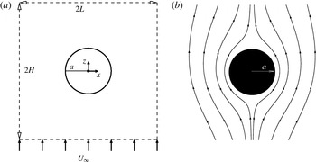
in the far field. The latter scenario is the geometry investigated here (figure 1
a), along with typical streamlines around the cylinder (figure 1
b). The parameters
 $H$
and
 $L$
, respectively, are the vertical and horizontal fluid domain extents where the undisturbed far-field velocity
 $U_{\infty }$
is imposed. We define two characteristic independent aspect ratios
 $\unicode[STIX]{x1D6FC}_{H}=H/a$
and
 $\unicode[STIX]{x1D6FC}_{L}=L/a$
. It should be mentioned that the three-dimensional end effects of the cylinder are not considered in the present study.
Schematic illustration of the geometrical configuration (a) and typical streamlines past a circular cylinder for
 $Re=0.5$
(b).

2.2 The governing equations
The steady-state equations governing the flow are the conservation of mass and momentum (Landau & Lifshitz Reference Landau and Lifshitz1993). By introducing non-dimensional variables
 $\bar{\boldsymbol{u}}=\boldsymbol{u}/U_{\infty }$
,
 $\bar{p}=ap/\unicode[STIX]{x1D707}U_{\infty }$
and
 $\bar{\unicode[STIX]{x1D735}}=a\unicode[STIX]{x1D735}$
, one arrives at the corresponding non-dimensional flow equation given by (bars dropped)
 $$\begin{eqnarray}\displaystyle & \unicode[STIX]{x1D735}\boldsymbol{\cdot }\boldsymbol{u}=0, & \displaystyle\end{eqnarray}$$
 $$\begin{eqnarray}\displaystyle & Re(\boldsymbol{u}\boldsymbol{\cdot }\unicode[STIX]{x1D735})\boldsymbol{u}=-\unicode[STIX]{x1D735}p+\unicode[STIX]{x1D6FB}^{2}\boldsymbol{u}, & \displaystyle\end{eqnarray}$$
with
 $\boldsymbol{u}$
,
 $p$
and
 $\unicode[STIX]{x1D707}$
the fluid velocity, fluid pressure and dynamic viscosity, respectively.
The corresponding boundary conditions are (i) the no-slip condition at the cylinder surface at rest and (ii) the constant vertical velocity
 $U_{\infty }$
in the far field.
2.3 Lattice–Boltzmann method
The velocity and the pressure fields have been computed using an efficient lattice–Boltzmann method (LBM), which has been proved to be a promising method in simulating fluid flow. It has several advantages, including its simple structure, its simplicity in coding, its suitability for modelling multiphase flows and multicomponent fluids as well as its efficiency for parallel computing (Chen & Doolen Reference Chen and Doolen1998; Succi Reference Succi2001). Using the grid refinement technique (Filippova & Hänel Reference Filippova and Hänel1998; Rheinländer Reference Rheinländer2005; Tölke, Freudiger & Krafczyk Reference Tölke, Freudiger and Krafczyk2006), the second-order boundary conditions at the far field (Bönisch, Heuveline & Wittwer Reference Bönisch, Heuveline and Wittwer2005; Liu & Khalili Reference Liu and Khalili2008) and the preconditioning method (Liu & Khalili Reference Liu and Khalili2009), the low convergence rate of standard LBM in reaching the steady-state solution has been overcome.
Frequently, the nine-velocity D2Q9 Bhatnagar–Gross–Krook (BGK) model is used for two-dimensional calculations, leading to flow equations given by Qian, D’Humières & Lallemand (Reference Qian, D’Humières and Lallemand1992) and Qian & Orszag (Reference Qian and Orszag1993),
 $$\begin{eqnarray}f_{i}(\boldsymbol{x}+\boldsymbol{e}_{i}\unicode[STIX]{x1D6FF}_{t},t+\unicode[STIX]{x1D6FF}_{t})-f_{i}(\boldsymbol{x},t)=-\frac{1}{\unicode[STIX]{x1D70F}}[f_{i}(\boldsymbol{x},t)-f_{i}^{(eq)}(\boldsymbol{x},t)],\end{eqnarray}$$
where
 $f_{i}(\boldsymbol{x},t)$
is the single-particle distribution function at position
 $\boldsymbol{x}$
and time
 $t$
along the direction represented by the subscript
 $i$
. Furthermore,
 $\unicode[STIX]{x1D6FF}_{t}$
is the time increment,
 $\unicode[STIX]{x1D70F}$
is the non-dimensional relaxation time connected to the kinematic viscosity via
 $\unicode[STIX]{x1D708}=1/3(\unicode[STIX]{x1D70F}-1/2)\unicode[STIX]{x1D6FF}_{t}$
with
 $c_{s}$
as the speed of sound (set as
 $c_{s}^{2}=1/3$
) and
 $f_{i}^{(eq)}$
is the equilibrium distribution function defined by
 $$\begin{eqnarray}f_{i}^{(eq)}=\unicode[STIX]{x1D714}_{i}\unicode[STIX]{x1D70C}\left[1+\frac{\boldsymbol{e}\boldsymbol{\cdot }\boldsymbol{u}}{c_{s}^{2}}+\frac{\boldsymbol{u}\boldsymbol{u}\boldsymbol{ : }(\boldsymbol{e}_{i}\boldsymbol{e}_{i}-c_{s}^{2}\unicode[STIX]{x1D644})}{2c_{s}^{2}}\right],\end{eqnarray}$$
in which
 $\unicode[STIX]{x1D714}_{i}$
is the weighting factor and
 $\unicode[STIX]{x1D644}$
is the unit tensor. In the D2Q9 model, the discrete velocities are given by
 $\boldsymbol{e}_{0}=0$
and
 $\boldsymbol{e}_{i}=\unicode[STIX]{x1D706}_{i}(\cos \unicode[STIX]{x1D703}_{i},\sin \unicode[STIX]{x1D703}_{i})c$
, with
 $\unicode[STIX]{x1D706}_{i}=1$
,
 $\unicode[STIX]{x1D703}_{i}=(i-1)\unicode[STIX]{x03C0}/2$
for
 $i=1{-}4$
, and
 $\unicode[STIX]{x1D706}_{i}=\sqrt{2}$
,
 $\unicode[STIX]{x1D703}_{i}=(i-5)\unicode[STIX]{x03C0}/2+\unicode[STIX]{x03C0}/4$
for
 $i=5{-}8$
. Here,
 $c=\unicode[STIX]{x1D6FF}_{x}/\unicode[STIX]{x1D6FF}_{t}$
where
 $\unicode[STIX]{x1D6FF}_{x}$
is the lattice spacing. The weighting factors are given by
 $\unicode[STIX]{x1D714}_{0}=4/9$
,
 $\unicode[STIX]{x1D714}_{i}=1/9$
for
 $i=1{-}4$
and
 $\unicode[STIX]{x1D714}_{i}=1/36$
for
 $i=5{-}8$
.
Accordingly, the fluid density and velocity are given respectively by
 $$\begin{eqnarray}\displaystyle & \displaystyle \unicode[STIX]{x1D70C}=\mathop{\sum }_{i}f_{i}, & \displaystyle\end{eqnarray}$$
 $$\begin{eqnarray}\displaystyle & \displaystyle \unicode[STIX]{x1D70C}\boldsymbol{u}=\mathop{\sum }_{i}\boldsymbol{e}_{i}\,f_{i}. & \displaystyle\end{eqnarray}$$
Using the Chapman–Enskog procedure of Chopard & Droz (Reference Chopard and Droz1998), the following mass and momentum equations can be derived from (2.3):
 $$\begin{eqnarray}\displaystyle & \displaystyle \frac{\textstyle \unicode[STIX]{x2202}\unicode[STIX]{x1D70C}}{\textstyle \unicode[STIX]{x2202}t}+\unicode[STIX]{x1D735}\boldsymbol{\cdot }(\unicode[STIX]{x1D70C}\boldsymbol{u})=0, & \displaystyle\end{eqnarray}$$
 $$\begin{eqnarray}\displaystyle & \displaystyle \frac{\textstyle \unicode[STIX]{x2202}(\unicode[STIX]{x1D70C}\boldsymbol{u})}{\textstyle \unicode[STIX]{x2202}t}+\unicode[STIX]{x1D735}\boldsymbol{\cdot }(\unicode[STIX]{x1D70C}\boldsymbol{u}\boldsymbol{u}+p\unicode[STIX]{x1D644}-\unicode[STIX]{x1D748})=0, & \displaystyle\end{eqnarray}$$
where
 $p=c_{s}^{2}\unicode[STIX]{x1D70C}$
is the fluid pressure and
 $\unicode[STIX]{x1D748}$
stands for the deviatoric stresses in the fluid. In the incompressible limit, (2.7) and (2.8) reduce to the incompressible Navier–Stokes equations.
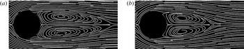
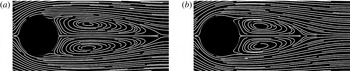
Our LBM model has already been shown to correctly solve the incompressible Navier–Stokes equations (Liu & Khalili Reference Liu and Khalili2008, Reference Liu and Khalili2009). A further verification of the LBM results has been made using the experimental visualization of flow past a circular cylinder (Taneda Reference Taneda1956). For the sake of comparison, here, flow fields with
 $Re=28.4$
and 41.40 are shown in figure 2. The simulated pattern and position of twin vortices at the rear of the cylinder can clearly verify the model.
Flow past a stagnant circular cylinder at
 $Re=28.4$
(a) and
 $Re=41.0$
(b). Note that the simulation boxes were cut so that a direct visual comparison with the results of Taneda (Reference Taneda1956) can be made.
3 Results and discussion
3.1 Discretization error from a no-slip boundary condition at the cylinder surface
The cross-section of the circular cylinder was placed in the centre of the computational domain. Here we seek the optimal number of lattice nodes to adequately discretize the circular cross-section of the cylinder. For this purpose, we examined the drag coefficient
 $C_{D}=F_{D}/(0.5\unicode[STIX]{x1D70C}U_{\infty }^{2}a)$
, with
 $F_{D}$
being the drag force exerted on the cylinder (Veysey & Goldenfeld Reference Veysey and Goldenfeld2007). The drag force
 $F_{D}$
can be determined by integrating the stress tensor over the entire circular cross-section (Landau & Lifshitz Reference Landau and Lifshitz1993). The discretization error for the drag force is expressed by the values given to the cylinder radius
 $a$
. For values of
 $a=20$
,
 $40$
,
 $80$
and
 $160$
, different domain sizes of
 $65\times 65$
,
 $129\times 129$
,
 $257\times 257$
and
 $513\times 513$
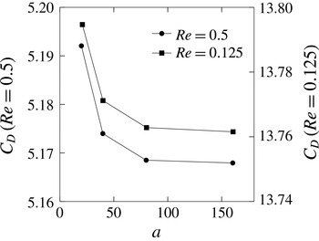
were generated. Figure 3 shows the drag coefficient as a function of cylinder radius for two different Reynolds numbers of
 $Re=0.5$
and 0.125. The drag coefficients display an asymptotic behaviour with an increase of
 $a$
. As depicted in figure 3, increasing
 $a$
from 80 to 160 results in the corresponding relative difference of the drag coefficient (
 $|C_{D}^{160}-C_{D}^{80}|/C_{D}^{160}$
) changing to
 $1.2\times 10^{-4}$
for
 $Re=0.5$
and to
 $8.8\times 10^{-5}$
for
 $Re=0.125$
. Therefore, using the domain size
 $513\times 513$
and
 $a=160$
proved to be sufficient for these calculations.
Drag coefficient as a function of cylinder radius
 $a$
for two different Reynolds numbers.

3.2 Implementation of
 $U_{\infty }$
in the far field

To implement the velocity
 $U_{\infty }$
in the far field, we used the method introduced by Bönisch, Heuveline & Wittwer (Reference Bönisch, Heuveline and Wittwer2008). For numerical simulations, the domain is truncated to a finite subdomain and the so-called ‘artificial boundary conditions’ are imposed at the boundary of the subdomain to replace the conditions in the far field.
The method combines results from dynamical systems theory with matched asymptotic expansion techniques based on the ideas of Goldstein (Reference Goldstein1957) and van Dyke (Reference van Dyke1975) and constructs a smooth divergence-free vector field to represent the far-field velocity. The vector field describes the solution asymptotically at large distances from the body and depends explicitly on the drag and lift. The asymptotic expansion (of order
 $N$
) for the velocity
 $\boldsymbol{u}$
is given by
 $$\begin{eqnarray}\boldsymbol{u}_{N}(x,y)=(U_{\infty },0)+\mathop{\sum }_{n=1}^{N}\mathop{\sum }_{m=1}^{n}\boldsymbol{u}_{n,m}(x,y).\end{eqnarray}$$
The details of the method, including the explicit form of
 $\boldsymbol{u}_{n,m}(x,y)$
, are given by Bönisch et al. (Reference Bönisch, Heuveline and Wittwer2005, Reference Bönisch, Heuveline and Wittwer2008). In our simulation we used (3.1) up to the second-order term
 $(N=2)$
and found that the relative error is reduced by at least two orders of magnitude for a given large aspect ratio when compared with the zeroth-order (
 $N=0$
) results (the results are not shown). The relative error is defined as
 $|C_{D}-C_{D}^{\ast }|/C_{D}^{\ast }$
, where the reference drag coefficient
 $C_{D}^{\ast }$
is obtained from the solution of the steady Navier–Stokes equation using a sufficiently large aspect ratio beyond which the variation of the drag coefficient is negligible. In addition, Liu & Khalili (Reference Liu and Khalili2008) demonstrated that, compared with the zeroth- and first-order terms, inclusion of the second-order term substantially reduced the computational cost for determining the drag at a given precision.
3.3 Illustration of Stokes’ paradox
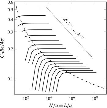
To elucidate Stokes’ paradox graphically, we have employed the Stokes equation and calculated the cylinder drag force as a function of aspect ratio for the range
 $10<H/a=L/a<10^{9}$
. The corresponding normalized drag coefficient as a function of aspect ratio is depicted by the dashed curve in figure 4. Note that, for all Reynolds numbers considered, all the curves collapse onto a single one. The trend shows that, even for the large aspect ratio of
 $10^{9}$
, the normalized drag coefficient has not reached a constant value, indicating that a unique constant solution does not exist for the drag coefficient when the Stokes equation is employed. By comparison, the same calculation has been made by solving the Navier–Stokes equations. In contrast to the former case, the latter shows the existence of a clear constant solution for each Reynolds number when the aspect ratio is sufficiently large. Hence, it is obvious that the addition of an inertial term to the Stokes equation is capable of yielding a unique constant value for the normalized cylinder drag. The solid lines in figure 4 also reveal a further interesting trend. Although the normalized drag coefficients obtained from the Navier–Stokes equation reduce slightly upon decrease of
 $Re$
, they do not collapse onto each other even when
 $Re$
was set to a value of
 $3\times 10^{-5}$
and lower. However, when we replace the cylinder by a sphere, the opposite is the case: i.e. the normalized drag coefficient obtained from the solution of Navier–Stokes equation coincide with the constant Stokes drag of
 $C_{D}=6\unicode[STIX]{x03C0}/Re$
for a sufficiently large aspect ratio and low Reynolds number (not shown).
The normalized drag coefficient as a function of aspect ratio for different Reynolds numbers. Navier–Stokes equation, solid lines; Stokes equation, dashed curve (all curves for different Reynolds numbers collapse onto a single curve). The solid lines belong to cases with decreasing
 $Re$
from
 $2^{0}$
to
 $2^{-15}$
(
 $3\times 10^{-5}$
) in the direction denoted by the arrow.

3.4 Effect of aspect ratio on the flow field
With an adequate implementation of the no-slip and far-field boundary conditions, as explained above, the velocity and pressure fields can be calculated. A typical streamline pattern for
 $Re=0.5$
has been shown in figure 1. The important characteristic of very low-Reynolds-number flows past an infinite circular cylinder is that the presence of the cylinder has an effect on the flow and pressure field over large distances. Even many diameters away to one side, the velocity is appreciably different from the constant far-field velocity
 $U_{\infty }$
(Tritton Reference Tritton1959). Hence, the correct calculation of the near-object primary hydrodynamic quantities (velocity, pressure) depends significantly on the distances from the object where the far-field boundary conditions are imposed.
To highlight the differences in the near-cylinder velocity field arising from different
 $\unicode[STIX]{x1D6FC}_{L,H}$
, we computed the velocity field and plotted the boundary of those regions around the cylinder within which the vertical velocity components grow from zero to 90 %, 95 % or 99 % of the constant undisturbed
 $U_{\infty }$
, referred to in the following as the near-cylinder layer. Here we calculate the upstream (
 $\unicode[STIX]{x1D6FF}_{up}$
) and transverse (
 $\unicode[STIX]{x1D6FF}_{tr}$
) near-cylinder layers. The latter is the layer thickness left or right of the cylinder.
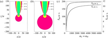
In the example shown in figure 5(a,b), the layer thicknesses have been calculated at
 $Re=0.5$
for two different aspect ratios of
 $\unicode[STIX]{x1D6FC}_{H,L}=200$
and 6500. Although an aspect ratio of 200 might seem sufficient, this aspect ratio (figure 5
a) artificially squeezes the near-cylinder layer compared to the case with an aspect ratio of 6500 (figure 5
b). Despite the fact that low-
 $Re$
flows are considered to be those with
 $Re\leqslant 0.1$
, figure 5 demonstrates that the ratio of domain size to diameter plays a significant role, even for
 $Re=0.5$
. This demonstrates the drastic impact of the aspect ratio on the velocity and pressure fields. Hence, the effect of
 $\unicode[STIX]{x1D6FC}_{L,H}$
has to be examined with care if one is to mimic adequately low-Reynolds-number flows past objects placed in effectively infinite domains.
Effect of aspect ratio (
 $\unicode[STIX]{x1D6FC}_{H,L}$
) on the thickness of the near-cylinder region within which the vertical velocity component has reached 90 %, 95 % and 99 % of
 $U_{\infty }$
for
 $Re=0.5$
: (a)
 $\unicode[STIX]{x1D6FC}_{H,L}=200$
and (b)
 $\unicode[STIX]{x1D6FC}_{H,L}=6500$
. The tiny black circle in the centre of both panels represents the cylinder cross-section. (c) The upstream near-cylinder layer thickness (
 $\unicode[STIX]{x1D6FF}_{up,99\,\%}$
) and the transverse one (
 $\unicode[STIX]{x1D6FF}_{tr,99\,\%}$
) as a function of aspect ratio. The
 $\unicode[STIX]{x1D6FF}_{up,99\,\%}$
and
 $\unicode[STIX]{x1D6FF}_{tr,99\,\%}$
values were non-dimensionalized by the cylinder radius
 $a$
.

The shrinkage of the flow field affects both the upstream and transverse near-cylinder layer when the aspect ratios are too small (see figure 5
c). The extensive flow simulations covering a wide range of
 $\unicode[STIX]{x1D6FC}_{H}$
and
 $\unicode[STIX]{x1D6FC}_{L}$
shown in figure 5(c) indicate that a sufficiently large threshold value of the ratio of domain extent to cylinder radius (
 $\unicode[STIX]{x1D6FC}_{L,H}$
) must be considered in order to mimic correctly the velocity and pressure fields. As can be seen from the trend (figure 5
c), both
 $\unicode[STIX]{x1D6FF}_{up,99\,\%}$
and
 $\unicode[STIX]{x1D6FF}_{tr,99\,\%}$
still increase. Thus, the aspect-ratio range considered still does not mirror the unboundedness of the flow domain. As illustrated by the auxiliary vertical dashed line in figure 5(c),
 $\unicode[STIX]{x1D6FC}_{H,L}\leqslant 200$
, for example, leads to
 $\unicode[STIX]{x1D6FF}_{up,99\,\%}=150$
compared to the larger
 $\unicode[STIX]{x1D6FF}_{up,99\,\%}\approx 200$
for the larger aspect ratio of 6500. Similarly, the thickness of
 $\unicode[STIX]{x1D6FF}_{tr,99\,\%}$
changes from
 ${\approx}$
5 to
 ${\approx}$
11 if a larger, more realistic domain extent is chosen. Hence, the calculation of any secondary hydrodynamic quantity, such as drag, will suffer from non-physical deficiencies of mapping an infinite domain into one that is too small. To identify the minimum necessary value of
 $\unicode[STIX]{x1D6FC}_{L,H}$
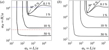
for an accurate calculation of the velocity field and the drag coefficient, we performed a systematic sensitivity analysis of the flow field and drag coefficient as a function of the Reynolds number. For ease of comparison, only the drag coefficient data have been shown. The variation of drag coefficient as a function of a large range of
 $\unicode[STIX]{x1D6FC}_{L}$
for two distinct Reynolds numbers of
 $Re=0.06$
and 0.008 is shown in figure 6. Starting from the reference solution, shown as the 0 % error curve, one can observe different behaviours depending on the values of
 $\unicode[STIX]{x1D6FC}_{L}$
and
 $\unicode[STIX]{x1D6FC}_{H}$
. Obviously any combination of
 $\unicode[STIX]{x1D6FC}_{H}$
and
 $\unicode[STIX]{x1D6FC}_{L}$
on the 0 % error curve or in its vicinity lead to optimal results. However, any large value of
 $\unicode[STIX]{x1D6FC}_{L}$
will lead to erroneous results if
 $\unicode[STIX]{x1D6FC}_{H}$
is small (see the horizontal red dot-dashed line in figure 6
a). For some values of
 $\unicode[STIX]{x1D6FC}_{H}$
, the 0 % error curve can be crossed twice (see the horizontal blue dashed line in figure 6
a), meaning that both
 $\unicode[STIX]{x1D6FC}_{L}$
values would provide optimal results. In short, the most optimal solutions can be obtained for the combination of
 $\unicode[STIX]{x1D6FC}_{L}$
and
 $\unicode[STIX]{x1D6FC}_{H}$
that lies on the minimum of the 0 % error curve. The minimum of this curve
 $M^{\ast }$
corresponds to the smallest necessary aspect ratio, ensuring a constant vertical velocity in the far field. Figure 6 also shows curves along which the relative drag errors were for 1 %, 10 % and 50 %.
Sensitivity analysis of the drag coefficient as a function of
 $Re$
. The error percentages given refer to the relative error of the drag coefficient,
 $|C_{D}-C_{D}^{\ast }|/C_{D}^{\ast }$
, with respect to
 $C_{D}^{\ast }$
as the reference drag for
 $Re=0.06$
(a) and
 $Re=0.008$
(b).

Comparison of the two panels in figure 6 reveals that the smaller the Reynolds number becomes, the larger the aspect ratios will be in low-Reynolds-number flows past objects placed in effectively infinite domains. For example, in the case of
 $Re=0.06$
the minimum can be obtained already with
 $\unicode[STIX]{x1D6FC}_{L}\approx 400$
and
 $\unicode[STIX]{x1D6FC}_{H}\approx 3000$
, while for the smaller Reynolds number of
 $Re=0.008$
much bigger aspect ratios (
 $\unicode[STIX]{x1D6FC}_{L}\approx 3300$
and
 $\unicode[STIX]{x1D6FC}_{H}\approx 23\,400$
) are required.
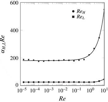
The optimal aspect ratio combinations, i.e. the coordinates of
 $M^{\ast }$
, were calculated for a wide range of
 $Re<1$
. The resulting trend is depicted in figure 7. A close inspection of the trends suggests functional relationships of the form
 $$\begin{eqnarray}\displaystyle & \displaystyle \unicode[STIX]{x1D6FC}_{L}\approx \frac{27}{Re}, & \displaystyle\end{eqnarray}$$
 $$\begin{eqnarray}\displaystyle & \displaystyle \unicode[STIX]{x1D6FC}_{H}\approx \frac{182}{Re} & \displaystyle\end{eqnarray}$$
between the Reynolds number and aspect ratios. In addition, considering the definition of
 $\unicode[STIX]{x1D6FC}_{H}$
and
 $\unicode[STIX]{x1D6FC}_{L}$
, one can obtain the minimum necessary horizontal and vertical domain extents for mimicking infinite domains. In very slow flows, these minima increase with the inverse of the Reynolds number.
Domain size effect as a function of
 $Re$
for very slow flows. The circles and squares represent computed results while solid lines are their best fits.

3.5 An improved relation for the drag coefficient
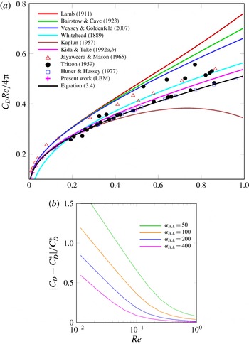
We calculated the normalized drag coefficients as a function of
 $Re$
(figure 8
a). Some classical experimental and analytical results have also been plotted. The experimental studies can be divided into two categories. In the first category, the flow was passing around a very thin hanging wire, ahead of which a mesh screen was placed to generate a uniform velocity profile (e.g. Finn Reference Finn1953; Tritton Reference Tritton1959). The distance between the wire and mesh screen, which corresponds to
 $\unicode[STIX]{x1D6FC}_{H}$
defined above, can indeed impose artificial bounds on the flow field. As an example, we revisited the drag coefficient measurement of Finn (Reference Finn1953). Compared with our calculations for
 $Re=0.03$
and
 $\unicode[STIX]{x1D6FC}_{H}\approx 1000$
, the relative error of his measurement amounts to around 10 %. In the second category, a long solid cylinder with a finite small diameter was sinking normal to its axis in a container filled with fluid (e.g. Jayaweera & Mason Reference Jayaweera and Mason1965; Huner & Hussey Reference Huner and Hussey1977). Here
 $\unicode[STIX]{x1D6FC}_{L}$
is the critical parameter. In the experiment of Jayaweera & Mason (Reference Jayaweera and Mason1965), for example, the relative error of the drag coefficient was around 20 %, based on our calculations for
 $Re=0.009$
and
 $\unicode[STIX]{x1D6FC}_{L}\approx 700$
. Among all existing experiments, the data obtained by Huner & Hussey (Reference Huner and Hussey1977) can be considered as the best for at least two reasons: first, they contain less scatter; and second, they are corrected by themselves empirically to mimic the infiniteness of cylinder length and aspect ratio. When we decreased the aspect ratio gradually, our numerical data first approached the experimental results of Tritton (Reference Tritton1959) and then those of Jayaweera & Mason (Reference Jayaweera and Mason1965). The negative effect of too small aspect ratios on the drag coefficient has been demonstrated in figure 8(b). The relative errors of smaller domain sizes compared to the reference values grow drastically with decrease in
 $Re$
. For example, at
 $Re=0.01$
and
 $L/a=400$
, the drag value still contains 21 % deviation from its correct reference value. The same ratio of domain size to cylinder radius (
 $L/a$
) even led to 50 % deviation when
 $Re$
was reduced to
 $Re=0.002$
.
(a) Comparison of the normalized drag coefficients obtained in previous experiments (symbols) and analytical approximations (solid lines) versus accurate numerical data obtained in the present study (pink plus symbols). (b) Response of the relative error of the drag coefficient to small aspect ratios as a function of
 $Re$
.

Based on an integral approach of asymptotic expansions for low-Reynolds-number flow past an arbitrary cylinder, Kida & Take (Reference Kida and Take1992a
,Reference Kida and Take
b
) provided a relation for the drag coefficient as a function of
 $Re$
as
 $C_{D}=(4\unicode[STIX]{x03C0}\unicode[STIX]{x1D6FF}/Re)[2/(1+\sqrt{1+3.5\unicode[STIX]{x1D6FF}^{2}})]$
. Here,
 $\unicode[STIX]{x1D6FF}=[0.5-\unicode[STIX]{x1D6FE}-\log (Re/4)]^{-1}$
with
 $\unicode[STIX]{x1D6FE}=0.577216\ldots$
as Euler’s constant. However, due attention has not been paid to this relation. Among all available approximate solutions, these results produced the closest fit to our numerical results. Furthermore, both our numerical results and the solution of Kida & Take (Reference Kida and Take1992a
) matched best with the experimental results of Huner & Hussey (Reference Huner and Hussey1977).
Using our careful numerical data (figure 8), we found that the most suitable solution is provided when replacing the factor 3.5 in the relation of Kida & Take (Reference Kida and Take1992a ) by 4.3, arriving at
 $$\begin{eqnarray}\displaystyle C_{D}=\frac{4\unicode[STIX]{x03C0}\unicode[STIX]{x1D6FF}}{Re}\left(\frac{2}{1+\sqrt{1+4.3\unicode[STIX]{x1D6FF}^{2}}}\right). & & \displaystyle\end{eqnarray}$$
This relation is valid for very low Reynolds numbers and has been tested in this study for the range of
 $3\times 10^{-5}\leqslant Re\leqslant 1$
.
4 Application of drag relation for marine microbiological studies
The significance of minimum aspect ratios in very low-
 $Re$
flows becomes evident in the context of slowly sinking marine micro-organisms, such as cylindrical diatoms, filamentous green algae and desmids, and carbon-containing particles, which export carbon from the upper ocean towards the ocean floor. An important issue is the estimation of nutrient uptake by sinking particles, described by the Sherwood number (
 $Sh$
, the ratio between the total flux of a nutrient solute arriving at the surface of a moving cell and the purely diffusive flux of a stationary cell, equivalent to the enhancement of nutrient uptake (Karp-Boss & Jumars Reference Karp-Boss and Jumars1996)) as a function of Péclet number (
 $Pe=Ua/D$
), the effectiveness of advective transport compared with diffusive transport (Karp-Boss & Jumars Reference Karp-Boss and Jumars1996). The empirical relation for Sherwood number was given by Munk & Riley (Reference Munk and Riley1952) as
 $$\begin{eqnarray}\displaystyle Sh=0.8(2Pe)^{0.31}. & & \displaystyle\end{eqnarray}$$
For a given excess density (
 $\unicode[STIX]{x0394}\unicode[STIX]{x1D70C}=(\unicode[STIX]{x1D70C}_{p}-\unicode[STIX]{x1D70C})/\unicode[STIX]{x1D70C}$
, with
 $\unicode[STIX]{x1D70C}_{p}$
and
 $\unicode[STIX]{x1D70C}$
the particle and fluid density, respectively) and particle size (with radius
 $a$
), one can arrive at the particle’s terminal velocity
 $U$
, from which
 $Pe$
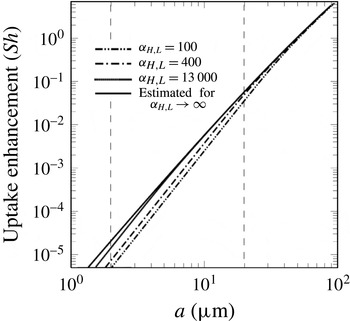
can be determined. Using (4.1), nutrient uptake enhancement can be calculated as a function of particle size (figure 9) for
 $\unicode[STIX]{x0394}\unicode[STIX]{x1D70C}=0.1$
, a value typical for these micro-organisms. For the cylindrical diatom Leptocylindrus minimus, with typical radius
 $a\approx 2~\unicode[STIX]{x03BC}\text{m}$
,
 $Sh$
obtained from a small aspect ratio (100) is underestimated five times compared to the larger aspect ratio of 6500 (line for 6500 not shown). Similarly, a 200 % error in the amount of calculated uptake enhancement will be made for Guinardia flaccida with a typical radius
 $a\approx 20~\unicode[STIX]{x03BC}\text{m}$
when an insufficient aspect ratio of 100 is used.
Effect of aspect ratios on the uptake enhancement (
 $Sh$
) for a typical excess density of
 $\unicode[STIX]{x0394}\unicode[STIX]{x1D70C}=0.1$
. The solid black line represents the present work.

5 Conclusion
We revisited the problem of the steady flow of an unbounded viscous fluid past an infinitely long stationary circular cylinder. We computed the drag coefficient as a function of increasing ambient fluid extents for
 $3\times 10^{-5}<Re<1$
and illustrated Stokes’ paradox graphically. Our computations reveal the existence of minimum aspect ratios necessary to best mimic very low-Reynolds-number flows of cylindrical particles in effectively infinite domains. In addition, we suggest an improved relation for the drag coefficient as a function of Reynolds number. Our results are useful for understanding the impact of inevitable domain sizes when objects move in unbounded fluids. The values given for vertical and horizontal aspect ratios (
 $\unicode[STIX]{x1D6FC}_{H}$
,
 $\unicode[STIX]{x1D6FC}_{L}$
) serve directly as a guideline for the ratios of container size to the object radius in experiments and computations. Beyond technical applications, this relation can be used to address important questions in the field of marine microbiology in studies concerning the activities of many cylindrical marine micro-organisms and plants.
Acknowledgements
This work was supported by the Max Planck Society (MPG). The authors would like to thank N. Moradi, N. Goldenfeld and P. Jumars for their valuable discussions and S. Ahmerkamp for reproduction of the figures. B. L. would like to thank the Leibniz Institute for Baltic Sea Research (IOW) for its financial support.